1. Introduction
The emerging global constellation of the third generation of geostationary satellites carry advanced instruments with spectral, spatial, and radiometric resolutions comparable to flagship satellite sensors such as MODIS and VIIRS [
1]. More importantly, the new geostationary sensors continuously scan Earth’s full disk every ~10 min, generating data streams of much higher temporal resolution than the Low Earth Orbit (LEO) satellites [
2,
3,
4,
5]. Such datasets provide valuable and unique opportunities for Earth monitoring [
6,
7].
Geostationary NASA Earth Exchange (GeoNEX) is a collaborative effort led by NASA, NOAA, and many other research institutes to explore the potential of geostationary data streams in generating rigorous and systematic science products. We introduced the GeoNEX Level 1G products, including the top-of-atmosphere (TOA) reflectance and brightness temperature, in a previous paper [
8]. The GeoNEX Level 1G products include radiometrically calibrated and geometrically rectified TOA BRF and brightness temperatures reprojected onto a common grid in the geographic projection [
8,
9,
10]. The common grid covers Earth’s surface from 60° N to 60° S and is divided into 6° × 6° tiles that were numbered from 0 to 59 horizontally and from 0 to 19 vertically. The spatial resolutions of the grid are 0.005°, 0.01°, and 0.02° in correspondence to the native 0.5 km, 1 km, and 2 km (nadir) spatial resolution of the original geostationary data in the fixed-point projection. The temporal resolution of the products is also the same as the original data, being 10–15 min for full-disk scans. The L1G data include accurate sun-target-satellite geometry information, in particular the solar zenith and azimuth angles, for each pixel in the domain at every time step. The data are archived in the EOS-HDF format and publicly accessible at the GeoNEX data portal (
https://data.nas.nasa.gov/geonex; data were last accessed on 4 February 2022). More details regarding the GeoNEX L1G products can be found in [
8].
The next (Level 2) step in the GeoNEX processing chain is atmospheric correction, which removes the effects of atmospheric absorption and scattering from the L1G TOA radiances to retrieve the surface reflectance (SR) and, as a by-product, the corresponding atmospheric aerosol optical depth (AOD). The algorithm we are adapting for this task is the Multiangle Implementation of Atmospheric Correction (MAIAC) system [
11,
12,
13,
14,
15,
16]. In this paper, however, we introduce a new algorithm, which is inspired by MAIAC and developed from its framework, to particularly exploit the diurnal variability in geostationary observations for atmospheric correction. (In this paper we do not distinguish the differences between “diurnal” and “daytime” but may use them interchangeably.) The algorithm, named GeoNEX-AC, is not intended to replace MAIAC as the operational algorithm for the GeoNEX L2G products but rather be a tool for diagnostic analyses. Before we introduce the motivations behind the development of GeoNEX-AC, let us review some of the basic ideas of atmospheric correction.
Because the TOA radiance is a composite of solar radiations reflected by the surface and backscattered by the atmosphere, retrieving SR or/and the AOD from the TOA measurements is fundamentally under-constrained [
17]. Additional information or a simplification must be introduced so that a solution may be obtained. Such information can be derived from various aspects of optical remote sensing data in spatial, spectral, angular, and temporal dimensions. Different algorithms have been developed to exploit different information sources.
For instance, atmospheric aerosol loading generally varies smoothly over spatial scales under 50 km [
18]. Therefore, we may opt to retrieve the AOD over dark pixels, where the measured TOA reflectance is mainly regulated by the atmosphere and thus the retrieved AOD is more accurate [
19]. This is the basic idea underlying the MODIS Dart Target algorithm [
20,
21,
22]. Note that pixels that are bright in some spectral bands could be dark in other bands. For instance, the visually bright deserts indeed appear dark in the 0.41 µm spectral region, which has motivated the development of the Deep Blue algorithm to retrieve the AOD over deserts and similar regions [
23,
24,
25].
A very common approach adopted by existing atmospheric correction algorithms to decouple the atmospheric and the surface regulation on TOA reflectance is based on the notion of spectral dependency between different bands [
19]. On one hand, because the AOD generally decreases with wavelengths following the power law [
26], its regulation to the TOA reflectance in the Short-Wave Infrared (SWIR) range (e.g., 2.2 µm) is relatively small. This allows us to more accurately retrieve the surface reflectance for the SWIR band. On the other hand, it was found that the ratios between the visible (i.e., Blue and Red) and the SWIR bands (e.g., 2.2 µm) over densely vegetated pixels are statistically stable [
19,
20,
22]. When the band ratios are determined a priori, we can easily estimate the reflectance of the visible bands from the SWIR band [
19] and subsequently retrieve the AOD in the visible spectral range [
20,
22].
In general cases (without the restriction on dense vegetation pixels), the spectral band ratios can vary by land surface types as well as the illumination-view geometry [
27,
28]. Different approaches have been developed to determine the spatial and the temporal variations in the spectral band ratios. Since Collection 5, the MODIS Dark Target algorithm has used empirical models to account for land-cover and angular variations in the band ratios [
20]. The latest Visible/Infrared Imager Radiometer Suite (VIIRS) AOD algorithm develops a spatial database of spectral band ratios to account for their spatial variability [
29]. The MAIAC algorithm dynamically maintains band ratios at various illumination-view geometries with the latest surface reflectance retrievals at each pixel [
11,
16].
Another important consideration of atmospheric correction algorithms is how to treat the anisotropy of the surface reflectance. A full description of the angular dependence of surface reflectance (SR) requires the Bi-directional Reflectance Distribution Function (BRDF), which itself is challenging to model. The simplest approach is to neglect the surface anisotropy by assuming the surface to be Lambertian. The Lambertian assumption has the advantage of easy implementation and has been adopted in many atmospheric correction and aerosol retrieval algorithms, such as 6S [
30,
31], Dark Target [
20], ATREM [
32], ISOFIT [
33], and many others [
34,
35]. This approach, however, neglects the angular variations in the surface reflectance, which can be an important information source for atmospheric correction for GEO observations.
Recent atmospheric correction algorithms have emerged that explicitly account for the SR anisotropy. One example is the Aerosol and surface albedo Retrieval Using a directional Slitting method-application to GEOstationary data (AERUS-GEO) algorithm originally developed in [
36,
37] to process observations from the Spinning Enhanced Visible and Infra-Red Imager (SEVIRI) on board the Meteosat Second Generation (MSG) geostationary satellite. The algorithm adopts the semi-analytical Ross-Thick–Li-Sparse (RTLS) model to represent surface BRDF and evaluates its regulation on the TOA reflectance in a linearized semi-physical model at low computational cost [
36]. The AERUS-GEO algorithm has been applied to process GOES ABI and Himawari AHI data [
38].
A more rigorous and comprehensive algorithm that explicitly accounts for the surface BRDF effects is MAIAC. Like AERUS-GEO, MAIAC also adopts the RTLS BRDF model. However, unlike AERUS-GEO, MAIAC rigorously derives the expression of the TOA reflectance (as a function of surface BRDF) with the help of Green’s function method [
39,
40]. Because the RTLS model essentially represents BRDF as a combination of kernel functions (of illumination and view geometries) weighted by a few linear parameters, MAIAC is able to efficiently and accurately exploit the angular dimension of the satellite observations.
MAIAC also exploits temporal information from time series of satellite observations. The algorithm uses the differences in space-time variability between land surface and atmospheric optical conditions (e.g., clouds, aerosols, etc.) to separate land and atmospheric signals. It regularly monitors time series of surface reflectance in the Red, the Near Infrared (NIR), and the SWIR bands to detect potential changes in surface conditions due to weather (e.g., rain/snow) or natural disturbances (e.g., fires). The algorithm “remembers” and dynamically updates a set of physical signatures for each grid cell, including full spectral BRDF, spectral and thermal contrasts, and metrics of spatial variability from higher resolution channels with the latest measurements. These functional requirements increase the complexity of the implementation of the MAIAC algorithm, but help improve its capability in cloud/snow detection, which is a dominant error source in land remote sensing [
11,
12]. The data composition approach described above is based on the assumption that surface properties are stationary at short time scales. The choice of composition time windows is clearly affected by the satellite’s revisit frequency. LEO sensors such as MODIS and VIIRS complete the global coverage at daily scales. By the well-known Nyquist–Shannon sampling theorem [
41], this means that these observations cannot be used to resolve surface processes that occur on bi-diurnal or shorter time scales. This time-scale limit can be much longer due to cloud contamination and issues in practice. For instance, the MAIAC algorithm composites MODIS observations with a sliding window up to 16 days [
16], which is by no means ideal and only reflects the limitation of the LEO data. We will show in this paper that the 10-min data frequency of the GEO sensors provides a most promising alternative to address the issue.
The above brief review shows that MAIAC has many advantages in processing multi-angular satellite data. For this reason, we are adapting it as the operational algorithm to generate GeoNEX Level 2 products. At the same time, because MAIAC is also applied to process data streams from many other satellites, such as MODIS and VIIRS, we are interested in the question: “what advantages do geostationary datasets have, in comparison with their LEO counterparts, that facilitate atmospheric correction?”
This paper is set to answer this question. We will demonstrate that the diurnal variability in the geostationary TOA reflectance (or radiance), as represented by the high-temporal-resolution (i.e., ~10 min) time series, contains unique information that helps us separate the surface and the atmospheric signals without invoking other common techniques such as the spectral band ratios. We develop the GeoNEX-AC algorithm particularly to exploit the temporal and the angular information from the diurnal variations in the geostationary data. We will show that our algorithm has good performance on various, even challenging, land cover types. In addition, we will show that the retrieval results from our algorithm have the potential to help validate and refine conventional atmospheric correction techniques.
2. Materials and Methods
2.1. Data
We use the GeoNEX Level 1G products [
8] of GOES 16 ABI in this study. The products include the bidirectional reflectance factor (BRF) for the reflective bands and brightness temperature (BT) for the emissive bands [
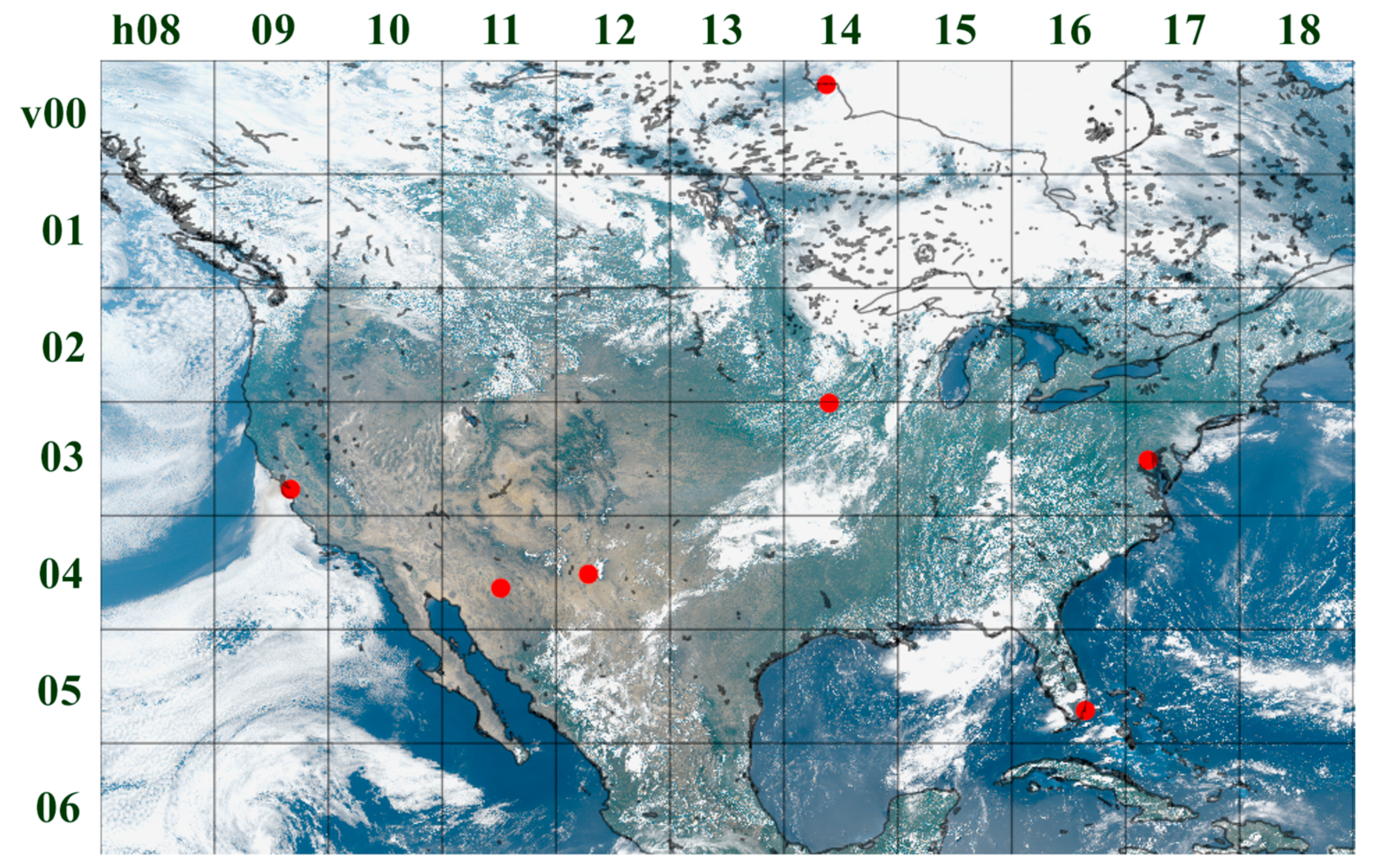
8]. As GOES 16 is parked over the equator at 75.2° W, its GeoNEX spatial domain covers both North and South America from 138° W (Horizontal Tile 7) to 18° W (Horizontal Tile 26) and from 60° N (Vertical Tile 0) to 60° S (Vertical Tile 19).
Figure 1 shows the tiles over the conterminous Unites States (CONUS).
For the interest of this paper, we developed and tested our atmospheric correction algorithm with time series of the GeoNEX L1G products over selected AERONET sites, which are listed in
Table 1 and indicated in
Figure 1. These sites were specifically chosen to cover a diverse range of representative geographic locations or/and surface types. We used the Level 2 Aerosol Optical Depth (AOD) products [
42,
43] measured at the AERONET sites to validate the retrieval results from our algorithm.
2.2. Radiative Transfer Model
Atmospheric radiative transfer models (RTMs) are well-developed tools to simulate the propagation of sunlight, including the absorption and the scattering of photons by air molecules and aerosols, in the atmosphere. The RTMs used in MAIAC include the Spherical HARMonics code (SHARM) [
44] and the Intensity and POLarization code (IPOL) [
45], both of which represent the state of the art [
46]. The SHARM code performs fast and accurate simulations of the monochromatic radiance at the top of the atmosphere over spatially variable surfaces with Lambertian or anisotropic reflectance. It assumes that the atmosphere is laterally uniform and aerosols are mainly contained in the bottom atmosphere layer. The code computes the spectral absorption of six major atmospheric gases (H
2O, CO
2, CH
4, NO
2, CO, and N
2O) based on the HITRAN 2008 database [
47] using a line-by-line interpolation and profile correction method [
48] for the GOES ABI and Himawari AHI spectral response functions. Absorption by Ozone is corrected separately with the six-hourly NCEP Global Data Assimilation System (GDAS) data. MAIAC uses the IPOL code to simulate the effects of polarization on the transport of solar radiation, especially those induced by the scattering of atmospheric particles. The solutions of IPOL are then used to update the atmospheric path reflectance in the SHARM simulation [
16].
A particular advantage of the SHARM model is that it rigorously decouples the atmospheric transport of sunlight from its interactions with the surface via the method of Green’s functions [
39,
40]. This feature allows the model to fully describe the solutions of the TOA reflectance in terms of a few surface BRDF parameters and kernel functions [
16]. The current implementation of MAIAC uses the Ross-thick–Li-sparse (RTLS) BRDF model [
49], which represents the surface BRF (
ρ) as the sum of Lambertian, volume scattering, and geometric optical components:
where
and
are the kernel functions for volume scattering and geometric optical components (the Lambertian kernel is normalized to be 1), respectively, and
are the sets of weights for the corresponding components. Note that the kernel functions are purely determined by the sun-satellite geometry, including the cosines of the solar and the view zenith angles (
and
) and the relative azimuth angle (
), and therefore can be accurately calculated.
With the RTLS parameters, the TOA reflectance is explicitly expressed as
where
represents the atmospheric path reflectance. The functions
,
,
, and
are calculated with a few basic functions representing different hemispheric integrals of downward path radiance, atmospheric Green’s function, and the RTLS kernels [
11]. These functions depend on the illumination-view geometry and aerosol properties.
MAIAC pre-calculates Green’s functions on selected sun-satellite angles and aerosol levels and stores them in Look-Up Tables (LUTs), which enable fast and accurate simulations of TOA reflectance in operational runs. MAIAC uses eight different dynamic aerosol models for various regions of the world [
16]. Particular to this study, MAIAC separately uses two aerosol models for Eastern and Western United States, both of which are calibrated with regional AERONET observations [
43] and represent the state of the art [
16]. MAIAC also generates a separate LUT for a Rayleigh atmosphere, which has no aerosol loading and thus considers only the molecular scattering of the photons. It uses the 1976 US Standard Atmosphere profile in computing the LUTs over the domain of CONUS. We use the same DEM as in the MODIS MAIAC to correct for variations in surface pressures. Details of the latest technical aspects of the MAIAC LUT can be found in [
16].
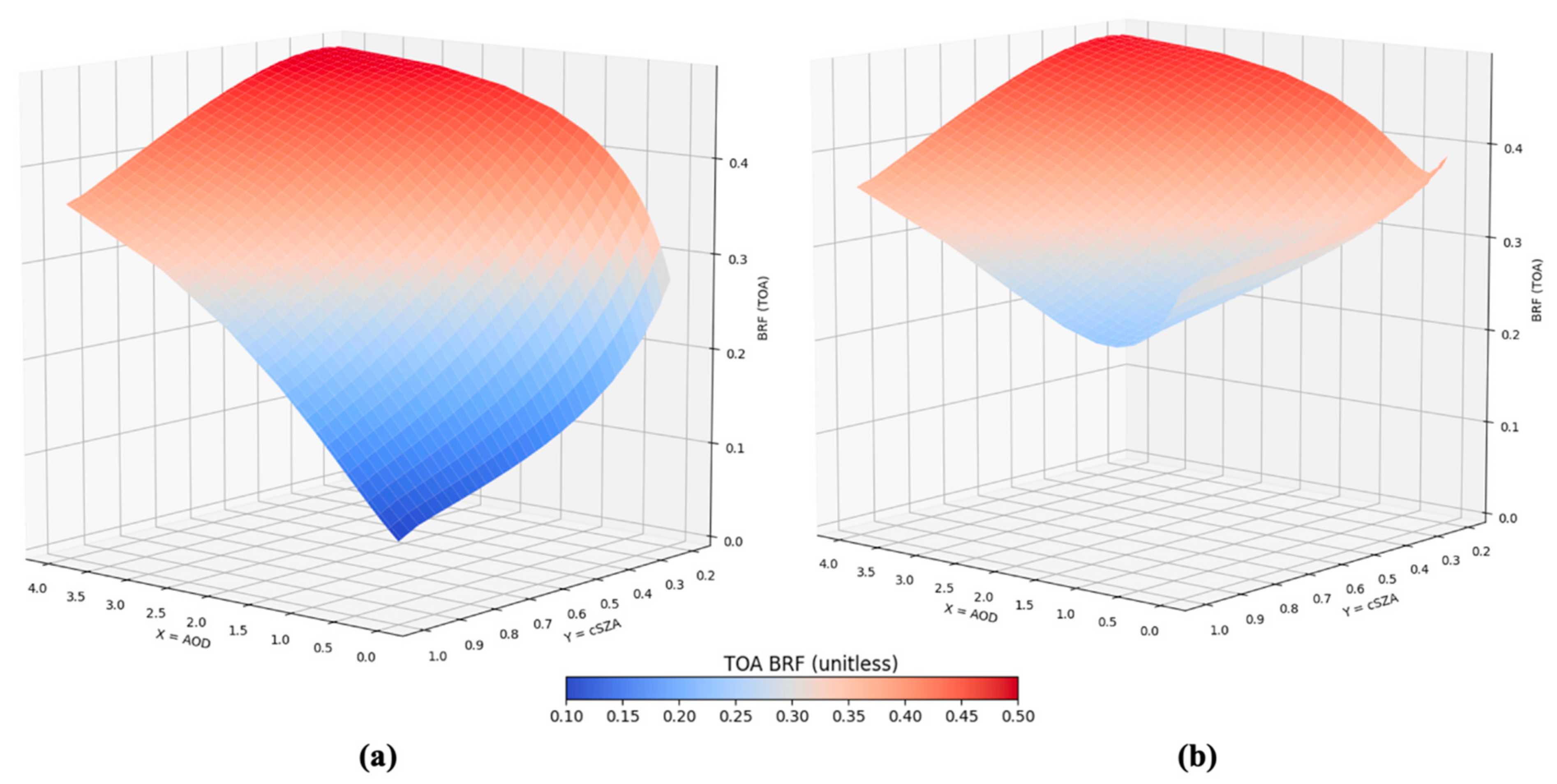
Figure 2 illustrates the use of the MAIAC RTM in simulating the Blue-band (0.47 µm) TOA BRFs at the Tucson site. Because the view angles of geostationary satellites are fixed for a given pixel, we mainly consider the dependence of TOA BRF on solar angles (
and
), aerosol optical depth (AOD), and surface reflectance (
). For the purpose of illustration, we keep the relative azimuth angle constant and simplify the surface to be Lambertian so that it is easy to visualize the simulation results as functions of solar zenith angles (SZA) and AOD levels at the specified surface reflectance. In
Figure 2a, the surface reflectance is zero (“black soil”) and thus the TOA BRF is contributed totally by atmospheric path reflectance. It is clear that the path reflectance increases as the AOD and SZA increase (the cosine of SZA, cSZA, decreases). When the surface reflectance increases to 0.3 (
Figure 2b), the contribution from the surface-reflected component in the TOA signal becomes more important at lower AOD levels (AOD < 0.5). However, its importance decreases at higher AOD levels (AOD > 1) or/and larger SZAs (SZA > 60° or cSZA < 0.5). These results are expected from the well-known fact that solar radiation in the Blue band is prone to atmospheric scattering.
The example shown in
Figure 2 illustrates the forward simulation with the MAIAC RTM. In comparison, atmospheric correction is an inverse problem, where the surface BRDF parameters and the AOD level need to be determined from the observed TOA BRFs. We show below that this is essentially achieved by identifying the optimal combinations of AOD and surface reflectance (and its component) so that the simulated diurnal variations in TOA BRFs best match the observations.
2.3. Algorithm Overview
We give a quick overview of our algorithm (
Figure 3) in this section before discussing the major components in detail in the following sections.
In order to exploit information from the diurnal variability in the TOA observation, our processing starts with reading in the whole diurnal cycles of TOA BRFs, brightness temperatures, and other ancillary data (e.g., climate reanalysis products). The first major step (Box 1) is to distinguish smooth and rough segments of the time series with specifically designed Roughness Indices for the visible bands. Only smooth segments of consecutive data points are deemed suitable for further analysis. The next step (Box 2) conducts initial tests to further filter out observations that are likely contaminated by persistent clouds. This step temporarily labels the rest of the data points as clear observations. The workflow proceeds only if there are at least three clear observations remaining in the diurnal cycle.
For the next stage of processing, we first check if prior surface BRDF parameters exist. If not, the workflow proceeds only when the day is clear and there are sufficient clear-sky data points in the diurnal time series. We perform the clear-day atmospheric correction algorithm to fully retrieve the BRDF parameters and the daily mean AOD, and calculate the corresponding surface reflectance (Box 5). The BRDF information will be saved and serve as the prior information for the next processing cycle.
If the BRDF has been previously retrieved, the prior information is used to refine the (partial) cloud/snow tests (Box 3). It is followed by an initial estimation of surface reflectance and AOD with the partial-clear-day algorithm (Box 4). If the day is fully clear, the BRDF parameters, AOD, and SR will be estimated for the second time with the clear-day algorithm (Box 5).
The final step in the processing chain is to update the posterior BRDF information (Box 6). For clear days, the basic strategy is to use the newly retrieved BRDF parameters as the posterior. This approach is taken as a measure to refresh the “memory” of the processing and therefore remove potential biases accumulated from previous days. For partially clear days, we update the posterior BRDF by compiling the surface reflectance in the past few days (up to 32 cloud-free observations) and re-estimate the RTLS parameters from the composited time series. The processing iterates at daily time steps and generates outputs of 10-min surface reflectance, daily BRDF parameters, and daily mean AOD at the end of every day.
2.4. Diurnal Variability and Smoothness/Roughness Index
We started to develop our atmospheric correction algorithm by examining the characteristics of the diurnal variations in the observed TOA reflectance.
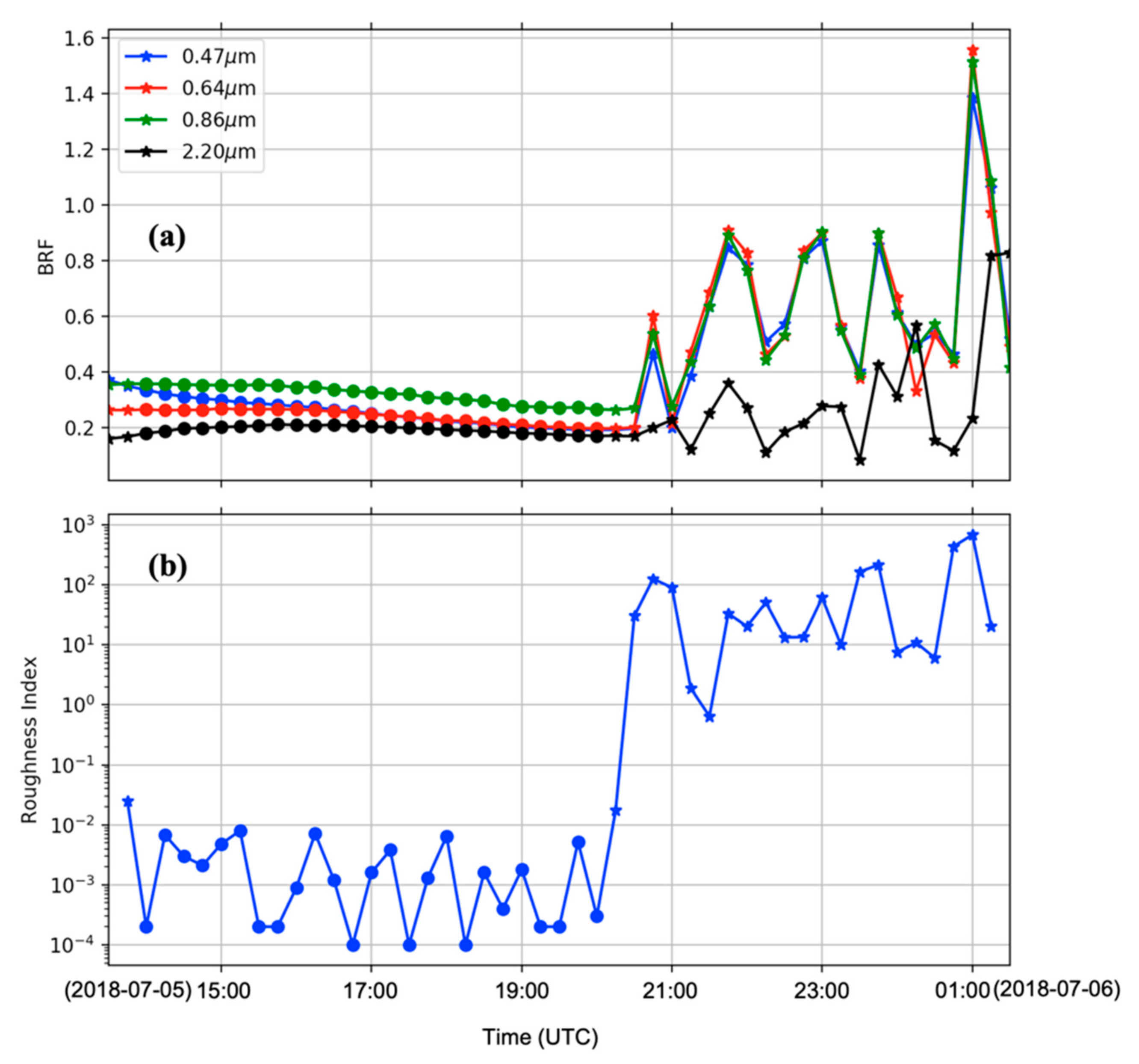
Figure 4 shows an example of the diurnal circle of the summertime TOA BRF at the Tucson site. As shown, the time series is very smooth in the (local) morning but becomes rough in the afternoon. Visual examination of the corresponding satellite images (not shown) indicated that the smooth time series were obtained under clear sky conditions while the increased variability in the afternoon corresponds to emerging clusters of cumulus in the sky.
The strong disparity between the smooth and the rough segments of the time series of TOA BRF is not unique to the Tucson site but observed everywhere across the domain, reflecting a key fact about the diurnal variability in the measured TOA BRF. Except for anomalous events (e.g., land clearing, snow storms, etc.), land surface structures and properties vary little on sub-daily time scales. Under clear-sky (cloud-free) conditions, variations in the reflected radiances (and the corresponding reflectances) are mainly regulated by the changing positions of the sun in the sky and thus are a smooth function of solar (and satellite) angles. Inversely, if the time series of radiance/reflectance change significantly at short (~10-min) time steps, they very likely indicate varying atmospheric conditions under the disturbances of, for instance, passing clouds or shadows. Therefore, the smoothness and roughness of the observed diurnal TOA BRF variations give us a handy tool to filter cloud-contaminated data and identify potential clear-sky measurements.
We devised a Roughness Index (RI) based on the second derivatives of time series to evaluate the smoothness/roughness of the diurnal variations in TOA reflectance. Mathematically, the second derivatives of a curve are closely related to its curvatures and thus commonly used to measure the roughness of curves [
50]. Because we are mainly interested in the magnitudes of the changing rates/curvature, we defined the RI as the squares of the derivatives:
where
is the TOA BRF of a given spectral band,
is the time step (in minutes), and
c is a constant scaling factor.
By Equation (3), the roughness index calculates how the TOA BRF at a given time step (
) deviates from the arithmetic mean of the preceding and the following measurements (
). The greater the deviation is, the larger the roughness index is. We can thus use a threshold,
RIthresh, to determine if the data were acquired under cloudy/unstable atmospheric conditions. In this study, we chose the scaling factor
c to be
so that
RIthresh is 1. An example of the roughness indices corresponding to the time series of TOA BRF at the Tucson site is presented in
Figure 4. As shown, the roughness indices are below 0.1 in the morning but above 1 in the afternoon, clearly indicating the distinction between the smooth and the rough segments of the time series.
The roughness index occasionally can have values lower than
RIthresh by chance (
Figure 4). Therefore, we tightened our criteria for potential clear-sky observations to be consecutive low
RI values at three or more timesteps. Additionally, because different spectral bands may be sensitive to different atmospheric or surface disturbances (e.g., cirrus or mist), we calculated the roughness indices for all reflective bands for data screening. We emphasize that (consecutive) low roughness indices are only a necessary, but not a sufficient, condition for detecting clear atmospheric conditions. Smooth TOA BRFs could result from large persistent cloud cover or sunglint over oceans. In cold seasons, we also want to differentiate snow-free and snow-covered surfaces. We need other tools (e.g., cloud tests based on temperature or brightness) to fulfill these tasks, which we will describe later in the paper. Nevertheless, the smoothness/roughness test of the diurnal variations in TOA BRF adds a new gadget to our toolbox to address these challenges.
2.5. Atmospheric Correction on Clear Days
Let us first consider atmospheric correction for the easier case when the sky is mostly clear during the day.
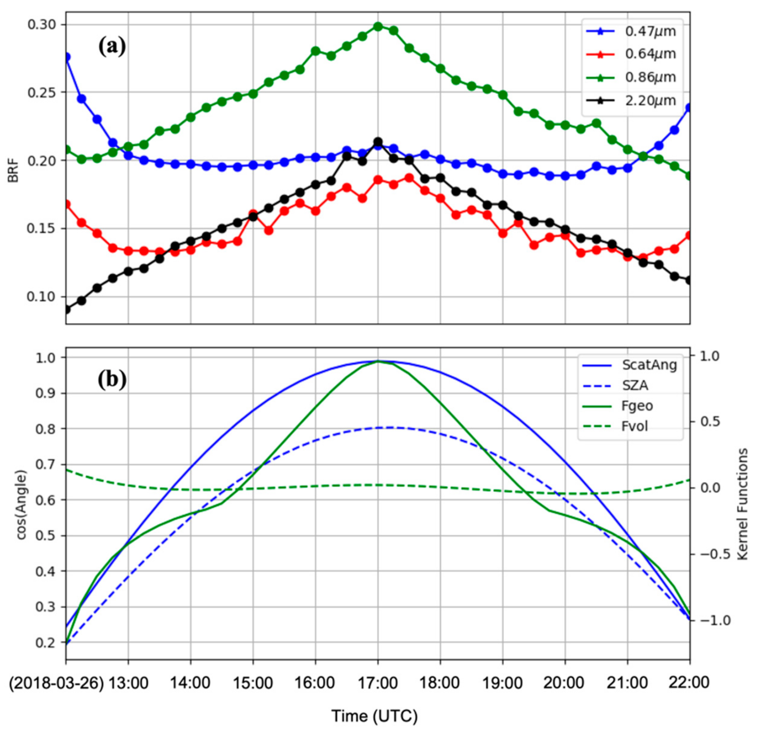
Figure 5 shows the TOA BRF of four Visible to Short-Wave Infrared (VSWIR) bands (0.47, 0.64, 0.86, and 2.20 µm) on 26 March 2018 at the GSFC site, where the time series are mostly smooth based on the roughness index criteria. The diurnal cycles of the reflectances reveal certain patterns. For bands of shorter wavelengths (e.g., 0.47 µm), the time series tend to show a “bowl” (or “cup”) trajectory: the TOA BRFs are as high as ~0.28 earlier in the morning, decrease to ~0.2 during the course of the day, and increase to ~0.25 later in the afternoon. This characteristic pattern reverses as the wavelength of the spectral bands increases. For the 2.20 µm band, for instance, the TOA BRF peaks at ~0.21 during the day and decreases to ~0.1 earlier in the morning or later in the afternoon, showing a “bell” (or “cap”) shape.
The TOA BRF patterns shown in
Figure 5 reflect the relative balance between the scattering and the absorption of photons in the atmosphere and the surface media (e.g., canopy), and are also related to the illumination-view geometry at the site (see below). Indeed, these patterns reflect a phenomenon known as the “hot-spot” effect, which occurs when the solar illumination direction and the satellite view direction coincide [
51]. For geostationary sensors, the hot-spot phenomena are most evident in March and October over CONUS [
52]. Shown in the bottom panel of
Figure 5, the scattering angle approaches 172° around 17:00 UTC, indicating the close approximation of the positions of the Sun and the satellite in the local sky. This timing corresponds to the substantial rises (i.e., the “hot-spot”) in the TOA BRFs in the longer-wavelength bands.
Figure 5 shows also that the hot-spot effects are partially captured by the geometric optical kernel (Fgeo) of the RTLS model. The volumetric kernel (Fvol) shows a “bowl” shape similar to the diurnal trajectories of the Blue (0.47 µm) and the Red (0.64 µm) bands, suggesting stronger scattering at larger solar zenith angles (
Figure 4).
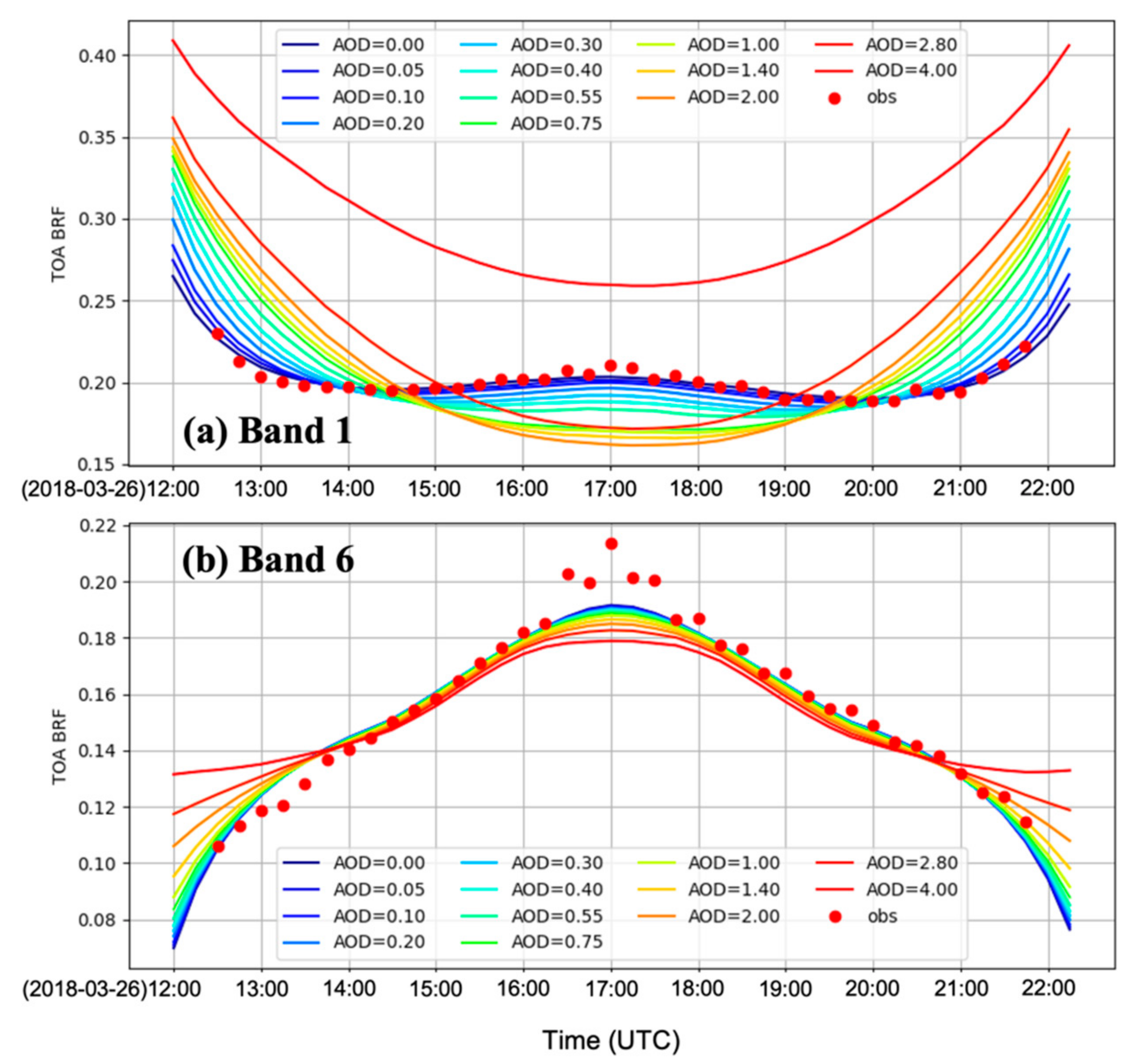
We used the MAIAC RTM to simulate the identified diurnal variability in the clear-sky TOA BRFs. We ran the RTM at 13 AOD levels ranging from 0 to 4.0 and, for each AOD level, used a gradient-descent approach to optimize the surface reflectance BRDF parameters (Equation (1)) so that the simulated TOA reflectance (Equation (2)) best matches the observations. To ensure that the results are physically justifiable, we imposed further constraints on the retrieved RTLS parameters (i.e., ) so that they are non-negative. We evaluated the performance of the optimization by calculating the root-mean-square-error (RMSE) statistics.
Figure 6 shows the simulation results for the Blue band (0.47 µm) and the SWIR band (2.20 µm) with the RTLS BRDF model, which well capture the observed diurnal cycles of the TOA BRF for both bands. For AOD levels from 0.0 to 0.1, the RMSE statistics are ~0.006 for the Blue band and ~0.007 for the SWIR band, suggesting that the model simulation errors are generally less than 5% of the observed TOA BRF. The errors between the simulation and the observations apparently increase when the AOD increases. The spread of the model simulations at high AOD levels is particularly wide for the Blue band. The spread of the SWIR simulations is mostly discernible early in the morning or late in the afternoon. All these results suggest that the atmospheric aerosol loading is low at the GSFC site on the particular day.
The simulation results shown in
Figure 6 indicate that, with appropriate RTLS parameters and AOD values, the MAIAC RTM can accurately simulate the observed diurnal variability in the TOA BRFs for all spectral bands in the visible to short-wave infrared range. In other words, surface reflectance on diurnal time scales is a smooth function of the illumination-view geometry, which can be accurately represented by the RTLS model to the extent of the observed (solar and satellite) angular space. On the other hand, though a bit unfortunate, the solutions of appropriate AOD values and RTLS parameters are not unique. As shown in
Figure 6, for any AOD value from 0 to 0.1, there exist reasonable RTLS parameters that allow the RTM to successfully simulate the observed TOA BRF. Therefore, we calculated the weighted mean of AOD values that have the lowest RMSE values and satisfy certain other criteria (see below) as the best estimate of mean AOD for the given day. We also used the range of the most plausible AOD levels as a metric to evaluate their uncertainties.
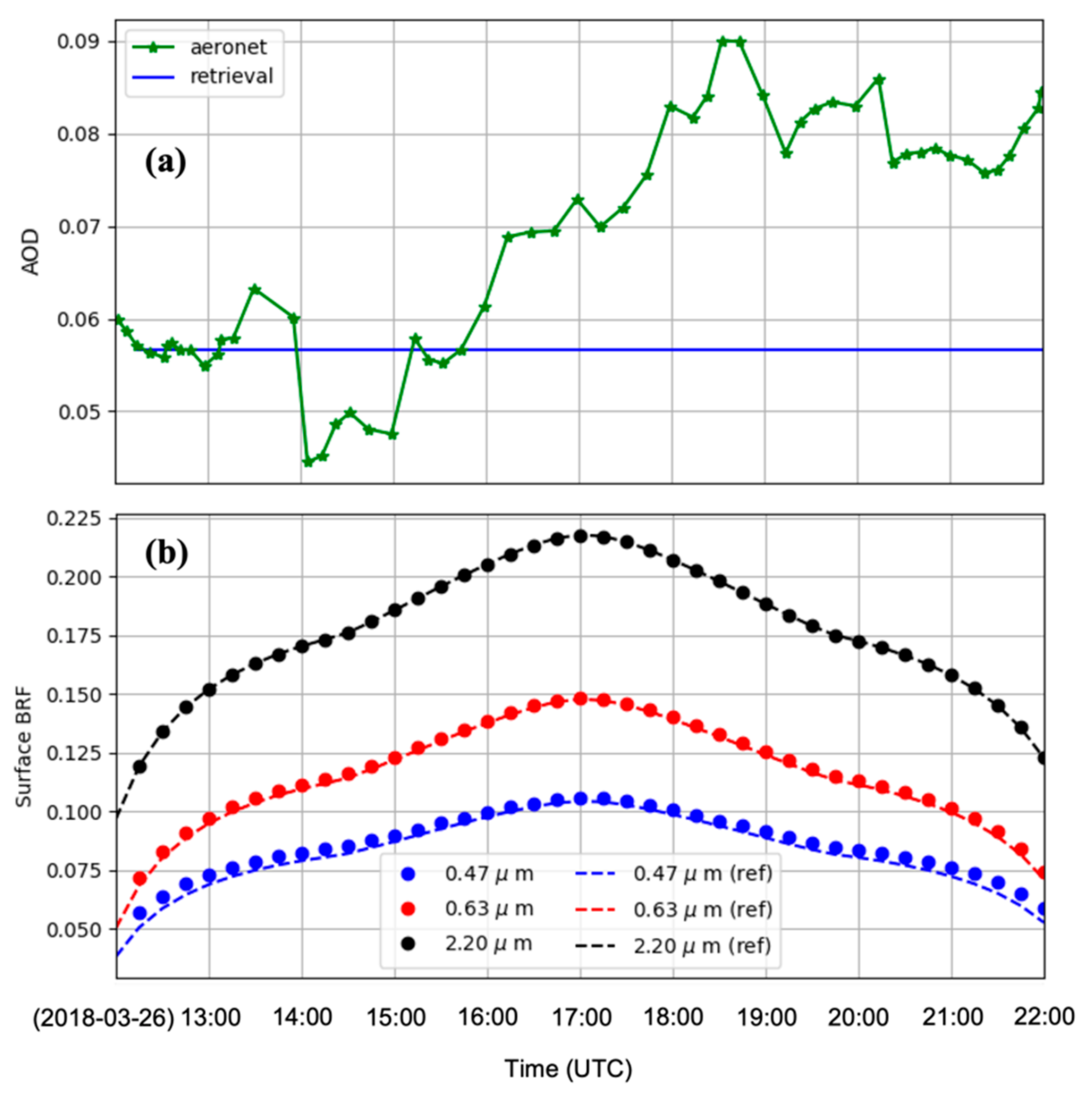
Figure 7 shows the atmospheric correction results of the time series shown in
Figure 5 with the RTM simulations presented in
Figure 6. The retrieved AOD value generally agrees with the ground-based measurement, though our algorithm has neglected the diurnal variations in AOD. This is a compromise made for greater degrees of freedom in our analysis. The retrieved diurnal cycles of the Surface BRF (SR) clearly show the regulation of the RTLS model. They all show a “bell” shape, though to various amplitudes, reflecting the influence of the geometric optic kernel function (
Figure 5). These results indicate that the angular dependence of the surface reflectance (i.e., the BRDF effects) is a key source of information for us to perform atmospheric correction. Because there is no ground-measured surface reflectance (at satellite pixel scales) available to validate the retrieved results, we used the AERONET-measured AOD as an input to the MAIAC RTM and derived a set of “reference” surface BRFs following a common procedure in the literature [
34]. This approach largely eliminates the uncertainties associated with the atmospheric optical properties, and thus the reference data are considered as the best proxy of the “true” surface BRF. Comparing the retrieved surface BRF with the corresponding reference data indicates a high degree of agreement (
Figure 7). Although the reference data are not ground truths but model results, the consistency between the two sets of results (
Figure 7) confirms that our retrieval algorithm (for surface reflectance, in particular) is robust. The corresponding RTM simulations with the Lambertian surface model (not shown) were found to be less optimal than the RTLS counterparts.
2.6. Atmospheric Correction on Partially Clear Days
Fully clear days like the one shown in
Figure 5 are relatively rare, especially in cloudy regions like the tropics. More frequently, the sky will be clear for a few hours and then covered by clouds, or vice versa. The number of clear observations we can obtain on partially clear/cloudy days can be much less than those shown in
Figure 5. The fewer clear observations present additional challenges to atmospheric correction. They reduce the degrees of freedom in the empirical analysis such that the results become unreliable (e.g., overfit) at a certain point. More importantly, retrievals with fewer observations are typically associated with higher uncertainties. The latter can be understood by the model simulations shown in
Figure 6. The TOA BRFs simulated with a wide range of AOD levels (0–0.55) have similar trajectories between 15:00 UTC and 19:00 UTC (roughly local time 10 a.m. to 2 p.m.) at the GSFC site (
Figure 6). If the only clear observations were restricted in this time window on that day, the upper bound of acceptable AOD levels that allow the MAIAC RTM to reasonably approximate the observed TOA BRF could be increased up to 0.55 with suitable surface RTLS parameters. Therefore, we need a different approach to perform atmospheric correction on partially clear days.
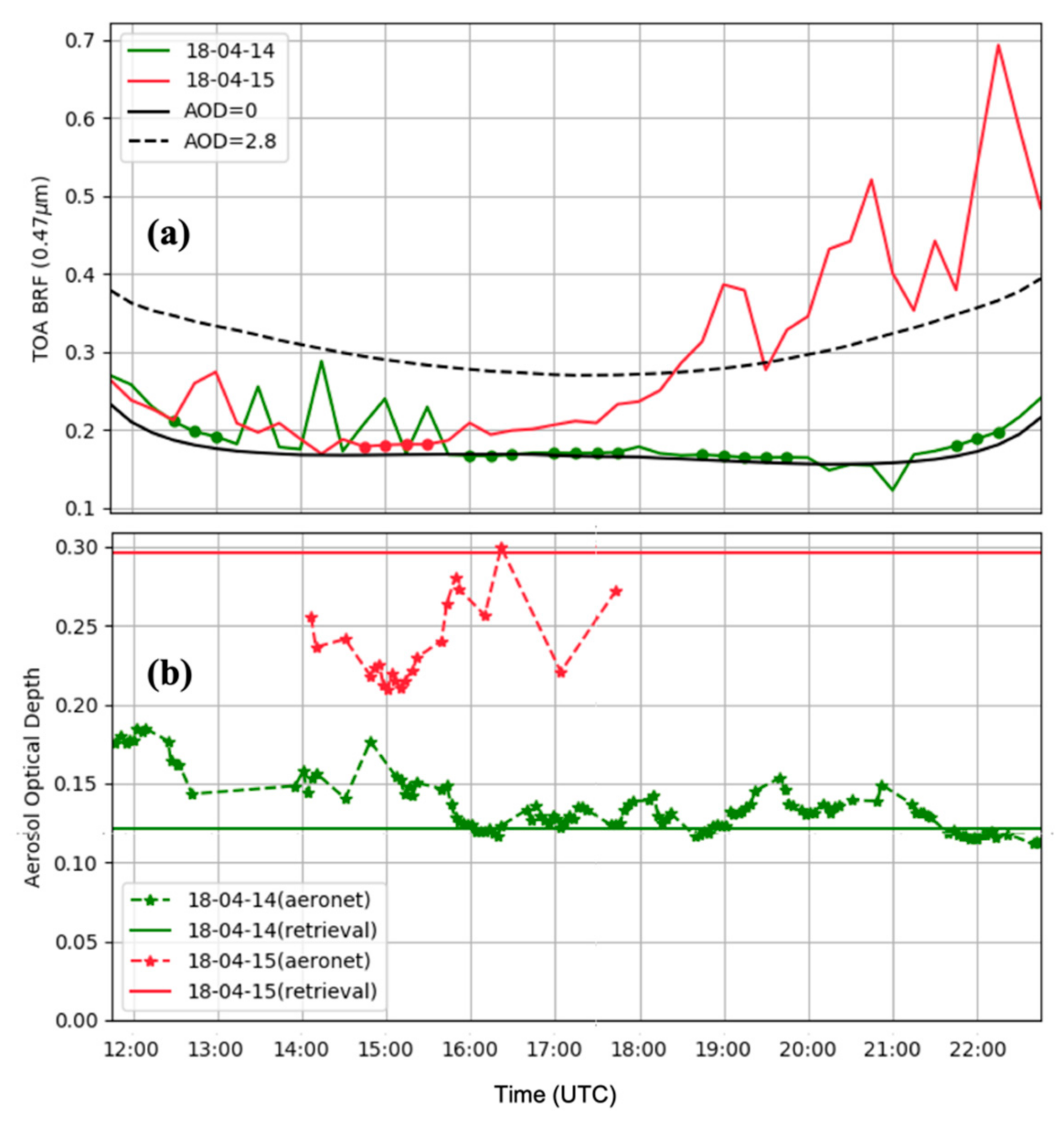
A natural strategy to address the challenge of partially clear days is to leverage the retrievals from the preceding (or adjacent) days as prior information in the analysis. To illustrate, the top panel of
Figure 8 shows two diurnal time series of TOA BRFs observed at the Key Biscayne AERONET site on 14 and 15 April 2018. Based on the roughness indices and other tests, there are only four reliable clear observations on 15 April at the site (
Figure 8), making it impractical to perform the full retrieval algorithm on that day. Fortunately, there are more than a dozen cloud-free observations on 14 April (
Figure 8), which allow us to successfully retrieve the surface RTLS parameters. The trajectories of the clear-sky observations on both days appear to be consistent (
Figure 8), suggesting that the surface reflective properties did not change much between the two days. We can therefore use the RTLS parameters estimated on 14 April as the prior information, with some necessary adjustments (see below), to estimate the AOD level on 15 April. The bottom panel of
Figure 8 shows that the retrieved AOD values closely match the corresponding ground measurements.
There may be multiple days before a full set of RTLS parameters can be independently retrieved. It is thus necessary to adjust the prior RTLS information before performing partially clear-day retrievals. One approach to do this is to allow the magnitudes of the RTLS parameters to change but assume the BRDF shape to be stable. That is, we represent the new RTLS parameters (at time
t) as the product of the prior ones (at time
t − 1) and a single scaling factor (
),
or more explicitly
In this way, we only need to estimate the scaling factor (
) from the observations and therefore save the degrees of freedom of the analysis. This method is often referred to as the Vermote–Justice–Bréon (or simply VJB) approach after the authors’ 2008 paper [
53].
A convenient way to estimate the scaling factor for all the bands can be achieved with the spectral dependency assumption mentioned in the Introduction, which suggests that the ratios between the directional reflectances of different spectral bands are relatively stable [
19]. Under this assumption, variations in the scaling factors among different spectral bands are negligible and thus we only need to estimate one scaling factor for all the bands. We chose the SWIR band to estimate the scaling factor because this band is less affected by AOD variations due to its longer wavelength.
We notice that the VJB assumption (i.e., the BRDF shape does not change) is a very strong constraint on the retrieved surface reflectance, which should be gradually relaxed with the elapse of time between adjacent partially clear-day retrievals. For this purpose, we compiled the surface reflectance in the past few days (up to 32 cloud-free observations) and re-estimated the RTLS parameters from the composited time series. The re-estimated RTLS parameters were deemed the “posterior” results and used to calculate the surface reflectance.
Figure 9 shows the retrieved surface reflectances of the Blue and the SWIR bands at the Key Biscayne site on 14–16 April 2018. The results generally suggest that the BRDF at the site has a relatively strong geometric-optics component such that the reflectances decrease substantially (>30%) at large solar zenith angles. The surface reflectances on 15 April closely follow those of 14 April, reflecting the influence of the latter (as the prior estimates) on the retrieval results on (partially) cloudy days. Interestingly, we see that the Blue-band reflectances on 15 April are slightly higher than those on 14 April while the corresponding SWIR reflectances are slightly lower. This implies small variations in the ratio between the two bands. The surface BRDF on 16 April, which was independently estimated (and the retrieved AOD is highly consistent with AERONET measurements), shows more discernible differences from the preceding days. In particular, the SWIR band reflectance decreases (−5%) around local noon but increases (up to ~30%) in the morning and the afternoon, indicating variations in the ratios between the Blue and the SWIR bands on diurnal scales. Such BRDF changes on successive days emphasize the importance of frequently updating the surface RTLS parameters with new observations, especially when surface changes are detected (see below).
2.7. Snow and Cloud Detection
Although (land) surface properties in general do not rapidly change, rapid changes could happen with natural or anthropogenic disturbances, including snow, wildfire, agricultural harvesting, forest clearcutting, and so on. In particular, snowfall occurs commonly over vast regions outside the tropics (and the subtropics) during the cold seasons and can induce significant changes in surface reflectance overnight.
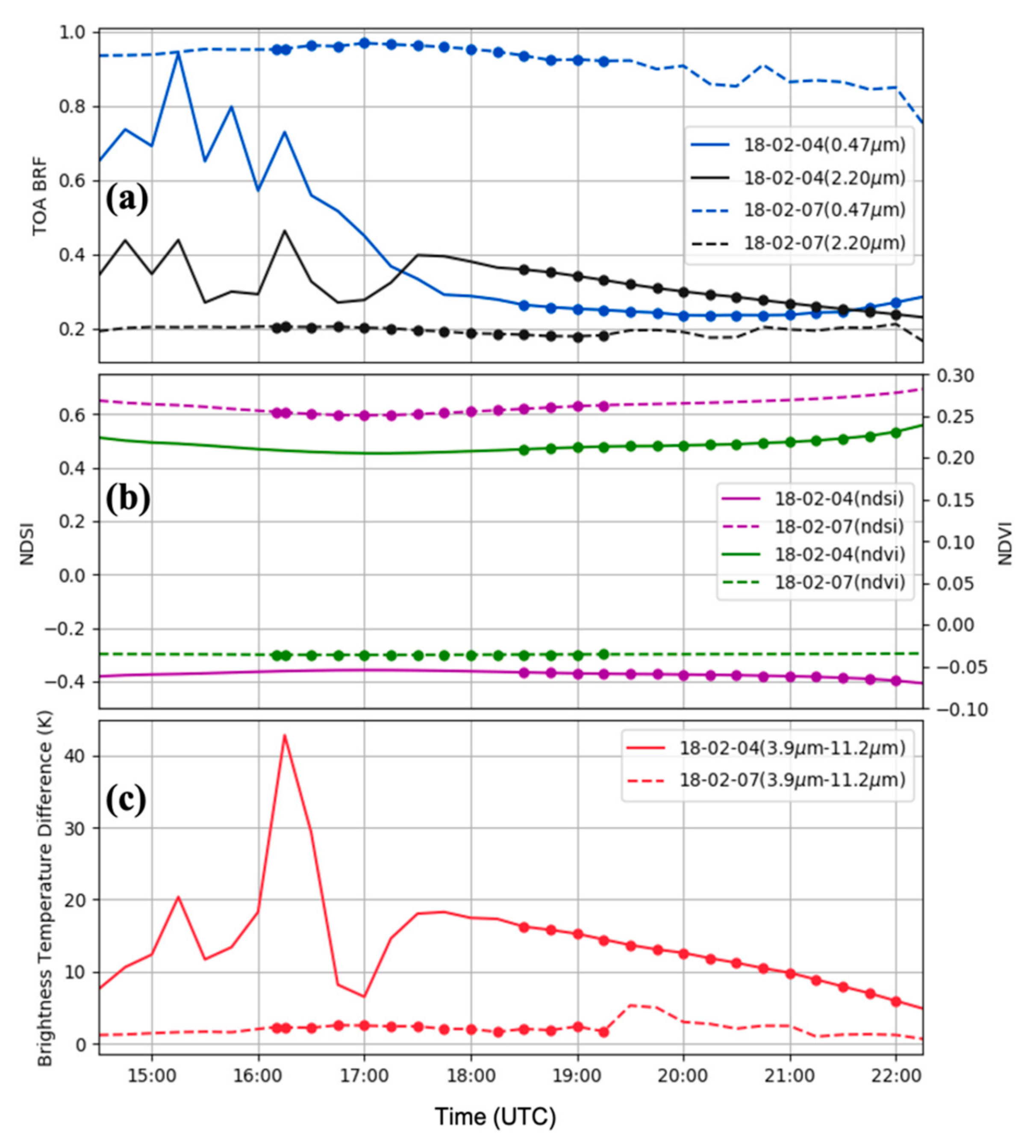
Figure 10 shows an example observed at the SMEX/Ames (Iowa) AERONET site between 4 and 7 February 2018 (where the two days of the 5th and the 6th are totally cloudy). In only a couple of days, the Blue BRF increased from ~0.25 to ~0.9, indicating significant brightening of the surface in the visible spectral range. In comparison, the SWIR BRF decreased (“darkened”) from above 0.3 to below 0.2. The diurnal time series of the SWIR BRF also flattened on 7 February, showing much less sensitivity to the illumination geometries during the course of the day as compared with the snow-free case on 4 February.
We used a set of spectral variables/indices to detect surface snow and discriminate between snow and persistent cloud cover, including the Normalized Difference Vegetation Index (NDVI), the Normalized Difference Snow Index (NDSI), and the Brightness Temperature Difference between the 3.9 µm and the 11.2 µm bands (dBT4-11). They are calculated as follows:
where
and
represent the reflectance (or reflectance factor) and the brightness temperature at the spectral band or wavelength
, respectively. Note that because the GOES16/17 ABI does not have a Green band, we used the Red band in calculating the NDSI.
In general, NDVI values are high (>0.7) over densely vegetated pixels, low (<0.3) over bare soils, and can even be negative over snow pixels [
54]. The NDSI behaves in an opposite manner to the NDVI, having positive/high values (up to 1.0) over snow cover but negative/low values over common snow-free surfaces [
55]. The MAIAC algorithm uses a NDSI threshold of 0.3–0.4 for snow detection, where pixels with a NDSI exceeding the threshold are considered to be potentially covered by snow. However, this criterion alone is not sufficient to make the final classification as high NDSI values can also result from ice clouds [
56,
57]. The brightness temperature contrast test (dBT4-11) was thus used to help solve the problem. During the day, the 3.9 µm band of the ABI instrument senses both reflected solar radiation and Earth-emitted radiation. Because water and small ice crystals in the clouds are more effective in reflecting the 3.9 µm infrared radiation than the large ice crystals in the snow, this leads to a higher thermal contrast in clouds than surface snow [
1]. We used a dBT4-11 threshold of ~5 K in our algorithm, where bright pixels with a high NDSI value and a low thermal contrast dBT4-11 value are reliably classified as snow cover. The effectiveness of these tests is illustrated in the middle and bottom panels of
Figure 10. From the 4 to the 7 of February at the SMEX/Ames site, NDVI values dropped from 0.22 to −0.02, the NDSI increased from −0.4 to 0.6, while the dBT4-11 remained less than 3 K on the 7th, especially for the identified clear-sky data points (
Figure 10). These results together indicate that the detected surface changes were induced by snow, likely precipitated on 5 and/or 6 February 2018 in this region, which is consistent with visual examination of the corresponding satellite images (not shown).
Compared with the large contrast between snow-covered and snow-free surfaces as shown in
Figure 10, the transition states, such as melting snow or partial snow cover, are more challenging to detect. For this purpose, we refined the snow tests by evaluating changes in NDVI and NDSI between the observations and the expectation (or the prior information), that is,
where the prior NDVI/NDSI indices are calculated with the previously retrieved results. The pair of differential indices turns out to be very useful in detecting subtle but important surface changes.
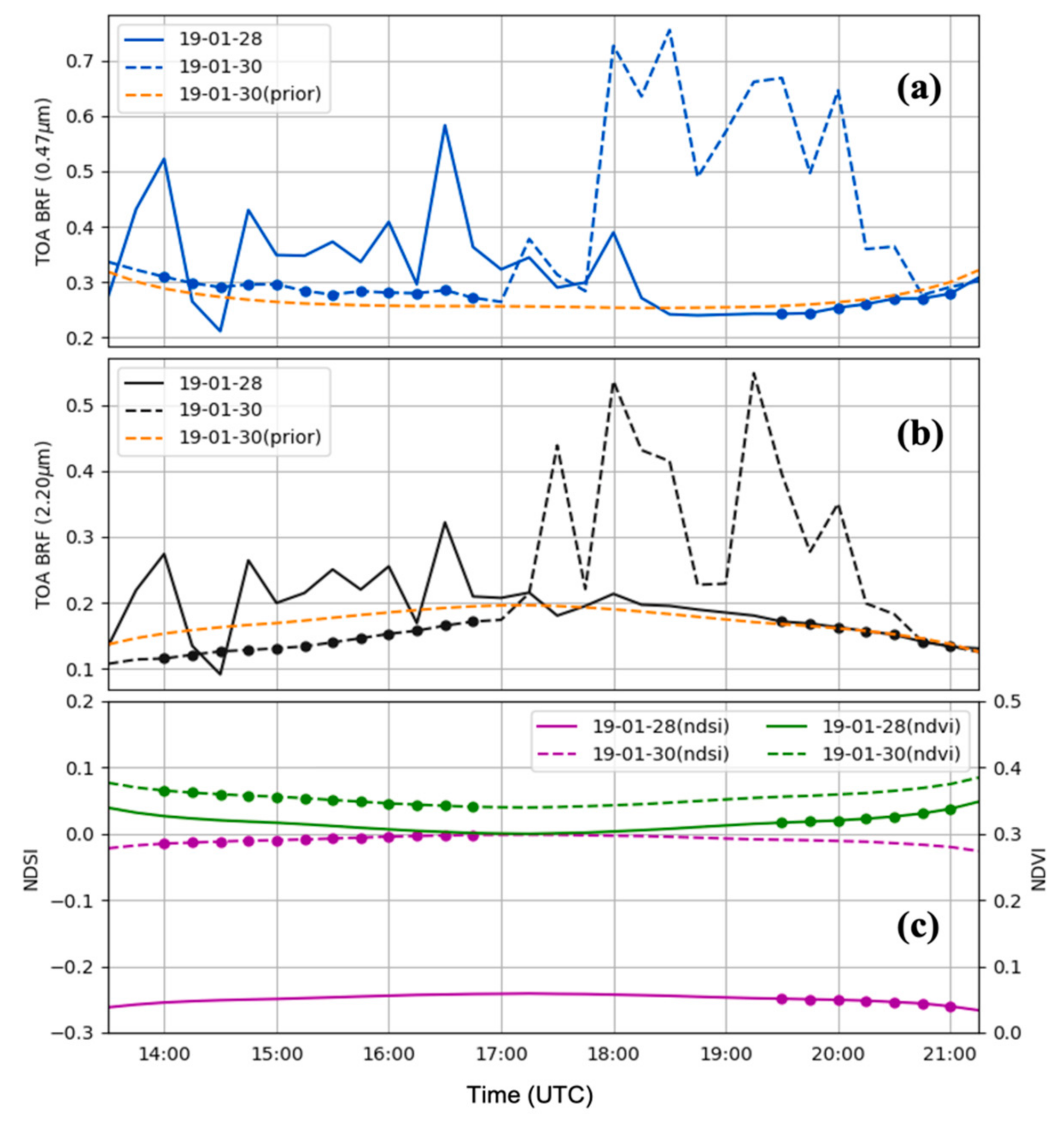
Figure 11 shows an example of TOA BRFs observed at the GSFC site on 28 and 30 January 2019 (the 29th is totally cloudy). At first sight, the clear-sky observations on the 30th appear to be consistent with those of the 28th, suggesting similar surface conditions between the two days. However, when we compare the observations of the 30th with the corresponding prior estimates, which were simulated with the RTLS parameters retrieved (or updated) on the 28th and an initial estimate of AOD (0.05), it becomes clear that the observed BRFs of the Blue band (and other visible/infrared bands) are consistently higher than the prediction while those of the SWIR BRFs are lower (
Figure 11). If we estimate the surface reflectances of the Blue band from the SWIR band using the VJB approach described in the preceding section, they will be under-estimated, and the differences between the observed and the simulated Blue-band TOA BRFs will be further over-estimated. The enlarged discrepancies have to be compensated for by increased scattering of the atmosphere, which ultimately leads to large positive anomalies in the retrieved AOD (not shown). Fortunately, such biases are captured by the dNDSI test. Shown in the bottom panel of
Figure 11, the NDSI values on 28 January are about −0.25 on average and jump to about −0.05 on the 30th. Although the NDSI values are still low and the corresponding changes in NDVI are small (
Figure 11), this magnitude (~0.24) of the dNDSI alone cannot be easily dismissed. Visual examination of the satellite images indicated that partial snow cover is most likely the culprit in this example. Our algorithm currently classifies such cases as partial cloud or snow, depending on the context of a few other criteria (e.g., temperature). In any case, subtle surface changes of this kind should be separated from the normal conditions and the dNDSI/dNDVI tests serve the task well.
3. Results
We ran the GeoNEX-AC algorithm at the selected AERONET sites (
Table 1) for a two-year period from 1 January 2018 to 31 December 2019 and compared the retrieved results with the corresponding ground observations.
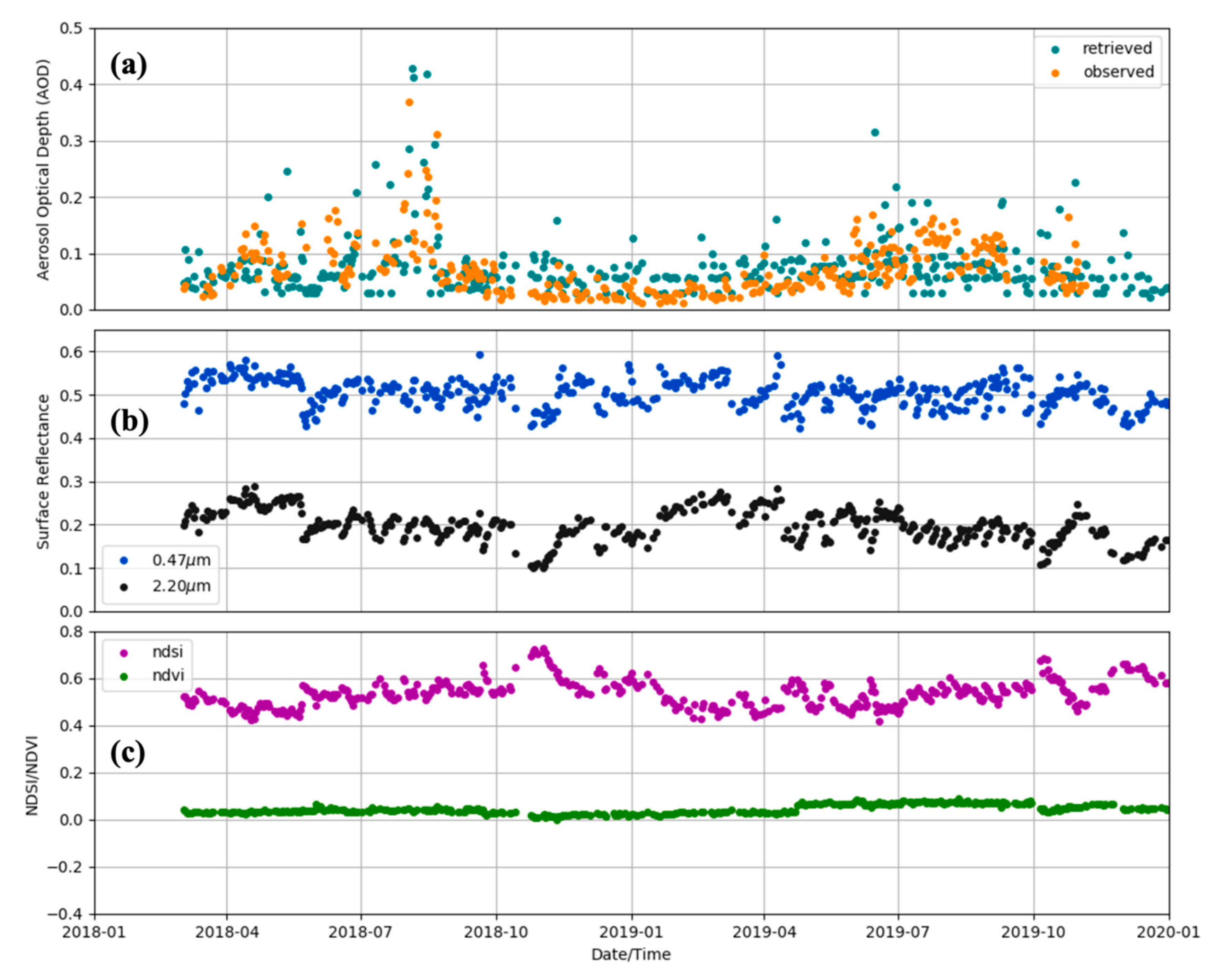
Figure 12 shows the daily averaged results retrieved at the White Sands site compared with AOD observations measured at the nearby White Sands HLSTF site. This site was chosen as an example because it represents a few challenges for traditional atmospheric correction algorithms. The surface is very bright in the visible spectral range at the site. The Blue-band surface reflectance is ~0.5 (
Figure 12), while it is typically less than 0.1 at vegetated surfaces (see
Figure 7 and
Figure 9 for the cases of the GSFC and the Key Biscayne sites, respectively). This implies that the regulations of atmospheric aerosol loadings on the TOA BRFs are relatively weak as compared with variations in the surface reflectance. As a result, the retrieved AOD values are often associated with large uncertainties [
58,
59,
60]. In contrast to the bright visible bands, the reflectance at the SWIR band at the site is relatively low. The large positive contrast between the visible and the SWIR bands results in high NDSI values (0.4–0.6;
Figure 12), making it difficult to separate from clouds or snow in the cold season.
Because we ran our algorithm without prescribed prior information, the high brightness and high NDSI values confused the cloud/snow detection tests at the beginning of the run: the algorithm struggled to identify any clear or partially clear days for an elongated “burn-in” period of almost two months (
Figure 12). However, when the site was finally classified as a bright snow-free surface (with the help of temperature tests), the algorithm started to regularly and accurately retrieve AOD and surface reflectance for the remainder of the experiment. As shown, the retrieved AOD well captures the daily and seasonal variations in the corresponding AERONET observations (
Figure 12). The correlation and the RMSE statistics between the two time series are about 0.8 and 0.05, respectively, with the retrieved AOD being ~20% higher than the observations. The AOD retrievals, though not perfect, give us confidence in the retrieved surface reflectance, where ground observations at the spatial scales of satellite image pixels are difficult to obtain. Sensitivity tests of the MAIAC RTM indicate that the variations in surface reflectance induced by an AOD uncertainty of 0.05 are generally less than 0.01 at the Blue band and further decrease towards longer-wavelength bands. This level of uncertainty is relatively small compared with the retrieved daily/seasonal variations in SR shown in
Figure 12. In other words, the SR values retrieved from our algorithm are accurate and thus can provide a robust source of information to study the dynamics of surface processes (e.g., phenology) at daily to seasonal time scales (see below).
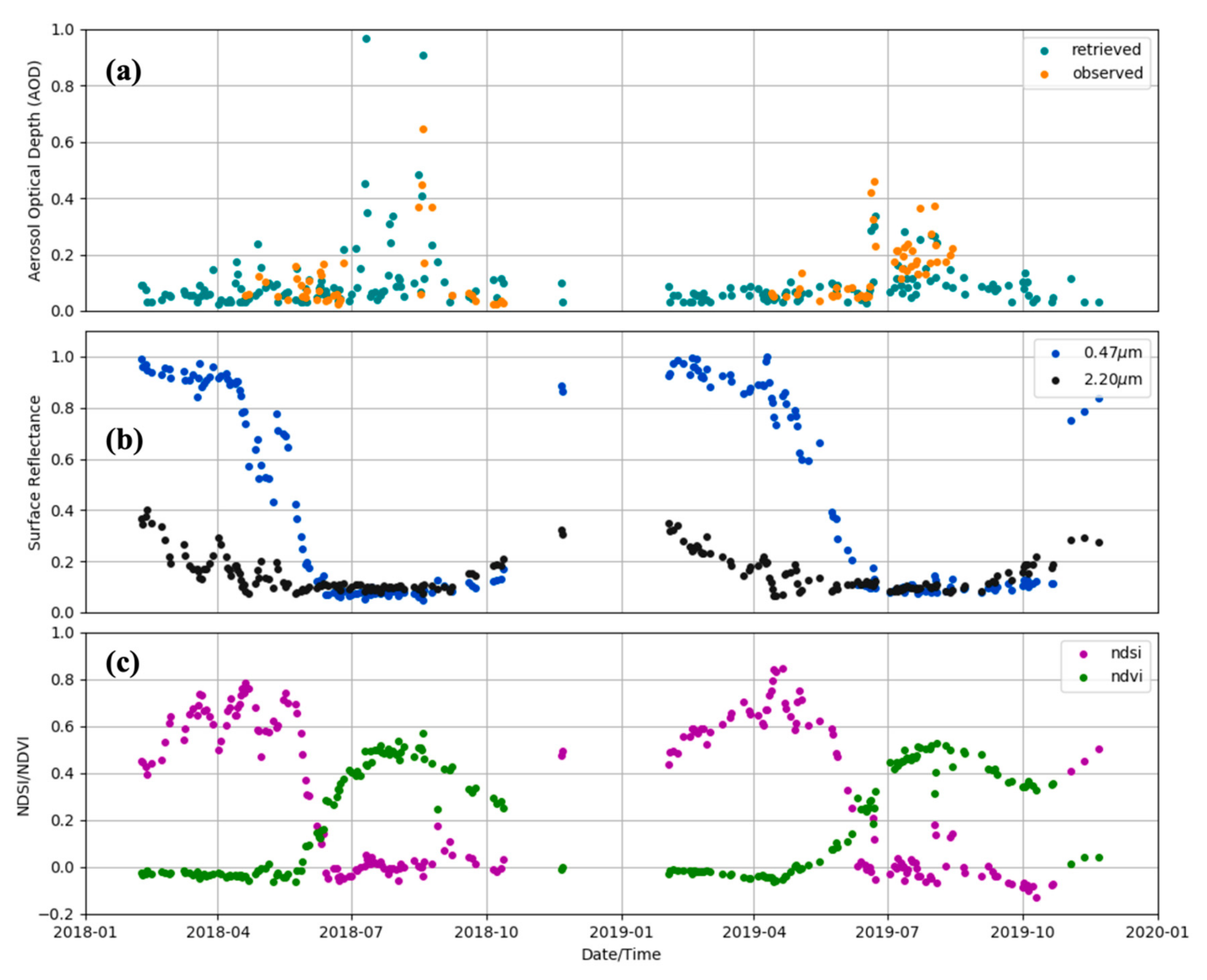
Figure 13 shows another challenging example at the Churchill AERONET site, which is located not far from the northmost boundary of the GeoNEX grid (60° N). Because the satellite zenith angle is large at this latitude, the data quality of TOA BRFs is more sensitive to changes in solar zenith angles and day lengths than at lower latitudes. As a result, few clear (or partially clear) days can be identified during the winter months (October to February of the next year) at this site (
Figure 13). For the rest of the months, the site is covered by snow until May when it starts to melt. By the end of June, the surface is largely snow-free. As shown, the Blue-band reflectance drops sharply from 0.8 to 0.1 between May and June (
Figure 13). The corresponding NDSI drops from 0.6 to about 0 while the NDVI increases from 0 to about 0.4 by the end of June. The increase in NDVI (or surface greenness) continues until it peaks in late July/early August, and then the trajectory reverses. By early October, the NDVI decreases to about 0.2 before the first snowfall of the next cold season (
Figure 13). As such, the phenological cycle and its interannual variations at the site are well captured by the retrieved time series of surface reflectance and vegetation/snow indices.
Figure 13 also shows that the retrieved AOD values are closely comparable to the in-situ measurements. The correlation and the RMSE statistics between the two time series are about 0.9 and 0.06, respectively, with the retrieved AOD being slightly (~10%) lower than the observations. It is important to notice that the retrieval algorithm correctly captures multiple large AOD anomalies caused by wildfires. The two clusters of AOD anomalies in August 2018 and June 2019, where corresponding AERONET observations are available, indeed reflect the influences of the Carr Fire in California (2018) and the Alberta Fire in Alberta, Canada (2019), where the smoke is transported by the atmospheric circulation thousands of miles across the continent. The other spike of AOD anomalies in July 2018, where no corresponding AERONET measurements are available, appears to have been induced by the smoke transported from the North Bay 69 fire in Temagami, Ontario. The successful detection of these events demonstrates the capability of our algorithm to distinguish smoke/heavily polluted air from other atmospheric disturbances (such as partial/sub-pixel clouds).
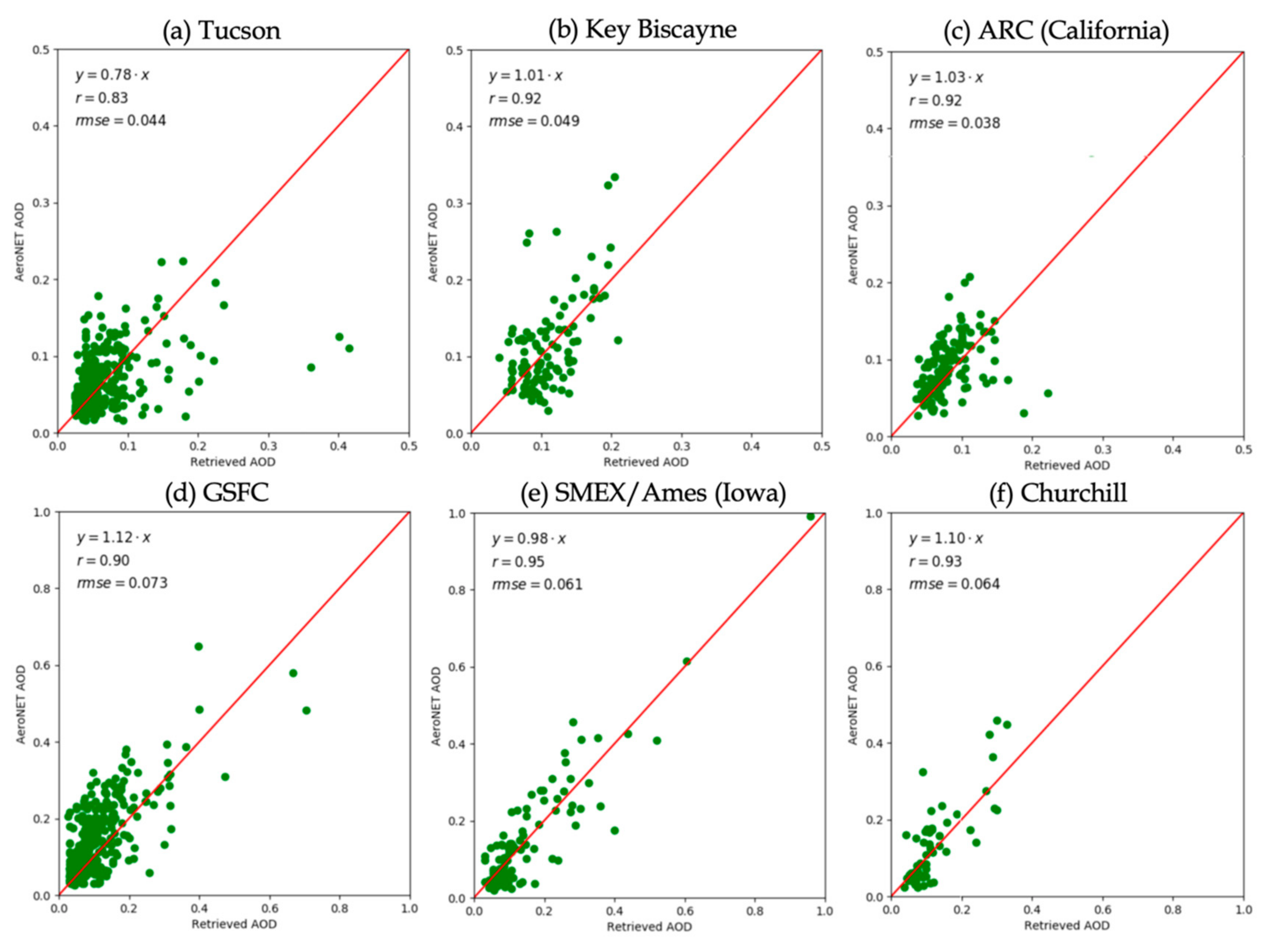
Figure 14 shows the comparisons of the retrieved and the observed daily AOD at the rest of the selected AERONET sites. The results are consistent with those described for the White Sands and Churchill sites. In particular, the correlations between the retrievals and the observations are greater than 0.9 at the Key Biscayne, ARC, GSFC, and SMEX/Ames sites, where the regression coefficients are also very close to 1 (
Figure 14). The corresponding statistics are less optimal at the Tucson site, mostly likely induced by the fact that the surface is brighter at the semi-arid site. On the other hand, the RMSE values of the comparisons are lower (~0.04) at the Tucson and ARC sites but slightly higher (~0.06–0.07) at the GSFC and SMEX/Ames sites, where the AOD values also cover a higher range (
Figure 14). Such inter-site differences likely reflect the spatial pattern of mean AOD levels over the United States, which are typically higher over the East Coast than the West [
61]. Overall, the results presented in
Figure 14 suggest that our AOD retrievals have similar, if not better, accuracy and precision as the latest MODIS products [
60]. We recognize that our algorithm retrieves daily mean AOD levels while MODIS products reflect a “snapshot” of the AOD at the measurement time. Therefore, the two products may not be directly comparable. Because this paper mainly focuses on the algorithm’s development, we have not conducted comprehensive intercomparisons between the GeoNEX level 2 products and the corresponding MODIS (or other satellite) products, which we plan to report in the future.
Finally, and importantly, a key feature of the surface reflectance and BRDF information retrieved by our algorithm on clear days is that they do not depend on conventional assumptions of stable spectral band ratios [
19]. Therefore, these results provide independent data sources to examine such assumptions.
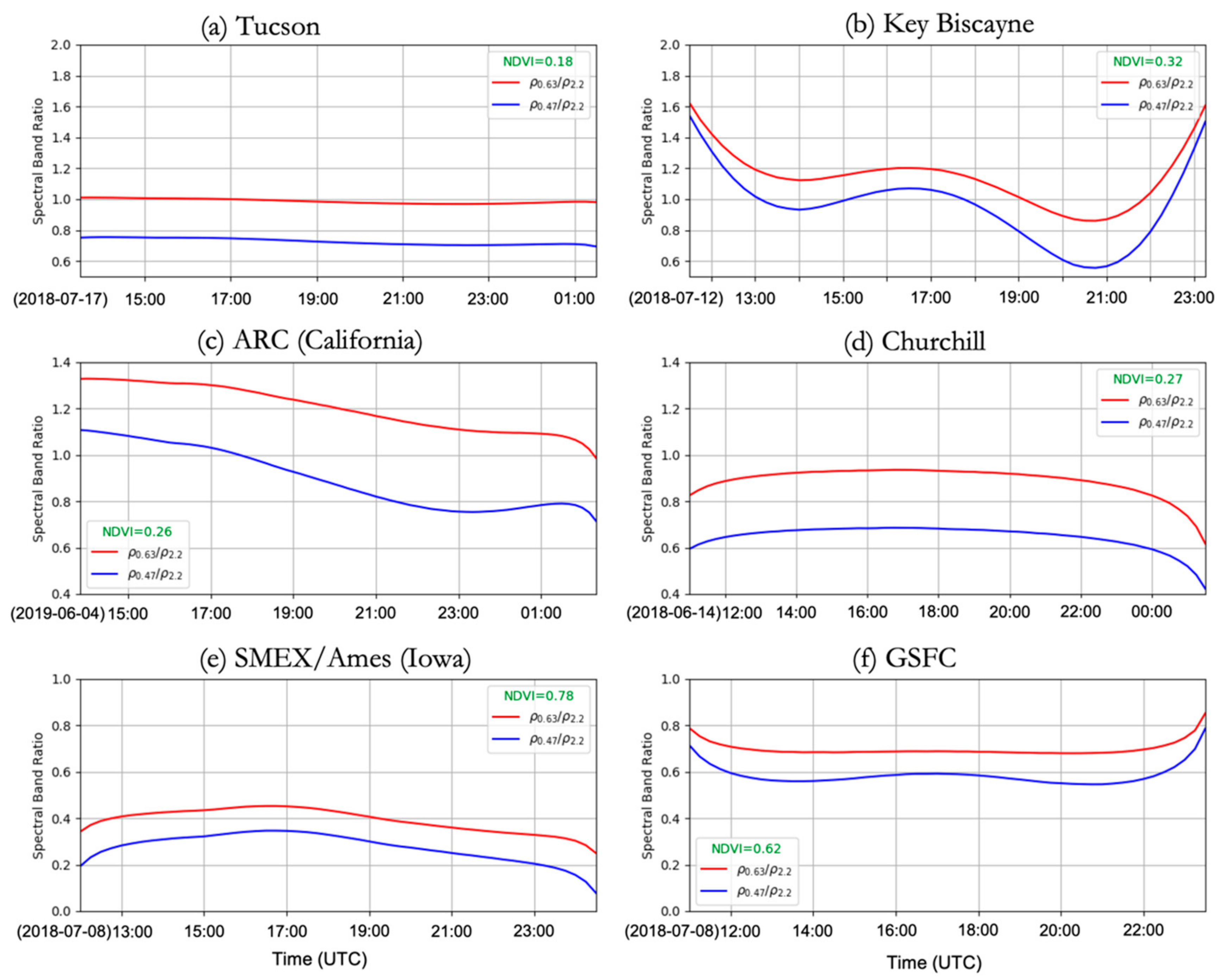
Figure 15 shows the diurnal cycles of the ratios between the Blue/Red bands and the SWIR band, respectively, at the testing AERONET sites on cloud-free days when the atmosphere is clear and the retrieved AOD values closely match the ground observations. Overall, we see a diverse range of variabilities in the band ratios in both spatial (between-site) and temporal (diurnal) dimensions. For instance, the mid-day Blue-to-SWIR ratio is above 1.0 at the Key Biscayne site but is only ~0.3 at the SMEX/Ames site. Their diurnal variations also show different patterns, which can be flat (Tucson), bowl-shaped (Key Biscayne and GSFC), bell-shaped (Churchill and AMEX/Ames), or rather asymmetric (ARC). The reasons for the variations in the band ratios are complex, involving illumination-view geometries, land cover types, surface heterogeneity, and other factors [
20,
62]. For instance, the relatively large Blue-to-SWIR ratios at Key Biscayne are likely influenced by the coastal location of the site, where the reflectance in the SWIR range is negligible over the adjacent waters. The relatively low band ratios at SMEX/Ames likely reflect that the site is densely vegetated, which is also suggested by the corresponding NDVI value (0.78;
Figure 15). Indeed, the mid-day band ratios at the SMEX/Ames site are close to that originally suggested by the literature for dense vegetation (0.25/0.5 between the Blue/Red and SWIR bands) [
19]. However,
Figure 15 emphasizes that the spectral band ratios change significantly over different land-cover types. Even for the densely vegetated site (SMEX/Ames), the ratios can change by 50% at large sun (zenith) angles (
Figure 15).
Although the spatiotemporal variability in spectral band ratios is complicated and difficult to describe analytically, such diurnal variability at individual sites is continuous (
Figure 15) and varies smoothly on consecutive days (
Figure 9). It is thus a legitimate approach to dynamically maintain the diurnal cycle of spectral ratios at each pixel for atmospheric correction in the subsequent time steps, which is a key feature of the MAIAC algorithm [
11,
16]. As the archive of (third-generation) geostationary data grows, we expect to collect more and more clear-day observations to derive independent diurnal cycles of the spectral band ratios to study their spatial and temporal (e.g., seasonal and annual) variations.
4. Discussion
A limitation of the current GeoNEX-AC algorithm is that it retrieves only daily mean AOD. This compromise, as stated before, was made to save the degrees of freedom in the statistical analysis for atmospheric correction on individual clear-sky days. Intuitively, we may wonder whether the constraint on degrees of freedom may be relaxed. For instance, because surface optical properties do not change much at the scale of a few days, we may use the BRDF parameters estimated from preceding days as the (a priori) inputs to the RTM to simulate the TOA BRF at every time step and thus retrieve time-specific AODs. However, succeeding in this task requires a deeper understanding of the propagation of uncertainties in the surface BRDF and atmospheric AOD, as well as their influences on the TOA BRF.
Neither the RTM nor the input data are perfect. In general, RTM simulations with the reference surface BRDF (RTLS) parameters and the AERONET-observed AOD are not able to fully replicate the observed TOA BRF variations. Aside from the uncertainties associated with the TOA BRF, such model-observation discrepancies can be induced by the truncation errors of the surface BRDF because the three kernels of the RTLS model are by no means complete in the functional space of the BRDF. Therefore, when we attempt to retrieve the time-specific AOD by driving the RTM with the estimated RTLS parameters to accurately simulate the observed TOA BRF, uncertainties in the TOA BRF and/or the surface BRDF will actually lead to uncertainties in the retrieved AOD. The magnitude of the latter inversely depends on the sensitivity of the TOA BRF to the surface BRDF as well as the illumination-view geometries, and can be significantly amplified at data points where the simulated TOA BRF struggles to match the observation (e.g., the hot-spot point).
Uncertainties other than truncation errors can arise in the estimated surface BRDF. One apparent source is the temporal variations in surface optical properties.
Figure 9 shows such an example at the Key Biscayne site, where the retrieved diurnal trajectories of surface BRF seem to fluctuate on consecutive days. Except for a few well-studied scenarios (e.g., snowfall), presently we do not have a good means to evaluate whether such day-to-day variations are induced by bio-geophysical processes or simply arise from model errors. It must be recognized that because of the use of time series in our algorithm, uncertainties associated with surface BRDF can persist into the following retrieval results over a spell of partially clear days, which is of particular concern in cloudy regions such as the tropics. In order address this issue, we are testing new sampling strategies to detect possible outliers in the retrieved surface reflectances before using them to update the posterior RTLS parameters in our algorithm.
Last but not least, surface BRDF is supposed to be a function both solar and satellite angles. However, a geostationary sensor only observes a specific ground location from a fixed angle. At diurnal time scales, therefore, observations from a single geostationary sensor only sample a small proportion of the angular space of the target surface BRDF. The retrieved BRDF may closely approximate the target function within the region of the sampled angles but deviate considerably outside the region. In fact, we find that sometimes the geometric and the volumetric kernels of the RTLS model are very collinear over the sampled solar angles of the diurnal cycle, leading to multiple solutions to the atmospheric correction problem. Fundamentally solving this issue requires additional concurrent observations from other angles, which may come from other GEO satellites (e.g., GOES17) and/or LEO sensors (e.g., MODIS, VIIRS).
Therefore, there are challenges that need to be addressed for us to accurately resolve the diurnal variability in both surface reflectance and atmospheric AOD at the same time, which are the subjects of our ongoing research. Indeed, the Level 2 GeoNEX products, which are processed with the full MAIAC algorithm, will provide 10-min AOD and surface reflectance values as well as daily BRDF parameters to the user community.
5. Conclusions
In this study, we developed a new atmospheric correction algorithm, GeoNEX-AC, that is dedicated to exploiting the high temporal resolutions of the latest geostationary satellite sensors (e.g., GOES-16/17 ABI, Himawari 8/9 AHI, and Geo-KOMPSAT 2A/AMI) in deriving surface reflectance (SR), atmospheric aerosol optical depth (AOD), and the corresponding RTLS BRDF model parameters. The algorithm is inspired by and was developed based on the MAIAC algorithm, inheriting its Green’s function-based and BRDF-specific radiative transfer model as well as its framework for time-series processing. Like MAIAC, the new algorithm dynamically maintains a set of variables that “memorize” the surface properties at each grid cell from the preceding time steps and use them for the up-coming processing. On the other hand, we totally re-designed the cloud detection and atmospheric correction algorithms in order to take full advantage of the diurnal variability exhibited by the geostationary observations.
The GeoNEX-AC algorithm operates at daily time steps and takes whole diurnal cycles of time series, instead of individual data points, as the basic processing unit. This essentially shortens the time window of data-compositing from one week (MODIS) to one day (GeoNEX), making it easier to justify the assumption that the surface reflective properties do not change within the compositing time window. More importantly, our approach explicitly emphasizes the importance of the continuous—In temporal and angular dimensions—variations in satellite measurements in supplying unique information for atmospheric correction. Instead of treating the measurements as separate points, we consider them as a whole that reflects the dynamic diurnal process.
The techniques we developed in the new algorithm thus reflect the “dynamic” view of atmospheric correction. Our algorithm identifies and exploits the “smoothness” exhibited by the time series of geostationary data. In general, smoothness is a desirable property of a time series (and the underlying dynamic process) that renders its behavior highly predictable. We developed roughness indices based on the notion of second derivatives to identify smooth and rough segments of the TOA BRF time series, which provide us with a convenient tool to distinguish potential clear-sky observations (e.g., smooth segments) from those measured under cloudy conditions (e.g., rough segments). The tool also makes it easier for the subsequent brightness or/and temperature tests to refine the cloud detection results.
The smooth variations in clear-sky TOA BRFs reflect the smoothness of the surface reflectance under varying illumination-view geometries, which preludes the RTLS BRDF model from successfully representing the diurnal variations in surface reflectances. Our results demonstrate the existence of suitable RTLS parameters and AOD values that allow the MAIAC RTM to accurately simulate the observed diurnal variability in TOA reflectance under various illumination-view conditions. In comparison, simulations with the Lambertian surface model were found to be less optimal than those with the BRDF model.
The successes in simulating the observed diurnal variations in TOA BRFs with only a few parameters avoid the need to use spectral band ratios in estimating AOD or SR in our algorithm. Indeed, our results suggest that the ratios between the visible and SWIR bands may experience large changes even on successive days. For instance, on days when the surface is in transition between snow and snow-free conditions, changes in the visible and SWIR bands can be in opposite directions. Under such circumstances, retrievals based on band ratios may introduce significant uncertainties. In comparison, our approach tends to produce more consistent retrievals under snow or partial snow conditions.
We emphasize that because this paper is intended to demonstrate the unique advantages of geostationary data in Earth surface monitoring, the GeoNEX-AC algorithm uses primarily temporal and angular information from the diurnal time series. In comparison, the MAIAC algorithm, which is the operational GeoNEX atmospheric correction algorithm, comprehensively exploits information from all sources. We are working to incorporate the results from this study with the MAIAC algorithms to better exploit the spatio-temporal information obtained by geostationary satellites and, potentially, use GEO–LEO synergy to further improve the quality of the GeoNEX Level 2G products. We expect these hypertemporal data products to help scientific investigations on, for instance, rapid responses of terrestrial ecosystems to heatwaves, droughts, floods, and other climatic/environmental extremes, which are difficult to conduct with current satellite products. We plan to report our progress in the near future.


 ,
, 


