A Method for Obtaining a DEM with Curved Abscissa from MLS Data for Linear Infrastructure Survey Design

Abstract

The sudden deterioration of the condition of linear infrastructure networks makes road management a complex task. Knowledge of the surface condition of the pavement is a requirement in order to estimate the causes of instabilities, select the appropriate action and identify all those sections that require urgent intervention. The mobile laser scanning (MLS) technique allows for a fast and safe diagnosis, thus making it possible to plan an early intervention program quickly and cost-effectively. This paper describes a methodology implemented with a twofold purpose: (i) the optimal definition, during the design phase, of the input parameters of the MLS survey (velocity of the vehicle and acquisition rate), defined through the study of the relationship between these parameters and the density of the scanned points and, therefore, with the resolution that allows the analysis of a certain type of pavement distress; (ii) the creation of a Digital Elevation Model with a curved abscissa (DEMc), specific for the analysis of road pavements. The field surveys made and the procedure developed allowed the velocity of the MLS to be associated with the resolution of the DEMc, and thus its capability to highlight distresses at different levels of severity. The creation of the road model is semiautomatic; the height value of each single node of the grid is estimated through spatial interpolation algorithms. Starting from experimental data, a few charts were created that relate the density of the point cloud to the variation of the acquisition rate, together with the minimum resolution. Depending on the type of distress analyzed, it is possible to infer the values to be respected of the parameters. In this way, it should be possible to draw up a few guidelines about MLS surveys addressing linear infrastructures focused on the optimization of the survey design, so as to identify strategies that can maximize benefits with the same available budget.

1. Introduction

The maintenance plan for a road network must be issued on the basis of updated knowledge of road conditions and relies on field data that must be stored in a dedicated database. The survey method must be efficient, cost-effective and designed to have the lowest impact on road traffic and operators’ safety. It is therefore advisable to develop a reliable and cost-effective monitoring system and a digital model able to precisely describe, at global and regional level, the surface condition of the road pavement. The monitoring system should not depend on the extent of the road networks and should ensure the continuity of traffic flows.

An especially valuable survey technique for road applications is mobile laser scanning (MLS) [1]. It enables the acquisition of 3D data from one or more laser scanners mounted on a mobile platform [2]. This technique, first introduced in the recent decades of the twentieth century, when the first mobile systems using LiDAR (light detection and ranging) technology emerged, has developed and spread widely in the last twenty years [3]. Given the versatility and efficiency of the system, an increasing focus has recently been placed on practical applications in the fields of infrastructure engineering.

Di Stefano et al. critically analyzed the activity of research over the last ten years regarding the applications of MLS systems in various fields, including those of structures and infrastructures [4]. The authors point out that the interest in the use of the MLS technique is still growing; the technique represents a fast, versatile, customizable solution that can be adapted to different types of mobile platforms. Mendenhall [5] analyzed the efficiency of the MLS technique in terms of cost and acquisition time. His study was conducted on a 15-mile stretch of an urban road in the city of San Francisco; with respect to standardized techniques, the MLS technique was found to be very cost-effective for generating a database for maintenance purposes, as it results in a significant reduction in cost and acquisition time.

Since linear infrastructures have a much higher longitudinal development than the cross-sectional one, a dynamic measurement at normal traffic speeds, as provided by an MLS, is probably the most suitable solution for this kind of infrastructure [6]. The MLS technique also brings benefits in terms of safety, efficiency, and cost-effectiveness, as the field survey is carried out by a team of operators aboard an equipped vehicle traveling at operational speed, thus without being subject to any risk conditions [7].

The MLS survey data supplies a detailed inventory of all the elements that make up the road, including road signage and structural works. The point cloud from MLS is a valuable source of information about the road geometry and the state of damage it is in [8,9,10], allowing for the characterization of the road and the identification and evaluation of its distress [2,11,12,13]. This also serves as the input data to build an accurate 3D model of the surface of the infrastructure. The accuracy of extracting the parameters of interest and the productivity vary considerably depending on the accuracy of the sensors mounted on board the MLS; thus, the geometric road assessment and the analysis of road distress are more accurate if very precise laser sensors and inertial platforms are used.

The MLS integrates the laser scanners with other sensors that can provide position and attitude data: Global Navigation Satellite System (GNSS), Inertial Measurement Unit (IMU), Distance Measurement Indicator (DMI) and with cameras. Each sensor that is part of the system is affected by an error of its own that influences the overall accuracy of the point position in the cloud. The embedded data are used to compute the 3D position of both the laser center and the impact point of the beam on the target object. In addition, the integration of data sourced from GNSS and IMU makes it possible to identify the target position even when there is little or no satellite visibility [14], even in areas with infrastructure masked by trees and in urban areas.

A few papers have been published assessing the accuracy of 3D point clouds produced via MLS in road applications, which is proven to be fully adequate for measuring the regularity and geometry of roads, including when high standards for accuracy are required [15,16,17].

Fryskowska et al. [16] found that the relative accuracy achievable with an MLS survey is on the order of a few millimeters, even in the elevation component up to distances of approximately 5 m from the laser sensor, i.e., in a distance range in line with that used in the survey of the road surface. Same-order accuracy results are achieved by El Issaoui et al. [15], who analyze the accuracy of MLS-derived rut depths by comparing them with rut depth derived from a static Terrestrial Laser Scanners (TLS) survey. The authors also compare the cross slopes obtained with both techniques. Based on these results, they point out that the MLS technique has the potential to develop a system with a high level of automation and is able to provide accurate results for road surface management.

The NCHRP (National Cooperative Highway Research Program) reported 748 provides guidelines for the use of MLS and other instruments in support of infrastructure planning, design, and maintenance [18]. In the report, the accuracy and density of the point cloud are acknowledged as key variables, and then discussed in more detail.

Because of the operational velocity, accuracy, cost effectiveness and safety of the technique, MLS can be used for monitoring purposes by periodically scanning the same area, so as to assess changes over time. This causes a significant reduction in costs and acquisition time, as compared to traditional methods [19].

Managing authorities are, therefore, moving towards the concept of “digital road” through the creation of a BIM (Building Information Modeling) for the design and management of infrastructure. The use of BIM for such applications has grown exponentially. Justo et al. [20] proposed an automatic procedure for the generation of an IFC (Industry Foundation Classes) model of the infrastructure, starting from a point cloud acquired by MLS; IFC modeling is derived from the automated extraction of horizontal, vertical and guard-rail signs.

An important part of the BIM infrastructure project is an accurate and detailed Digital Elevation Model (DEM) of the infrastructure itself. This is why a special focus is given to the accurate modeling of objects with linear development, such as road infrastructure [21].

Other digital models of the pavement are also used, essentially related to the management and control of infrastructure networks. Among these, the best known are the Digital Model for a Project (DMP), which represents the ideal road condition after the pavement rehabilitation has been made, and the Digital Differential Model (DDM) used to detect areas with extreme unallowed deviations [22]. These models are used extensively during the pavement rehabilitation phase as they make it possible to compare the actual deviations with the maximum deviations allowed by the project specifications and to optimize the maintenance process in progress [23].

Digital road models are also used for the control systems of road building equipment and the vehicle automation for automated transport systems.

The road surface may be affected by either functional or structural distress [24,25]. Distress is classified as functional if the pavement is still efficient but has critical issues in terms of regularity and adherence, which can make driving uncomfortable and unsafe and produce significant long-term damage. Otherwise, distress is classified as structural if the pavement is broken due to cyclical loads, i.e., due to aging, or due to poor design or maintenance. This type of distress includes the so-called localized distress, which significantly reduces the safety of users. The analysis of pavement surface conditions can, therefore, be made by focusing on either the regularity analysis or the analysis of localized surface defects. In the planning stage of road maintenance (at “network level”), when it is advisable to analyze the conditions of the whole road network under the corresponding jurisdiction, the analyses of both regularity and ride comfort are usually conducted [26]. The evaluation of localized defects becomes a key stage in maintenance planning when the specific road segments requiring maintenance have already been identified and a detailed action planning is needed [27,28,29,30].

The specifications for building the DEM that describes the paved surface, in terms of interpolators and choice of parameters, as well as the resolution closely related to the input data density, are strongly dependent on the specific application for which it will be used.

If the goal of the survey is the analysis of the regularity of the road (through the analysis of longitudinal profiles), the resolution of the DEM will have to be in accordance with the sampling interval suitable for the computation of the regularity index used. For example, if the International Roughness Index (IRI) is used, the sample interval should be no larger than 300 mm for an accurate computation [31]; a linear interpolation between points, which implies a constant slope, is used. According to the ASTM E950 [32] standard, for high-precision Class 1 applications, the sample interval should be less than or equal to 25 mm, whereas it can be up to 300 mm for low-precision Class 4 applications. If the goal is rather to identify and quantify localized distress, it is worth setting the resolution of the DEM on the basis of their typical size.

To assess the effect that these distresses have on ride quality, ASTM introduced three severity levels (ASTM D6433 [33]; low, medium and high), and these differ according to the perception of discomfort that the user has during driving at the normal operating velocity. A low severity level leads to vibrations but no reduction in velocity by the user because there is no perception of a decrease in safety or comfort. A medium level of severity involves vibrations of the vehicle such that a slight reduction in velocity is needed. A high severity level means that vehicle vibrations are so strong that velocity must be reduced greatly in order to ensure an adequate level of safety and comfort. The severity levels are associated with each specific distress as a function of geometric characteristics, characteristics that vary according to the type of distress.

In addition to geometric analysis, the modeled surface can be input into simulation software packages to study the effects of vehicle dynamics on the drivers [6].

The traditional DEMs are structured according to a regular grid of nodes. The use of the grid DEM is mainly due to the ease-of-mathematical treatment of matrices, even in a GIS environment, without a large computational effort. The grid cell, named pixel, is the main spatial entity in a raster-based GIS [34]. It is quite evident that a grid structure oriented according to the north–south cartographic grid is not effective for modeling the curvilinear development of the road belt [35]. The alternative is to use a Triangulated Irregular Network (TIN) model. TINs are preferred when the spatial distribution of the points is not homogeneous. Generally, TIN models are costly when the amount of data is large, whereas regular grid models reduce both computation time and computational complexity, allowing for an efficient implementation of algorithms. This makes them preferable when the amount of data is very large and when data are structured according to a homogeneous spatial distribution [36].

In place of the traditional DEMs, we propose our own methodological approach to build a specific DEM, based on a non-square grid model and with a curved abscissa that follows the course of the road belt. This DEM was specifically designed for road pavements, in order to optimize not only the computational cost but also the organization and extraction of profiles as well as the plano-altimetric analysis. Regarding the proposed DEM, which we believe has a solid rationale, especially in the case of modeling a long and articulated road belt, we outline the mathematical model and the computer implementation; this is one of the original points of our research work.

The grid resolution is one of the main parameters to set in a grid model; as the grid becomes coarser, the overall informative content of the map will progressively decrease and vice versa. The choice of the resolution is influenced by some factors, such as the characteristics of the data and the applications of the model.

The DEM resolution is dependent on the density of the MLS data and the type of distress that can be highlighted depends on it.

The road survey tests with MLS allowed us to correlate data density with the maximum resolution that could be used, and hence the type of distress that could be identified. In particular, the parameters for choosing the grid spacing were specified according to the density of the point cloud and the surface distress that could be quantified. This is, in our opinion, the other original contribution of our research work.

The goal of the work is, therefore, twofold: (i) to introduce a relationship that helps with design, in order to know a priori the average MLS velocity to be maintained so as to be able to “see” the distress that can be quantified and vice versa; (ii) to introduce a methodology able to build a DEM with a curved abscissa, based on a grid model and specifically designed for road pavements.

The paper is organized into five sections. The Introduction section introduces the following sections: Methods, Test Case, Results and Discussion, Conclusions.

The section Methods is in turn divided into several sub-sections, each dealing with an important aspect of the proposed method: Section 2.1 illustrates the method used to isolate the single scan lines and the computation of the MLS travel velocity along the trajectory; Section 2.2 illustrates the method for the computation of the surface density, which is then related to the velocity; Section 2.3 address the building of the DEM with a curved abscissa in detail, starting from the method used for the construction of the polyline axis (which consists of the abscissa of the DEM) and then describing the method for the generation of the curvilinear grid in planimetry, the choice of resolution and the attribution of elevation to the nodes through methods of spatial interpolation. The section Results and Discussion reports the fundamental relationships obtained, correlated by experimental graphs, which are discussed and commented on as they occur. The section ends by showing a test on a particular distress, aiming to highlight the strong sensitivity of the presented method.

2. Methods

In this section, the procedure we developed to build a DEM, aiming to model the pavement surface of road infrastructures, is described. This DEM, designed for roads that follow a circuitous route and have a longitudinal development that dominates the transversal development, is a non-square grid model with a curved abscissa that follows the trend of the road belt.

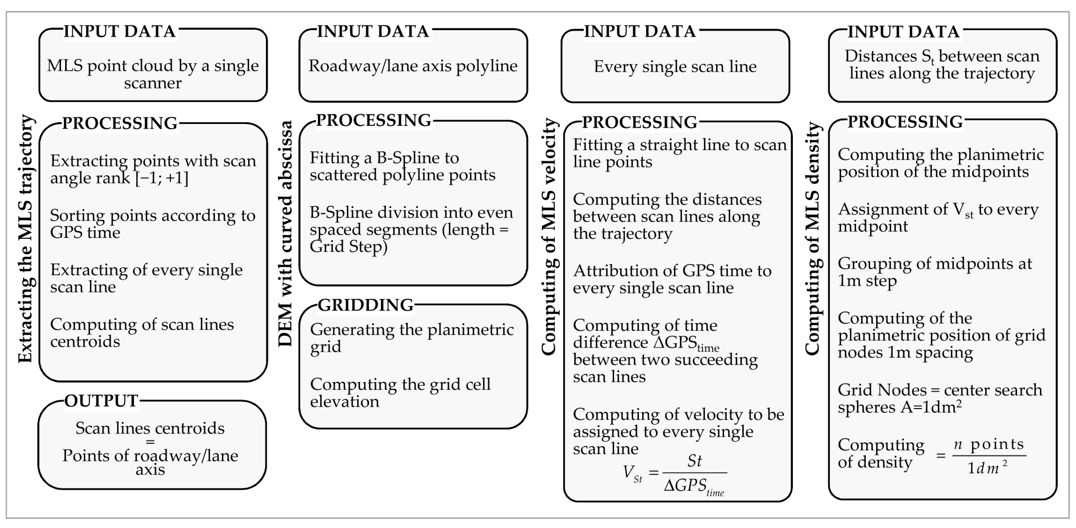
The spatial resolution of the DEM is one of the most important parameters characterizing it. Since it is dependent on the density of the acquired MLS data, we also describe the method developed for the computation of the point cloud density and of the distance between scan lines, as the MLS travel velocity varies. The DEM resolution should be set not only in accordance with the spatial distribution of the data (density) but also with the type of distress to be investigated. Hence, in the design phase of the survey, it is advisable to consider the types of distress to be monitored, which will mainly determine the velocity of the vehicle instrumented with the MLS. Figure 1 shows the schematic of data processing. The input data consist of point clouds coming from the two scanners assembled in the MLS system. The whole process was implemented in MATLAB.

The main processing steps are as follows:

• Extraction of all scan lines one by one from the MLS point cloud acquired by a single laser scanner. The centroids of each scan line will be the vertices of a polyline that outlines the trajectory;
• Computation of the spacing between consecutive scan lines, both the distance (S_LD) between them and the distance (S_t) along the trajectory. Along this direction, the “instantaneous” velocity (V_St) is also estimated;
• Computation of the density, estimated as number of points/dm². The density values are computed around the nodes of a 1 m × 1 m grid, which are placed along the MLS trajectory and orthogonally to it, in both directions (right and left), up to 6 m away. The average velocity (V_G) will be related to the density.
• Construction of a DEM with curved abscissa. The abscissa polyline is made up of the points corresponding to the axis of the road/lane given as input.

2.1. Computing of Travel Velocity

Before continuing with the processing of the data derived from the MLS survey, the point cloud should be edited since it is made up of the points that shape all of the elements on the road scene; they can either belong to the road surface (GP, ground points) or not belong to it (NGP, no ground points). The extraction of the bare road surface (made of GPs only) and the removal of the outliers was carried out by applying the method introduced in [37]. The procedure is based on the MSAC (M-estimator Sample Consensus) method.

GNSS receivers mounted on MLS usually acquire positioning data at frequencies ranging from 1 to 10 Hz, some are able to acquire data up to 20 Hz. Accordingly, the highest-performing receivers will be able to acquire the coordinates of a point every 1.4 m or so, down to 0.7 m for those at 20 Hz.

The IMU provides orientation data at a frequency from 100 to 2000 Hz and, combined with the DMI, integrates GNSS data in order to improve the computation of the trajectory, also in terms of linear resolution. These data are not always released and included in the output file containing the data sourced from the laser system.

Therefore, the method of computing the velocity of the mobile vehicle that we developed disregards the raw data but directly deals with the point cloud being the output of the MLS, in order to make the method more general and not dependent on the inertial platform data.

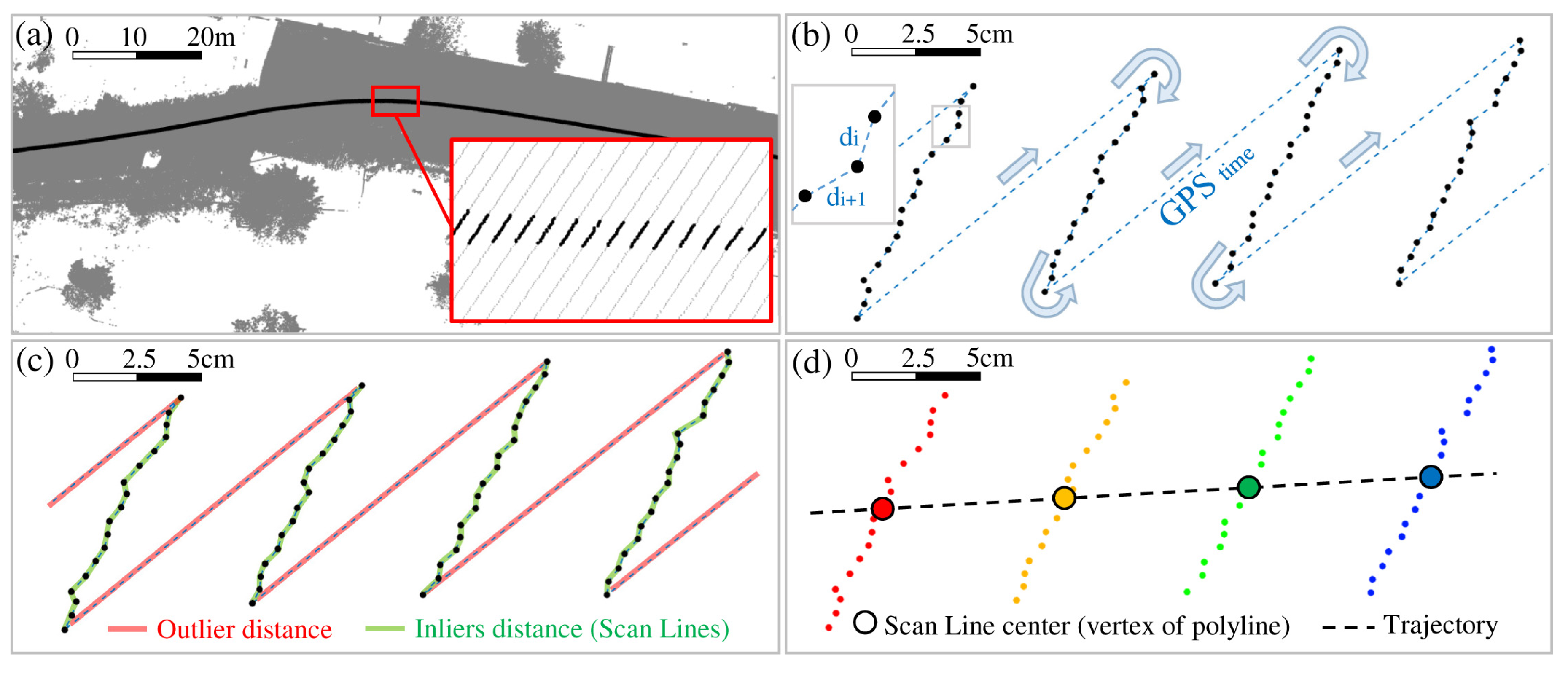
The first step of the elaboration process starts with extracting from the edited point cloud only those points corresponding to the trajectory. From the point cloud produced by a single scanner, given as the input, only the points with scan angles (sexagesimal degrees) in the range [−1, +1] were extracted (Figure 2a). Next, these points were sorted in ascending order according to GPS time and the Euclidean distance between the pairs of points, so sorted was computed (Figure 2b). Then, to extract and isolate the individual scan lines, a search for outliers was run on the array containing the values of the distances (point to point, Figure 2b); a distance value 3 times greater than the median absolute deviations (MAD) is referred to as an outlier (Figure 2c). The centroids of each extracted scan line are the vertices of the trajectory polyline (Figure 2d).

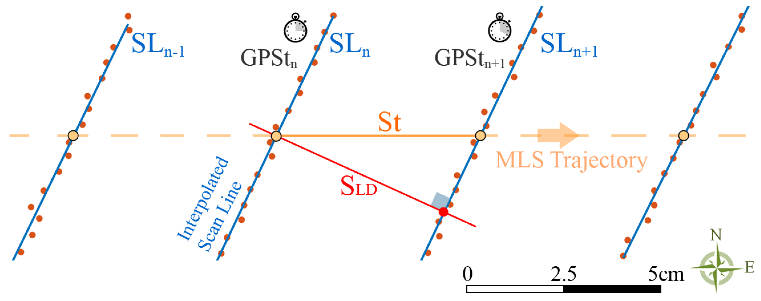
Along the trajectory, the MLS travel velocity (V_St) is computed for each pair of scan lines (SL, Figure 3).

Given the GPS time (GPS_t) associated with each scan line, the difference between the times of two successive scans is given by:

$$\Delta GP{S}_t=GP{S}_{t(n+1)}-GP{S}_{t(n)}$$

(1)

Velocities are computed as follows:

$$V_{St}(S{L}_n,S{L}_{n+1})=\frac{St}{\Delta GP{S}_t}$$

(2)

$$S_{LD}=d(S{L}_n,S{L}_{n+1})$$

(3)

where S_t is the Euclidean distance between two scan lines at the intersection points with the trajectory and the S_LD is the distance between the two least-squares interpolated straight lines representative of the scan lines. The coordinates of the intersection points were computed using the “polyxpoly” function. Figure 3 shows a zoomed-in view of scan lines with scan angles in the range [−1; +1]. The smallest GPS time value of all the points of the scan line is assumed as the GPS time associated with the n-th scan line (SL_n).

2.2. Computing of Density

Density is a critical parameter in the choice of the DEM step, which must be taken into account during the design phase of the MLS survey since it is related to the velocity of the moving vehicle.

Density computation implies the computation of the number of laser points contained within a certain area, in our case the area of a circle equal to 1 dm². The densities were computed at the nodes of a 1 m × 1 m grid. The point clouds acquired by both lasers of the MLS are being considered.

The procedure implemented to find the coordinates of the grid involves the following steps:

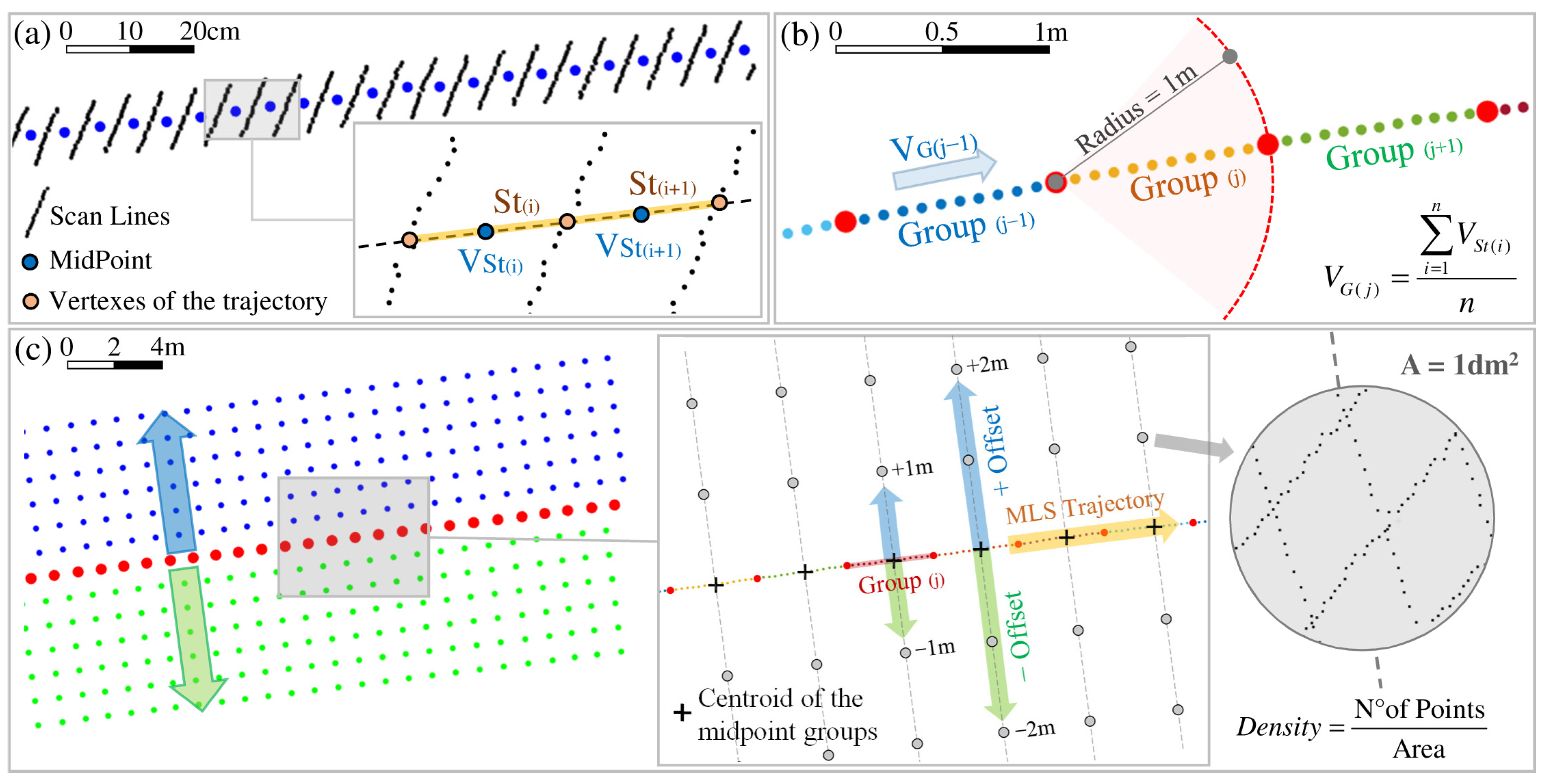
• Computation of the planimetric coordinates of the midpoints of the segments S_t (Figure 4a). To each midpoint the velocity V_St is assigned (Equation (2) in Section 2.1);
• Grouping of midpoints at 1 m intervals along the trajectory by using the “findNeighborsInRadius” function (Figure 4b);
• Computation of the planimetric coordinates of both the centroid of the midpoint groups and the nodes of a grid placed at given offsets d from the centroids, ranging from 1–6 m in steps of 1 m, in the direction orthogonal to the trajectory, from both sides (Figure 4c).

The density is estimated as the number of points contained in search spheres whose radius r is set so that their area is equal to 1 dm² (r sphere ≈ 0.564 dm). The centroids of the midpoint groups and the “offset points” (grid nodes) are the centers of the search spheres. To all the points of a group, inside the sphere of circumference 1dm², is associated an average velocity V_G computed as follows:

$$V_{G(j)}=\frac{{\displaystyle \sum _{i=1}^n{V}_{St(i)}}}{n}$$

(4)

where j indicates the j-th group and i the i-th point of the n points belonging to the group (j).

2.3. Construction of DEM with Curved Abscissa

The DEM that we aim to build consists of a grid model of the road surface with curved abscissa corresponding to the axis of the roadway/lane. It is represented as a raster matrix $D\in {ℝ}^{n,c}$ that contains the elevation value, derived from the interpolation of each node of the grid. The matrix contains n rows, equal to the number of vertices of the axis polyline and a number of columns c equal to the number of nodes comprising the generic cross section. The vertices of the polyline $S_o\in {ℝ}^{n,2}$ belong to the road axis.

2.3.1. Axis Polyline Construction

The algorithm asks for a polyline as an input representing the roadway axis or the lane axis (it depends if you are modeling the roadway or a single lane).

The polyline can be either in vector format or in ASCII format, i.e., a text file containing the coordinates of the vertices, as it is for the GNSS measurements.

The coordinates of the P_i vertices belonging to the polyline that defines the axis of the roadway or individual lane $P\in {ℝ}^{np,2}$ could be derived from a variety of sources, including for example:

• GNSS tracking of the horizontal signage of the roadway axis [38];
• Horizontal signage extraction from point cloud and roadway axis vectorization [39];
• Extraction of MLS trajectory [37], in the case of a single-lane analysis and only if the vehicle has traveled along the section under consideration without performing evasive maneuvers (e.g., overtaking) or other types of maneuvers that compromise the condition of parallelism between MLS trajectory.

In all cases, the way that the axis polyline is made does not allow for the curved path of the road to be taken into account since it is discretized by segments of varying length, depending on the method used to obtain it. Thus, the polyline must be converted into a B-spline, which is a regular curve that represents a continuous mathematical function. The B-splines are generalizations of Bezièr curves, which allow for the construction of a smooth curve that passes through a number of control points by coupling several Bèzier curves, so as to obtain any possible curved path [40]. There are many different types of B-splines; in particular, we choose the cubic B-spline, which is most suitable for the modeling of road axes [41,42]. In our case, the B-spline curve is built using the P_i vertices of the input polyline as control points.

Given the np control points (the vertices P_i of the input polyline) belonging to the matrix, the function B-spline B_s is defined as follows:

$$B_s(t)={\displaystyle \sum _{i=0}^{np}{B}_{i,h}(t)P_i}$$

(5)

where h is the degree of the polynomial, and B_i,h are the polynomials computed with de Boor’s formulas [43].

For the generation of the polynomial B-spline curve, the function “bsplinepolytraj” was used; the function generates a piecewise cubic B-spline trajectory starting from the control points (the control points are the vertices of the input polyline belonging to the matrix). The output is a matrix containing the planimetric coordinates of the B_si vertices of the cubic B-spline trajectory. In addition to the control points, the function requires a sample parameter as an input to transform the interpolated continuous polynomial functions into a discrete one. The number of vertices nv of the output function is driven by the value given to the sample parameter, which in turn is related to the grid step. Figure 5 shows an example of cubic B-spline generation (red line) from the input control points (blue crosses); the black dots show the discretized B-spline.

The next step consists of dividing the B-spline curve into straight segments of constant length, equal to the longitudinal step ρ_l of the DEM grid.

The algorithm is based on an iterative process and follows the main steps:

• Starting from the first vertex of the B-spline, a circle of radius equal to the step ρ_l is built. The planimetric coordinates (E_c, N_c) of the points lying on the circumference are computed with the equations:

  $$\begin{array}{l}{\alpha }_{\pi }=\left[0:\frac{\pi }{k}:2\pi \right]\mathrm{with}k>200\\ E_C=E_{Bs1}+{\rho }_l\cdot \cos ({\alpha }_{\pi })\\ N_C=N_{Bs1}+{\rho }_l\cdot \sin ({\alpha }_{\pi })\end{array}$$

  (6)

  where E_Bs1 and N_Bs1 are the planimetric coordinates of the first vertex of the B-spline.
  The coefficient k is a scalar that defines the degree of discretization by points of the shape of the circumference: the greater the circumference, the greater the number of points that describe it. Based on our tests, values of k > 200 allow the circumference to be discretized with points regularly spaced at the selected distance.
• To compute the coordinates of the intersection points of the circumference with the B-spline curve, the “polyxpoly” function is used. It should be noted that the function generates vector polylines, i.e., joins the vertices given as inputd with line segments, this means that a more resolved discretization for both geometric entities leads to better results (as described above with regard to the k-scalar).
• The process is run again. The new circumference is generated as in step 1, except that the coordinates of its center are replaced by the planimetric coordinates of the point previously determined via the intersection.
• The process ends when the intersection function returns empty vectors. It should be noted that, from the second computation onwards, the algorithm will compute a pair of points by means of intersection; the point chosen will be the one that follows the direction of travel of the B-spline (generally associated with GPS time). The planimetric coordinates of the n vertices of the B-spline at constant spacing will be contained in the matrix $S_o\in {ℝ}^{n,2}$.

2.3.2. Generating the Planimetric Grid

The next step is to build the planimetric grid of DEM nodes starting from the regularly interspaced vertices of the B-spline.

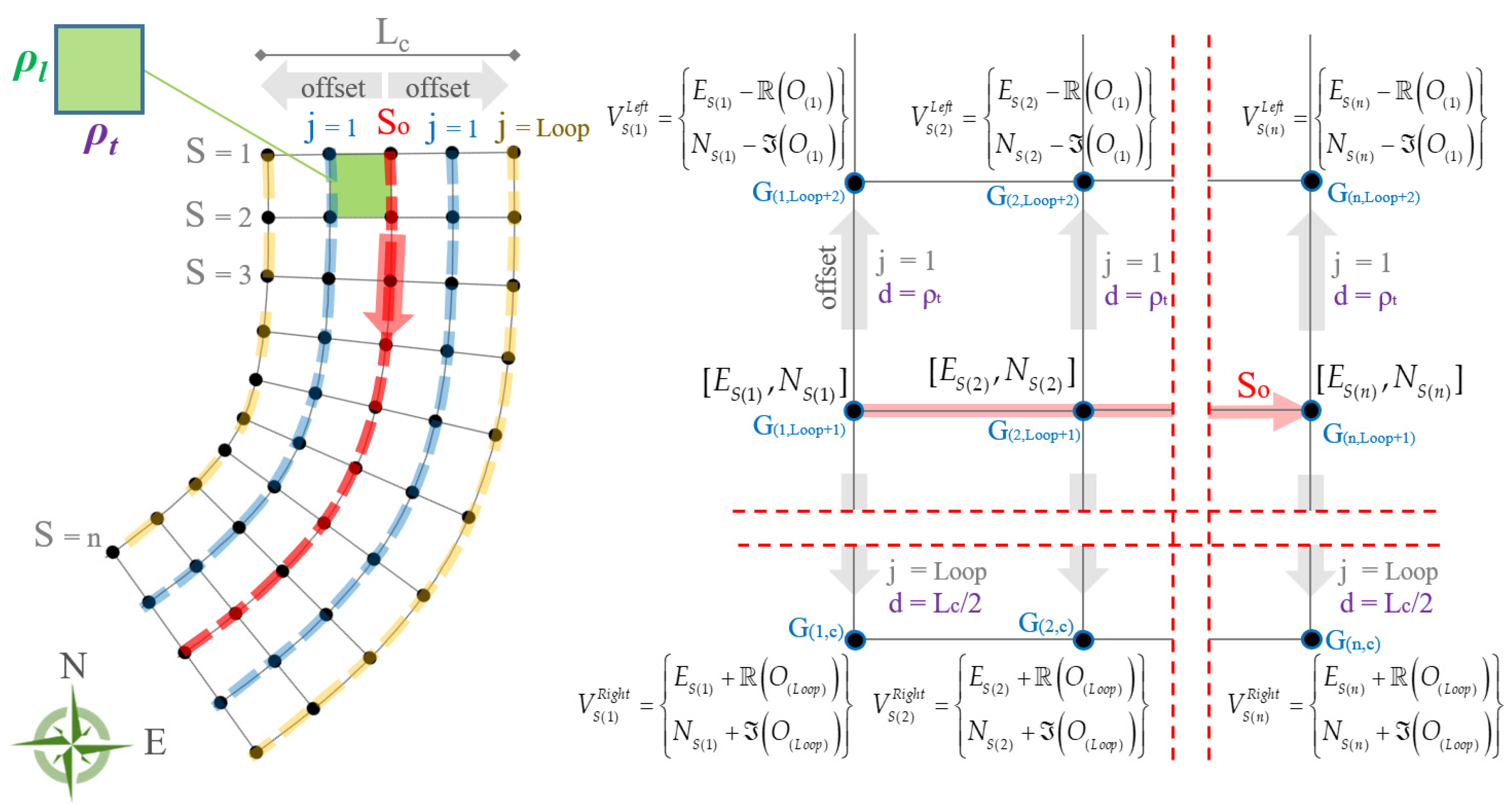
The whole process is iterative; at each iteration, an offset (at constant cross-spacing ρ_t) is computed from the axis vertices belonging to the matrix S₀. The total number of iterations “Loop” is a function of the roadway width (L_c) and the cross axis spacing ρ_t:

$$Loop=\frac{\left(\frac{L_c}{2}\right)}{{\rho }_t}$$

(7)

The command that implements the algorithm to compute the generic offset (j-th, with j going from 1 to Loop) works as follows:

• Given the n vertices S of the B-spline placed at constant spacing ρ_l, whose planimetric coordinates are contained in the matrix $S_o\in {ℝ}^{n,2}$, a row vector $M\in {ℂ}^{1,n}$ containing the following complex function is built to compute the coordinates of the offset points:

  $$M_{(j)}=E_S+im\cdot N_S$$

  (8)

  where E_S and N_S are the coordinates of the vertices S belonging to the polyline and im is the imaginary unit (im = 0.0 + 1.0·i).
• Next, the row vector $\Delta M\in {ℂ}^{1,n-1}$, which contains the coordinate differences between the S_th vertex and the S_th−1, is built:

  $$\Delta M_{(j)}=\left[\left(E_{S+1}+im\cdot N_{S+1}\right)-\left(E_S+im\cdot N_S\right)\right]$$

  (9)
• Next up, the row vector $\Delta M^{II}\in {ℂ}^{1,n}$ is built:

  $$\Delta M_{(j)}^{II}=\left[\Delta M_1,\frac{\left(\Delta M_{1:n-2}+\Delta M_{2:n-1}\right)}{2},\Delta M_{n-1}\right]$$

  (10)

  where $\Delta M_1$ indicates the first element of $\Delta M$, $\Delta M_{1:n-2}$ indicates the elements of from the 1_st to the n_th-2 (with n = number of vertices) and $\Delta M_{n-1}$ indicates the last element of the row vector $\Delta M$, which has the dimensions (n − 1).

For each pair of planimetric coordinates E_S, N_S of the generic vertex S, the two pairs of offset coordinates $E_o\in {ℝ}^{1,2},N_o\in {ℝ}^{1,2}$ are obtained by subtracting and adding the scalar of the real or imaginary part of the respective row of the matrix $O\in {ℝ}^{1,n}$. The formulas are:

$$\begin{array}{l}{E}_{o(j)}=\left[E_S-ℝ\left(O_S\right),E_S+ℝ\left(O_S\right)\right]\\ N_{o(j)}=\left[N_S-\Im \left(O_S\right),N_S+\Im \left(O_S\right)\right]\end{array}$$

(11)

The terms of the row vector $O\in {ℂ}^{1,n}$ are:

$$O_{(j)}=\frac{d\cdot \Delta M_{(j)}^{II}\cdot e^{-im\cdot \frac{\pi }{2}}}{\left|\Delta M_{(j)}^{II}\right|}$$

(12)

In the first iteration, the value of the offset d is equal to the value of the cross step ρ_t that is selected. In the subsequent iterations, the offset value d is increased by ρ_t:

$$d=d+{\rho }_t$$

(13)

Figure 6 shows a schematic drawing of the offset process for generating the planimetric curvilinear grid.

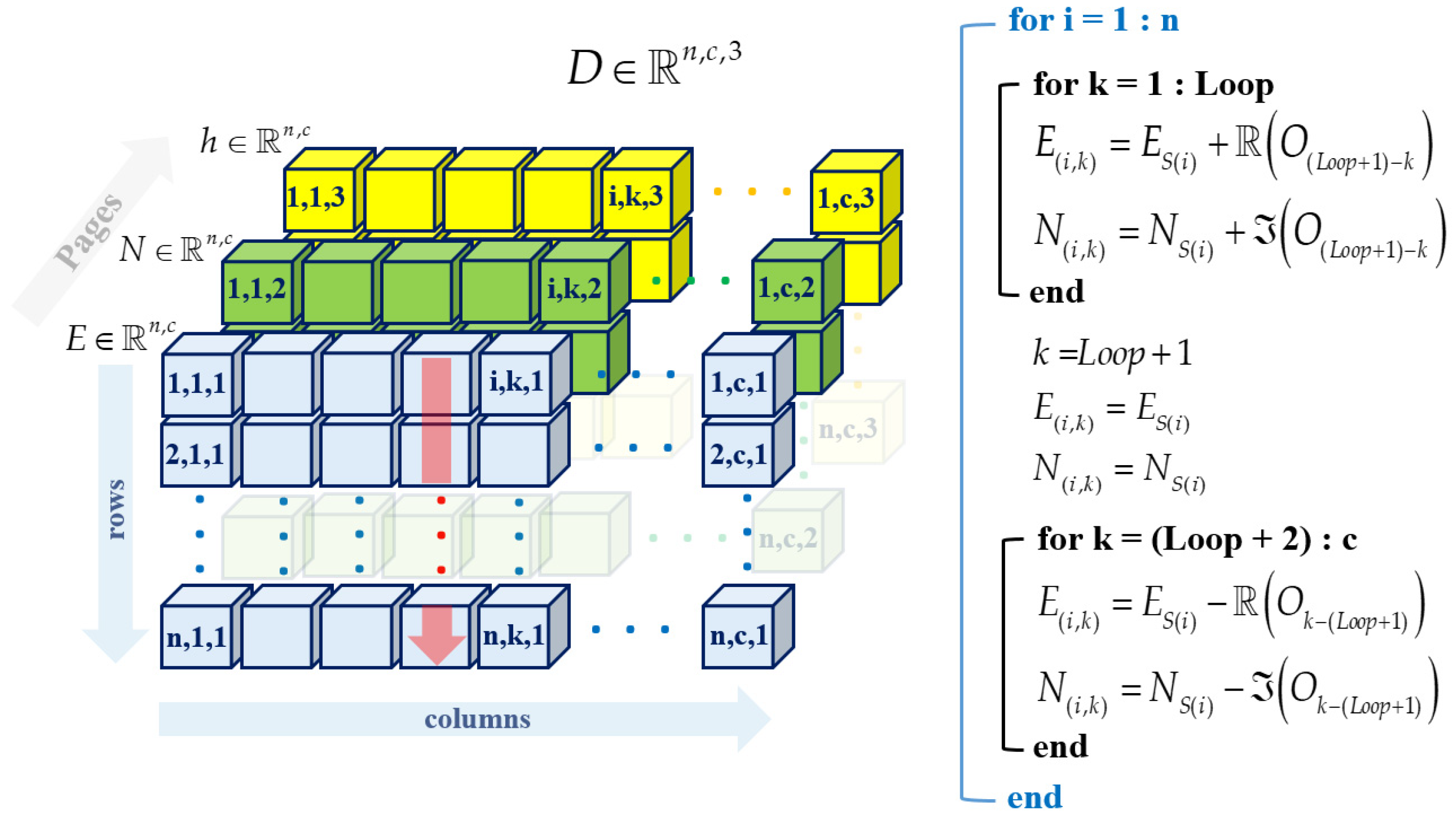
The planimetric coordinates of the nodes are contained in a 3D array $D\in {ℝ}^{n,c,3}$, characterized by three overlapping 2D arrays with n rows (n equal to the total number of vertices S) and c columns $c=\left(2\cdot Loop\right)+1$. The third dimension is formed by pages or sheets (in our case equal to 3), which allow the desired level to be selected (Figure 7).

The planimetric coordinates of the grid nodes are contained in the first two levels (page 1 and page 2), the east coordinates $E\in {ℝ}^{n,c}$ in page 1 and the north $N\in {ℝ}^{n,c}$ in page 2. The node elevation values $h\in {ℝ}^{n,c}$ will be contained in page 3.

Naming with k, the k-th column of the arrays E and N, with the i the i-th rows, the planimetric coordinates of the nodes, computed by running the offset algorithm, are ordered in the corresponding array as shown in Figure 7.

Each row of the matrix $D\in {ℝ}^{n,c}$ represents the cross section orthogonal to the axis polyline at a given progressive, whereas the columns represent the longitudinal profiles.

From here on, we refer to this new DEM with curved abscissa as DEMc.

2.3.3. DEMc Resolution

The DEM resolution that is determined by grid spacing should be dependent on the point density. For a homogeneous distribution of points, to estimate the proper value for grid spacing ρ, the following formula may be used [34]:

$$\rho =0.5\sqrt{\frac{A}{N}}$$

(14)

where A is the area of the analyzed road surface in dm² and N is the total number of points in the area.

The DEMc grid step chosen is set along the axis polyline; in the curved stretches of road it will undergo a variation, in particular, the convex part the step will undergo an increase, whereas in correspondence with the concave stretches the step will undergo a decrease. The minimum grid step in the concave areas, however, must be in accordance with the density of the point cloud.

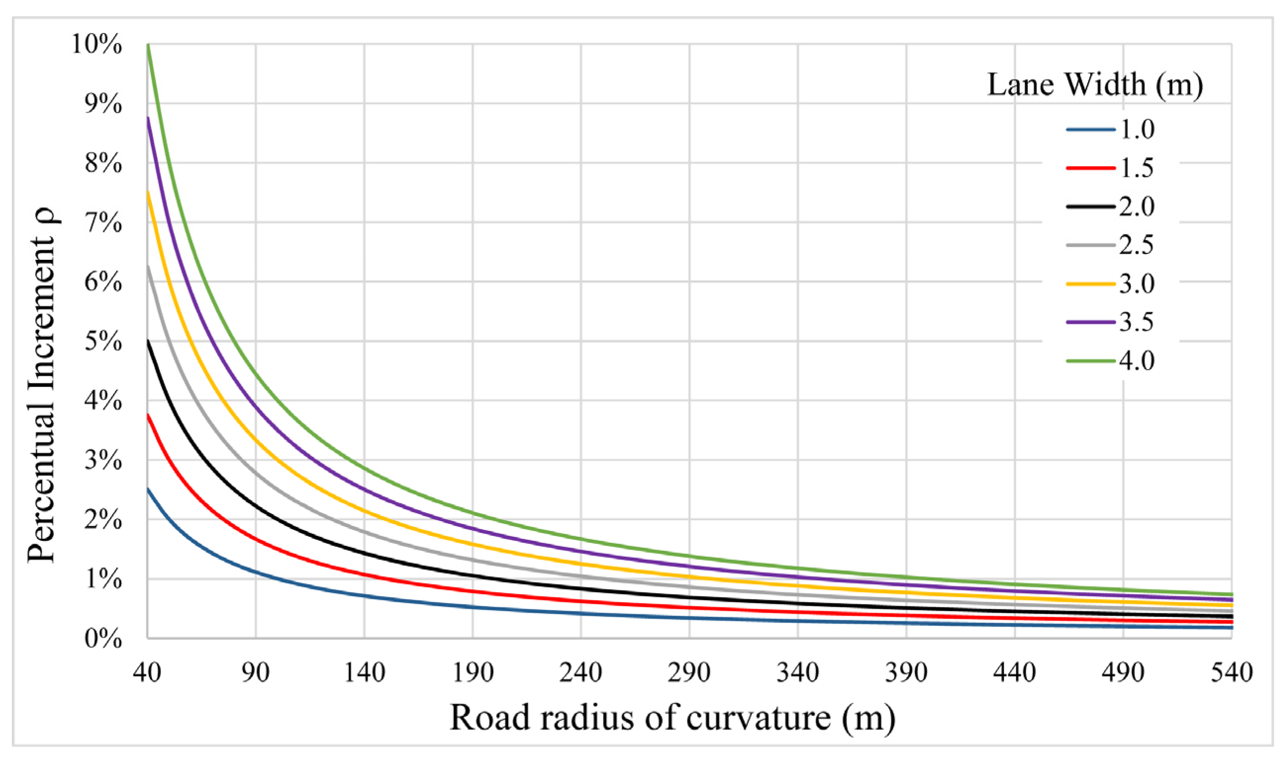
The graph in Figure 8 shows the increase in grid spacing and percentage value, as the radius of the circular curve and the width of the lane (from 1 to 4 m) vary. Only the trends of the percentages of increase (convex area) are shown, since the decreases are equal and of the opposite sign. As far as the radii of curvature are concerned, we only considered values up to 540 m because the percentage increases are not significant, as they are lower than 1% (less than a millimeter for a grid spacing of 10 cm).

The simplified equation for computing the percentage increase in grid spacing is as follows:

$$PercentageIncrease=\left(\frac{\left|{\rho }_{(Max,Min)}-\rho \right|}{\rho }\right)\cdot 100;{\rho }_{(Max,Min)}=\rho \cdot \left(1\pm \frac{Lw}{R}\right)$$

(15)

where L_w is the lane width, ρ is the grid step along the road axis and R is the radius of the circular curve.

2.3.4. Computing the Elevation of DEMc Nodes

The height values h of each single node are computed using spatial interpolation methods.

The process implemented is composed of two steps, with the aim of reducing the computational cost, given the large amount of data to be processed.

The first step of processing consists of subsampling the whole edited point cloud, henceforth referred to as PC, according to the following steps:

• The PC dataset undergoes a 3D grid subsampling process, using the “gridAverage” function. To specify the 3D cell size, a value for the “gridStep” must be set that is assumed proportional to the resolution of the planimetric grid:

  $$GridStep=\frac{\left(\frac{{\rho }_l+{\rho }_t}{2}\right)}{3}$$

  (16)
• The result is a point cloud $P{C}_d\in {ℝ}^{p,3}$ (with p = total number of points) subsampled and organized according to a cell diagram.
• The PC_d data are projected onto a horizontal plane at zero elevation by multiplying the vector containing the elevation values by 0; this results in the matrix $P{C}_{d0}\in {ℝ}^{p,3}$
• In Page 3 ($h\in {ℝ}^{n,c}$) the initial value is set to zero.

The second step consists of running a cycle of commands equal in number to the total number of nodes in the planimetric grid (for each element of the matrix $D\in {ℝ}^{n,c}$):

• For each node, the Np neighboring points (Np is given as input, by default Np = 6) belonging to the PC_d0 data are computed by running the “findNearestNeighbors” function, which outputs the row indices of the matrix PC_d0 corresponding to the Np points with the smallest Euclidean distance from the node.
• The elevations of the points of the cloud PC_d are selected by means of the indices, and the average elevation is computed to obtain an approximate value $h_{(i,k)}^{approx}$ of the node height.
• This approximate value of the elevation is needed to apply the function “findNeighborsInRadius” in the node. The function selects the points of the PC cloud contained in a sphere of radius equal to the KernelSize (input value, function of the grid step and density of the input data) with a center in the node itself $D_{(i,k)}=\left[E_{(i,k)};N_{(i,k)};h_{(i,k)}^{approx}\right]$.
• The interpolation process is applied using the points contained in the search sphere so as to compute the interpolated value of the node elevation h_(i,k). The search sphere will select all points in the original non-subsampled cloud.
• Page 3 is updated with the elevation values computed as above.

Five basic interpolation algorithms were implemented: moving average; inverse distance weighted (IDW) for different power values, ordinary kriging (OK), average and polynomial functions. Here, we used the IDW algorithm, since for very high-resolution DEMs such as those built to characterize the road surface, and given the high density of the processed point clouds, more robust algorithms do not give better results. The results of tests reported in a recent paper [6] showed that, for a 10 cm grid step, the differences between the elevations of the DEM built by interpolation with IDW and those obtained using Kriging were smaller than the accuracy of the method itself and, therefore, not significant.

3. Test Case

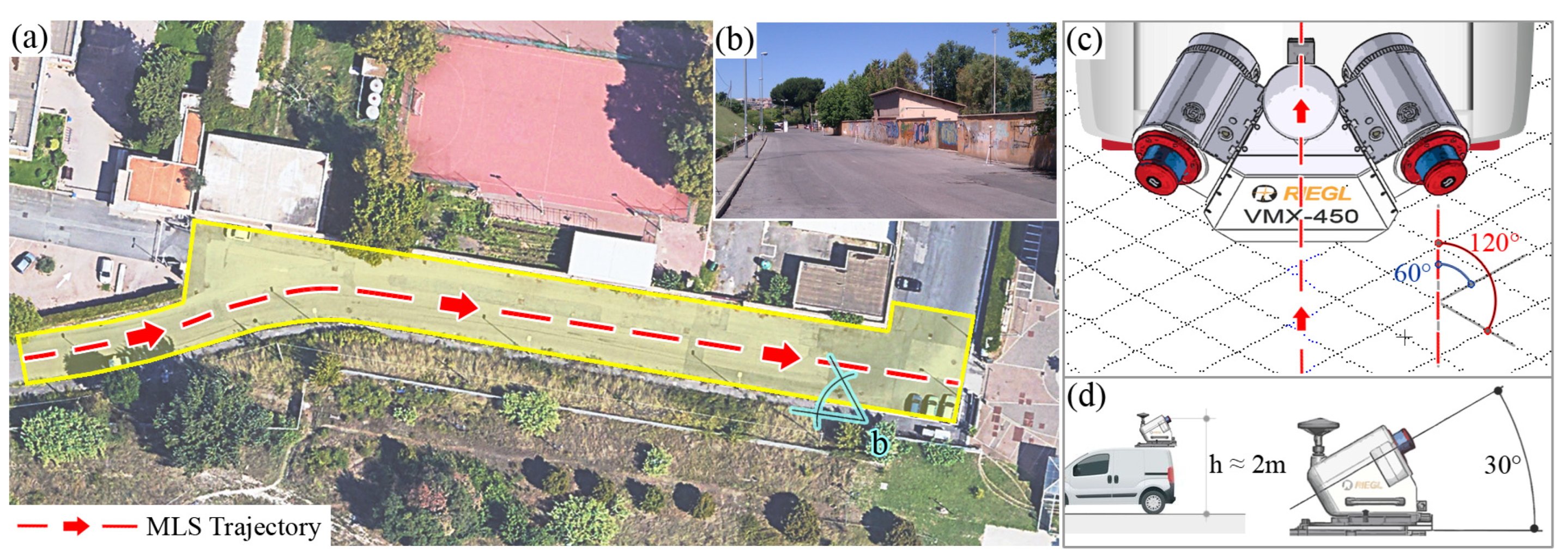
The test area is located in the municipality of Rome and consists of a road section that extends for about 150 m (Figure 9a,b). The section is made up of a single carriageway about 11 m wide with a double lane; each lane is about 3.5 m wide, the remaining space on the sides is reserved for parking. On one side, there is a sidewalk, on the other side a high wall with some access gates. The presence of different types of distress (cracks, potholes, swells, shoves, depressions) and the cross-sectional width of the carriageway make it suitable for validation purposes.

The survey was carried out with an MLS Riegl VMX-450 mounted on the roof of a car. The system was equipped with inertial and GNSS sensors and housed under an aerodynamic protection dome, in order to perform moving scans and georeference these scans to an external reference system. The unit consists of two Riegl vQ-450 laser scanners inclined at 30°, each with a 360° field of view (butterfly arrangement) (Figure 9c,d).

The trajectory is provided by the post-processing computation of kinematic differential GNSS measurements acquired with a dual-frequency geodetic receiver. The result is a point cloud, georeferenced according to the reference system UTM/RDN2008. A metadata file, as described in the American Society for Photogrammetry and Remote Sensing (ASPRS) specifications, is associated with the point cloud [44]. Among these the most common data are: (i) the amount of the reflected power (energy intensity); (ii) the return number; (iii) the GPS time (the double floating point time tag value) of the laser pulse; (iv) the angle scan rank (the angle between the zero reference and the direction of the laser beam, rounded up to the nearest integer in absolute value).

MLS acquires data by scan line. The spatial configuration of the scan lines depends on the system setup parameters, i.e., vehicle velocity, orientation of the scanners with respect to each other and with respect to the ground and rotation rate.

The vehicle traveled twelve times on that stretch of road at different average velocities (MLS_V): 10, 20, 40, 60 km/hour, with a constant sampling frequency (550 kHz). The MLS used, in addition to the frequency, requires as input data the average travel velocity that is planned to be maintained during the survey (Velocity Set “V_SET”). Given the same average velocity of the MLS, a different V_SET value was set (10, 20, 60 km/h) to evaluate its incidence in the various configurations. The maximum obtained point density value ranges from 3000 points/m² for average velocities of 60 km/h up to 35,000 points/m² for average velocities of 10 km/h. The minimum density on the roadway is about 500 points/m².

4. Results and Discussion

The tests carried out and the data processing methodology developed allow the relationship between the input parameters of the survey (scanning frequency, velocity setting) to be quantified with the density of the points acquired, the resolution of the DEMc, and lastly, with the type of distress that can be identified.

The density of points in the cloud is dependent on the actual travel velocity, yet the rotating laser that is part of the system outputs points at variable spacing in the cross direction (greater for more distant points and more evenly distributed in the travel direction and as a function of actual travel velocity).

Figure 10 shows for each velocity an excerpt of the density map represented through a chromatic scale that shows how the density to the path is almost longitudinally constant, while it ranges greatly with the velocity (from 30,000 points per m² to 3000 when the velocity increases from 10 to 60 km/h), while crossways, the variation is very fast even for the few meters of the roadway width (at the roadsides it decreases to 3000 pts/m² for a velocity of 10 km/h and to 500 pts/m² at 60 km/h).

Given the strong correlation between density and the actual velocity that was estimated, as described in Section 2.2 (Equation (4)), we aimed to derive a functional relationship between the experimental data that also accounted for the distance from the trajectory in the cross direction; longitudinal stripes were considered for distances (d) from 1 to 6 m.

The MLS used allows the input of the average velocity value (velocity set parameter, V_SET); the set value also affects the rotation speed of the scanner, i.e., the number of lines per second recorded. To study the effect of this parameter, V_SET values equal to 10, 20, 60 km/h were set, while maintaining different effective travel velocities to analyze the data acquired in a variety of scenarios. Multiple passages were driven at different actual average velocities, 10, 20, 40, 60 km/h.

Figure 11 shows the diagrams of the density as a function of the velocity V_G. The diagrams shown in panels a,b,c refer to the V_SET settings of 10, 20 and 60 km/h, respectively.

The coefficients of the equation that defines the best-fit exponential curve for the density data were found using the least squares method. The different color is to specify the distance from the trajectory (from 1 to 6 m). The coefficient values are reported in panel d as well as the value of the coefficient of determination R², which defines how well the model fits the data.

The data graphed in the figure show that the vehicle is not always capable of traveling at a constant velocity; therefore, the density values, while more centered on the design values, are somewhat scattered, especially when traveling at low velocities.

From the comparison of the curves plotted in the three panels of the figure, it should be noted that the use of different V_SET values does not result in a significant change in the best-fit curves, whose trend depends almost only on the actual velocity V_G; the R² values also remain very similar.

The exponential curve fits the experimental data well, especially near the strips at distances less than or equal to 3 m, with R²~0.98, whereas for greater distances, the coefficient of determination decreases rapidly. This is probably due to the increased angle of incidence between the laser beam and the pavement, which results in greater areas of shadow (mainly in areas where the pavement is more distressed), and thus there is a non-uniform density of the data. Additionally, a big difference between the values of V_SET and V_G results in a decrease in R² for great values of d.

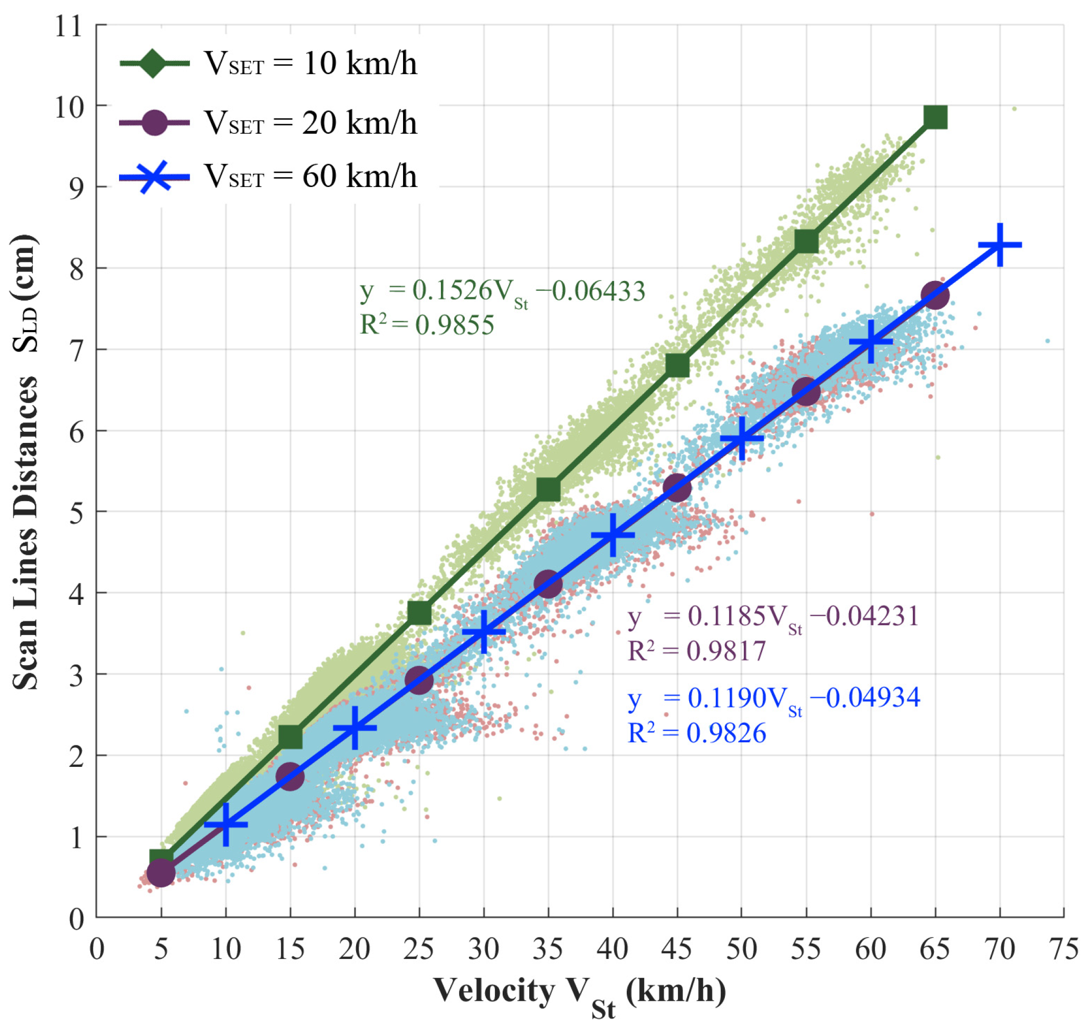
To better analyze the effect of V_SET, the relationship between the velocity V_St computed for each pair of consecutive scan lines (Equation (2)), and the distance S_LD between them, was also computed for the three different V_SET values. The correlation is linear, as Figure 12 shows. The point clouds are overlaid with the corresponding linear regression line; the coefficients of the equations and the coefficients of determination R² are also shown in the figure.

The diagrams show that the velocity V_SET being set in the system appears to affect the laser frequency only below a predefined set velocity (10 km/h), since the clouds relative to the other velocities appear as nearly overlapping, and the corresponding regression lines have almost equal coefficients, so that, for V_SET set at 20 km/h or 60 km/h, there is the same increment in the S_LD inter-distance as V_St increases.

The slope of the best-fit line for V_SET = 10 km/h is sharper than for the others; therefore, the distance between scan lines increases more rapidly than when V_SET is greater than 10 km/h.

It follows that, for computing the DEM grid spacing, it is advisable to choose the equation in which the grid step is a function of density (Equation (14)).

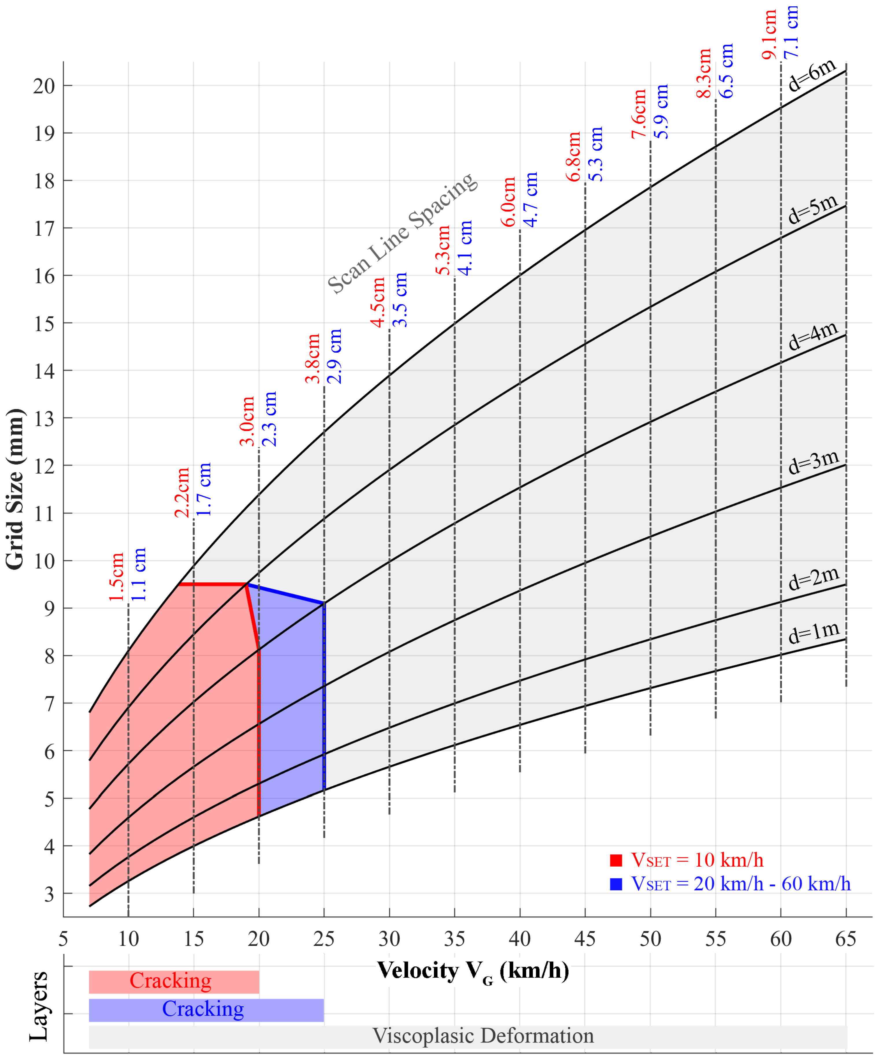
By using Equation (14), the grid spacing was computed as a function of the density values derived from the experimental data. The density in turn is related to the velocity V_G. Figure 13 shows the plot of grid step as a function of velocity V_G at various distances d from the MLS trajectory. Additionally, shown on the diagram is the minimum scan line distance (S_LD) for the different velocities considered.

On the diagram, the domains of the quantifiable distress are highlighted; in particular, three different layers are identified, representative of three main macro-groups [24,45]: (i) the cracking according to the resolutions compatible with V_SET = 10 km/h, identified by the red area; (ii) the cracking according to the resolutions compatible with the V_SET > 10 km/h, identified by the blue area; and (iii) the viscoplastic deformation identified by the gray area.

The geometric parameters specific to these macro-groups, used to delineate the domains in Figure 13, were derived from the relevant literature [24,33].

The boundaries of the function domains of the distresses were identified following the criterion indicated in the Nyquist–Shannon sampling theorem, so as to avoid the phenomenon of aliasing. A two-dimensional road profile is theoretically represented by the continuous addition of different sinusoidal curves, each characterized by a different wavelength λ and amplitude h [46]. The pavement texture can be divided into different classes, each with different wavelengths and amplitude intervals. Each distress is then characterized by a particular combination of wavelength and amplitude, for example: cracking, belonging to the macro-texture class, having both wavelengths and amplitudes (0.5 < λ < 50 mm, 0.2 < h < 10 mm) that are significantly shorter than the viscoplastic deformation group (50 < λ < 500 mm, 1 < h < 50 mm), and belonging to the mega-texture class.

When discretizing the signal, the constant sampling interval should be set at no greater than half the wavelength of the sine wave representing the road profile. This is derived from the Nyquist–Shannon sampling theorem [47], which defines the minimum frequency required to sample an analog signal without the loss of information (aliasing). The resolution of the DEM consistent with the distresses should, therefore, be equal to their characteristic planimetric dimensions halved, so that there will be no loss of information.

In order to obtain lossless samples, it is advisable to use two points within the wavelength of the distresses being analyzed [47,48]; if cracking belongs to the macro-texture class (0.5 < λ < 50 mm), 25 mm should not be exceeded as the sampling interval. In the worst case scenario of using the distance between two scan lines as a reference (thus assuming that only one laser is used) and analyzing a single longitudinal profile, the scan lines should have inter-distances that do not exceed 25 mm, in order to discretize cracking with wavelengths of 50 mm. If two scanners are used, the pattern becomes square-meshed, and thus the distance between two scan lines may slightly exceed the 25 mm limit.

The results of the tests we conducted suggest that choosing 30 mm as a grid size is an appropriate choice. Consequently, driving velocities of 20 km/h (for V_SET set at 10 km/h) and 25 km/h (for V_SET at 20 or 60 km/h) should ensure a discretization of the generic profile without the loss of data, since the scanning lines are about 30 mm apart.

In order to detect cracking or other types of distress in the DEMc of the road pavement, a resolution of the laser data is required that allows for their correct discretization and modeling. Given the characteristics of the data in terms of resolution, the grid resolution should be chosen to be compatible with the data and allow a proper modeling of cracking or other distresses, that result in a more accurate quantification of the same distresses.

The limit value of grid size is also chosen to be compatible with the characteristic dimensions of the distress to be analyzed. Similarly, according to the Nyquist–Shannon sampling theorem, to obtain the correct modelling of cracking, and therefore a correct measurement of their extent, a grid size must be chosen that is at least equal to half the value of the extent of the dimensions, which is related to the studied severity level. In our tests, the thresholds chosen for the different types of distresses correspond to an average severity level. For cracks, the average severity levels correspond to 19 mm, in terms of crack width; therefore, the frontier was chosen at 9.5 mm.

To verify the effectiveness of the proposed method to be used for the design of the MLS survey, which aims to identify some specific type of distress, we analyzed a number of point clouds belonging to our dataset and verified whether the derived DEMc was able to identify and characterize the cracking status of the surface.

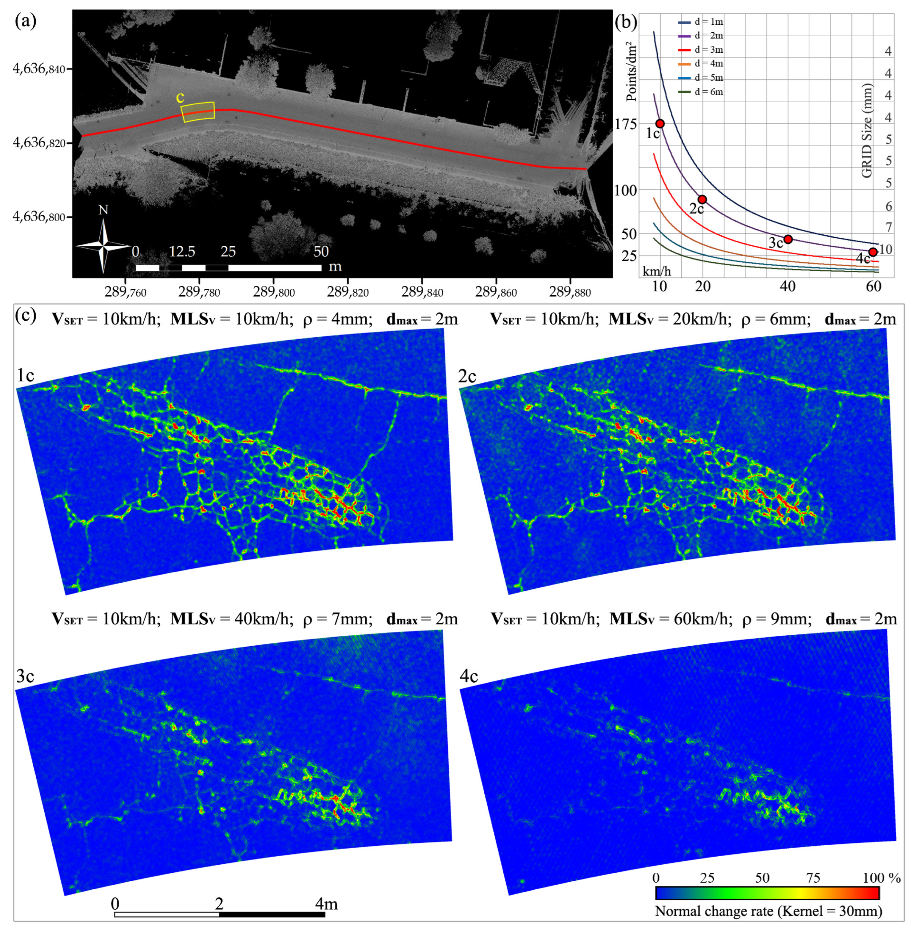
We analyzed a portion of road surface (Figure 14a, highlighted in yellow) 4 m wide, symmetrical to the trajectory followed by the MLS. For this section, we graphed the density as a function of travel speed V_G (Figure 14b) at various distances d from the trajectory keeping V_SET set to 10 km/h. On the curve corresponding to a 2 m distance from the trajectory (the second one from the top), we identified the velocities corresponding to certain densities (the four red circles 1c, 2c, 3c and 4c), which lead to grid sizes of 4, 6, 7 and 9 mm.

Once the grid size was chosen, the DEMc of the road surface was built by applying the method described in Section 2.3. In detail, to estimate the node elevation, the local interpolator IDW² was used, choosing a variable search radius for each direction depending on the distance between the scan lines.

Starting from the DEMc related to the height values, a DEM of derived features, which better highlight the monitored distresses is built; the parameter used to highlight the cracking status is the normal change rate, a simplified measure of the total curvature. To highlight the distresses, the local curvature variation, expressed as the normal change rate, was computed over a kernel size. The method implemented in CloudCompare software (https://www.danielgm.net/cc/ (accessed on 10 June 2021) was adopted.

In Figure 14, panel c shows the excerpts of the four DEMc built at different resolutions, related to the portion of the road highlighted with the yellow box in panel a.

In detail, the DEM in panel 1c provides evidence that the chosen resolution (4 mm) is suitable for the identification of the cracking present on the surface; characterized by medium/low levels of severity, the cracks are well distinguishable and free of noise. Panel 2c shows how the DEMc excerpt, built with data acquired by traveling with a MLS_V equal to 20km/h and thus a resolution of 6 mm, allows to distinguish the cracking status, but the cracks with low levels of severity are not visible and there is some noise, probably due to the resolution chosen in function of the density and therefore of the travel velocity that is that which corresponds to the frontier of the red domain (Figure 13).

Panel 3c shows the excerpt of the DEMc generated with data acquired by traveling with a MLS_V equal to 40 km/h, congruent with the resolutions in the field of viscoplastic deformations (Figure 13). It should be noted that the point cloud density and, accordingly, the minimum grid spacing do not allow for the detection of cracks with low/medium severity levels, as well as those acquired by traveling at a MLS_V of 10 km/h. Only those distresses congruent with the proper resolution are evident here, particularly some holes (red areas) and cracks with high severity levels, also present in panels 1c and 2c.

If the grid spacing is too large (thus outside the domain), the crack will, in a few cases, still be detectable but not quantifiable since it will appear as a deep groove proportional in width to the sampling interval (panel 3c). This will artificially increase the roughness of the adjacent area, due to the lack of information caused by the over-reduction in resolution.

Finally, panel 4c shows the DEMc relative to the data acquired by traveling with MLS_V = 60 km/h, with a resolution of 9 mm; in this case, the crack state is not detectable. The only clearly visible distresses are those belonging to the macro-group of viscoplastic deformations and some potholes produced by the removal of the surface layer of the pavement.

In summary, depending on the type of degradation to be investigated, the diagram can be used to estimate the travel velocity to be maintained and the maximum distance d from the MLS trajectory.

The diagram aims to help in the design phase, an essential phase prior to the survey, and to optimize the available resources. The resolution is a function of the type of analyzed distress, and the design travel velocity is computed accordingly. If the aim is to measure cracks up to a distance of 6 m from the MLS trajectory, a velocity of less than 15 km/h must be maintained.

In order to obtain an average grid step of 6 mm, a maximum driving velocity of about 35 km/h has to be maintained. More passages must be made to cover the whole road because the distance guarantees a resolution of about 1 m; therefore, in one passage, only 2 m is covered.

The maximum velocity that allows a DEM with a resolution of 10 mm to be built is 45 km/h up to a maximum distance of 3 m. To cover longer distances, with the same resolution value of 10 mm, the velocity must be reduced to 30 km/h to cover a distance of 4 m, to 20 km/h for a distance of 5 m, and to 15 km/h for a distance of 6 m.

Since the distances are computed with respect to the MLS trajectory projected onto the road surface, to analyze a single lane, the considered reference distance is about 2 m to the left and 2 m to the right of the trajectory (for a generic lane, 3.75 m wide), which provides an average resolution of 6 mm at an average velocity of about 25 km/h.

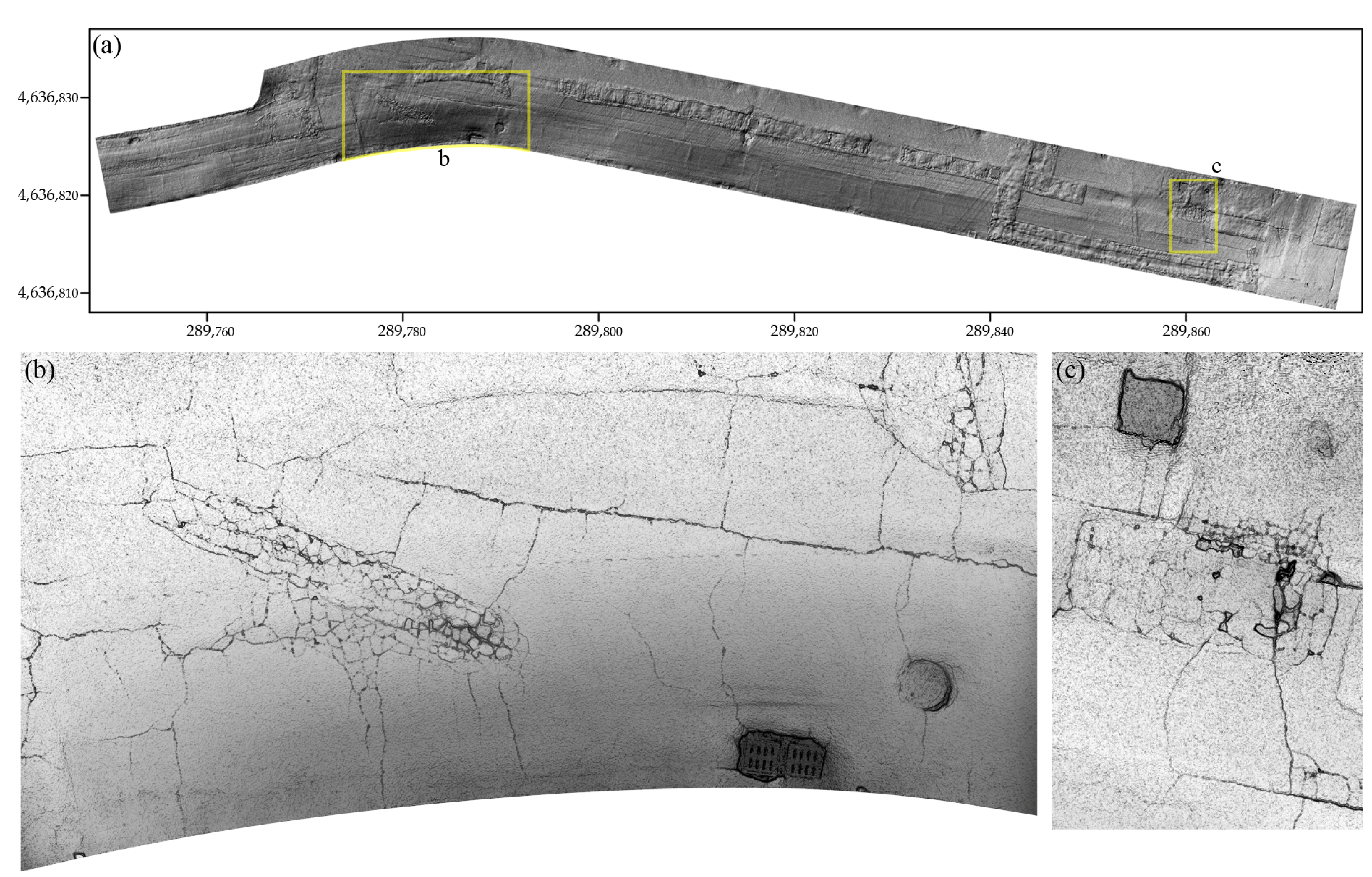
Figure 15 shows the DEMc built on the whole road stretch analyzed. The axis of the DEMc coincides with the axis of the roadway, the grid DEM has a semi-width of 5.50 m, so as to cover the whole 11 m wide roadway. The DEMc was built using the point cloud acquired by keeping the average velocity MLS_V equal to the V_SET one, at 10 km/h. This configuration, at 6 m distance, is compatible with a grid size of 8 mm (Figure 13). In correspondence to the curve section, in the concave inner part at 6 m from the roadway axis, we computed the decrease in the grid spacing with Equation (15). This was used to produce the graph in Figure 6, given the curve radius (about 45 m), which was equal to about 0.7 mm; hence, the grid spacing along the concave edge, in the longitudinal direction, assumed a value equal to 8.3 mm. We decided to set a conservative value for the grid spacing on the curved abscissa of the DEM, equal to 9 mm.

The data were interpolated using the IDW² interpolator. At the velocity of 10 km/h, the inter-distance between the scanning lines is about 1.5 cm. Given the configuration of the scanning pattern (Figure 9c), in the most unfavorable conditions where the generic node of the grid is in the center of the rhombus, the planimetric distance from the most distant vertex is equal to the inter-distance of the scanning lines. The search radius was therefore set equal to 1.5 cm.

The panels b and c of Figure 15 show two zoomed views of the DEMc, made in correspondence of areas characterized by different configurations and types of distresses. It should be that an accurate analysis of the grid size, in the functions of the main variables involved (density and travel velocity), is critical for optimizing the results, a key aspect during the design phase of a survey. Cracks with medium severity levels are clearly visible and can be quantified.

5. Conclusions

The knowledge of the surface pavement condition allows the extent of distress to be detected and estimated, so as to identify all those sections that need high priority interventions. The identification of the critical sections in a road network is mandatory in order to choose the most effective action and planning for the intervention program. A modern pavement management system should help in making decisions to ensure that safety and comfort are achieved at a minimum cost and that available resources are optimized. In most cases, however, planning operations do not aim to achieve an optimal process but tend to identify the best compromise between available budget and impending needs.

Although the MLS technique, in some cases, does not allow to reach accuracy and resolution as required by the managing authorities and by the current rules, nevertheless it allows a fast, at operating velocity, safe and economical survey of the pavement and of the boundary elements, ideal to draw up an emergency program of first intervention in a short time and at a very low cost.

The approach introduced in this paper focuses on three main aspects:

• The quantification of the relationship between the parameters given as input for the survey (frequency, velocity), and the density of the acquired points with the DEM resolution;
• The optimization of the process of extraction of profiles aiming to address the geometric characterization of the road;
• The optimization of the survey design by estimating the travel velocity to be maintained, and the maximum distance from the MLS that provides the expected resolution, related to the kind of distress to be investigated.

The proposed method aims to provide a contribution in the design phase of the survey, that is important for the optimization of available resources. The velocity held by the MLS during the survey is the key parameter for building a model to be used for distress identification.

The procedure described in this paper allows a simple relationship to be established that can be used to design an MLS survey for road condition monitoring. Given the density, it is possible to estimate the optimal resolution of the digital model of the surface compatible with it; the systematic tests carried out and the procedure developed made it possible to associate the velocity of the MLS with the resolution of the DEM, and therefore its capability to highlight distress at different levels of severity.

The resolution, therefore, will be a function of the kind of distress to be analyzed, and the velocity will be a function of the type of road to be monitored, in order not to compromise the normal exercise of the infrastructure.

The resolution is closely dependent on the relative accuracy of the MLS system used; in our case, it was very accurate and had a high performance. The MLS technique is actually in a phase of rapid development; the sensors are becoming better and more accurate and with ever better characteristics (e.g., ever higher frequency rates), and thus the accuracy and resolution are becoming better as well.

Moreover, the proposed methodology allows the operator to choose the most convenient strategy for monitoring the road network, the strategy that, given the same capability to highlight specific distress, maximizes productivity (shorter survey times and maximum velocity).

All of these issues were combined and quantified in the developed abacus (Figure 13). The grid step was chosen according to the kind of distress that was analyzed; the maximum velocity of the dynamic platform can be estimated using the experimental curves displayed.

The abacuses we produced are also usable with MLS systems other than the system used, given that the main technical characteristics (accuracy and acquisition frequency) are not that different.

The DEMc can be used for a variety of applications. If, for instance, the analysis of the longitudinal regularity of the road pavement is to be carried out over the entire roadway, the DEMc simplifies the extraction of longitudinal profiles because each column of the matrix represents a longitudinal profile. The computational cost depends exclusively on the type of analysis that is carried out. If the analysis is at network level, the grid step will be greater than for a local analysis that requires a greater resolution, and hence a smaller grid step. In addition to the analysis of localized distress and the analysis of the regularity of the longitudinal profiles, the DEMc allows for the analysis of the cross profiles, both for the cross regularity and for the analysis of the cross slopes. To this end, the implemented methodology allows for the setting of a longitudinal step different from the cross step, in order to use a different resolution for the cross and longitudinal profiles.

The effectiveness of the procedure and of the proposed relationships was verified on a test case; the method, applied in a few MLS survey at different velocities for the identification of specific kinds of distress, fully met the objectives.

References

1. Soilán, M.; Sánchez-Rodríguez, A.; del Río-Barral, P.; Perez-Collazo, C.; Arias, P.; Riveiro, B. Review of laser scanning technologies and their applications for road and railway infrastructure monitoring. Infrastructures 2019, 4, 58. [Google Scholar] [CrossRef] [Green Version]
2. Guan, H.; Li, J.; Cao, S.; Yu, Y. Use of mobile lidar in road information inventory: A review. Int. J. Image Data Fusion 2016, 7, 219–242. [Google Scholar] [CrossRef]
3. Glennie, C. Kinematic terrestrial light-detection and ranging system for scanning. Transp. Res. Rec. J. Transp. Res. Board 2009, 2105, 135–141. [Google Scholar] [CrossRef]
4. Di Stefano, F.; Chiappini, S.; Gorreja, A.; Balestra, M.; Pierdicca, R. Mobile 3d scan lidar: A literature review. Geomat. Nat. Hazards Risk 2021, 12, 2387–2429. [Google Scholar] [CrossRef]
5. Mendenhall, S. Mobile Laser Scanning—Caltrans Evaluates the Technology’s Costs and Benefits; CE News; ZweigWhite: Fayetteville, AR, USA, 2011; pp. 42–43. [Google Scholar]
6. De Blasiis, M.R.; Di Benedetto, A.; Fiani, M.; Garozzo, M. Assessing of the road pavement roughness by means of lidar technology. Coatings 2021, 11, 17. [Google Scholar] [CrossRef]
7. Yen, K.S.; Ravani, B.; Lasky, T.A. Lidar for Data Efficiency; AHMCT Research Center: Davis, CA, USA, 2011. [Google Scholar]
8. Hůlková, M.; Pavelka, K.; Matoušková, E. Automatic Classification of Point Clouds for Highway Documentation. Acta Polytech. 2018, 58, 165–170. [Google Scholar] [CrossRef]
9. Wang, Y.; Chen, Q.; Zhu, Q.; Liu, L.; Li, C.; Zheng, D. A survey of mobile laser scanning applications and key techniques over urban areas. Remote Sens. 2019, 11, 1540. [Google Scholar] [CrossRef] [Green Version]
10. Ye, C.-M.; Zhao, H.; Ma, L.; Jiang, H.; Li, H.; Wang, R.; Chapman, M.A.; Junior, J.M.; Li, J. Robust lane extraction from MLS point clouds towards hd maps especially in curve road. IEEE Trans. Intell. Transp. Syst. 2020, 23, 1–14. [Google Scholar] [CrossRef]
11. Shatnawi, N.; Obaidat, M.T.; Al-Mistarehi, B. Road pavement rut detection using mobile and static terrestrial laser scanning. Appl. Geomat. 2021, 13, 901–911. [Google Scholar] [CrossRef]
12. Mi, X.; Yang, B.; Dong, Z.; Liu, C.; Zong, Z.; Yuan, Z. A two-stage approach for road marking extraction and modeling using mls point clouds. ISPRS J. Photogramm. Remote Sens. 2021, 180, 255–268. [Google Scholar] [CrossRef]
13. Ciampoli, L.B.; Calvi, A.; Di Benedetto, A.; Fiani, M.; Gagliardi, V. Ground Penetrating Radar (GPR) and Mobile Laser Scanner (MLS) Technologies for Non-Destructive Analysis of Transport Infrastructures. In Earth Resources and Environmental Remote Sensing/GIS Applications XII; SPIE: Bellingham, WA, USA, 2021; pp. 150–158. [Google Scholar]
14. Jing, H.; Meng, X.; Slatcher, N.; Hunter, G. Efficient point cloud corrections for mobile monitoring applications using road/rail-side infrastructure. Surv. Rev. 2020, 1–17. [Google Scholar] [CrossRef]
15. El Issaoui, A.; Feng, Z.; Lehtomäki, M.; Hyyppä, E.; Hyyppä, H.; Kaartinen, H.; Kukko, A.; Hyyppä, J. Feasibility of mobile laser scanning towards operational accurate road rut depth measurements. Sensors 2021, 21, 1180. [Google Scholar] [CrossRef] [PubMed]
16. Fryskowska, A.; Wróblewski, P. Mobile laser scanning accuracy assessment for the purpose of base-map updating. Geod. Cartogr. 2018, 67, 35–55. [Google Scholar]
17. Xu, S.; Cheng, P.; Zhang, Y.; Ding, P. Error analysis and accuracy assessment of mobile laser scanning system. Open Autom. Control Syst. J. 2015, 7, 485–495. [Google Scholar] [CrossRef] [Green Version]
18. Olsen, M.J.; Knodler, M.A.; Squellati, A.; Tuss, H.; Williams, K.; Hurwitz, D.; Reedy, M.; Persi, F.; Glennie, C.; Roe, G.V.; et al. Guidelines for the Use of Mobile Lidar in Transportation Applications; Transportation Research Board: Washington, DC, USA, 2013. [Google Scholar]
19. Williams, K.; Olsen, M.; Roe, G.V.; Glennie, C. Synthesis of Transportation Applications of Mobile Lidar. Remote Sens. 2013, 5, 4652–4692. [Google Scholar] [CrossRef] [Green Version]
20. Justo, A.; Soilán, M.; Sánchez-Rodríguez, A.; Riveiro, B. Scan-to-bim for the infrastructure domain: Generation of ifc-compliant models of road infrastructure assets and semantics using 3d point cloud data. Autom. Constr. 2021, 127, 103703. [Google Scholar] [CrossRef]
21. Gulin, V.N.; Neretin, A.A.; Paudyal, S.P. Bim of transport infrastructure—Practical aspects of data collection for dtm creation. IOP Conf. Ser. Mater. Sci. Eng. 2020, 832, 012048. [Google Scholar] [CrossRef]
22. Kekula, F.; Langr, M.; Hrubes, P. Pavement rehabilitation using 3d measuring with the concept of smart city. In Proceedings of the 2019 Smart City Symposium Prague (SCSP), Prague, Czech Republic, 23–24 May 2019; IEEE: Piscataway, NJ, USA, 2019; pp. 1–5. [Google Scholar]
23. Skalecki, P.; Sesselmann, M.; Rechkemmer, S.; Britz, T.; Großmann, A.; Garrecht, H.; Sawodny, O. Process evaluation for smart concrete road construction: Road surface and thickness evaluation using high-speed lidar technology. Automation 2021, 2, 31–47. [Google Scholar] [CrossRef]
24. Ragnoli, A.; De Blasiis, M.R.; Di Benedetto, A. Pavement distress detection methods: A review. Infrastructures 2018, 3, 58. [Google Scholar] [CrossRef] [Green Version]
25. Mubaraki, M. Highway subsurface assessment using pavement surface distress and roughness data. Int. J. Pavement Res. Technol. 2016, 9, 393–402. [Google Scholar] [CrossRef] [Green Version]
26. McGhee, K.H. Automated Pavement Distress Collection Techniques; Transportation Research Board: Washington, DC, USA, 2004; Volume 334. [Google Scholar]
27. Chan, C.Y.; Huang, B.; Yan, X.; Richards, S. Relationship between highway pavement condition, crash frequency, and crash type. J. Transp. Saf. Secur. 2009, 1, 268–281. [Google Scholar] [CrossRef]
28. Chen, S.; Saeed, T.U.; Alqadhi, S.D.; Labi, S. Safety impacts of pavement surface roughness at two-lane and multi-lane highways: Accounting for heterogeneity and seemingly unrelated correlation across crash severities. Transp. A Transp. Sci. 2017, 1–16. [Google Scholar] [CrossRef]
29. Ihs, A. The influence of road surface condition on traffic safety and ride comfort. In 6th International Conference on Managing Pavements 19–24 October 2004. Brisbane Convention & Exhibition Centre, Queensland Australia; Statens väg- och transportforskningsinstitut: Linköping, Sweden, 2005; pp. 11–21. [Google Scholar]
30. Tighe, S.; Li, N.; Cowe Falls, L.; Haas, R. Incorporating Road Safety into Pavement Management. Transp. Res. Rec. 2000, 1699, 1–10. [Google Scholar] [CrossRef]
31. Sayers, M.W. On the calculation of international roughness index from longitudinal road profile. Transp. Res. Rec. 1995. [Google Scholar]
32. E950M-09; Standard Test Method for Measuring the Longitudinal Profile of Traveled Surfaces with an Accelerometer-Established Inertial Profiling Reference. ASTM International: West Conshohocken, PA, USA, 2018.
33. D6433-18; Standard Practice for Roads and Parking Lots Pavement Condition Index Surveys. ASTM International: West Conshohocken, PA, USA, 2018.
34. Hengl, T. Finding the right pixel size. Comput. Geosci. 2006, 32, 1283–1298. [Google Scholar] [CrossRef]
35. Hervieu, A.; Soheilian, B. Semi-automatic road/pavement modeling using mobile laser scanning. ISPRS Ann. Photogramm. Remote Sens. Spat. Inf. Sci. 2013, II-3/W3, 31–36. [Google Scholar] [CrossRef] [Green Version]
36. De Wulf, A.; Constales, D.; Nuttens, T.; Stal, C. Grid models versus TIN: Geometric accuracy of multibeam data processing. In Proceedings of the Hydro12 Proceedings, Rotterdam, The Netherlands, 12–15 November 2012. [Google Scholar]
37. De Blasiis, M.R.; Di Benedetto, A.; Fiani, M. Mobile laser scanning data for the evaluation of pavement surface distress. Remote Sens. 2020, 12, 942. [Google Scholar] [CrossRef] [Green Version]
38. Ariza-López, F.J.; Mozas-Calvache, A.T.; Ureña-Cámara, M.A.; Gil de la Vega, P. Dataset of three-dimensional traces of roads. Sci. Data 2019, 6, 142. [Google Scholar] [CrossRef] [Green Version]
39. Guan, H.; Li, J.; Yu, Y.; Wang, C.; Chapman, M.; Yang, B. Using mobile laser scanning data for automated extraction of road markings. ISPRS J. Photogramm. Remote Sens. 2014, 87, 93–107. [Google Scholar] [CrossRef]
40. Farin, G.E.; Hansford, D. The Essentials of CAGD; A K Peters, Ltd.: Natic, MA, USA, 1990. [Google Scholar]
41. Ben-Arieh, D.; Chang, S.; Rys, M.; Zhang, G. Geometric Modeling of Highways Using Global Positioning System Data and B-Spline Approximation. J. Transp. Eng. 2004, 130, 632–636. [Google Scholar] [CrossRef]
42. Hasberg, C.; Hensel, S. Online-estimation of road map elements using spline curves. In Proceedings of the 2008 11th International Conference on Information Fusion, Cologne, Germany, 30 June–3 July 2008; pp. 1–7. [Google Scholar]
43. De Boor, C. On calculating with b-splines. J. Approx. Theory 1972, 6, 50–62. [Google Scholar] [CrossRef] [Green Version]
44. ASPRS. LAS Specification (Version 1.4–R13). Available online: https://www.asprs.org/a/society/committees/standards/LAS_1_4_r13.pdf (accessed on 1 June 2021).
45. Coenen, T.B.J.; Golroo, A. A review on automated pavement distress detection methods. Cogent Eng. 2017, 4, 1374822. [Google Scholar] [CrossRef]
46. PIARC. Technical Committee Report on Surface Characteristics. In Proceedings of the Surface Characteristics Report n.1—PIARC XVIII World Road Congress, Brusels, Belgium, 13–19 September 1987. [Google Scholar]
47. Sayers, M.W. The Little Book of Profiling: Basic Information about Measuring and Interpreting Road Profiles; University of Michigan Transportation Research Institute: Ann Arbor, MI, USA, 1998. [Google Scholar]
48. Karamihas, S.M. Critical Profiler Accuracy Requirements; UMTRI 2005-24; University of Michigan: Ann Arbor, MI, USA, 2005. [Google Scholar]
Figure 1. Data-processing schematic.
Remotesensing 14 00889 g001
Figure 2. Trajectory extraction. (a) Top view of the point cloud of a single scanner, in black are the points with scan angles within the range [−1, +1], the red box shows a zoomed-in view; (b) Points sorted in ascending order according to GPS time; (c) Segments classified as outliers (highlighted in red) and segments classified as inliers (highlighted in green); (d) Extracted scan lines and their centroid, the black dashed polyline stands for the trajectory.
Remotesensing 14 00889 g002
Figure 3. Zoomed-in view of the scan lines SL, showing the distance SLD between two consecutive scan lines, the distance St along the trajectory, and the GPS time GPSt associated with each scan line.
Remotesensing 14 00889 g003
Figure 4. Computing of density. (a) Midpoints of the segments of length St, the velocity VSt is associated with each point; (b) Grouping the midpoints in groups 1 m long and computation of the mean velocity VG associated with each group; (c) in the left panel, an excerpt of the grid formed by the offset points is shown, and in the right panel a zoomed-in view with an additional zoom to display the circumference of 1 dm2 for density computation is shown.
Remotesensing 14 00889 g004
Figure 5. B-spline interpolation.
Remotesensing 14 00889 g005
Figure 6. Schematic drawing of planimetric grid node generation.
Remotesensing 14 00889 g006
Figure 7. Multidimensional arrays and commands for array indexing.
Remotesensing 14 00889 g007
Figure 8. Trend of percentage increase in grid spacing as curvature radius and lane width change.
Remotesensing 14 00889 g008
Figure 9. Test case. (a) Top view of the road, the area in yellow corresponds to the analyzed road surface; (b) a picture of the road; (c) an axonometric view of the scanning geometry; (d) side views of the MLS system.
Remotesensing 14 00889 g009
Figure 10. Density map. (a) Top view of the point cloud, the color scale is a function of the intensity values; (b) excerpts of the density maps at different average velocities (10, 20, 40, 60 km/h).
Remotesensing 14 00889 g010
Figure 11. Correlation between point density and actual velocity for different distance from the trajectory for VSET setting of 10 km/h (panel a), 20 km/h (panel b) and 60 km/h (panel c); (d) Equations of the best-fit curves and coefficients of determination.
Remotesensing 14 00889 g011
Figure 12. Distance between SLD scan lines as a function of velocity VSt.
Remotesensing 14 00889 g012
Figure 13. DEM grid size as a function of the velocity VG, of which the density is in turn a function, at various distances d from the MLS trajectory of the MLS, with superimposed domains of quantifiable distress.
Remotesensing 14 00889 g013
Figure 14. Identification of the distresses on the DEMc. (a) Top view of the point cloud: the red polyline represents the trajectory of the MLS, the yellow box the portion of road analyzed; (b) Correlation between density, MLS velocity (MLSV) and resolution of the corresponding DEMc (ρ); (c) Excerpt of the DEMc at different resolutions, compatible with the identification of cracking (panels 1c, 2c), not compatible with cracking of medium/low severity levels (panels 3c, 4c).
Remotesensing 14 00889 g014
Figure 15. (a) DEMc of the whole analyzed road stretch, visualized in shadow relief; (b,c) Zoomed-in views of the DEMc sections highlighted with the yellow boxes in panel (a).
Remotesensing 14 00889 g015
Publisher’s Note: MDPI stays neutral with regard to jurisdictional claims in published maps and institutional affiliations.