Article

A New Way for Cartesian Coordinate Transformation and Its Precision Evaluation

1
School of Civil Engineering, Chongqing University, Chongqing 400045, China
2
State Key Laboratory of Coal Mine Disaster Dynamics and Controls, Chongqing University, Chongqing 400045, China
3
School of Environment Science and Spatial Informatics, China University of Mining and Technology, Xuzhou 221116, China
4
GNSS Research Centre, Wuhan University, Wuhan 430079, China
5
School of Computer Science and Technology, Huazhong University of Science and Technology, Chongqing 430074, China
*
Author to whom correspondence should be addressed.
Remote Sens. 2022, 14(4), 864; https://doi.org/10.3390/rs14040864
Submission received: 30 December 2021 / Revised: 4 February 2022 / Accepted: 7 February 2022 / Published: 11 February 2022

Abstract

:
High-precision coordinate transformation is vital for high-quality data fusion involving different coordinate systems. The transformation precision is mainly evaluated by the transformation parameters’ estimation precision, the root mean square error (RMSE) of the conversion of common points, or the RMSE of the conversion of check points. However, there are a number of issues associated with the rotation parameters’ precision estimated by the existing transformation methods. First, the estimated precision is related to the rotation matrix, so it is not suitable for scenarios where different rotation matrices are used. Second, the RMSE of the conversion of check points may not be consistent with the RMSE of the conversion of common points, so that the RMSE of the conversion of common points should not be used as a transformation precision index. In addition, some engineering applications do not have check points, and many applications need to know which range of points can meet our requirements. To deal with these limitations, this paper proposes a new way to calculate the translation parameters and evaluate the transformation precision. A lot of experimental data was used to verify the effectiveness and applicability of the proposed transformation model.

1. Introduction

Coordinate transformation is widely used in data fusion involving different coordinate systems, such as the data conversion between an independent coordinate system and national coordinate system, the conversion of point clouds between different kinds of Lidar devices, the image conversion between different photogrammetric coordinate systems, and so on [1,2,3]. To perform coordinate transformation, a rigid body transformation model is first constructed using a number of common points with two sets of coordinates in two different coordinate systems, then the transformation parameters are determined, and finally the coordinates of all non-common points under the desired coordinate system are calculated [4,5,6,7].
Coordinate transformation has been widely studied in the literature, with a focus on modeling and parameter estimation. Several different transformation models exist, including the small-rotation-angle transformation model (e.g., bursa model, Molodensky model, and Wuce model) [8,9], and arbitrary-rotation-angle transformation model (e.g., Euler angle model, unit-quaternions model, and Rodrigue matrix model) [9,10,11,12]. At the same time, a range of methods for estimating model parameters have been proposed, including the 7-parameter linear adjustment method [9,11,13,14], 8-parameter linear adjustment method [9,13], 13-parameters linear adjustment method [1], nonlinear estimation method and its improved method [2,15], Procrusters-based direct solutions [16], analytical close-form solutions [6], ill-condition model solution [17,18], and total least squares method based on the errors-in-variables model [13,19,20].
At present, how to determine the coordinate transformation precision of different transformation schemes when “the root mean square error (RMSE) of the common points in different schemes is equal”, “no check points can be used to calculate the RMSE of the check points in different schemes” (where we usually use the RMSE of the common points or the RMSE of the check points to evaluate the precision of different transformation schemes), or “the root mean square error (RMSE) of the common points or check points are not suitable for evaluating the points of different objects ” [21] (where we have proved that the coordinate transformation error for any point in space is related to its position and the translation parameters’ estimation precision [22]) has not been studied. Furthermore, there has been no research on how to reduce the influence of the rotation matrix itself on the estimation precision of rotation parameters (where the estimation precision of rotation parameters is proportional to the rotation angle of the rotation matrix). It is therefore difficult to determine the error caused by transformation and which transformation is the best regarding the minimum error, and thus it is unknown whether the transformation results meet the requirements of engineering practice. In this paper, we propose a new method for evaluating the coordinate transformation precision of different transformation schemes based on the analysis of the existing coordinate transformation models. The proposed method is evaluated extensively with simulation experiments and engineering example and the results demonstrate that the method proposed performs well.

2. Methods

In this part, we present the current transformation model and its parameters estimation, and some common evaluation indices of the transformation precision. Then, we give the new transformation model and its implementation procedure.

2.1. Related Works

2.1.1. Rigid Body Transformation

The rigid body transformation in the Cartesian coordinate system is expressed by Equation (1), in which the coordinates of points in coordinate system-(i + 1) are transformed into those in coordinate system-i using one scale parameter ( k ), three translation parameters ( t x , t y , t z ), and three Euler angle parameters ( ω x , ω y , ω z ) [10,23] or three Rodrigue parameters ( a , b , c ) [4,10,11,22]:
p j i = [ x j i y j i z j i ] = k R i + 1 [ x j i + 1 y j i + 1 z j i + 1 ] + [ t x t y t z ] = k R i + 1 p j i + 1 + T i + 1 ,
where p j i = ( x j i , y j i , z j i ) and p j i + 1 = ( x j i + 1 , y j i + 1 , z j i + 1 ) represent the positions of the common point p j in coordinate system-i and coordinate system-(i + 1), respectively; k is usually equal to 1; T i + 1 = [ t x t y t z ] T is the 3 × 1 translation vector; R i + 1 is the standard 3 × 3 rotation matrix, satisfying R i + 1 T = R i + 1 1 and | R i + 1 | = 1 , which is given by
R i + 1 = { [ cos ω y cos ω z cos ω x sin ω z + sin ω x sin ω y cos ω z sin ω x sin ω z cos ω x sin ω y cos ω z cos ω y sin ω z cos ω x cos ω z sin ω x sin ω y sin ω z sin ω x cos ω z + cos ω x sin ω y sin ω z sin ω y sin ω x cos ω y cos ω x cos ω y ] o r 1 1 + a 2 + b 2 + c 2 [ 1 + a 2 b 2 c 2 2 ( a b + c ) 2 ( a c b ) 2 ( a b c ) 1 a 2 + b 2 c 2 2 ( b c + a ) 2 ( a c + b ) 2 ( b c a ) 1 a 2 b 2 + c 2 ] ,
[ a b c ] T = tan δ 2 n ,
where n = [ n x n y n z ] T is the unit rotation axis of R i + 1 , satisfying n x 2 + n y 2 + n z 2 = 1 ; and δ is the corresponding rotation angle of R i + 1 given by:
R i + 1 = arccos ( t r ( R i + 1 ) 1 2 ) ,
where tr (.) is the trace of the matrix.

2.1.2. Parameter Estimation of the Current Transformation Model

Assume the approximate values of the rotation matrix Ri+1 are R i + 1 , 0 ( R i + 1 R i + 1 , 0 , R i + 1 , 0 is also a standard 3 × 3 rotation matrix); the rotation parameters of R i + 1 are ω x , ω y , ω z , a , b , c ; the approximate values of the rotation parameters are ω x 0 , ω y 0 , ω z 0 , a 0 , b 0 , c 0 ; and the approximate values of the translation parameters and scale parameter are t x 0 , t y 0 , t z 0 , k 0 . Based on the orthogonal Procrustes method in Appendix A and Equation (6), we can obtain the values of ω x 0 , ω y 0 , ω z 0 , a 0 , b 0 , c 0 , t x 0 , t y 0 , t z 0 , k 0 , and R i + 1 , 0 . With all the common points { p j i , p j i + 1 } j = 1 , , n , we can construct the error equation of the transformation model in the following equation:
V = B x l ,
where V is a 3 n × 1 residual matrix, B is a 3 n × 7 coefficient matrix (in this paper, we assume that the coefficient matrix B is no error), x is a 7 × 1 error vector of the translation parameters’ approximations, and l is a 3 n × 1 matrix (see Equations (A9)–(A16) in Appendix B for detailed derivation, or Equations (A24)–(A31) in Appendix C for detailed derivation).
Assume P is the weight matrix of l . By using the principle of least squares adjustment [8] and minimizing V T P V , we can obtain the estimation value x ^ of x , the estimation value X ^ of the transformation parameters, and the estimation value R ^ i + 1 of R i + 1 as:
x ^ = ( B T P B ) 1 B T P l ,
X ^ = X 0 + x ^ ,
R ^ i + 1 = { [ cos ω ^ y cos ω ^ z cos ω ^ x sin ω ^ z + sin ω ^ x sin ω ^ y cos ω ^ z sin ω ^ x sin ω ^ z cos ω ^ x sin ω ^ y cos ω ^ z cos ω ^ y sin ω ^ z cos ω ^ x cos ω ^ z sin ω ^ x sin ω ^ y sin ω ^ z sin ω ^ x cos ω ^ z + cos ω ^ x sin ω ^ y sin ω ^ z sin ω ^ y sin ω ^ x cos ω ^ y cos ω ^ x cos ω ^ y ] o r 1 1 + a ^ 2 + b ^ 2 + c ^ 2 [ 1 + a ^ 2 b ^ 2 c ^ 2 2 ( c ^ + a ^ b ^ ) 2 ( a ^ c ^ b ^ ) 2 ( a ^ b ^ c ^ ) 1 a ^ 2 + b ^ 2 c ^ 2 2 ( a ^ + b ^ c ^ ) 2 ( b ^ + a ^ c ^ ) 2 ( b ^ c ^ a ^ ) 1 a ^ 2 b ^ 2 + c ^ 2 ] ,
where:
{ X ^ = [ t ^ x t ^ y t ^ z ω ^ x ω ^ y ω ^ z k ^ ] T x ^ = [ d t ^ x d t ^ y d t ^ z d ω ^ x d ω ^ y d ω ^ z d k ^ ] T o r { X ^ = [ t ^ x t ^ y t ^ z a ^ b ^ c ^ k ^ ] T x ^ = [ d t ^ x d t ^ y d t ^ z d a ^ d b ^ d c ^ d k ^ ] T .

2.1.3. Evaluation Indices of Transformation Precision

If σ 0 is the unit weight variance (usually determined in the initial processing before transformation), from error propagation [24] and Equation (6), the variance-covariance D X ^ of the estimated transformation parameters X ^ can be expressed as:
D X ^ = σ 0 2 Q X ^ = σ 0 2 Q x ^ = σ 0 2 ( B T P B ) 1 ,
where D X ^ , Q X ^ , Q x ^ are 7 × 7 matrices; and Q X ^ , Q x ^ are the cofactor matrices of X ^ and x ^ , respectively.
From Equation (10), the evaluation index of transformation precision can be expressed as:
{ σ T = D X ^ ( 1 , 1 ) + D X ^ ( 2 , 2 ) + D X ^ ( 3 , 3 ) σ R = D X ^ ( 4 , 4 ) + D X ^ ( 5 , 5 ) + D X ^ ( 6 , 6 ) σ k = D X ^ ( 7 , 7 ) ,
{ R M S E s a m e = 1 n j 1 = 1 n Δ j 1 2 R M S E c h e c k = 1 m j 2 = 1 m Δ j 2 2 ,
where σ T , σ R , and σ k are the evaluation indices of translation parameters’ estimation precision, rotation parameters’ estimation precision, and scale parameter’ estimation precision, respectively; R M S E s a m e and R M S E c h e c k are the root mean square error of the common points and the check points, respectively; D X ^ ( 1 , 1 ) , D X ^ ( 2 , 2 ) , D X ^ ( 3 , 3 ) , D X ^ ( 4 , 4 ) , D X ^ ( 5 , 5 ) , D X ^ ( 6 , 6 ) , D X ^ ( 7 , 7 ) are the diagonal elements of the matrix D X ^ ; n and m are the total number of the common points and check points, respectively; and Δ j 1 and Δ j 2 are the transformation error of the common points and the check points, respectively, and:
Δ j 1 = p j 1 i k ^ R ^ i + 1 p j 1 i + 1 T ^ i + 1 ,   Δ j 2 = p j 2 i k ^ R ^ i + 1 p j 2 i + 1 T ^ i + 1 ,   T ^ i + 1 = [ t ^ x t ^ y t ^ z ] .

2.2. New Transformation Model

Let R i + 1 , s = R i + 1 R i + 1 , 0 T , p j , s i + 1 = R i + 1 , 0 p j i + 1 . According to Equation (1), we can construct our new transformation model (where the rotation angle of the rotation matrix is close to zero):
p j i = k R i + 1 R i + 1 , 0 T R i + 1 , 0 p j i + 1 + T i + 1 = k R i + 1 , s p j , s i + 1 + T i + 1 ,
where R i + 1 , s R i + 1 , 0 R i + 1 , 0 T = [ 1 1 1 ] = E 3 × 3 ,   R i + 1 , s = arccos ( t r ( R i + 1 , s ) 1 2 ) 0 .
Given the rotation parameters of R i + 1 , s as ω x s , ω y s , ω z s , a s , b s , and c s , and the approximate values of the rotation parameters as ω x s 0 , ω y s 0 , ω z s 0 , a s 0 , b s 0 , and c s 0 , we can set R i + 1 , s , 0 = E 3 × 3 , ω x s 0 = 0 , ω y s 0 = 0 , ω z s 0 = 0 , a s 0 = 0 , b s 0 = 0 , and cs0 = 0.
With all the common points { p j i , p j i + 1 } j = 1 , , n , we can construct the error equation of the new transformation model in Equation (15):
V s = B s x s l ,
where V s is a 3 n × 1 residual matrix, B s is a 3 n × 7 coefficient matrix, x s is the errors of the approximations X s 0 = [ t x 0 t y 0 t z 0 0 0 0 k 0 ] T , t x 0 , t y 0 , t z 0 , k 0 , and l are the same as Section 2, and:
x s = { [ d t x d t y d t z d ω x s d ω y s d ω z s d k ] T o r [ d t x d t y d t z d a s d b s d c s d k ] T ,
V s = [ v s 1 v s n ] ,   v s j = B s j x s l j ,   j = 1 , , n ,
B s = [ B s 1 B s n ] ,   B s j = { [ E 3 × 3 R i + 1 , s ω x s p j , s i + 1 R i + 1 , s ω y s p j , s i + 1 R i + 1 , s ω z s p j , s i + 1 p j , s i + 1 ] o r [ E 3 × 3 R i + 1 , s a s p j , s i + 1 R i + 1 , s b s p j , s i + 1 R i + 1 , s c s p j , s i + 1 p j , s i + 1 ] ,  
{ R i + 1 , s ω x s = [ 0 0 0 0 0 1 0 1 0 ] , R i + 1 , s ω y s = [ 0 0 1 0 0 0 1 0 0 ] , R i + 1 , s ω z s = [ 0 1 0 1 0 0 0 0 0 ] o r R i + 1 , s a s = [ 0 0 0 0 0 2 0 2 0 ] , R i + 1 , s b s = [ 0 0 2 0 0 0 2 0 0 ] , R i + 1 , s c s = [ 0 2 0 2 0 0 0 0 0 ] ,
where R i + 1 , s ω x s , R i + 1 , s ω y s , R i + 1 , s ω z s , and R i + 1 , s a s , R i + 1 , s b s , R i + 1 , s c s are the partial derivation of matrix R i + 1 , s at ω x s 0 = 0 , ω y s 0 = 0 , ω z s 0 = 0 (see Equations (A14)–(A16) in Appendix B for detailed derivation), and a s 0 = 0 , b s 0 = 0 , c s 0 = 0 (see Equations (A29)–(A31) in Appendix C for detailed derivation). Using the principle of least squares adjustment [8] and minimizing V s T P V s , we can respectively obtain the estimation value x ^ s , X ^ s , R ^ i + 1 , s and R ^ i + 1 of x s , X s , R i + 1 , s , and R i + 1 as:
x ^ s = ( B s T P B s ) 1 B s T P l ,
X ^ s = X s 0 + x ^ s ,
R ^ i + 1 = { [ cos ω ^ y s cos ω ^ z s cos ω ^ x s sin ω ^ z s + sin ω ^ x s sin ω ^ y s cos ω ^ z s sin ω ^ x s sin ω ^ z s cos ω ^ x s sin ω ^ y s cos ω ^ z s cos ω ^ y s sin ω ^ z s cos ω ^ x s cos ω ^ z s sin ω ^ x s sin ω ^ y s sin ω ^ z s sin ω ^ x s cos ω ^ z s + cos ω ^ x s sin ω ^ y s sin ω ^ z s sin ω ^ y s sin ω ^ x s cos ω ^ y s cos ω ^ x s cos ω ^ y s ] o r 1 1 + a ^ s 2 + b ^ s 2 + c ^ s 2 [ 1 + a ^ s 2 b ^ s 2 c ^ s 2 2 ( c ^ s + a ^ s b ^ s ) 2 ( a ^ s c ^ s b ^ s ) 2 ( a ^ s b ^ s c ^ s ) 1 a ^ s 2 + b ^ s 2 c ^ s 2 2 ( a ^ s + b ^ s c ^ s ) 2 ( b ^ s + a ^ s c ^ s ) 2 ( b ^ s c ^ s a ^ s ) 1 a ^ s 2 b ^ s 2 + c ^ s 2 ] ,
R ^ i + 1 = R ^ i + 1 , s R i + 1 , 0 ,
where:
{ X ^ s = [ t ^ x t ^ y t ^ z ω ^ x s ω ^ y s ω ^ z s k ^ ] T x ^ s = [ d t ^ x d t ^ y d t ^ z d ω ^ x s d ω ^ y s d ω ^ z s d k ^ ] T o r { X ^ s = [ t ^ x t ^ y t ^ z a ^ s b ^ s c ^ s k ^ ] T x ^ s = [ d t ^ x d t ^ y d t ^ z d a ^ s d b ^ s d c ^ s d k ^ ] T .

2.3. Implementation Procedure of the New Transformation Model

We may compute the estimated transformation parameters X ^ s and the corresponding transformation precision evaluation indices with the following steps:
Step 1: Input the weight matrix P , the coordinates of the common points p j 1 i and p j 1 i + 1 , and the check points p j 2 i and p j 2 i + 1 in coordinate system-i and coordinate system-(i + 1). X ^ s The number of the common points and check points is n and m , and the estimation threshold values of the translation parameters, the rotation parameters, and the scale parameters T h r T , T h r R , and T h r k , respectively;
Step 2: Calculate the rotation matrix R i + 1 , 0 and the transformation parameters: k 0 , ω x 0 , ω y 0 , ω z 0 , a 0 , b 0 , c 0 , t x 0 , t y 0 , t z 0 according to Equations (A1)–(A7) in Appendix A;
Step 3: Let X s 0 = [ t x 0 t y 0 t z 0 0 0 0 k 0 ] T ;
Step 4: Let p j 1 , s i + 1 = R i + 1 , 0 p j 1 i + 1 , j 1 = 1 , , n , and p j 2 , s i + 1 = R i + 1 , 0 p j 2 i + 1 , and j 2 = 1 , , m ;
Step 5: Constitute the coefficient matrix B s by Equation (18);
Step 6: Constitute the matrix l by Equation (A11) or Equation (A26);
Step 7: Calculate the estimated transformation parameter vector x ^ s by Equation (20);
Step 8: Calculate the estimated rotation matrix R ^ i + 1 , s by Equation (22);
Step 9: If x ^ s is less than the given threshold, which is max { abs { x ^ s ( 1 : 3 ) } } T h T , max { abs { x ^ s ( 4 : 6 ) } } T h R , and max { abs { x ^ s ( 7 ) } } T h k (here max { } is the maximum value, abs { } is the absolute value), continue; if not, R i + 1 , 0 = R ^ i + 1 , s R i + 1 , 0 , X s 0 ( 1 : 3 ) = X s 0 ( 1 : 3 ) + x ^ s ( 1 : 3 ) , X s 0 ( 7 ) = X s 0 ( 7 ) + x ^ s ( 7 ) , back to Step 4;
Step 10: Calculate the variance and covariance of the estimated transformation parameters σ R s , σ T , and σ k :
{ σ T = D X ^ s ( 1 , 1 ) + D X ^ s ( 2 , 2 ) + D X ^ s ( 3 , 3 ) σ R s = D X ^ s ( 4 , 4 ) + D X ^ s ( 5 , 5 ) + D X ^ s ( 6 , 6 ) σ k = D X ^ s ( 7 , 7 ) ,   D X ^ s = σ 0 2 ( B s T P B s ) 1 ;
Step 11: Calculate the RMSE of the common points and the check points R M S E s a m e and R M S E c h e c k by Equation (12).

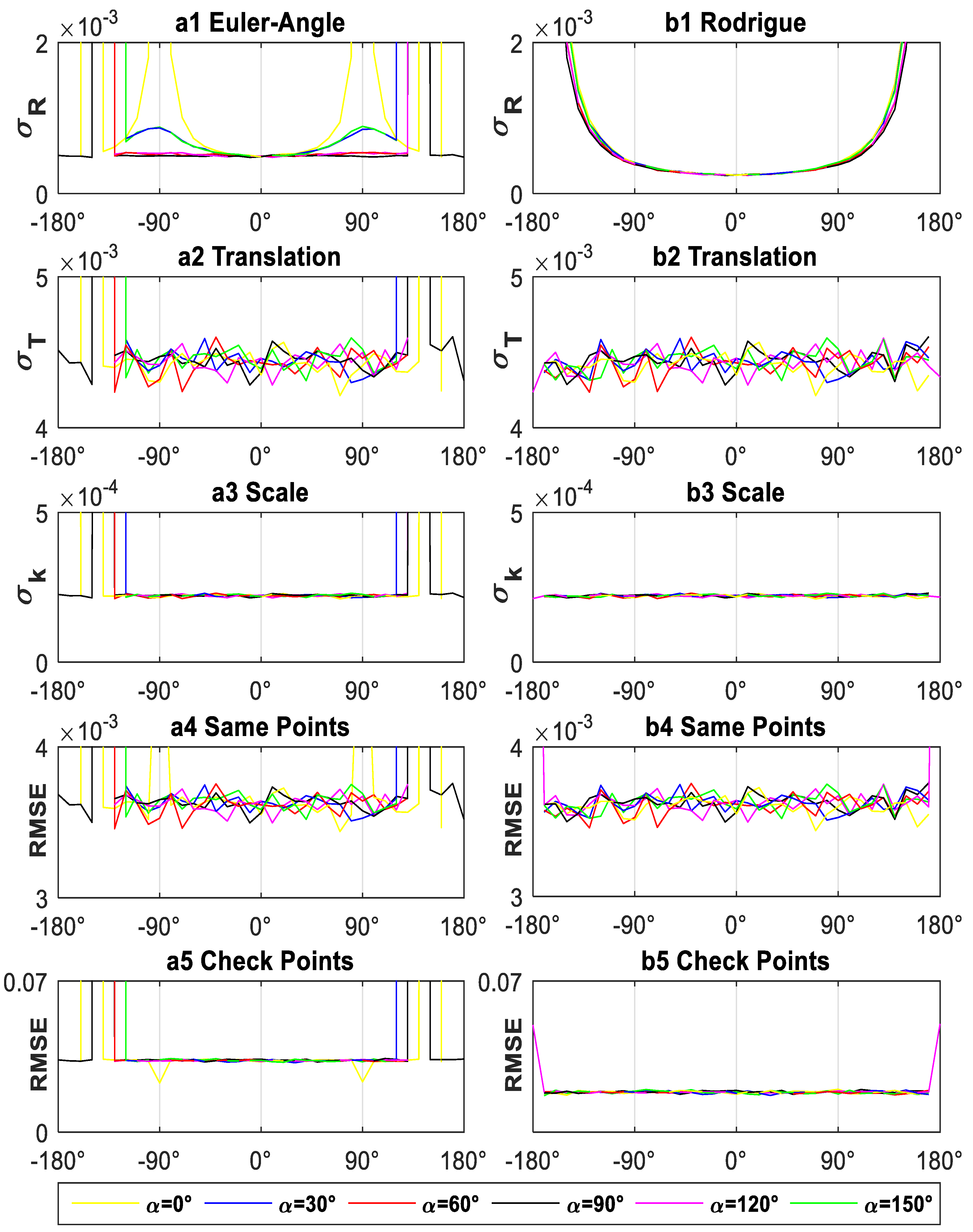
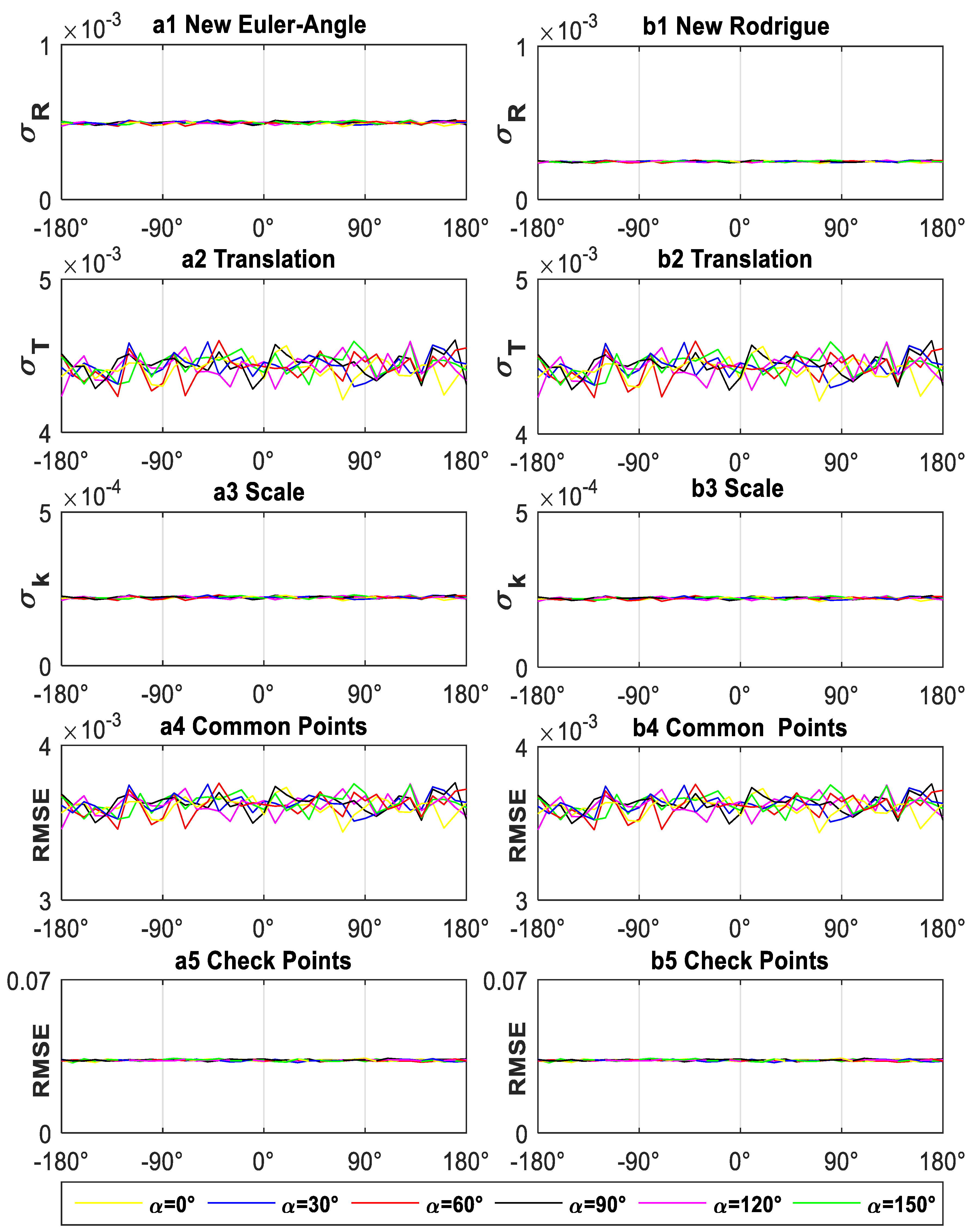
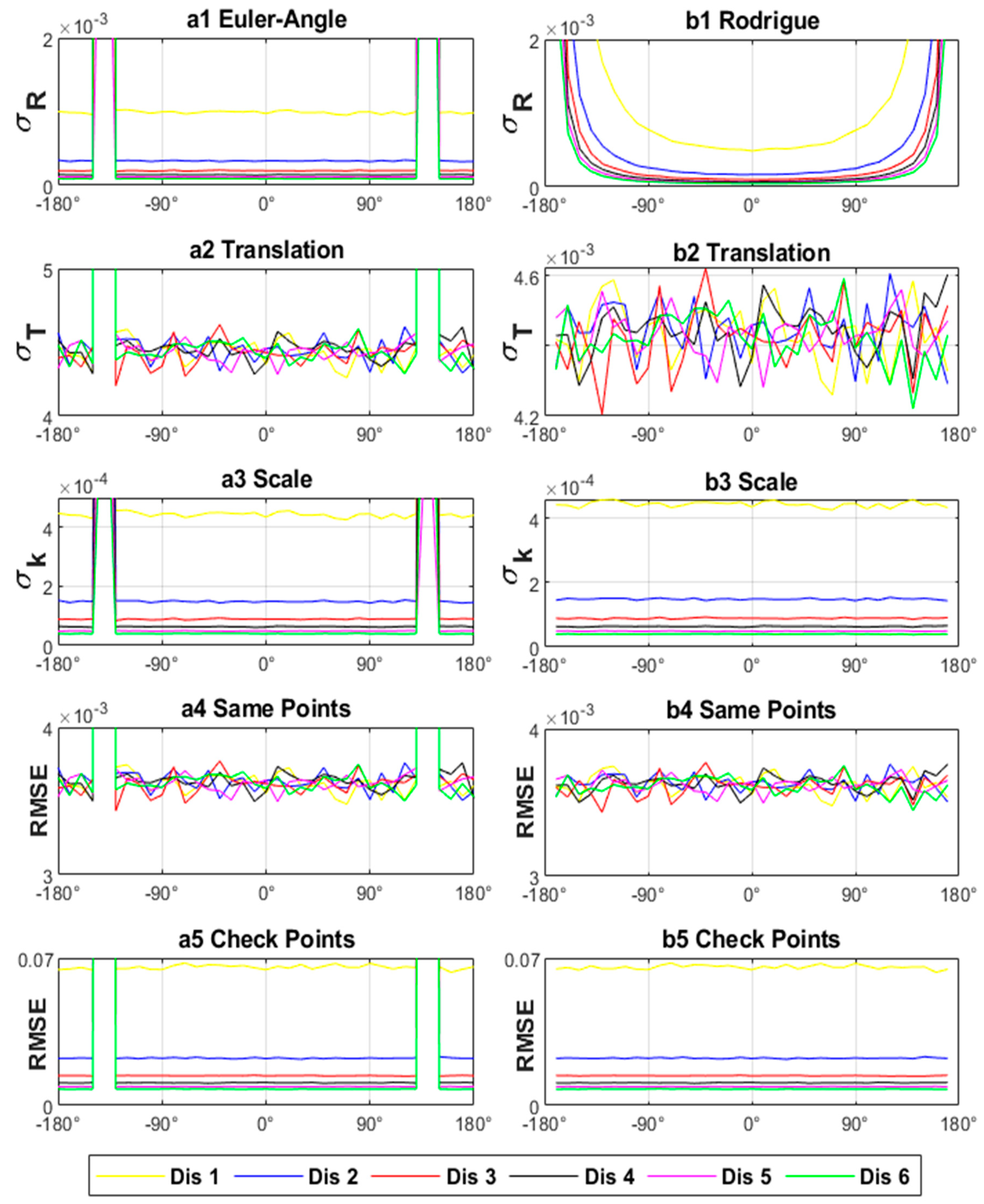
3. Experiments and Discussion

In this part, we set a series of simulation experiments and a practical engineering experiment to demonstrate the usability and efficiency of our proposed model. We first introduce the constraints for the simulation experiments and the simulation method. Then, we give a practical engineering experimental approach. Finally, we analyze the two current transformation models and the two new transformation models with the results of the experiments.

3.1. Constraint Conditions

Without affecting the conclusion of the simulation experiments, we make some assumptions: (1) The errors of the coordinates of common points and check points in coordinate system-(i + 1) are not considered in this paper; (2) unit weight variance σ 0 = 5   mm , since the size of σ 0 dose not affect the relative relationship between different values of different evaluation indices, and many laser scanner acquisition error = 5 mm@50 m [10]; (3) the threshold value T h r k of the translation parameters is 10 4 (equivalent to 0.1 mm), the threshold value T h r k of the rotation parameters is 10 9 (equivalent to less than 0.001″), and the threshold value T h r k of the scale parameters is 10 8 (equivalent to less than 0.1   mm / 100   km ) [14]; (4) the check points are the same in Experiment I and Experiment II; and (4) the unit weight is used in all of the experiments in this paper.

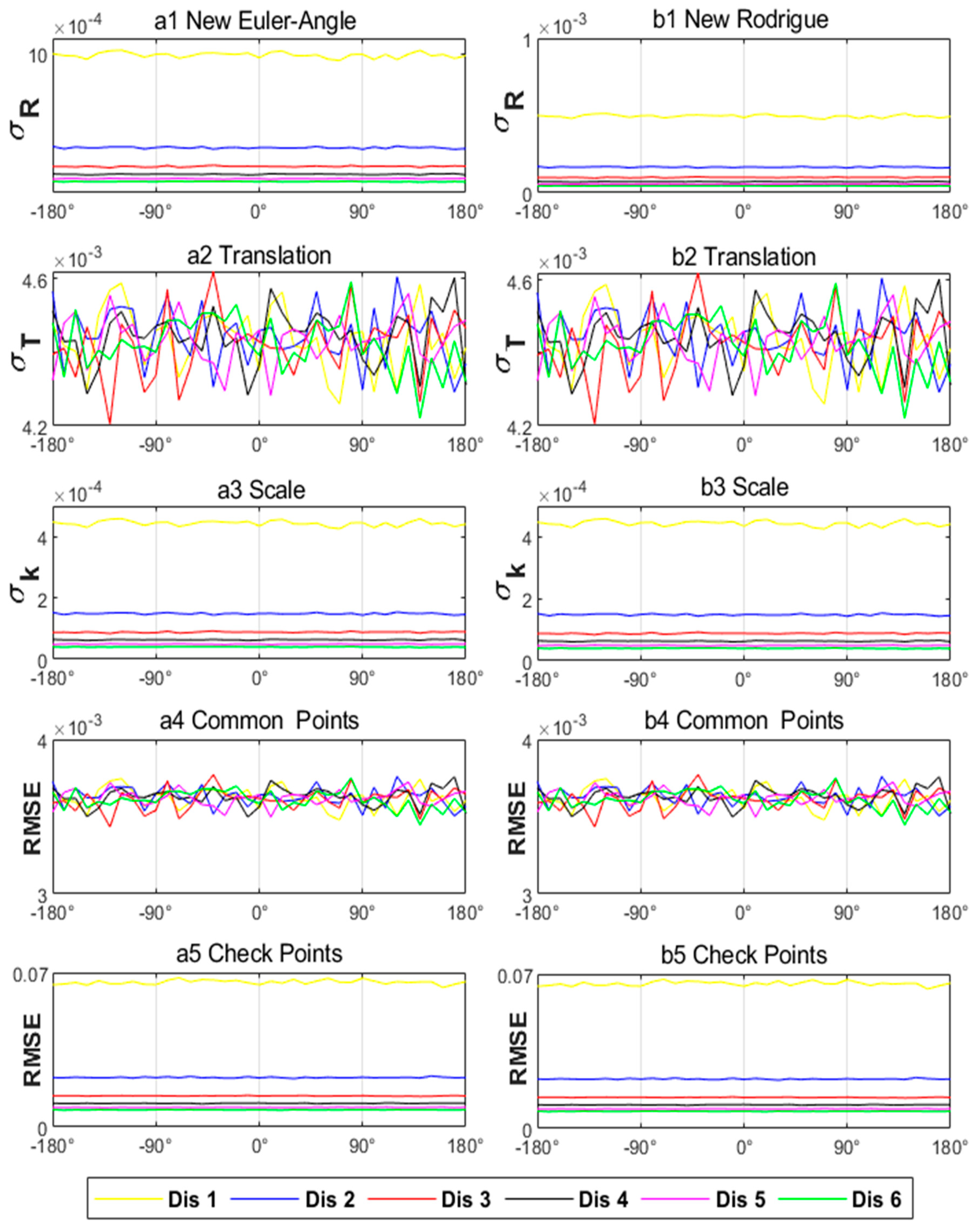
3.2. Simulation Experiments

We generate the rotation matrices with different rotation angles and different fixed rotation axes, and 1000 sets of coordinates of common points and check points in coordinate system-i are randomly simulated by the common points and check points in experiment I (see Table 1, different rotation axes α , different rotation angles δ , same common points, same check points). Then, we calculate the mean value of five transformation precision indices σ R , σ T , σ k , R M S E s a m e , and R M S E c h e c k of the Euler angle method (EA-Method, see Appendix B), Rodrigue method (R-Method, see Appendix C), new Euler angle method (NEA-Method, see Section 2.3), and new Rodrigue method (NR-Method, see Section 2.3) using the procedure shown in Appendix D. Similarly, we generate the rotation matrices with different rotation angles, different fixed common points distributions, and a fixed rotation axis, and randomly simulate 1000 sets of coordinates of common points and check points in coordinate system-I by the coordinates of common points and check points in experiment II (see Table 1, fixed rotation axes α , different rotation angles δ , different common points, same check points). We calculate the mean value of σ R , σ T , σ k , R M S E s a m e , and R M S E c h e c k of EA-Method, R-Method, NEA-Method, and NR-Method using the procedure shown in Appendix D. The specific experimental procedure is summarized as follows:
Step 1: Assume the total number of the common points n = 3 ; the total number of the check points m = 9 ; and the angle between the rotation axis n and the plane X O Y of Coordinate system-(i + 1) is α (corresponding to different rotation axes);
Step 2: Input the weight matrix P and the coordinates of common points and check points in Experiment I;
Step 3: Let α = 0 , π 6 , 2 π 6 , 3 π 6 , 4 π 6 , 5 π 6 . The EA-Method and the R-Method are separately used to calculate the mean value of σ R , σ T , σ k , R M S E s a m e , and R M S E c h e c k for different fixed rotation axes and different rotation angles using the procedure shown in Appendix D (see Figure 1);
Step 4: Let α = 0 , π 6 , 2 π 6 , 3 π 6 , 4 π 6 , 5 π 6 . The NEA-Method and the NR-Method are separately used to calculate the mean value of σ R , σ T , σ k , R M S E s a m e , and R M S E c h e c k for different fixed rotation axes and different rotation angles using the procedure shown in Appendix D (see Figure 2);
Step 5: Input P and the coordinates of common points and check points in Experiment II;
Step 6: Let α = π 2 . The EA-Method and the R-Method are separately used to calculate the mean value of σ R , σ T , σ k , R M S E s a m e , and R M S E c h e c k for different common points distributions using the procedure shown in Appendix D (see Figure 3);
Step 7: Let α = π 2 . The NEA-Method and the NR-Method are separately used to calculate the mean value of σ R , σ T , σ k , R M S E s a m e , and R M S E c h e c k for different common points distributions using the procedure shown in Appendix D (Figure 4).

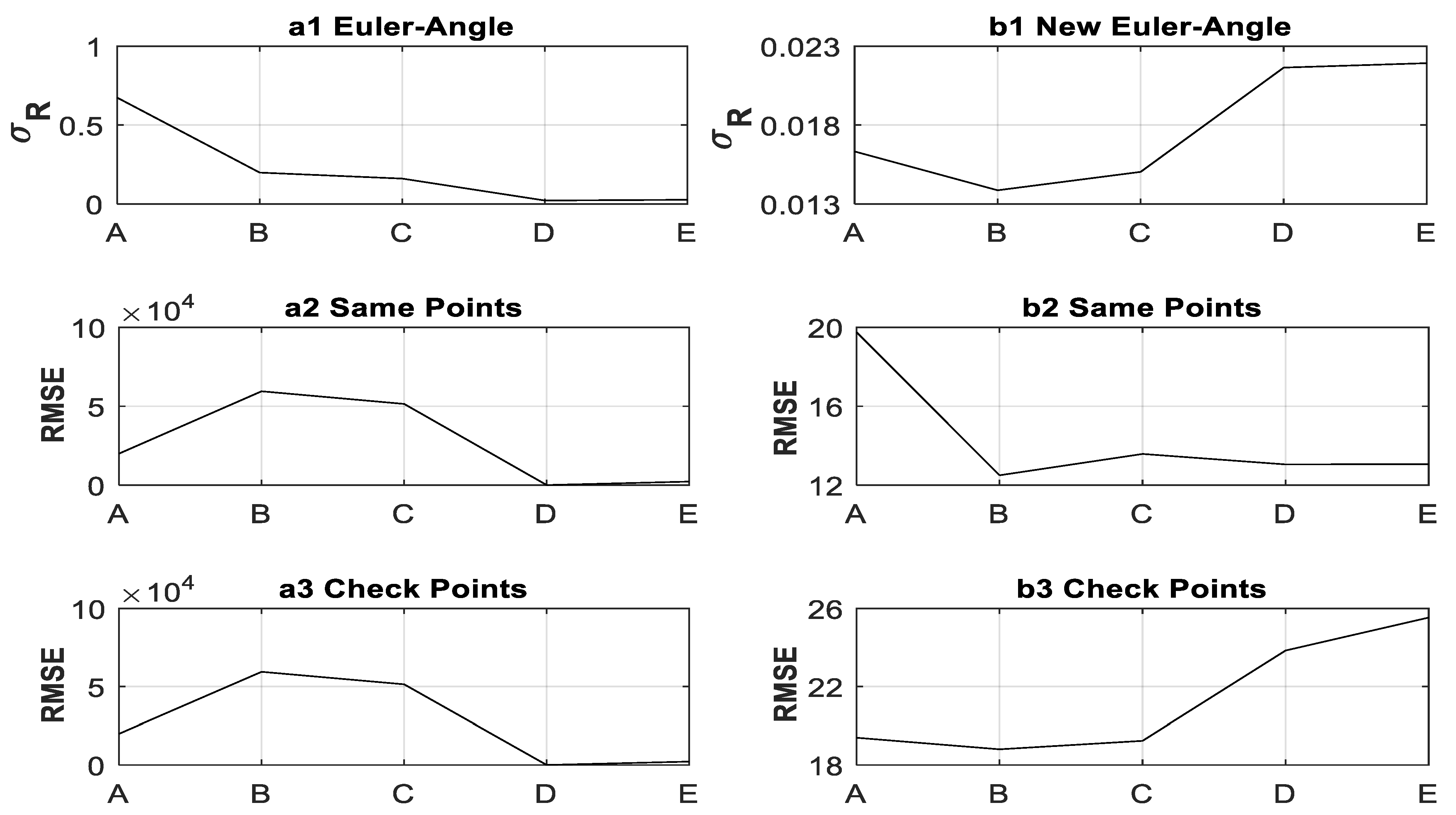
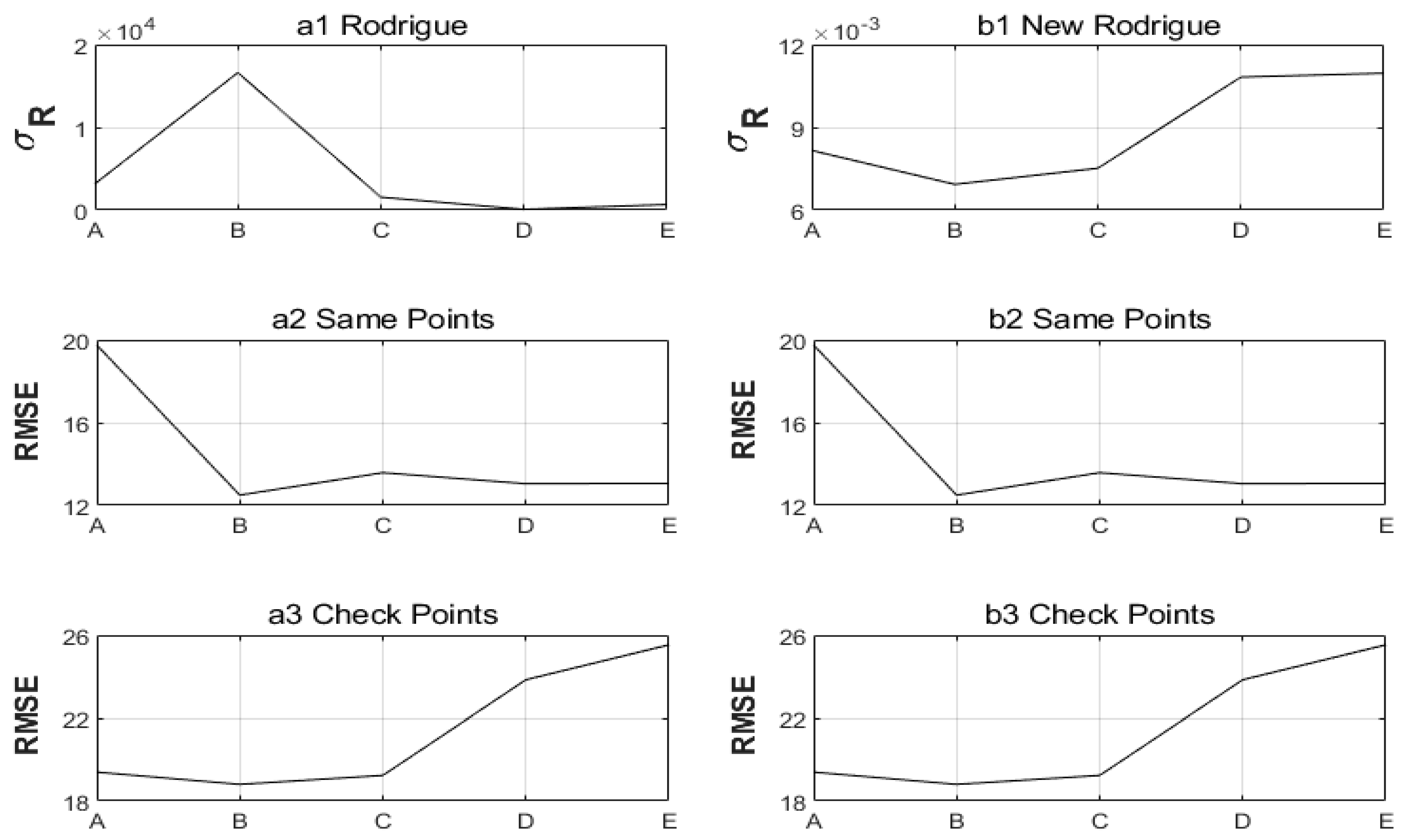
3.3. Practical Engineering Case

To further verify the applicability of the proposed method described in Section 2.3 we selected a dataset from a practical engineering application in Guangzhou’s new airport terminal [1,15], which consists of the true coordinates and measured coordinates of 15 nodes and 2 hinge center points in a component of the grid structure, as shown in Table 2. The origin in the true coordinates and the measured coordinates are the center of the end hinge of the component and any hypothetical point, respectively. In total, 5 cases are considered in this study, each of which selects 5 out of 17 points as common points: Case A selects {1, 11, 12, 13, 23}; Case B selects {1, 8, 9, 10, 23}; Case C selects {1, 14, 15, 16, 23}; Case D selects {1, 5, 6, 7, 23}; and Case E selects {1, 17, 18, 19, 23}. We then calculate σ R , R M S E s a m e , and R M S E c h e c k by the EA-Method, R-Method, NEA-Method, and NR-Method, respectively. The detailed experimental procedure is summarized as follows:
Step 1: Let the number of common points and check points be n = 5 and m = 17 , respectively;
Step 2: Input P , the coordinate of 17 position points in Table 2;
Step 3: Let the coordinate of common points be Case A, Case B, Case C, Case D, and Case E, respectively; the EA-Method and the NEA-Method are separately used to calculate the σ R , R M S E s a m e , and R M S E c h e c k using the procedure shown in Appendix B and the procedure in Section 2.3 (see Figure 5);
Step 4: Let the coordinate of common points be Case A, Case B, Case C, Case D, and Case E, respectively; the R-Method and the NR-Method are separately used to calculate the σ R , R M S E s a m e , and R M S E c h e c k using the procedure shown in Appendix C and the procedure in Section 2.3 (see Figure 6).

3.4. Discussion

From Figure 1 and Figure 3, it may be concluded that: (1) EA-Method becomes singular when the rotation angle is around 90° and 140°, and R-Method is singular when the rotation angle is close to 180°. Thus, the current EA-Method and R-Method are not suitable for estimating the transformation parameters in some circumstances. (2) RMSE of the common points and check points is independent of the rotation angle and rotation axis, but the rotation parameters’ precision σ R estimated by R-Method is related to the rotation axis and proportional to the absolute value of the rotation angle. Therefore, in the case where the rotation matrices are different, the small value of the rotation parameters’ estimation precision cannot represent that the corresponding transformation precision is better than the larger value of the rotation parameters’ estimation precision, and the rotation parameters’ precision estimated by R-Method is not suitable for evaluating the RMSE of the check points. (3) RMSE of the different common points in Experiment II can be considered the same, and the translation parameters’ precision σ T can also be considered the same, but the corresponding RMSE of the check points is not equal when different common points are used. Thus, the RMSE of the common points and the translation parameters’ precision all cannot be used to evaluate the RMSE of the check points.
From Figure 2 and Figure 4, it may be concluded that: (1) NEA-Method can resolve the singularity problem of EA-Method under some rotation angles, and NR-Method can also resolve the singularity problem of R-Method under the near 180° rotation angle; (2) the rotation parameters’ precision σ R estimated by NEA-Method and that by NR-Method is independent of the rotation angle and the rotation axis, so the evaluation indices of σ R estimated by NEA-Method and NR-Method are unique to different coordinate transformations; and (3) the rotation parameters’ precision σ R estimated by NEA-Method and that by NR-Method is proportional to the RMSE of the check points. Thus, the evaluation indices of σ R estimated by NEA-Method and NR-Method can be used to evaluate the RMSE of the check points.
From Figure 5 and Figure 6, several observations can be made as follows:(1) EA-Method still has singularity for A, B, and C distributions, where the RMSE of the common points and check points are more than 10,000 mm, so EA-Method is not suitable for this experiment; (2) the RMSE of the check points for NE-Method, R-Method, and NR-Method in the same case are equal, and its RMSE values for case A, B, C, D, and E are 19.4, 18.8, 19.2, 23.9, and 25.5 mm, respectively (the size is comparable to the calculated value in the literature [1,15], the results are correct), respectively, where the size relationship is E > D > A > C > B (see subgraph Figure 5b3 and Figure 6a3,b3); that is, “the size relationship of the check points’ RMSE is inconsistent with that of the common points’ RMSE”, so the RMSE of the check points cannot be used to evaluate the RMSE of the common points; (3) the RMSE values of the common points for NE-Method, R-Method, and NR-Method in the same case are also equal, but its RMSE values for case A, B, C, D, and E are 19.8, 12.5, 13.6, 13.05, and 13.06 mm, respectively, where the size relationship is A > C > E > D > B (see subgraph Figure 5b2 and Figure 6a2,b2); that is, “the size relationship of the common points’ RMSE is inconsistent with that of the check points’ RMSE”, so the RMSE of the common points cannot be used to evaluate the RMSE of the check points; (4) for NEA-Method and NR-Method, the size relationship of σ R in case A, B, C, D, E is E > D > A > C > B (see subgraph Figure 5b1), and for R-Method, the size relationship is B > A > C > E > D (see subgraph Figure 6a1; that is, “the size relationship of σ R calculated by R-Method is inconsistent with that of the check points’ RMSE, and the size relationship of σ R calculated by NEA-Method and NR-Method is consistent with that of the check points’ RMSE”, so the rotation parameters’ precision calculated by NEA-Method and NR-Method is suitable for evaluating the size relationship of the different check points’ RMSE but that by R-Method is not.

4. Conclusions

Motivated by the observation that the current coordinate transformation models’ have some limitations, this paper proposed a new method for coordinate transformation to deal with these limitations. The new transformation method was constructed by using the orthogonality of rotation matrix, the theorem of “any vector multiplied by the identity matrix does not change”, and the approximation of the rotation matrix (which is calculated by the orthogonal Procrustes method). The corresponding estimation formulas of th new transformation method were derived from the linearization theorem, the partial derivation theorem of matrix, and the principle of least squares adjustment.
We designed two simulation experiments and a practical engineering case to verify the effectiveness and applicability of the new transformation method. The results demonstrated that (1) the new transformation model is suitable for the Cartesian coordinate transformation under any rotation angle; (2) the rotation parameters’ precision calculated by the new method can be used to evaluate the transformation precision; (3) the new transformation method can be used to resolve the evaluation problem in the absence of check points.
However, it should be noted that “we do not consider the effects of linearization errors or coefficient matrix errors”; “our method only evaluates the accuracy of conversion parameters while the accuracy of any point in space is related to the accuracy of parameter conversion, the coordinates of any point, and the measurement accuracy of coordinates of any point and when calculating the accuracy of any point in space, it is necessary to refer to the related formula in [22]”; and “the relationship between the accuracy of conversion parameters and the accuracy of the final converted results requires further analytical investigation”.

Author Contributions

R.Y. was the scientific responsible and coordinator of the research group, and responsible for the derivation of relevant theories in the paper; R.Y., C.D., K.Y. and Z.L. conceived the original ideas; R.Y. and L.P. worked on preparing the original draft; K.Y. and C.D. assisted in results compiling and writing the manuscript; R.Y. and Z.L. supervised the research work. All authors have read and agreed to the published version of the manuscript.

Funding

This research is supported by the Chongqing Natural Science Foundation (No. cstc2019jcyj-msxmX0153), the 111 projects (No. B18062), the National Natural Science Foundation of China (No. 41304001 and No. 41674005), and the Fundamental Research Funds for the Central Universities (No.02180052020026).

Data Availability Statement

The datasets and source codes used in this study is available from the corresponding author on a reasonable request.

Acknowledgments

The authors would like to thank all anonymous reviewers for their valuable, constructive, and prompt comments and suggestions. And we appreciate Yi Chen, Yunzhong Shen, Dajie Liu, Huaien Zeng and Shengxiang Huang for their contribution and support in field data collection.

Conflicts of Interest

The authors declare no conflict of interest.

Appendix A. Calculation of Approximate Transformation Parameters by the Orthogonal Procrustes Method

We can compute the approximation k 0 , ω x 0 , ω y 0 , ω z 0 , a 0 , b 0 , c 0 , t x 0 , t y 0 , t z 0 of scale parameter k ; rotation parameters ω x , ω y , ω z , a , b , c ; and translation parameters t x , t y , t z by the orthogonal Procrustes method, which was given in [16]. The specific steps are as follows [16]:
Step 1: Constituting the common points matrix H A and H B based on all the common points’ coordinates:
H A ( j , : ) = [ x j i + 1 y j i + 1 z j i + 1 ] ,   H B ( j , : ) = [ x j i y j i z j i ] ,   j = 1 , , n ,
where n is the total number of the common points;
Step 2: Computing orthogonal matrices U and V by singular value decomposition:
U V T = s v d ( H A T ( E n 1 n e n e n T ) H B ) ,
where:
E n = [ 1 1 1 ] ,   e n = [ 1 1 1 ] ,
Step 3: Computing the approximation of rotation matrix and rotation parameters:
R i + 1 , 0 = V U T | V U T | ,
{ ω y 0 = arcsin ( R i + 1 , 0 ( 3 , 1 ) ) ω x 0 = arcsin ( R i + 1 , 0 ( 3 , 2 ) cos ω y 0 ) ω z 0 = arcsin ( R i + 1 , 0 ( 2 , 1 ) cos ω y 0 ) ,   { a 0 = R i + 1 , 0 ( 2 , 3 ) R i + 1 , 0 ( 3 , 2 ) t r ( R i + 1 , 0 ) + 1 b 0 = R i + 1 , 0 ( 3 , 1 ) R i + 1 , 0 ( 1 , 3 ) t r ( R i + 1 , 0 ) + 1 c 0 = R i + 1 , 0 ( 1 , 2 ) R i + 1 , 0 ( 2 , 1 ) t r ( R i + 1 , 0 ) + 1 ;
Step 4: Computing the approximation of the scale parameter:
k 0 = t r ( R i + 1 , 0 H A T ( E n × n 1 n e n e n T ) H B ) t r ( H A T ( E n × n 1 n e n e n T ) H A ) ;
Step 5: Computing the approximation of the translation parameters:
T 0 = [ t x 0 t y 0 t z 0 ] = 1 n ( H B T k 0 R i + 1 , 0 H A T ) e n .

Appendix B. Euler Angle Method

If the rotation matrix is expressed by three Euler angle parameters ( ω x , ω y , ω z ) (see Equation (2)), using Equations (1)–(3), with the approximations k 0 , ω x 0 , ω y 0 , ω z 0 , t x 0 , t y 0 , t z 0 and all the common points { p j i , p j i + 1 } j = 1 , , n , we can construct the error equation of the seven-parameter transformation model based on the Euler angle [8]:
V ω = B ω x ω l ω ,
where V ω is the 3 n × 1 residual matrix, B ω is the 3 n × 7 coefficient matrix, x ω is the true errors of the approximations X ω 0 = [ t x 0 t y 0 t z 0 ω x 0 ω y 0 ω z 0 k 0 ] T , l ω is the 3 n × 1 matrix, and:
x ω = [ d t x d t y d t z d ω x d ω y d ω z d k ] T ,
V ω = [ v ω 1 v ω n ] ,   v ω j = B ω j x l ω j ,   j = 1 , , n ,
l ω = [ l ω 1 l ω n ] ,   l ω j = p j i k 0 R i + 1 , 0 p j i + 1 T 0 ,   T 0 = [ t x 0 t y 0 t z 0 ] ,   j = 1 , , n ,
B ω = [ B ω 1 B ω n ] ,   B ω j = [ E 3 × 3 R i + 1 ω x p j i + 1 R i + 1 ω y p j i + 1 R i + 1 ω z p j i + 1 R i + 1 , 0 p j i + 1 ] ,   j = 1 , , n ,
R i + 1 , 0 = [ r 0 ( 11 ) r 0 ( 12 ) r 0 ( 13 ) r 0 ( 21 ) r 0 ( 22 ) r 0 ( 23 ) r 0 ( 31 ) r 0 ( 32 ) r 0 ( 33 ) ] ,   { r 0 ( 11 ) = cos ω y 0 cos ω z 0 r 0 ( 12 ) = cos ω x 0 sin ω z 0 + sin ω x 0 sin ω y 0 cos ω z 0 r 0 ( 13 ) = sin ω x 0 sin ω z 0 cos ω x 0 sin ω y 0 cos ω z 0 r 0 ( 21 ) = cos ω y 0 sin ω z 0 r 0 ( 22 ) = cos ω x 0 cos ω z 0 sin ω x 0 sin ω y 0 sin ω z 0 r 0 ( 23 ) = sin ω x 0 cos ω z 0 + cos ω x 0 sin ω y 0 sin ω z 0 r 0 ( 31 ) = sin ω y 0 r 0 ( 32 ) = sin ω x 0 cos ω y 0 r 0 ( 33 ) = cos ω x 0 cos ω y 0 ,
R i + 1 ω x = [ 0 r x ( 12 ) r x ( 13 ) 0 r x ( 22 ) r x ( 23 ) 0 r x ( 32 ) r x ( 33 ) ] ,   { r x ( 12 ) = sin ω x 0 sin ω z 0 + cos ω x 0 sin ω y 0 cos ω z 0 r x ( 13 ) = cos ω x 0 sin ω z 0 + sin ω x 0 sin ω y 0 cos ω z 0 r x ( 22 ) = sin ω x 0 cos ω z 0 cos ω x 0 sin ω y 0 sin ω z 0 r x ( 23 ) = cos ω x 0 cos ω z 0 sin ω x 0 sin ω y 0 sin ω z 0 r x ( 32 ) = cos ω x 0 cos ω y 0 r x ( 33 ) = sin ω x 0 cos ω y 0 ,
R i + 1 ω y = [ r y ( 11 ) r y ( 12 ) r y ( 13 ) r y ( 21 ) r y ( 22 ) r y ( 23 ) r y ( 31 ) r y ( 32 ) r y ( 33 ) ] ,   { r y ( 11 ) = sin ω y 0 cos ω z 0 r y ( 12 ) = sin ω x 0 cos ω y 0 cos ω z 0 r y ( 13 ) = cos ω x 0 cos ω y 0 cos ω z 0 r y ( 21 ) = sin ω y 0 sin ω z 0 r y ( 22 ) = sin ω x 0 cos ω y 0 sin ω z 0 r y ( 23 ) = cos ω x 0 cos ω y 0 sin ω z 0 r y ( 31 ) = cos ω y 0 r y ( 32 ) = sin ω x 0 sin ω y 0 r y ( 33 ) = cos ω x 0 sin ω y 0 ,
R i + 1 ω z = [ r z ( 11 ) r z ( 12 ) r z ( 13 ) r z ( 21 ) r z ( 22 ) r z ( 23 ) 0 0 0 ] ,   { r z ( 11 ) = cos ω y 0 sin ω z 0 r z ( 12 ) = cos ω x 0 cos ω z 0 sin ω x 0 sin ω y 0 sin ω z 0 r z ( 13 ) = sin ω x 0 cos ω z 0 + cos ω x 0 sin ω y 0 sin ω z 0 r z ( 21 ) = cos ω y 0 cos ω z 0 r z ( 22 ) = cos ω x 0 sin ω z 0 sin ω x 0 sin ω y 0 cos ω z 0 r z ( 23 ) = sin ω x 0 sin ω z 0 + cos ω x 0 sin ω y 0 cos ω z 0 .
We can compute the estimated transformation parameters and the transformation precision evaluation index by the following steps [8]:
Step 1: Input the weight matrix P , the coordinates of the common points p j 1 i and p j 1 i + 1 , and the check points p j 2 i and p j 2 i + 1 in coordinate system-i and coordinate system-(i + 1), and the numbers of the common points and check points n and m , the estimation threshold values of the translation parameters, the rotation parameters, and the scale parameters T h r T , T h r R , and T h r k ;
Step 2: Calculate the approximation value t x 0 , t y 0 , t z 0 , ω x 0 , ω y 0 , ω z 0 , k 0 of the seven transformation parameters by Equations (A1)–(A7), and let X ω 0 = [ t x 0 t y 0 t z 0 ω x 0 ω y 0 ω z 0 k 0 ] T ;
Step 3: Calculate R i + 1 , 0 , R i + 1 ω x , R i + 1 ω y , R i + 1 ω z by Equations (A13)–(A16);
Step 4: Constitute the coefficient matrix B ω by Equation (A12);
Step 5: Constitute the matrix l ω by Equation (A11);
Step 6: Calculate the estimated values of x ω as
x ^ ω = ( B ω T P B ω ) 1 B ω T P l ω ;
Step 7: If x ^ ω is less than the given limit, which is max { abs { x ^ ω ( 1 : 3 ) } } T h T , max { abs { x ^ ω ( 4 : 6 ) } } T h R and max { abs { x ^ ω ( 7 ) } } T h k , continue; if not, X ω 0 = X ω 0 + x ^ ω , and go to Step 3;
Step 8: Calculate the estimated transformation parameters:
X ^ = X ω 0 + x ^ ω ,   T ^ i + 1 = [ t ^ x t ^ y t ^ z ] = [ X ^ ( 1 ) X ^ ( 2 ) X ^ ( 3 ) ] ,   [ ω ^ x ω ^ y ω ^ z ] = [ X ^ ( 4 ) X ^ ( 5 ) X ^ ( 6 ) ] ,   k ^ = X ^ ( 7 ) ,
R ^ i + 1 = [ r ^ ( 11 ) r ^ ( 12 ) r ^ ( 13 ) r ^ ( 21 ) r ^ ( 22 ) r ^ ( 23 ) r ^ ( 31 ) r ^ ( 32 ) r ^ ( 33 ) ] ,   { r ^ ( 11 ) = cos ω ^ y cos ω ^ z r ^ ( 12 ) = cos ω ^ x sin ω ^ z + sin ω ^ x sin ω ^ y cos ω ^ z r ^ ( 13 ) = sin ω ^ x sin ω ^ z cos ω ^ x sin ω ^ y cos ω ^ z r ^ ( 21 ) = cos ω ^ y sin ω ^ z r ^ ( 22 ) = cos ω ^ x cos ω ^ z sin ω ^ x sin ω ^ y sin ω ^ z r ^ ( 23 ) = sin ω ^ x cos ω ^ z + cos ω ^ x sin ω ^ y sin ω ^ z r ^ ( 31 ) = sin ω ^ y r ^ ( 32 ) = sin ω ^ x cos ω ^ y r ^ ( 33 ) = cos ω ^ x cos ω ^ y ,
where X ^ is the estimated values of the seven transformation parameters; T ^ i + 1 is the estimated values of the translation parameters; ω ^ x , ω ^ y , ω ^ z are the estimated values of the translation parameters; k ^ is the estimated values of the scale parameters; and R ^ i + 1 is the estimated values of the rotation matrix;
Step 9: Calculate the evaluation index of the transformation precision:
{ σ T = D X ω ( 1 , 1 ) + D X ω ( 2 , 2 ) + D X ω ( 3 , 3 ) σ R = D X ω ( 4 , 4 ) + D X ω ( 5 , 5 ) + D X ω ( 6 , 6 ) σ k = D X ω ( 7 , 7 ) ,
{ R M S E s a m e = 1 n j 1 = 1 n Δ ω j 1 2 R M S E c h e c k = 1 m j 2 = 1 m Δ ω j 2 2 ,
where σ T , σ R , and σ k are the evaluation indices of the translation parameters’ estimation precision, rotation parameters’ estimation precision, and scale parameter’ estimation precision, respectively; R M S E s a m e , R M S E c h e c k are the root mean square error of the common points and the check points, respectively; D X ω is the variance and covariance of the estimated transformation parameters; Δ ω j 1 and Δ ω j 2 are the transformation error of the common points and the check points, respectively; and:
D X ω = σ 0 2 ( B ω T P B ω ) 1 ,   Δ ω j 1 = p j 1 i k ^ R ^ i + 1 p j 1 i + 1 T ^ i + 1 ,   Δ ω j 2 = p j 2 i k ^ R ^ i + 1 p j 2 i + 1 T ^ i + 1 ,
where σ 0 is the unit weight variance (usually determined in the initial processing before transformation).

Appendix C. Rodrigue Method

If the rotation matrix is expressed by three Rodrigue parameters ( a , b , c ) (see Equation (3)), using Equations (1)–(3), with the approximations k 0 , a 0 , b 0 , c 0 , t x 0 , t y 0 , t z 0 , and all the common points { p j i , p j i + 1 } j = 1 , , n , we can construct the error equation of the seven-parameter transformation model based on Rodrigue parameters [4,22]:
V a b c = B a b c x a b c l a b c ,
where V a b c is the 3 n × 1 residual matrix, B a b c is the 3 n × 7 coefficient matrix, x a b c is the true errors of the approximations X a b c 0 = [ t x 0 t y 0 t z 0 a 0 b 0 c 0 k 0 ] T , l a b c is the 3 n × 1 matrix, and:
x a b c = [ d t x d t y d t z d a d b d c d k ] T ,
V a b c = [ v a b c 1 v a b c n ] ,   v a b c j = B a b c j x l a b c j ,   j = 1 , , n ,
l a b c = [ l a b c 1 l a b c n ] ,   l a b c j = p j i k 0 R i + 1 , 0 p j i + 1 T 0 ,   T 0 = [ t x 0 t y 0 t z 0 ] ,   j = 1 , , n ,
B a b c = [ B a b c 1 B a b c n ] ,   B a b c j = [ E 3 × 3 R i + 1 a p j i + 1 R i + 1 b p j i + 1 R i + 1 c p j i + 1 R i + 1 , 0 p j i + 1 ] ,   j = 1 , , n ,
R i + 1 , 0 = 1 1 + a 0 2 + b 0 2 + c 0 2 [ 1 + a 0 2 b 0 2 c 0 2 2 ( a 0 b 0 + c 0 ) 2 ( a 0 c 0 b 0 ) 2 ( a 0 b 0 c 0 ) 1 a 0 2 + b 0 2 c 0 2 2 ( b 0 c 0 + a 0 ) 2 ( a 0 c 0 + b 0 ) 2 ( b 0 c 0 a 0 ) 1 a 0 2 b 0 2 + c 0 2 ] ,
R i + 1 a = [ r a ( 11 ) r a ( 12 ) r a ( 13 ) r a ( 21 ) r a ( 22 ) r a ( 23 ) r a ( 31 ) r a ( 32 ) r a ( 33 ) ] ( 1 + a 0 2 + b 0 2 + c 0 2 ) 2 ,   { r a ( 11 ) = 4 a 0 ( b 0 2 + c 0 2 ) r a ( 12 ) = 2 b 0 ( 1 a 0 2 + b 0 2 + c 0 2 ) 4 a 0 c 0 r a ( 13 ) = 2 c 0 ( 1 a 0 2 + b 0 2 + c 0 2 ) + 4 a 0 b 0 r a ( 21 ) = 2 b 0 ( 1 a 0 2 + b 0 2 + c 0 2 ) + 4 a 0 c 0 r a ( 22 ) = 4 a 0 ( 1 + b 0 2 ) r a ( 23 ) = 2 ( 1 a 0 2 + b 0 2 + c 0 2 ) 4 a 0 b 0 c 0 r a ( 31 ) = 2 c 0 ( 1 a 0 2 + b 0 2 + c 0 2 ) 4 a 0 b 0 r a ( 32 ) = 2 ( 1 a 0 2 + b 0 2 + c 0 2 ) 4 a 0 b 0 c 0 r a ( 33 ) = 4 a 0 ( 1 + c 0 2 ) ,
R i + 1 b = [ r b ( 11 ) r b ( 12 ) r b ( 13 ) r b ( 21 ) r b ( 22 ) r b ( 23 ) r b ( 31 ) r b ( 32 ) r b ( 33 ) ] ( 1 + a 0 2 + b 0 2 + c 0 2 ) 2 ,   { r b ( 11 ) = 4 b 0 ( 1 + a 0 2 ) r b ( 12 ) = 2 a 0 ( 1 + a 0 2 b 0 2 + c 0 2 ) 4 b 0 c 0 r b ( 13 ) = 2 ( 1 + a 0 2 b 0 2 + c 0 2 ) 4 a 0 b 0 c 0 r b ( 21 ) = 2 a 0 ( 1 + a 0 2 b 0 2 + c 0 2 ) + 4 b 0 c 0 r b ( 22 ) = 4 b 0 ( a 0 2 + c 0 2 ) r b ( 23 ) = 2 c 0 ( 1 + a 0 2 b 0 2 + c 0 2 ) 4 a 0 b 0 r b ( 31 ) = 2 ( 1 + a 0 2 b 0 2 + c 0 2 ) 4 a 0 b 0 c 0 r b ( 32 ) = 2 c 0 ( 1 + a 0 2 b 0 2 + c 0 2 ) + 4 a 0 b 0 r b ( 33 ) = 4 b 0 ( 1 + c 0 2 ) ,
R i + 1 c = [ r c ( 11 ) r c ( 12 ) r c ( 13 ) r c ( 21 ) r c ( 22 ) r c ( 23 ) r c ( 31 ) r c ( 32 ) r c ( 33 ) ] ( 1 + a 0 2 + b 0 2 + c 0 2 ) 2 ,   { r c ( 11 ) = 4 c 0 ( 1 + a 0 2 ) r c ( 12 ) = 2 ( 1 + a 0 2 + b 0 2 c 0 2 ) 4 a 0 b 0 c 0 r c ( 13 ) = 2 a 0 ( 1 + a 0 2 + b 0 2 c 0 2 ) + 4 b 0 c 0 r c ( 21 ) = 2 ( 1 + a 0 2 + b 0 2 c 0 2 ) 4 a 0 b 0 c 0 r c ( 22 ) = 4 c 0 ( 1 + b 0 2 ) r c ( 23 ) = 2 b 0 ( 1 + a 0 2 + b 0 2 c 0 2 ) 4 a 0 c 0 r c ( 31 ) = 2 a 0 ( 1 + a 0 2 + b 0 2 c 0 2 ) 4 b 0 c 0 r c ( 32 ) = 2 b 0 ( 1 + a 0 2 + b 0 2 c 0 2 ) + 4 a 0 c 0 r c ( 33 ) = 4 c 0 ( a 0 2 + b 0 2 ) .
We can compute the estimated transformation parameters and the transformation precision evaluation index by the following steps [4,22]:
Step 1: Input the weight matrix P , the coordinates of the common points p j 1 i and p j 1 i + 1 , and the check points p j 2 i and p j 2 i + 1 in coordinate system-i and coordinate system-(i + 1), the numbers of the common points and check points n and m, the estimation threshold values of the translation parameters, the rotation parameters, and the scale parameters T h r T , T h r R , and T h r k ;
Step 2: Calculate the approximation value t x 0 , t y 0 , t z 0 , a 0 , b 0 , c 0 , k 0 of the seven transformation parameters by Equations (A1)–(A7), and let X a b c 0 = [ t x 0 t y 0 t z 0 a 0 b 0 c 0 k 0 ] T ;
Step 3: Calculate R i + 1 , 0 , R i + 1 a , R i + 1 b , R i + 1 c by Equations (A28)–(A30);
Step 4: Constitute the coefficient matrix B a b c by Equation (A27);
Step 5: Constitute the matrix l a b c by Equation (A26);
Step 6: Calculate the estimated values of x a b c as:
x ^ a b c = ( B a b c T P B a b c ) 1 B a b c T P l a b c ,
Step 7: If x ^ a b c is less than the given limit, which is max { abs { x ^ a b c ( 1 : 3 ) } } T h T , max { abs { x ^ a b c ( 4 : 6 ) } } T h R , and max { abs { x ^ a b c ( 7 ) } } T h k , continue; if not, X a b c 0 = X a b c 0 + x ^ a b c , and go to Step 3;
Step 8: Calculate the estimated transformation parameters:
X ^ = X a b c 0 + x ^ a b c ,   T ^ i + 1 = [ t ^ x t ^ y t ^ z ] = [ X ^ ( 1 ) X ^ ( 2 ) X ^ ( 3 ) ] ,   [ a ^ b ^ c ^ ] = [ X ^ ( 4 ) X ^ ( 5 ) X ^ ( 6 ) ] ,   k ^ = X ^ ( 7 ) ,
R ^ i + 1 = 1 1 + a ^ 2 + b ^ 2 + c ^ 2 [ 1 + a ^ 2 b ^ 2 c ^ 2 2 ( a ^ b ^ + c ^ ) 2 ( a ^ c ^ b ^ ) 2 ( a ^ b ^ c ^ ) 1 a ^ 2 + b ^ 2 c ^ 2 2 ( b ^ c ^ + a ^ ) 2 ( a ^ c ^ + b ^ ) 2 ( b ^ c ^ a ^ ) 1 a ^ 2 b ^ 2 + c ^ 2 ] ,
where X ^ , T ^ i + 1 , k ^ , R ^ i + 1 are as defined in Appendix B; and a ^ , b ^ , c ^ are the estimated values of the rotation parameters;
Step 9: Calculate the evaluation index of the transformation precision:
{ σ T = D X a b c ( 1 , 1 ) + D X a b c ( 2 , 2 ) + D X a b c ( 3 , 3 ) σ R = D X a b c ( 4 , 4 ) + D X a b c ( 5 , 5 ) + D X a b c ( 6 , 6 ) σ k = D X a b c ( 7 , 7 ) ,
{ R M S E s a m e = 1 n j 1 = 1 n Δ a b c j 1 2 R M S E c h e c k = 1 m j 2 = 1 m Δ a b c j 2 2 ,
where σ T , σ R , σ k , R M S E s a m e , R M S E c h e c k , and σ 0 are as defined in Appendix B; D X a b c is the variance and covariance of the estimated transformation parameters; and Δ a b c j 1 and Δ a b c j 2 are the transformation error of the common points and the check points, respectively; and:
D X a b c = σ 0 2 ( B a b c T P B a b c ) 1 ,   Δ a b c j 1 = p j 1 i k ^ R ^ i + 1 p j 1 i + 1 T ^ i + 1 ,   Δ a b c j 2 = p j 2 i k ^ R ^ i + 1 p j 2 i + 1 T ^ i + 1 .

Appendix D. Calculation Procedure of the Transformation Precision Index for Different Rotation Angles

Assume the angle α between the rotation axis n and the plane X O Y of coordinates-i + 1 is fixed, σ 0 = 5   mm . We can compute the transformation precision evaluation index of different rotation angles by the following steps:
Step 1: Assume k ˜ = 1 , T ˜ i + 1 = [ 10 10 10 ] T , δ = π ;
Step 2: Input the weight matrix P , the coordinates of the common points p ˜ j 1 i + 1 , the check points p ˜ j 2 i + 1 in coordinate system-i and coordinate system-(i + 1), and the numbers of the common points and check points n and m ;
Step 3: If δ π , j 0 = 1 , continue; if not, go to Step 10;
Step 4: Let the rotation parameters a ˜ = 0 , b ˜ = tan δ cos α , c ˜ = tan δ sin α , and calculate the coordinate true values of the common points and check points as:
p ˜ j 1 i = k ˜ R ˜ i + 1 p ˜ j 1 i + 1 + T ˜ i + 1 ,   p ˜ j 2 i = k ˜ R ˜ i + 1 p ˜ j 2 i + 1 + T ˜ i + 1 ,   j 1 = 1 , , n ,   j 2 = 1 , , m ,
where:
R ˜ i + 1 = 1 1 + a ˜ 2 + b ˜ 2 + c ˜ 2 [ 1 + a ˜ 2 b ˜ 2 c ˜ 2 2 ( c ˜ + a ˜ b ˜ ) 2 ( a ˜ c ˜ b ˜ ) 2 ( a ˜ b ˜ c ˜ ) 1 a ˜ 2 + b ˜ 2 c ˜ 2 2 ( a ˜ + b ˜ c ˜ ) 2 ( b ˜ + a ˜ c ˜ ) 2 ( b ˜ c ˜ a ˜ ) 1 a ˜ 2 b ˜ 2 + c ˜ 2 ] ;
Step 5: If j 0 1000 , continue; if not, go to Step 8;
Step 6: Add random noise to the coordinates of the common points in experiment I:
p j 1 i = p ˜ j 1 i + n o r m r n d ( 0 , σ 0 , 3 , 1 ) ,   j 1 = 1 , , n ,
where n o r m r n d ( 0 , σ 0 , 3 , 1 ) returns a 3 × 1 array of random numbers chosen from a normal distribution with a mean and standard deviation of 0 and σ 0 ;
Step 7: Calculate the σ R , j 0 , σ T , j 0 , σ k , j 0 , R M S E s a m e , j 0 , R M S E c h e c k , j 0 by the Euler-Angle-Method in Appendix B, Rodrigue-Method in Appendix C, or New-Transformation-Method in Section 2.3;
Step 8: Let j 0 = j 0 + 1 , and go to Step 5;
Step 9: Calculate the mean value of the transformation precision evaluation index:
σ R = j 0 = 1 1000 σ R , j 0 1000 ,   σ T = j 0 = 1 1000 σ T , j 0 1000 ,   σ k = j 0 = 1 1000 σ k , j 0 1000 ,   { R M S E s a m e = j 0 = 1 1000 R M S E s a m e , j 0 1000 R M S E c h e c k = j 0 = 1 1000 R M S E c h e c k , j 0 1000 ;
Step 10: δ = δ + π 18 , go to Step 3;
Step 11: End.

References

  1. Chen, Y.; Shen, Y.Z.; Liu, D.J. A simplified model of three dimensional-datum transformation adapted to big rotation angle. Geomat. Inf. Sci. Wuhan Univ. 2004, 29, 1101–1104. [Google Scholar]
  2. Luo, C.L.; Zhang, Z.L.; Deng, Y.; Mei, W.S.; Chen, B.R. On nonlinear 3D rectangular coordinate transformation method based on improved Gauss-Newton method. J. Geod. Geodyn. 2007, 27, 50–54. [Google Scholar]
  3. Qin, S.W.; Gu, C.; Pan, G.R. A simple and convenient coordinate transformation model for any rotation angle. Geotech. Inverstigation Surv. 2009, 62–65. [Google Scholar]
  4. Yao, J.L.; Han, B.M.; Yang, Y.X. Application of Lodrigues Matrix in 3D coordinate transformation. Geomat. Inf. Sci. Wuhan Univ. 2006, 31, 1094–1119. [Google Scholar] [CrossRef]
  5. Li, B.F.; Shen, Y.Z.; Li, W.X. The seamless model for three-dimensional datum transformation. Sci. China Earth Sci. 2012, 55, 2099–2108. [Google Scholar] [CrossRef]
  6. Li, B.F.; Huang, S.Q. Analytical close-form solutions for three-dimensional datum transformation with big rotation angles. Acta Geod. Et Cartogr. Sin. 2016, 45, 267–273. [Google Scholar]
  7. Eggert, D.W.; Lorusso, A.; Fisher, R.B. Estimating 3-D rigid body transformations: A comparison of four major algorithms. Mach. Vis. Appl. 1997, 9, 272–290. [Google Scholar] [CrossRef]
  8. Yao, Y.B.; Huang, C.M.; Li, C.C.; Kong, J. A new algorithm for solution of transformation parameters of big rotation angle’s 3D coordinate. Geomat. Inf. Sci. Wuhan Univ. 2012, 37, 253–256. [Google Scholar]
  9. Liu, Z.P.; Yang, L. An improved method for spatial rectangular coordinate transformation with big rotation angle. J. Geod. Geodyn. 2016, 36, 586–590. [Google Scholar]
  10. Yang, R.H. Research on Point Cloud Angular Resolution and Processing Model of Terrestrial Laser Scanning. Ph.D. Thesis, Wuhan University, Wuhan, China, 2011. [Google Scholar]
  11. Yang, R.H.; Meng, X.L.; Xiang, Z.J.; Li, Y.M.; You, Y.S. Establishment of a new quantitative evaluation model of the targets geometry distribution for terrestrial laser scanning. Sensors 2020, 20, 555. [Google Scholar] [CrossRef] [PubMed] [Green Version]
  12. Li, Z.W.; Li, K.Z.; Zhao, L.J.; Wang, Y.K.; Liang, X.Q. Three-dimensional coordinate transformation adapted to arbitrary rotation angles based on unit quaternion. J. Geod. Geodyn. 2017, 37, 81–85. [Google Scholar]
  13. Lin, P. The Method of Total Least Squares for 3d Datum Transformation in the Arbitrary Rotational Angle. Master’s Thesis, Anhui University of Science and Technology, Huainan, China, 2015. [Google Scholar]
  14. Zeng, W.X.; Tao, B.Z. Non-linear adjustment model of three-dimensional coordinate transformation. Geomat. Inf. Sci. Wuhan Univ. 2003, 28, 566–568. [Google Scholar]
  15. Zeng, H.E.; Huang, S.X. A kind of direct search method adapted to solution of 3d coordinate transformation parameters. Geomat. Inf. Sci. Wuhan Univ. 2008, 33, 1118–1121. [Google Scholar]
  16. Wu, J.Z.; Wang, A.Y. A unified model for cartesian coordinate transformations in two- and three-dimensional space. J. Geod. Geodyn. 2015, 35, 1046–1048, 1052. [Google Scholar]
  17. Li, M.F.; Liu, Z.L.; Wang, Y.M.; Sun, X.R. Study on an improved model for ill-conditioned three-dimensional coordinate transformation with big rotation angles. J. Geod. Geodyn. 2017, 37, 441–445. [Google Scholar]
  18. Chen, Z.Y.; Liu, C. Spatial coordinate transformation based on multiple parameter regularization and its accuracy analysis. J. Geod. Geodyn. 2008, 28, 92–95. [Google Scholar]
  19. Fang, X.; Zeng, W.X.; Liu, J.N.; Yao, Y.B. A general total least squares algorithm for three-dimensional coordinate transformations. Geomat. Inf. Sci. Wuhan Univ. 2014, 43, 1139–1143. [Google Scholar]
  20. Chen, Y.; Lu, J. Performing 3D similarity transformation by robust total least squares. Acta Geod. Et Cartogr. Sin. 2012, 41, 715–722. [Google Scholar]
  21. Fan, L.; Smethurst, J.A.; Atkinson, P.M.; Powrie, W. Error in target-based georeferencing and registration in terrestrial laser scanning. Comput. Geosci. 2015, 83, 54–64. [Google Scholar] [CrossRef] [Green Version]
  22. Yang, R.H.; Meng, X.L.; Yao, Y.B.; Chen, B.Y.; You, Y.S.; Xiang, Z.J. An analytical approach to evaluate point cloud registration error utilizing targets. ISPRS J. Photogramm. Remote Sens. 2018, 143, 48–56. [Google Scholar] [CrossRef]
  23. Liu, J. Research on Attitude Determination by Quaternion Method. Bachelor’s Thesis, Wuhan University, Wuhan, China, 2003. [Google Scholar]
  24. Qiu, W.N.; Tao, B.Z.; Yao, Y.B.; Wu, Y.; Huang, H.L. The Theory and Method of Surveying Data Processing, 1st ed.; Wuhan University Press: Wuhan China, 2008; pp. 1–6. [Google Scholar]
Figure 1. Transformation precision of the current transformation model for experiment I (each x axis value represents a different rotation angle, each y axis value represents a different precision for a different precision index (a1)-(rad), (b1)-(a.u.), (m), (a.u.), RMSE(m)), each color represents a different rotation axis for different, (a1a5) shows the results of the EA-Method, subgraph (b1b5) shows the results of the R-Method).
Remotesensing 14 00864 g001
Figure 2. Transformation precision of the new transformation model for experiment I (each x axis value represents a different rotation angle, each y axis value represents a different precision for a different precision index (a1)-(rad), (b1)-(a.u.), (a.u.), (m), RMSE(m)), each color represents a different rotation axis for different, (a1a5) shows the results of the proposed NEA-Method, (b1b5) shows the results of the proposed NR-Method).
Remotesensing 14 00864 g002
Figure 3. Transformation precision of the current transformation model for experiment II (each x axis value represents a different rotation angle, each y axis value represents a different precision for a different precision index (a1)- σ R (rad), (b1)- σ R (a.u.), σ T (m), σ k (a.u.), RMSE(m)), each color represents a different common points’ distribution, (a1a5) shows the results of the EA-Method, (b1b5) shows the results of the R-Method).
Remotesensing 14 00864 g003
Figure 4. Transformation precision of the new transformation model for experiment II (each x axis value represents a different rotation angle, each y axis value represents a different precision for a different precision index (a1)- σ R (rad), (b1)- σ R (a.u.), σ T (m), σ k (a.u.), RMSE(m)), each color represents a different common points’ distribution, (a1a5) shows the results of the proposed NEA-Method, (b1b5) shows the results of the proposed NR-Method).
Remotesensing 14 00864 g004
Figure 5. Transformation precision comparison of the EA-Method and NEA-Method for practical engineering application (each x axis value represents a different case selection of the common points, each y axis value represents a different precision for a different precision index ( σ R (rad), RMSE (mm)), (a1a3) shows the results of the EA-Method, (b1b3) shows the results of the NEA-Method).
Remotesensing 14 00864 g005
Figure 6. Transformation precision comparison of the R-Method and NR-Method for practical engineering application (each x axis value represents a different case selects of the common points, each y axis value represents a different precision for a different precision index ( σ R (a.u.), RMSE (mm)) ((a1a3) shows the results of the R-Method, (b1b3) shows the results of the NR-Method).
Remotesensing 14 00864 g006
Table 1. The true coordinates of common points and check points *.
NameCommon PointsCheck Points
Experiment I
α { 0 , π 6 , , 5 π 6 }
δ [ - π , π ]
p 01 i + 1 = 4 p 1 i + 1 ,   p 02 i + 1 = 4 p 2 i + 1 ,   p 03 i + 1 = 4 p 3 i + 1 p 1 i + 1 = [ 0 5 3 0 ] T ,
p 2 i + 1 = [ 2.5 2.5 3 0 ] T ,
p 3 i + 1 = [ 2.5 2.5 3 0 ] T ,
p 4 i + 1 = 12 p 1 i + 1 ,   p 5 i + 1 = 12 p 2 i + 1 ,
p 6 i + 1 = 12 p 3 i + 1 ,   p 7 i + 1 = 40 p 1 i + 1 ,
p 8 i + 1 = 40 p 2 i + 1 ,   p 9 i + 1 = 40 p 3 i + 1
Experiment II
α = π 2
δ [ π , π ]
Distribution 1   p 11 i + 1 = 2 p 1 i + 1 ,   p 12 i + 1 = 2 p 2 i + 1 ,   p 13 i + 1 = 2 p 3 i + 1
Distribution   2   p 21 i + 1 = 6 p 1 i + 1 ,   p 22 i + 1 = 6 p 2 i + 1 ,   p 23 i + 1 = 6 p 3 i + 1
Distribution   3   p 31 i + 1 = 10 p 1 i + 1 ,   p 32 i + 1 = 10 p 2 i + 1 ,   p 33 i + 1 = 10 p 3 i + 1
Distribution   4   p 41 i + 1 = 14 p 1 i + 1 ,   p 42 i + 1 = 14 p 2 i + 1 ,   p 43 i + 1 = 14 p 3 i + 1
Distribution   5   p 51 i + 1 = 18 p 1 i + 1 ,   p 52 i + 1 = 18 p 2 i + 1 ,   p 53 i + 1 = 18 p 3 i + 1
Distribution   6   p 61 i + 1 = 22 p 1 i + 1 ,   p 62 i + 1 = 22 p 2 i + 1 ,   p 63 i + 1 = 22 p 3 i + 1
* (a) α is the angle between the rotation axis n and the plane XOY of coordinates-i + 1 and represents a fixed rotation axis; (b) δ is the angle of the simulated rotation matrix Ri−1; (c) experiment I and experiment II have the same check points; (d) the unit of the coordinates is meter.
Table 2. Actual and measured coordinates [1,15].
Point NumberTrue Coordinates (mm)Measured Coordinates (mm)
x i y i z i x i + 1 y i + 1 z i + 1
10.00.00.0108,521.096,611.0101,222.0
5289.00.03327.0108,819.099,931.0101,213.0
6−114.0216.53327.0108,379.099,937.0101,438.0
7−114.0−216.53327.0108,378.099,939.0100,996.0
8444.00.05327.0108,965.0101,930.0101,206.0
9−222.0333.05327.0108,302.0101,930.0101,538.0
10−222.0−333.05327.0108,302.0101,931.0100,879.0
11600.00.07327.0109,126.0103,938.0101,202.0
12−300.0450.07327.0108,225.0103,926.0101,639.0
13−300.0−450.07327.0108,224.0103,925.0100,762.0
14444.00.09327.0108,955.0105,927.0101,212.0
15−222.0333.09327.0108,290.0105,916.0101,540.0
16−222.0−333.09327.0108,291.0105,914.0100,880.0
17289.00.011,327.0108,785.0107,926.0101,223.0
18−114.0216.511,327.0108,354.0107,914.0101,440.0
19−114.0−216.511,327.0108,355.0107,908.0100,997.0
230.00.014,625.0108,473.0111,215.0101,228.0
Publisher’s Note: MDPI stays neutral with regard to jurisdictional claims in published maps and institutional affiliations.

