Tracking of Evasive Objects Using Bistatic Doppler Radar Operating in the Millimeter Wave Regime

Abstract

In this study, we propose a range detection (RD) ability by a continuous wave (CW) bistatic Doppler radar (RDCWB) of small and fast targets with very high range resolution. The target’s range and velocity are detected simultaneously. The scheme is based on the transmission of a continuous wave (CW) at millimeter wavelength (MMW) and the measurement of the respective Doppler shifts associated with target movements in different directions. The range resolution in this method is determined by the Doppler resolution only, without the necessity to transmit the modulated waveforms as in frequency modulation continuous wave (FMCW) or pulse radars. As the Doppler resolution in CW depends only on the time window required for processing, a very highrange resolution can be obtained. Most other systems that perform target localization use the transmission of wide-band waveforms while measuring the delay of the received signal scattered from the target. In the proposed scheme, the range resolution depends on the processed integration time of the detected signal and the velocity of the target. The transmission is performed from separated antennas and received by a single antenna. The received signal is heterodyned with a sample of the transmitted signal in order to obtain the Doppler shifts associated with the target’s movement. As in a multi-in multi-out (MIMO) configuration, the presented scheme allows for the accumulation of additional information for target classification. Data on the target’s velocity, distance, direction, and instantaneous velocity can be extracted. Using digital processing, with the additional information obtained by analyzing the difference between the resulting intermediate frequencies caused by the Doppler effect, it is possible to calculate the distance between the radar and the target at high resolution in real-time. The presented method, which was tested experimentally, proved to be highly effective, as only one receiver is required for the detection, while the transmission is carried out using a fixed, single-frequency transmission.

1. Introduction

Identifying and locating small moving items has always been a challenge due to numerous physical factors. There is a concrete need to detect and localize small targets (i.e., in the order of a few millimeters) at a range resolution of a few centimeters, such as with moving vehicles [1], where it is necessary to detect the locations of pedestrians or other vehicles; gesture detection [2,3] in order to detect the motion characteristics of a target or translate movements into a human–machine interface; target localization; searching for survivors buried in rubble [4,5,6]; road safety [7]; transient sensors [8] that are realized mainly by optical systems; and other applications [9]. Radars with millimeter wavelength (MMW) capability have become more common in the military [10], civilian, and automotive [11] industries. Over time, technology has progressed, and the requirement to protect private and public areas against new targets and scenarios that were not detectable in the past has become more feasible. As a result of such developments, the radar industry has seen great progress, mainly due to increased transmission frequencies from the S-band (2–4 GHz) to the W-band (75–110 GHz) and improved signal processing abilities. The increase in transmitting frequencies has enabled the detection of stealthy and fast targets, as a result of the reduced transmission wavelength that increases scattering resistance of targets [12], such as bullets [13,14], drone blades [15,16,17,18], missiles, and birds [19]. By improving data-processing capabilities, it has become possible to analyze additional information about the targets and, consequently, to classify them [20] as well as to recognize them and their actions [21]. Detecting a target by radar requires a large amount of backscatter from the target and the longest possible period of integration time [22]. The signal-to-noise ratio (SNR) increases when these two parameters are considered. As far as evasive targets are concerned, they are typically designed to have minimal returns to the radar, simply because of the external structure. During the detection of a fast object, the integration time is shortened due to the shorter detection range, which causes significant problems in terms of the SNR and the error rate. To increase the chances of being able to detect a target, the number of transmitters and receivers should be increased [23,24].

Target detection is based on the transmission of radiation toward a target and analysis of the returns. Choosing the transmission wavelength is important, as it affects the amount of scattering by the target, where more scattering will result in better detection by the radar. The amount of scattering by a target will increase as long as the wavelength is small relative to the dimensions of the target. Decreasing the wavelength relative to the target dimensions increases the Radar Cross Section (RCS), according to [12]. The RCS in the Rayleigh region is lower than the RCS of the same object in the optical region. Therefore, a few millimeter-sized target detections should be performed using a system operating with frequencies in the range of 75–110 GHz, i.e., W-band frequencies. Reference [25] presents the results of measuring bullet returns at different frequencies, with the increase in frequency showing a significant improvement in the scattering from the bullets.

In order to detect the range of a target at high resolution, standard methods require transmission of ultra-wideband waveforms as in Frequency-Modulation Continuous Wave (FMCW), frequency spread, or pulse radars [26]. The greater the bandwidth, the more accurate the detection quality due to an improvement in the range resolution [26]. Typically, when the required resolution for detection is a few centimeters, the bandwidth needed to detect the signal is more than several GHz [26].

The proposed scheme is based on a Continuous Wave (CW) transmission, which is narrowband in nature. The target localization is performed using a MIMO multi-state configuration, where the different waves scattered from the target are received simultaneously with different Doppler frequency shifts. It is shown that analysis of the resulting Doppler frequencies allows the calculation of the target position in very high accuracy. The study reveals that in such a scheme, the accuracy of range estimation is determined by the integration time of the detected signal. The diversity in space demonstrates the ability to localize moving targets via their instantaneous Doppler signature without the necessity to transmit ultra-wide band modulated waveforms. CW radars at millimeter wavelengths, rather than FMCW ones, are easy to realize, much less spectrum consuming and less exposed to dispersive effects, caused by the target or the propagation medium.

The article is organized as follows: Section 2 introduces the scheme of micro-Doppler radar for MIMO configuration. Section 3 presents the model for the scenario where the target moves vertically to the antenna plane. This simple scenario is used to clarify the ability of the MIMO Doppler radar to facilitate distance measurement. Section 4 extends the analysis to the general scenario where the target moves towards the radar in an arbitrary angle. Section 5 presents the experimental setup and the results of the range measurements. The results are presented with a comparison between the measurement of the radar and the measurement of an independent camera system. Section 6 and Section 7 present the analysis for the obtained range resolution depending on the integration time and the barrier depending on the various parameters. Section 8 presents the analysis for the obtained range accuracy depending on the SNR. Section 9 presents a comparison between the proposed method and other standard methods for range detection. Section 10 presents further application and discussion. Section 11 concludes the study.

2. Bistatic Micro-Doppler Radar

CW MMW Doppler radar output is an intermediate frequency (IF) that indicates the velocity of a target without any information about its location relative to the radar. The information regarding the velocity obtained from CW radar has relatively good resolution and depends only on the time window size that is considered in the processing. Other modulations, such as pulse or FMCW radars, measure the range to targets, but the resolution of the distance measurement depends on the transmission bandwidth.

It is possible to develop a system that detects a relative distance to the radar with the same resolution as standard monostatic CW radar by multiplying the transmitters. Detection is achieved by finding different velocity components from each transmitter. A model with two transmitters and one receiver was researched, built, and used to perform range measurement. This configuration includes two velocity components in the receiver. Based on the distance, R, from the radar and the distance, d, between the transmitters, the angle between the velocity components changes. It is possible to develop more complex models for different scenarios.

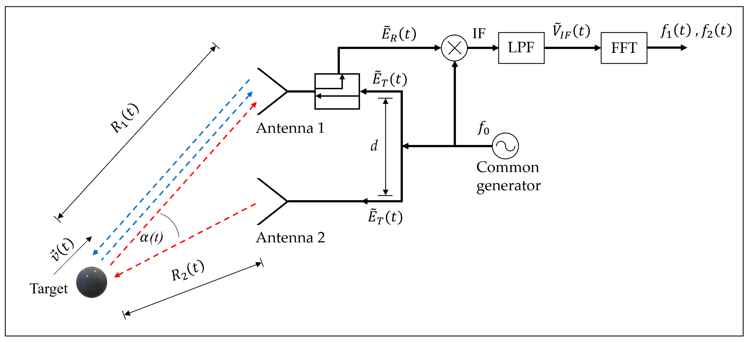
Figure 1 is an illustration of a bi-static radar, consisting of a master transceiver and a slave transmitter, both transmitting a CW waveform at the same carrier frequency. For simplicity, we consider here a situation where the target is moving towards the master antenna (Antenna 1). This is a simplified example, where only the master has the capability of reception of the scattered signal from a ‘threat’ targeting it, while the side antenna (Antenna 2) is illuminating the target at a different observation angle. As will be demonstrated in the upcoming sections, the proposed technique can deal with a general scenario, where the target is moving in an arbitrary direction, by enabling both sites to have the capability of reception of the scattered signal.

The operating principle of a stationary coherent micro-Doppler radar is based on a transmitted signal, ${\tilde{E}}_T\left(t\right)$, which is a CW with amplitude $A_T$ and transmission frequency $f_0$:

$${\tilde{E}}_T\left(t\right)=A_T{e}^{j2\pi f_{0}t}$$

(1)

The transmission is performed by both antennas simultaneously, while the reception is performed by Antenna 1 only. As a result of the multipath between two transmissions and one reception, two transmissions are received by Antenna 1 with different time delays due to the different distances:

$${\tilde{E}}_R\left(t\right)=\left\{A_{R1}exp\left[-j\stackrel{{\theta }_1\left(t\right)}{\overbrace{\frac{2\pi f_0}{c}2R_1\left(t\right) }}\right]+A_{R2}exp\left[-j\stackrel{{\theta }_2\left(t\right)}{\overbrace{\frac{2\pi f_0}{c}\left[R_1\left(t\right)+R_2\left(t\right)\right] }}\right] \right\}\times e^{j2\pi f_{0}t} .$$

(2)

After passing through a mixer and low-pass filter, the following result is obtained:

$${\tilde{V}}_{IF}\left(t\right)={\tilde{E}}_T^{\ast }\left(t\right)\times {\tilde{E}}_R\left(t\right)=A_{R1}{A}_{T}exp\left\{-j{\theta }_1\left(t\right) \right\}+A_{R2}{A}_{T}exp\left\{-j{\theta }_2\left(t\right) \right\} .$$

(3)

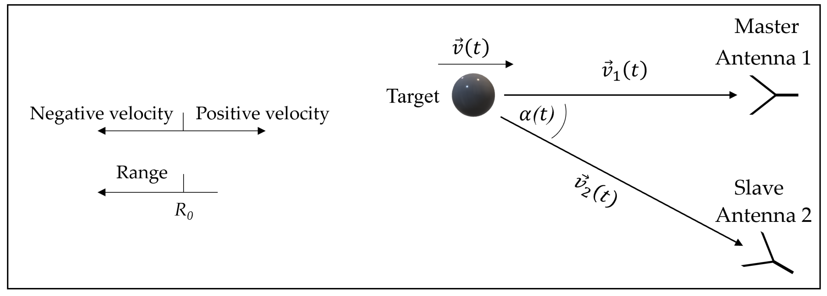
Here, ($·$)* denotes a complex conjugate. There exists a relationship between the two velocity components in the different directions of the transmitters with respect to the angle between the two components, as shown in Figure 2.

The angle $\alpha \left(t\right)$ is the relative observation angle between the two transmitting sites. For the simple scenario described in Figure 2, the respective radial velocity towards each transmitting site is given by:

$$v_1\left(t\right)=v\left(t\right) ,$$

(4)

$$v_2\left(t\right)=v\left(t\right)cos\left({\alpha }_0\right) .$$

(5)

The distances R₁(t) and R₂(t) in Equation (2) are integrals on the relative velocity components, while the direction is given in terms of the instantaneous angle $\alpha \left(t\right)$ between them, with initial location $R_0$ and initial angle ${\alpha }_0$:

$$R_1\left(t\right)=R_0-{\int }_0^t{v}_1\left(t^{\prime }\right)d{t}^{\prime }=R_0-{\int }_0^{t}v\left(t^{\prime }\right)d{t}^{\prime } ,$$

(6)

The distance from Antenna 2 is calculated as follows:

$$R_2\left(t\right)=R_0\times cos\left({\alpha }_0\right)-{\int }_0^t{v}_2\left(t^{\prime }\right)d{t}^{\prime }=R_0\times cos\left({\alpha }_0\right)-{\int }_0^{t}v\left(t^{\prime }\right)cos\left[\alpha \left(t^{\prime }\right)\right]d{t}^{\prime }$$

(7)

From the radar output, ${\tilde{V}}_{IF}\left(t\right)$, in Equation (3), two phases are obtained:

$${\theta }_1\left(t\right)=\frac{2\pi f_0}{c}2R_1\left(t\right)=\frac{2\pi f_0}{c}2 \left[R_0-{\int }_0^{t}v\left(t^{\prime }\right)d{t}^{\prime }\right] ,$$

(8)

$${\theta }_2\left(t\right)=\frac{2\pi f_0}{c}\left[R_1\left(t\right)+R_2\left(t\right)\right]=\frac{2\pi f_0}{c}\left[R_0-{\int }_0^{t}v\left(t^{\prime }\right)d{t}^{\prime }+R_{0}cos\left({\alpha }_0\right)-{\int }_0^{t}v\left(t^{\prime }\right)cos\left[\alpha \left(t^{\prime }\right)\right]d{t}^{\prime }\right] .$$

(9)

Frequency analysis, which is the expected result after FFT, requires a differential on the phases of the radar output ${\tilde{V}}_{IF}\left(t\right)$:

$$f_1\left(t\right)=-\frac{1}{2\pi }\frac{d{\theta }_1\left(t\right)}{dt}=\frac{2f_0}{c}v\left(t\right) ,$$

(10)

$$f_2\left(t\right)=-\frac{1}{2\pi }\frac{d{\theta }_2\left(t\right)}{dt}=\left\{1+cos\left[\alpha \left(t\right)\right]\right\}\underset{\frac{f_1\left(t\right)}{2}}{\underbrace{\frac{f_0}{c}v\left(t\right)}} .$$

(11)

The number of transmitters in the system determines the number of frequencies that are received at the output of the radar. The frequencies will be determined by the velocity components between each transmitter and the target, with the velocity components related to the angles formed between the target and the receiver, and each of the transmitters. In the case of two transmitters, two frequencies will be received at the output of the radar. By using (11), the connection between the two frequencies and the angle between the two transmitters that caused them can be seen in Equation (12):

$$cos\left[\alpha \left(t\right)\right]=2\frac{f_2\left(t\right)}{f_1\left(t\right)}-1 .$$

(12)

Equation (12) presents a way to calculate $\mathsf{\alpha }$ by measuring the frequencies at the radar output. The presented setup describes a simplified model of two transmitters, which causes two different frequencies at the radar output. Such a case might be generalized by increasing the number of transmitters to receive more frequencies, contributing to the detection of more information about the target. We assume in this scheme that there is no need to track a target that does not pose a risk, and therefore we choose to focus on tracking after objects that move directly to one of the transmitters. Regardless of the number of transmitters, there will always be one receiver that has a relatively vertical component in the direction of the target’s motion, more so than the others. In the case of additional transmitters, information according to this model can also be obtained without a vertical component to one of the transmitters. It can be seen from Equation (12) that the instantaneous angle between the two paths plays a role in the resulting ratio between the respective Doppler frequency shifts, while the distances have no direct effect.

3. Range Detection in Super Resolution Using CW Bistatic Radar

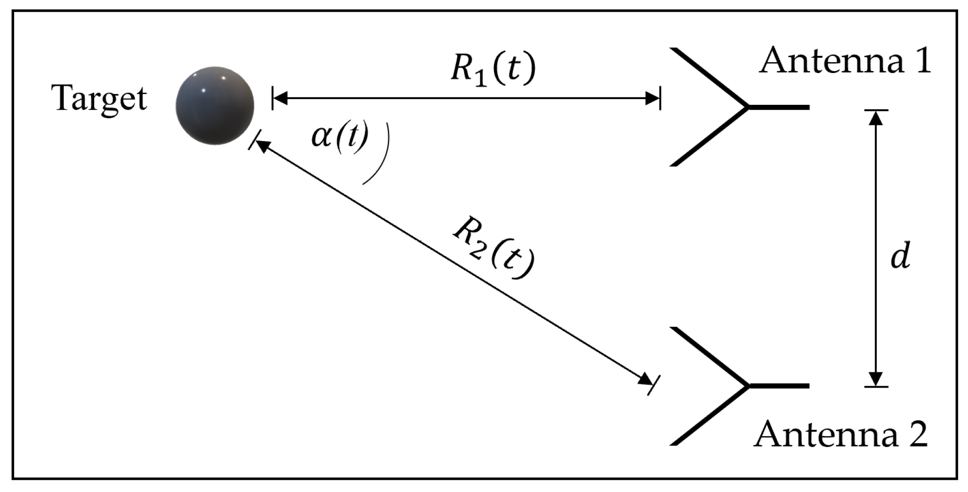
The relationship between the resulted Doppler frequencies and the angle $\alpha \left(t\right)$ between the two directions is now studied. For clarity, we consider a simple scenario where the target moves towards the main antenna, perpendicular to the plane of transmission, as demonstrated Figure 3. We extend the derivation to deal with a more general scenario in the next section. The relation between the distances R₁(t) and R₂(t) and the angle $\alpha \left(t\right)$ are shown in Figure 3.

R₂(t) can be written, by Pythagoras’s law, as follows:

$$R_2\left(t\right)=\sqrt{d^2+{R_1}^2\left(t\right)} .$$

(13)

For triangulation, $\mathit{cos}\left[\alpha \left(t\right)\right]$ can be converted to the following:

$$cos\left[\alpha \left(t\right)\right]=\frac{R_1\left(t\right)}{R_2\left(t\right)}=\frac{R_1\left(t\right)}{\sqrt{d^2+{R_1}^2\left(t\right)}} .$$

(14)

After comparing Equations (12) and (14), the distance $R_1\left(t\right)$ can be written as follows:

$$R_1\left(t\right)=\frac{2\frac{f_2\left(t\right)}{f_1\left(t\right)}-1}{\sqrt{1-{\left(2\frac{f_2\left(t\right)}{f_1\left(t\right)}-1\right)}^2}}\times d .$$

(15)

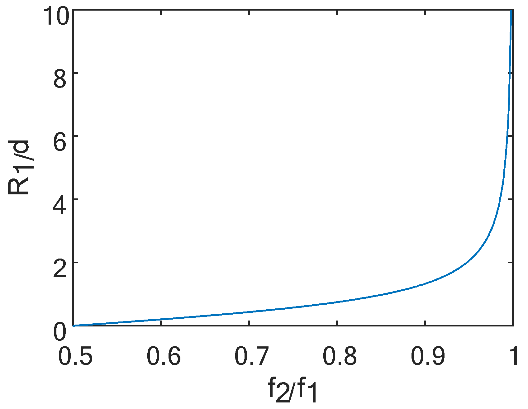
The ratio f₂/f₁ is explained in Figure 4.

From Equations (10) and (11), it can be seen that as $\mathsf{\alpha }$ approaches ${90}^{°}$, when the target is close to antenna 1, the relation between the frequencies f₂/f₁ is equal to 0.5, while Equation (15) and Figure 4 present the same case with distance 0. From Equations (10) and (11), it can be seen that as $\alpha$ approaches $0^{°}$, when the target is far from the radar or the antennas are very close, the relation between the frequencies f₂/f₁ approaches 1. Equation (15) and Figure 4 present the same case when approaching infinity. Equation (15) presents a solution to find the distance of a target from the system without the need for bandwidth, by transmitting a single frequency. By knowing the distance between the transmitters and by analyzing the returns to a single receiver, the target distance can be extracted.

4. Range Detection in the General Scenario

The previous section introduced the simple model for a scenario in which the target moves directly towards the master antenna (Antenna 1) perpendicular to the axis of the transmitters. In the following, we generalize the analysis to consider targets approaching the sensor at an angle β. In such a scenario, the sensor should also detect the direction of target arrival, as illustrated in Figure 5.

It can be seen that Equations (4) and (5) for the simple case of the vertical motion discussed previously are still valid for the general scenario. Therefore, Equation (12) is also relevant here.

In accordance with the cosine theorem, the distance R₂(t) can be expressed in terms of the geometrical quantities:

$$R_2\left(t\right)=\sqrt{R_1^2+d^2-2d{R}_1\left(t\right)\underset{-sin(\beta )}{\underbrace{cos\left(90+\beta \right)}}} .$$

(16)

Similarly, the instantaneous angle $\alpha \left(t\right)$ can be derived from:

$$d^2={R_1}^2\left(t\right)+{R_2}^2\left(t\right)-2R_1\left(t\right)R_2\left(t\right)cos\left[\alpha \left(t\right)\right]$$

(17)

resulting in:

$$cos\left[\alpha \left(t\right)\right]=\frac{R_1{}^2\left(t\right)+{R_2}^2\left(t\right)-d^2}{2R_1\left(t\right)R_2\left(t\right)}$$

(18)

The distance R₂(t) from Equation (16) is now introduced in Equation (18), obtaining:

$$cos\left[\alpha \left(t\right)\right]=\frac{2{R_1}^2\left(t\right)+2d{R}_1\left(t\right)sin\left(\beta \right)}{2R_1\left(t\right)\sqrt{{R_1}^2\left(t\right)+d^2+2d{R}_1\left(t\right)sin\left(\beta \right)}}=\frac{R_1\left(t\right)+dsin\left(\beta \right)}{\sqrt{{R_1}^2\left(t\right)+d^2+2d{R}_1\left(t\right)sin\left(\beta \right)}}$$

(19)

Using Equations (12) and (19), the distance $R_1\left(t\right)$ can be found in terms of the Doppler frequency shifts $f_1\left(t\right)$ and $f_2\left(t\right)$, as obtained at the two respective receivers:

$$2\frac{f_2\left(t\right)}{f_1\left(t\right)}-1=\frac{R_1\left(t\right)+dsin\left(\beta \right)}{\sqrt{{R_1}^2\left(t\right)+d^2+2d{R}_1\left(t\right)sin\left(\beta \right)}}$$

(20)

It can be easily seen that when $\beta =0$, Equation (20) degenerates to the expression given in Equation (15) for the scenario where the target is moving perpendicular to the sensor as discussed in Section 3. The distance $R_1\left(t\right)$ can be found by solving a quadratic equation:

$${R_1}^2\left(t\right)\left[{\left(2\frac{f_2\left(t\right)}{f_1\left(t\right)}-1\right)}^2-1\right]+R_1\left(t\right)2dsin\left(\beta \right)\left[{\left(2\frac{f_2\left(t\right)}{f_1\left(t\right)}-1\right)}^2-1\right]+d^2\left[{\left(2\frac{f_2\left(t\right)}{f_1\left(t\right)}-1\right)}^2-sin{\left(\beta \right)}^2\right]=0$$

(21)

We assume that in most communication and radar systems, the angle of arrival (AoA) of transmission is known, since the use of antenna arrays is very common. When the angle $\mathsf{\beta }$ is known, RDCWB can also be used to track targets in the general scenario. In a scenario when the AoA is unknown, the number of transmitters can be increased so that a situation similar to an antenna array is obtained.

5. Bistatic CW Radar Measurements

A bistatic system was designed, according to Figure 6.

The system was built from a transmitter and a radar that contains a transmitter and a receiver. The system was designed such that the target movement would be in front of the radar and next to the separate transmitter. For these reasons, the separate transmitter was designed to transmit more power than the radar in order to compensate for the wider beam width that was needed to cover the target’s movement. The radar and its parameters are presented in Figure 7.

The system was built as shown in Figure 8.

In the presented experiment, plastic bullets served as targets, as shown in Figure 8. The manufacturer indicates that the bullets are shot at a velocity of 30 m/s. Real bullets move at much higher than 30 m/s velocities, but we chose to perform the measurements on a safer target, even though the same radar has previously performed that successful detection of bullets moving at velocities greater than 1000 m/s. The only difference in measuring bullets at different velocities is the time taken for processing, with low velocities taking longer to process. A fast bullet does not allow long processing times but also does not require it because the high velocity allows less time to be used for processing. Equation (29) demonstrates the relation between the resolution, the velocity, and the processing time. In order to make a comparison between the results of the system and the video recording, it was necessary to perform the measurements on a slow target in relation to the photographic capabilities so that it would be possible to make the comparison. This is another reason we chose to perform measurements on a slow bullet. The measurements were made when bullets were fired from the system and beyond, unlike the developed model, which was for the movement of a target towards the system, because such a measurement was simpler to conduct. Although the experiments were performed when the movement is in the opposite direction, we performed the experiments in order to show the ability to track the range of the bullets, so the direction of movement does not have an impact on the results.

According to Equation (10), it can be seen that higher target velocity results in an increase in the expected Doppler frequency shift. It can be also revealed from Equation (28) that for higher f₁ frequency, an improved resolution is expected. Thus, it is claimed that for a given integration time, a better estimation of the distance and velocity will be achieved for high-speed targets. Noting that in the present laboratory demonstration, relatively slow targets are detected, in common scenarios, where high speed targets are involved, the resulting resolution will be even better.

In addition, in the presented laboratory demonstrations, the targets were made of non-conductive plastic sponge. Such targets present relatively low radar cross section (RCS), while in most scenarios we may expect higher RCS targets. It is important to note that despite their small reflectivity, plastic bullets are shown to be well detected, as can be seen in Figure 9.

A camera and the radar recorded several bullet shots simultaneously. The radar output is analog, and it is necessary to sample it at a frequency that corresponds to the expected maximum velocity of the target. The expected maximum velocity is 30 m/s, and the transmission frequency of the radar is 94 GHz. According to Equation (10), the expected frequency at the radar output is 19 kHz. In order to perform a measurement according to a strict requirement of Nyquist, the sampling frequency was chosen to be 10 times the expected maximum frequency, and therefore, the radar was sampled at f_sample = 200 kHz. The camera was used to present a comparison of the accuracy of the radar measurement after analysis. A spectrogram function was applied to the data from the radar, which split the signal into equal parts and performed a fast Fourier transform on them. The resulting spectrogram was a three-dimensional graph presentation of time, frequency, and intensity, where the frequency and the time are shown in a two-dimensional ordinary graph, and the intensity is represented by colors (as shown in the colormap in Figure 9). A spectrogram is a tool that allows spectral analysis to be displayed over time. The relationship between frequency and velocity in a Doppler radar is linear, so the frequency axis in the spectrogram can easily be replaced by a velocity axis, as shown in the graph of velocity component vectors in Figure 9. The frequency axis is replaced by the velocity axis according to Equation (10) when:

$$v\left[m/s\right]=\frac{c}{2f_0}f=\frac{3\times {10}^8}{2\times 94\times {10}^9}f=0.001595\left[m\right]\times f\left[Hz\right]$$

(22)

The spectrogram was input into an algorithm in order to locate several envelopes on one graph and determine the numeric vectors of each velocity component separately. One velocity vector was obtained from the velocity detected by the transmission from the radar, while the second was obtained from the velocity detected by the transmission from the individual transmitter. Exemplary results of the code and the spectrogram are presented in Figure 9. The spectrogram shown in Figure 9 was created in accordance with the parameters given in

Table 1. Spectrogram parameters from Figure 9.

Spectrogram Parameter	Value
Bullets’ maximum velocity	30 m/s
Expected frequency at radar output	19 kHz
Sampling Frequency	200 kHz
Window in time	10 ms
Window in samples	2048
Zeros Padding factor	$\times$2
Total time for FFT calculation	20 ms
Total samples for FFT calculation	4096 [2048 samples + 2048 zeros padding]
Overlap between windows	99%

.

As the bullet moved away from the radar, the velocity was negative; it had a high negative value at first and decayed with time due to drag from the air. The upper vector in Figure 9 is the result of the transmission from the individual transmitter, and the bottom vector is the result of the radar transmission.

From the presented measurement, it was possible to obtain additional information about the movement direction of the target, based on a comparison between the different velocity components, given the system and the transmitter locations. This type of measurement will become more efficient as the number of transmitters increases.

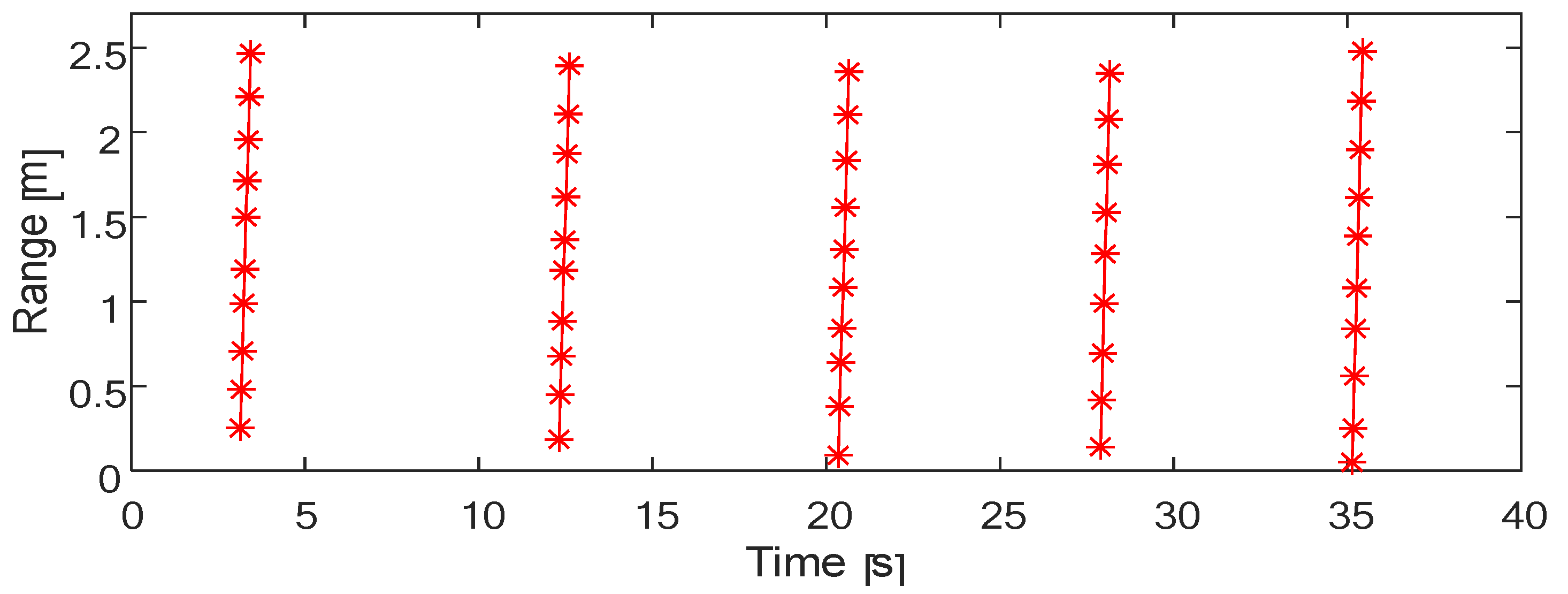
Using the video captured by the camera and a video analysis program, the distance between the radar and the bullet was measured for each frame. The video was recorded according to Figure 6, with the camera filming the movement of the bullet from the side. A known object in the video background helped with the distance normalization; in this case, a TV with known dimensions was captured in the background (Figure 10).

A video recording and recording of the radar were performed for 40 s. During the recording, five shots were fired one after the other. The result is a graph of the bullets’ range over time (Figure 11).

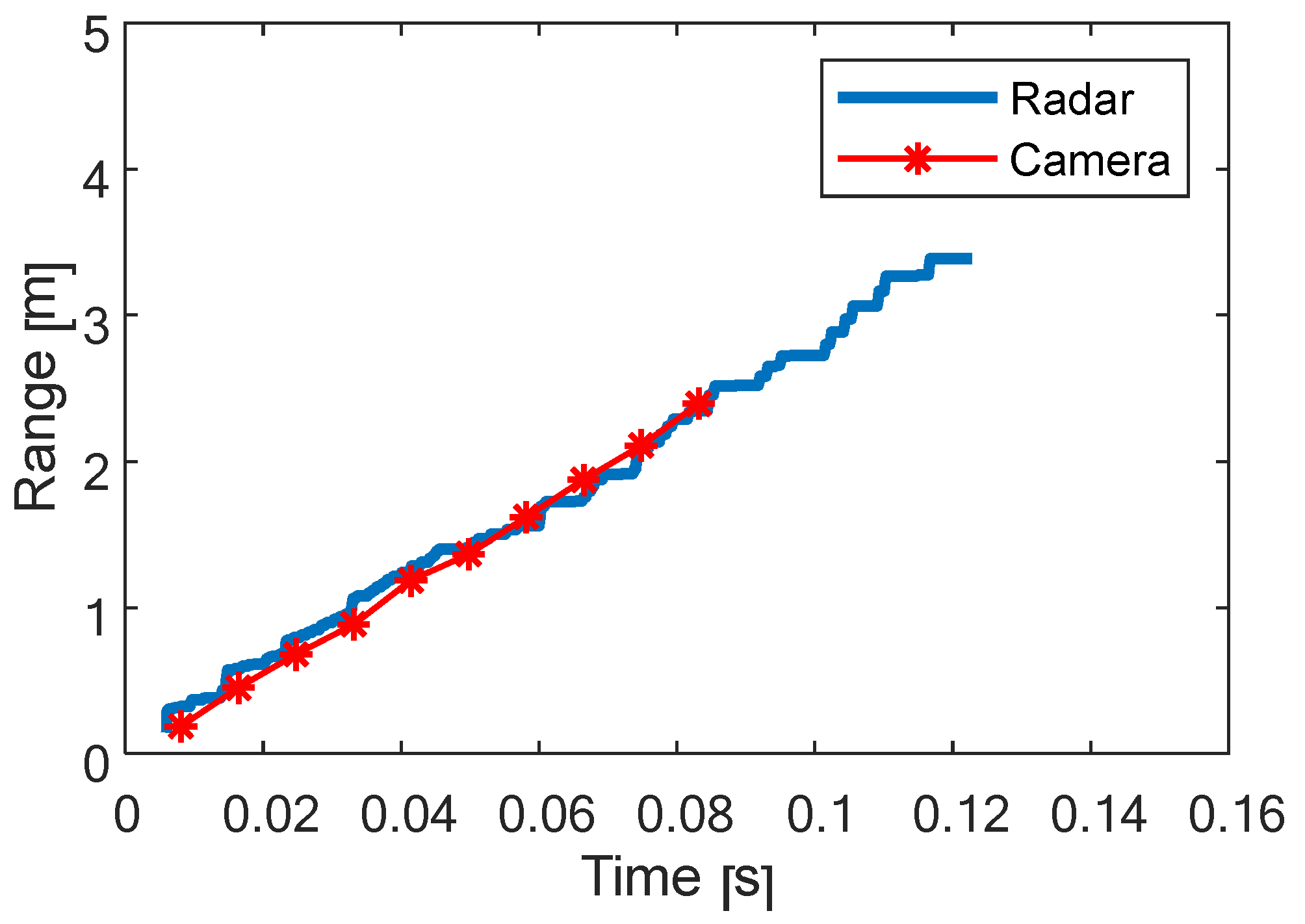
The velocity component vectors of one shot from Figure 9 were inserted to Equation (15) when d = 1.4 m; as a result, a graph was obtained that indicates the position of the bullet relative to the bistatic radar. The video analysis from the camera after the position was determined from the radar is shown in Figure 12, presenting a comparison between the camera and radar, in terms of the accuracy of the radar measurement.

It can be seen that there was an unequivocal match between the camera and radar measurements. According to the measurements, the distance of the moving target can be measured in a non-limited physical resolution, where the distance is greater but at the scale of the distance between the two transmitters. Measurements from both the radar and the camera were inserted into a curve fitting tool, using linear fitting to find the slope and first point in the X-axis with t (R = 0) of both graphs. The estimated values are provided in

Table 2. Slope and start time of shooting comparison between radar and camera.

	Estimated Slope	Estimated Time of Firing Start
Radar	26.5 m/s	0.38 s
Camera	29 m/s	0.4 s

.

There was a less than 10% error between the estimated values from the radar and the camera, as can be seen from the error estimation:

$$Slope Error(\%)=\frac{\left|camer{a}_{est. slope}-rada{r}_{est. slope}\right|}{camer{a}_{est. slope}}\times 100(\%)=8.6\% ,$$

(23)

$$Shooting Time Error(\%)=\frac{\left|camer{a}_{est.time}-rada{r}_{est.time}\right|}{camer{a}_{est. time}}\times 100(\%)=5\% .$$

(24)

6. Bistatic CW Radar Range Resolution Analysis

The range resolution in this method was obtained by a differential on the expression from Equation (15), with x=f₂/f₁:

$$∆R=\frac{dR}{dx}\times ∆x=\frac{2}{{\left[1-{\left(2x-1\right)}^2\right]}^{1.5}}\times d\times ∆x ,$$

(25)

where $∆x$is the error calculation according to $f_1$ and $f_2$:

$$∆x=\sqrt{{\left(\frac{\partial x}{\partial f_2}∆f_2\right)}^2+{\left(\frac{\partial x}{\partial f_1}∆f_1\right)}^2}=\sqrt{{\left(\frac{1}{f_1}∆f_2\right)}^2-{\left(\frac{f_2}{{\left(f_1\right)}^2}∆f_1\right)}^2},$$

(26)

$∆f$is determined according to the sampling frequency over n samples:

$$∆f_1=∆f_2=\frac{f_{sample}}{N}=\frac{1}{T} ,$$

(27)

and T is the time window used for processing from Table 1. Using Equations (25)–(27) will result in $∆R$:

$$∆R=\frac{2}{{\left[1-{\left(2x-1\right)}^2\right]}^{1.5}}\times \frac{\sqrt{1-x^2}}{T\times f_1}\times d ,$$

(28)

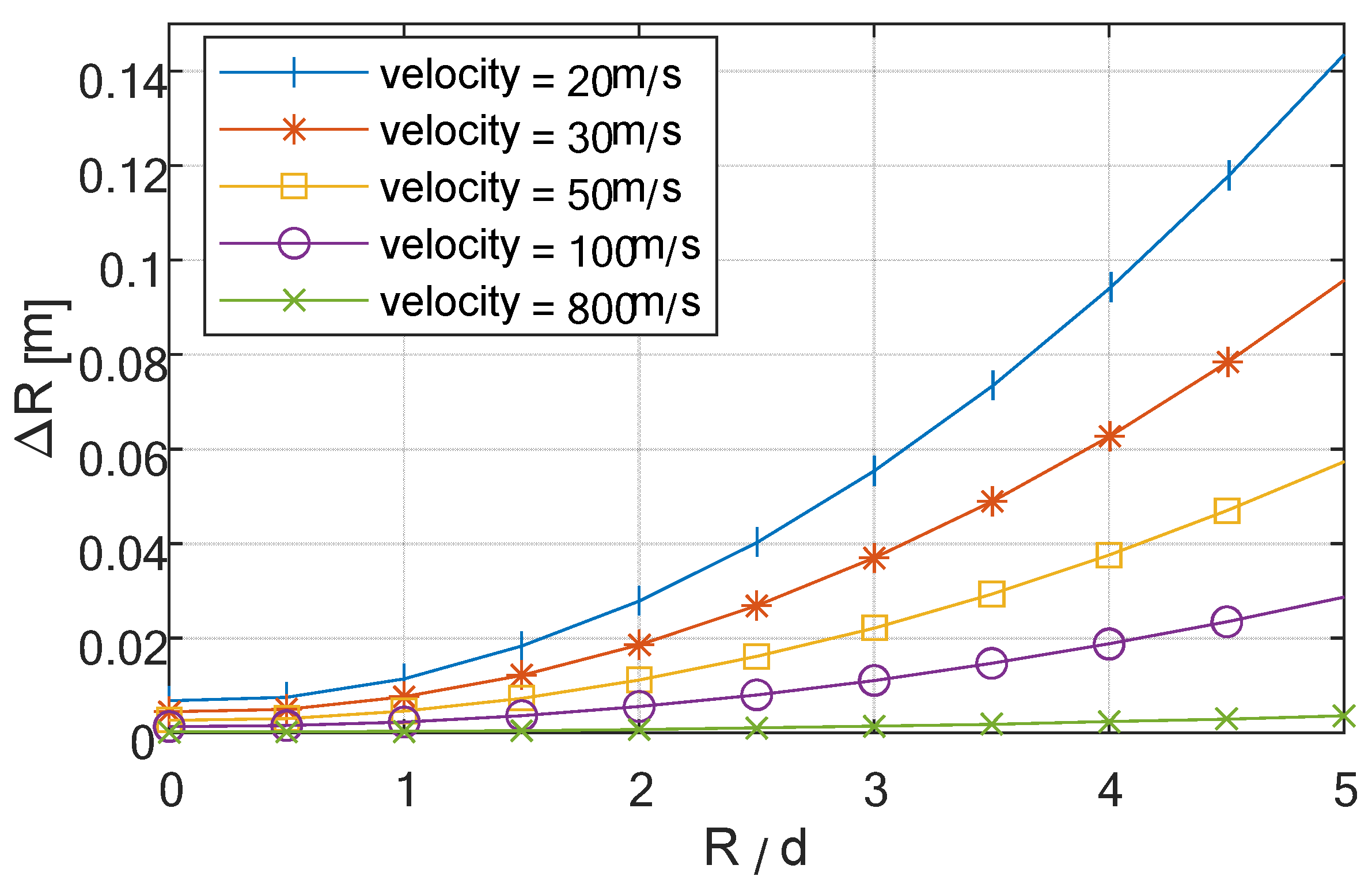
where the variable x depends on the ratio of the frequencies at the radar output, which is determined by the velocity of the target, according to Equations (10) and (11), and the range R between the radar and the target, according to Equation (13) (X-axis in Figure 13). For that reason, $∆R$ from Equation (28) (Y-axis in Figure 13) can be determined as a function of the velocity, range R, and distance d from Equation (15), as shown in the graph in Figure 13. The parameter T was selected as 20 ms in order to create Figure 12, providing a clear observation of the target (Figure 13).

Figure 13 shows how the relationship between the desired range for detection and the size, d, of the system influences the range resolution. When the ratio between R and d is ideal, the range resolution that can be obtained is less than 2 cm; meanwhile, when the ratio is 1, the range resolution is less than 1 cm.

7. Barrier for Range Resolution in RDCWB

A low barrier can be set for the distance resolution from Equation (28). The low barrier is obtained when the distance approaches 0, so it can be stated that x = 0.5 according to Equation (15) and Figure 4. The frequency $f_1$ is replaced by Equation (10), so the low barrier can be written as:

$${∆R|}_{x=0.5}\ge 2.6\times {10}^8\times \frac{d}{f_0\times T\times v}$$

(29)

From Equation (29), it can be concluded that four main parameters influence the resolution of the proposed scheme.

7.1. Integration Time and Velocity

The barrier is determined by the integration time for the FFT calculation and by the velocity of the target, while the transmitted frequency $f_0$ is fixed throughout the measurement. Since a large integration time can be compensated by a greater percentage of overlap between windows for FFT calculation, it can be said that the integration time is the significant parameter that affects the resolution. As long as the processing capabilities are stronger, the possible integration time is bigger, and the range resolution improves.

7.2. Transmission Frequency

It can be seen that determining transmission frequency sets the barrier in Equation (29). Other than larger scattering strength at high frequency (as mentioned in the introduction), increasing the transmission frequency also lowers the barrier in the proposed scheme and improves the range resolution. In addition, it can be seen from Equation (10) that a high transmission frequency causes a higher frequency at the radar output. In order to detect the frequency at the radar output an FFT operation should be performed on the signal. A high frequency signal requires less recording time to detect its power spectrum density. Therefore, it can be said that given a target with a defined velocity, it will be detected faster when the transmission frequency is higher. There is no limit to the velocity that can be detected. At any transmission frequency it will be theoretically possible to detect any velocity; the limit is usually in the system itself.

7.3. Distance between the Transmitters

According to Equation (29), enlarging the distance d between the two transmitters spoils the resolution and raises the barrier from Equation (29) but increases the effective distance for detection, as can be seen in Figure 9, where the ability to separate the different frequencies obtained at the radar output depends on the ratio between the distance of the target and the distance between the two transmitters. It can be seen from Equation (11) that a larger alpha angle causes a larger difference between the frequencies.

8. The Effect of Noise on Tracking Accuracy

The signal-to-noise ratio obtained at the IF affects the precision of targets tracking [27]. In order to examine the effect of SNR on the tracking accuracy of target location, an additive white Gaussian noise (AWGN) n(t) is introduced in the received signal in (2). The signal with the noise is given by:

$$E_R\left(t\right)+n\left(t\right)=\left[A_{R1}\hspace{0.17em}{e}^{-j{\theta }_1\left(t\right)}+A_{R2}\hspace{0.17em}{e}^{-j{\theta }_2\left(t\right)}\right]e^{j2\pi f_{0}t}+n\left(t\right)$$

(30)

For convenience, we assume from now on that both scattered signals are received with the same power, i.e., $A_{R1}=A_{R2}=A_R$. The noise is presented using quadrature base-band components:

$$n\left(t\right)=\left[n_I\left(t\right)+j{n}_Q\left(t\right)\right]e^{j2\pi f_{0}t}$$

(31)

Here, $n_I$ and $n_Q$ are independent, Gaussian stochastic processes, with zero statistical average $\overline{n_I\left(t\right)}=\overline{n_Q\left(t\right)}=0$ and variance $\overline{n_I^2\left(t\right)}=\overline{n_Q^2\left(t\right)}={\sigma }_n^2$, equal to the noise power. Introducing the noise into the heterodyning detection results in:

$$V_{IF}\left(t\right)=A_T{A}_R{e}^{-j{\theta }_1\left(t\right)+\Delta \theta \left(t\right)}+\hspace{0.17em}{A}_T{A}_R{e}^{-j{\theta }_2\left(t\right)+\Delta \theta \left(t\right)}$$

(32)

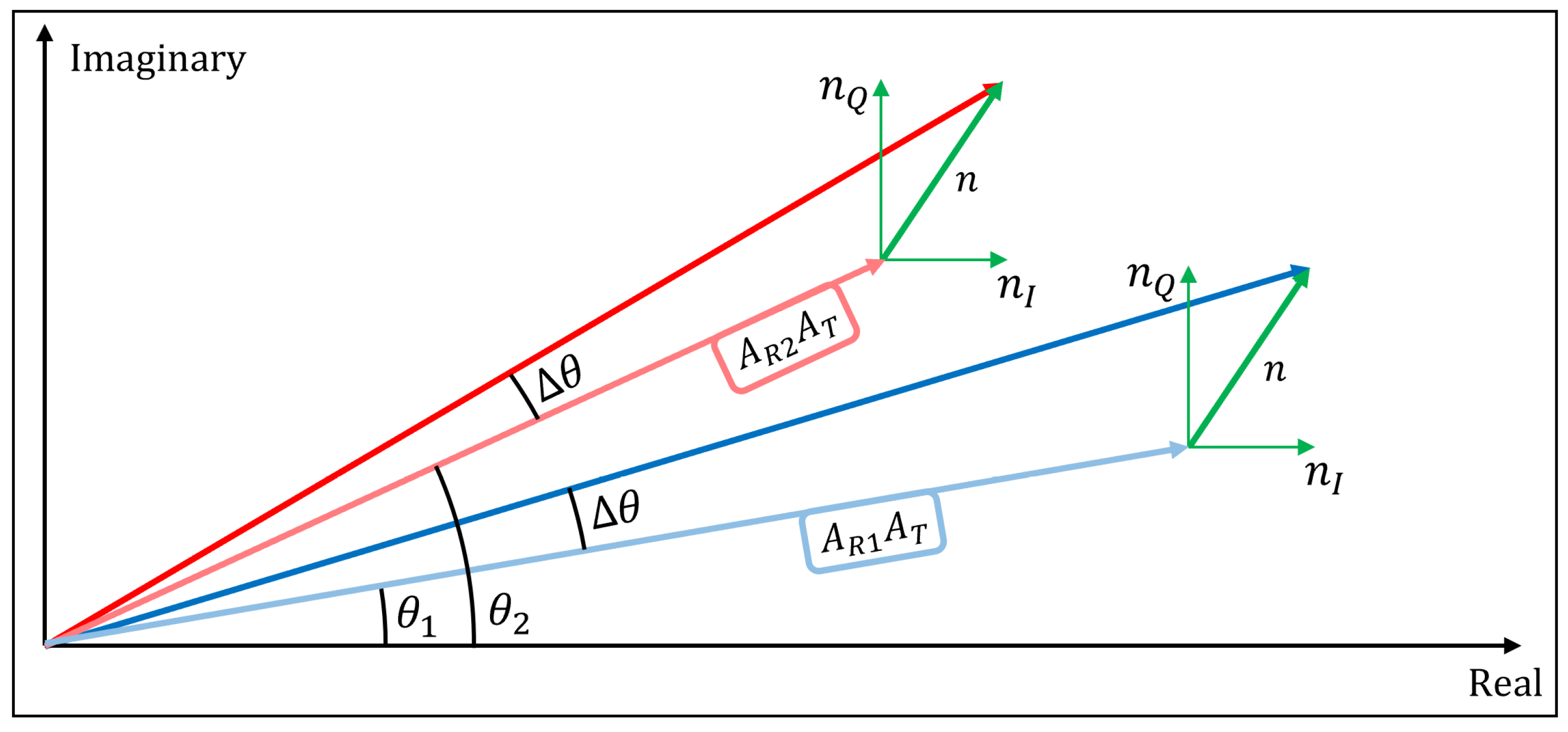
where the phase noise fluctuations of the two products obtained at the mixer output can be expressed as:

$$\Delta \theta \left(t\right)=arctg\left[\frac{n_Q\left(t\right)}{A_R+n_I\left(t\right)}\right]$$

(33)

The phasor description of the detected signals in the presence of AWGN is depicted in Figure 14. The common analytical derivation of phase noise in angle (phase or frequency) modulated waveforms considers the case where the reception is above the threshold, i.e., $A_R\gg n_I\left(t\right),n_Q\left(t\right)$. In this case:

$$\Delta \theta \left(t\right)=arctg\left[\frac{n_Q\left(t\right)}{A_R+n_I\left(t\right)}\right]\cong arctg\left[\frac{n_Q\left(t\right)}{A_R}\right]\cong \frac{n_Q\left(t\right)}{A_R}$$

(34)

The phase fluctuations cause frequency modulation (FM) in the Doppler shifts, leading to a spectral spread. The phase noise is shown to be a gaussian process with zero mean $\overline{∆\theta \left(t\right)}=0$ and variance $∆{\theta }_{RMS}^2\left(t\right)=\overline{∆{\theta }^2\left(t\right)}={\sigma }_n^2/A_R^2$. The corresponding FM fluctuations is given in terms of the phase derivative:

$$\Delta \nu \left(t\right)=\frac{1}{2\pi }\frac{d}{dt}\Delta \theta \left(t\right)=\frac{1}{2\pi A_R}\frac{d}{dt}{n}_Q\left(t\right)$$

(35)

We use the notation $∆\nu \left(t\right)$ to distinguish the frequency broadening caused by the noise from the frequency resolution $∆f=1/T$ determined by the temporal windowing (integration time). The FM noise is also Gaussian with mean $\overline{∆\nu \left(t\right)}=0$. The power spectral density (PSD) of the frequency fluctuations is used to derive the expression for its variance $∆{\nu }_{RMS}^2$:

$$S_{\Delta \nu }\left(f\right)=\frac{1}{{A_R}^2}{f}^2{S}_{n_Q}\left(f\right)\to \Delta {\nu }_{RMS}^2={\displaystyle \underset{-\infty }{\overset{+\infty }{\int }}{S}_{\Delta \nu }\left(f\right)df}=\frac{1}{{A_R}^2}{\displaystyle \underset{-\infty }{\overset{+\infty }{\int }}{f}^2{S}_{n_Q}\left(f\right)df}$$

(36)

where $S_{n_Q}\left(f\right)={\sigma }_n^2/B$ is the PSD of the noise. Considering the noise-equivalent bandwidth of B, the variances of the FM noise of the detected signals are found to be:

$$\Delta {\nu }_{RMS}^2=\frac{1}{{A_R}^2}{\displaystyle \underset{-B}{\overset{+B}{\int }}{f}^2{S}_{n_Q}\left(f\right)df}=\frac{2}{3}{B}^2\frac{{\sigma }_n^2}{{A_R}^2}=\frac{1}{3}{B}^2\frac{1}{SNR}$$

(37)

where the signal-to-noise ratio is $SNR=A_R^2/\left(2{\sigma }_n^2\right)$.

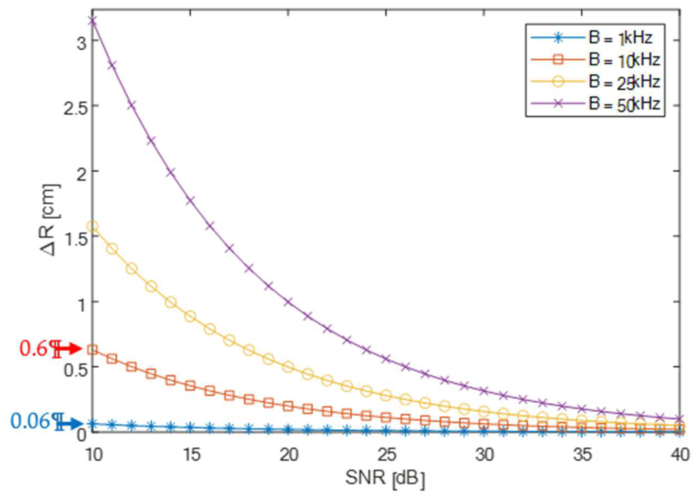
Substituting $∆f_1=∆f_2=∆{\nu }_{RMS}$ from (37) into Equations (25) and (26), the graph of the range accuracy $∆R$ as a function of the signal-to-noise ratio (SNR) for different bandwidths is presented in Figure 15.

Note that for the examined bandwidths, increasing the SNR results in range tracking accuracy approaches the range resolution determined by the integration time.

9. The Proposed RDCWB Scheme vs. Other Range Detection Sensors

Measurements were carried out using plastic bullets in order to prove the method. If the measurement is performed on a real bullet, which moves at a velocity of 800 m per second, and R/d = 5, the range resolution in the proposed method will be, according to Equations (10) and (11):

$$f_1=\frac{2f_0}{c}v=\frac{2\times 94\times {10}^9}{3\times {10}^8}800=501.33 kHz$$

(38)

$$f_2=\left\{1+cos\left[\alpha \left(t\right)\right]\right\}\frac{f_1}{2}=\left\{1+cos\left[ta{n}^{-1}\left(\frac{d}{R}\right)\right]\right\}\frac{f_1}{2}=1.9806\times \frac{501330}{2}=496.46 kHz$$

(39)

The obtained range resolution is 3.7 cm, according to Equation (28) and the frequencies from Equations (38) and (39), where d = 1 m and the processing time is 2 ms (shorter due to the higher velocity). Standard systems (FMCW Radar or Pulse Radar) for range detection with a range resolution of 3.7 cm must perform transmission and reception in ultra-wideband, according to:

$$BW=\frac{c}{2\times ∆R}=4 GHz$$

(40)

where BW is the required bandwidth, c is the speed of light, and $∆R$ is the range resolution. Developing a system with this requirement is expensive, and it is very difficult to implement, whereas the method proposed in this study does not require such high bandwidth.

The pros and cons of each system type can be summarized. Existing range detection sensors have range resolution which depends on the bandwidth of the system. There are systems that can detect a range with a resolution of a few centimeters, although they require a bandwidth of several GHz. There is an advantage in favor of existing systems whose range resolution does not depend on the target distance from the system.

In the proposed RDCWB in this study, there is a disadvantage that the range resolution depends on the distance of the target from the system, but it can be compensated by spacing between the locations of the transmitters. The significant advantage of the proposed system is the resolution of several cm, which is easily achieved in an easy-to-implement system that does not transmit with bandwidth but a single transmission frequency.

10. Further Applications and Discussion

The experiments performed in this study were performed in a non-neutral environment. There were many objects in the room, and the room was not electromagnetically isolated. From this can be deduced the great advantage of using a Doppler system, which is immune to interference, although it can be blocked. However, it cannot be manipulated to sense fake targets because the system is only coherent to itself. Therefore, the proposed scheme can be used for the purposes of identifying tiny movements, for situations where existing systems have difficulty performing, such as identifying the breathing of survivors under rubble. The rubble does not constitute a radar clatter, as long as there is a tiny movement of breathing or limb movement. A system similar to the proposed RDCWB can direct rescue forces toward survivors.

Recently, the field of intelligent reflective surface (IRS) has been extensively researched [28,29]. These surfaces have been found to be efficient and even significantly increase the range in communication networks through non-line-of-sight paths between the transmitter and the receiver. This method can be imported into the proposed scheme in this study, where the scattering of reflective surfaces in the area of the proposed RDCWB can contribute significantly to an increase in the effective distance for detection and possibly also to an improvement in range resolution, even when the target is significantly far away from the transmitters.

In recent years, there has been a significant development in using artificial intelligence for high resolution tracking of targets, with an emphasis on artificial neural networks (ANN) processing [30,31]. It is possible that the proposed scheme of RDCWB can take a further significant step with the help of ANN techniques.

Figure 13 presents the disadvantage of the system, when the resolution is not useful as the target is far from the system. For many systems such as vehicle radars or missile and bullet protection systems, this disadvantage is insignificant, as it is often not necessary to know the exact range when the target is far away. The necessity for accurate range is more significant when the target is closer to the system.

11. Summary and Conclusions

Bistatic radar is, in most cases, more effective than monostatic radar in the detection of evasive targets. In addition to this capability, a method was developed for the indirect measurement of range. This method enabled the radar to provide information on the range of a target as well as on the target’s velocity and direction.

Measurements were made using bullets with low RCS, small size, and a structure that usually does not disperse in the radar direction. Measurements of firing were made in parallel with a camera, and a comparison was made between the results obtained by processing the radar and video analysis. The comparison showed the ability to detect the target’s range at very high resolution with an error of less than 10%. The expected range resolution in the measurement, which was designed and performed according to the optimal parameters of the system and the bullets, was between 0.4 and 5 cm. Measurements were performed on plastic bullets with low velocity, whereas real bullets with higher velocity can be measured at a range resolution of 3 cm under the same system parameters.

The proposed method utilized a minimum number of transmitters. With the generalization of this setup using multiple transmitters, additional results and capabilities could be obtained in order to discover more information about targets, such as their relative angle to the radar.

References

- Wenger, J.; Hahn, S. Long Range and Ultra-Wideband Short Range Automotive Radar. In Proceedings of the 2007 IEEE International Conference on Ultra-Wideband, Singapore, 24–26 September 2007; pp. 518–522. [Google Scholar] [CrossRef]
- Molchanov, P.; Gupta, S.; Kim, K.; Pulli, K. Short-range FMCW monopulse radar for hand-gesture sensing. In Proceedings of the 2015 IEEE Radar Conference (RadarCon), Arlington, VA, USA, 10–15 May 2015; pp. 1491–1496. [Google Scholar] [CrossRef]
- Balal, Y.; Balal, N.; Richter, Y.; Pinhasi, Y. Time-Frequency Spectral Signature of Limb Movements and Height Estimation Using Micro-Doppler Millimeter-Wave Radar. Sensors 2020, 20, 4660. [Google Scholar] [CrossRef] [PubMed]
- Akiyama, I.; Yoshizumi, N.; Ohya, A.; Aoki, Y.; Matsuno, F. Search for Survivors Buried in Rubble by Rescue Radar with Array Antennas—Extraction of Respiratory Fluctuation. In Proceedings of the 2007 IEEE International Workshop on Safety, Security and Rescue Robotics, Rome, Italy, 27–29 September 2007; pp. 1–6. [Google Scholar] [CrossRef]
- Arai, I. Survivor search radar system for persons trapped under earthquake rubble. In Proceedings of the APMC 2001—2001 Asia-Pacific Microwave Conference (Cat. No.01TH8577), Taipei, Taiwan, 3–6 November 2001; Volume 2, pp. 663–668. [Google Scholar] [CrossRef]
- Liang, X.; Lv, T.; Zhang, H.; Gao, Y.; Fang, G. Through-wall human being detection using UWB impulse radar. J. Wireless Com. Netw. 2018, 2018, 46. [Google Scholar] [CrossRef] [Green Version]
- Wang, X.; Xu, L.; Sun, H.; Xin, J.; Zheng, N. On-Road Vehicle Detection and Tracking Using MMW Radar and Monovision Fusion. IEEE Trans. Intell. Transp. Syst. 2016, 17, 2075–2084. [Google Scholar] [CrossRef]
- Kramer, J. An integrated optical transient sensor. IEEE Trans. Circuits Syst. II Analog Digit. Signal Process. 2002, 49, 612–628. [Google Scholar] [CrossRef]
- Blunt, S.D.; Gerlach, K.; Higgins, T. Aspects of Radar Range Super-Resolution. In Proceedings of the 2007 IEEE Radar Conference, Waltham, MA, USA, 17–20 April 2007; pp. 683–687. [Google Scholar] [CrossRef]
- Westra, A.G. Radar Versus Stealth: Passive Radar and the Future of U.S. Military Power; National Defense Univ Washington DC Inst For National Strategic Studies: Washington, DC, USA, 2009. [Google Scholar]
- Dungan, K.E.; Austin, C.; Nehrbass, J.; Potter, L.C. Civilian vehicle radar data domes. In Algorithms for Synthetic Aperture Radar Imagery XVII; International Society for Optics and Photonics: Bellingham, WA, USA, 2010. [Google Scholar]
- Li, Z.; Chen, H.; Duan, S.; Bi, Y.; Lei, H.; Lai, Y.; Wu, H.; Li, D. Reflectivity calibration for X-band solid-state radar with metal sphere. In Proceedings of the 2016 IEEE International Geoscience and Remote Sensing Symposium (IGARSS), Beijing, China, 10–15 July 2016; pp. 4765–4768. [Google Scholar]
- Balal, N.; Balal, Y.; Richter, Y.; Pinhasi, Y. Detection of Low RCS Supersonic Flying Targets with a High-Resolution MMW Radar. Sensors 2020, 20, 3284. [Google Scholar] [CrossRef] [PubMed]
- Hülsmann, A.; Zech, C.; Klenner, M.; Tessmann, A.; Leuther, A.; Lopez-Diaz, D.; Schlechtweg, M.; Ambacher, O. Radar system components to detect small and fast objects. Terahertz Phys. Devices Syst. IX Adv. Appl. Ind. Def. 2015, 9483, 1–10. [Google Scholar] [CrossRef]
- Balal, N.; Richter, Y.; Pinhasi, Y. Identifying low-RCS targets using micro-Doppler high-resolution radar in the millimeter waves. In Proceedings of the 2020 14th European Conference on Antennas and Propagation (EuCAP), Copenhagen, Denmark, 15–20 March 2020; pp. 1–5. [Google Scholar] [CrossRef]
- Arish, K.S.; Yong-Hoon, K. Automatic Measurement of Blade Length and Rotation Rate of Drone Using W-Band Micro-Doppler Radar. IEEE Sens. J. 2018, 18, 1895–1902. [Google Scholar]
- Caris, M.; Johannes, W.; Sieger, S.; Port, V.; Stanko, S. Detection of Small UAS with W-band Radar. In Proceedings of the 2017 18th International Radar Symposium (IRS), Fraunhoferstr, Germany, 28–30 June 2017. [Google Scholar]
- Chang, E.; Sturdivant, R.L.; Quilici, B.S.; Patigler, E.W. Micro and Mini Drone Classification Based on Coherent Radar Imaging. In Proceedings of the 2018 IEEE Radio and Wireless Symposium (RWS), Anaheim, CA, USA, 15–18 January 2018. [Google Scholar]
- Ritchie, M.; Fioranelli, F.; Griffiths, H.; Torvik, B. Monostatic and bistatic radar measurements of birds and micro-drone. In Proceedings of the 2016 IEEE Radar Conference, Philadelphia, PA, USA, 2–6 May 2016. [Google Scholar]
- Miler, A.W.; Clemente, C.; Robinson, A.; Greig, D.; Kinghorn, A.M.; Soraghan, J.J. Micro-Doppler based target classification using multi-feature integration. In Proceedings of the IET Intelligent Signal Processing Conference 2013, London, UK, 2–3 December 2013. [Google Scholar]
- Youngwook, K.; Hao, L. Human Activity Classification Based on Micro-Doppler Signature Using a Support Vector Machine. IEEE Trans. Geosci. Remote Sens. 2009, 47, 1328–1337. [Google Scholar] [CrossRef]
- Kulpa, K.S.; Misiurewicz, J. Stretch Processing for Long Integration Time Passive Covert Radar. In Proceedings of the 2006 CIE International Conference on Radar, Shanghai, China, 16–19 October 2006. [Google Scholar]
- Bezoušek, P.; Schejbal, V. Bistatic and Multistatic Radar Systems. Radioengineering 2008, 17, 53–59. [Google Scholar]
- O’Hagan, D.W.; Capria, A.; Petri, D.; Kubica, V.; Greco, M.; Berizzi, F.; Stove, A.G. Passive Bistatic Radar (PBR) for harbour protection applications. In Proceedings of the 2012 IEEE Radar Conference, Atlanta, GA, USA, 7–11 May 2012. [Google Scholar]
- Aydin, K.; Walsh, T.M. Millimeter Wave Scattering from Spatial and Planar Bullet Rosettes. IEEE Trans. Geosci. Remote Sens. 1999, 37, 1138–1150. [Google Scholar] [CrossRef]
- Winkler, V. Range Doppler detection for automotive FMCW radars. In Proceedings of the 2007 European Radar Conference, Munich, Germany, 10–12 October 2007; pp. 166–169. [Google Scholar] [CrossRef]
- Droitcour, A.D.; Boric-Lubecke, O.; Kovacs, G.T.A. Signal-to-Noise Ratio in Doppler Radar System for Heart and Respiratory Rate Measurements. IEEE Trans. Microw. Theory Tech. 2009, 57, 2498–2507. [Google Scholar] [CrossRef]
- Kudathanthirige, D.; Gunasinghe, D.; Amarasuriya, G. Performance Analysis of Intelligent Reflective Surfaces for Wireless Communication. In Proceedings of the ICC 2020—2020 IEEE International Conference on Communications (ICC), Dublin, Ireland, 7–11 June 2020; pp. 1–6. [Google Scholar] [CrossRef]
- Pérez-Adán, D.; Fresnedo, Ó.; González-Coma, J.P.; Castedo, L. Intelligent Reflective Surfaces for Wireless Networks: An Overview of Applications, Approached Issues, and Open Problems. Electronics 2021, 10, 2345. [Google Scholar] [CrossRef]
- Kuter, S.; Akyurek, Z.; Weber, G.W. Retrieval of fractional snow covered area from MODIS data by multivariate adaptive regression splines. Remote Sens. Environ. 2018, 205, 236–252. Available online: https://www.sciencedirect.com/science/article/pii/S0034425717305709 (accessed on 1 December 2021). [CrossRef]
- Derr, K.; Manic, M. Wireless based object tracking based on neural networks. In Proceedings of the 2008 3rd IEEE Conference on Industrial Electronics and Applications, Singapore, 3–5 June 2008; pp. 308–313. [Google Scholar] [CrossRef]