A Semianalytical Algorithm for Estimating Water Transparency in Different Optical Water Types from MERIS Data

Abstract

Water transparency (or Secchi disk depth:$Z_{SD}$) is a key parameter of water quality; thus, it is very important to routinely monitor. In this study, we made four efforts to improve a state-of-the-art $Z_{SD}$ estimation algorithm that was developed in 2019 on the basis of a new underwater visibility theory proposed in 2015. The four efforts were: (1) classifying all water into clear (Type I), moderately turbid (Type II), highly turbid (Type III), or extremely turbid (Type IV) water types; (2) selecting different reference wavelengths and corresponding semianalytical models for each water type; (3) employing an estimation model to represent reasonable shapes for particulate backscattering coefficients based on the water type classification; and (4) constraining likely wavelength range at which the minimum diffuse attenuation coefficient (K_d(λ)) will occur for each water type. The performance of the proposed $Z_{SD}$ estimation algorithm was compared to that of the original state-of-the-art algorithm using a simulated dataset (N = 91,287, $Z_{SD}$ values 0.01 to 44.68 m) and an in situ measured dataset (N = 305, $Z_{SD}$ values 0.3 to 16.4 m). The results showed a significant improvement with a reduced mean absolute percentage error (MAPE) from 116% to 65% for simulated data and from 32% to 27% for in situ data. Outliers in the previous algorithm were well addressed in the new algorithm. We further evaluated the developed $Z_{SD}$ estimation algorithm using medium resolution imaging spectrometer (MERIS) images acquired from Lake Kasumigaura, Japan. The results obtained from 19 matchups revealed that the estimated $Z_{SD}$ matched well with the in situ measured $Z_{SD}$, with a MAPE of 15%. The developed $Z_{SD}$ estimation algorithm can probably be applied to different optical water types due to its semianalytical features.

1. Introduction

Water transparency relates to the depth to which light will penetrate water and to photosynthesis changes in a specific waterbody over time; thus, it is key to thoroughly evaluating water quality [1,2,3,4,5,6,7,8,9]. Changes in water transparency can also be an indicator of a human threat to an ecosystem [10,11,12,13,14]. Water transparency is often represented using Secchi disk depth ($Z_{SD}$), which can be measured using a traditional Secchi disk or estimated using the remote sensing technique. Recently, the remote sensing technique has been widely used because it is capable of providing a synoptic view of $Z_{SD}$ distribution in waters and estimation algorithms have been fine tuned [15,16,17].

Generally, two types of $Z_{SD}$ estimation algorithms are used with the remote sensing technique: empirical and semianalytical algorithms. Empirical algorithms use a simple regression analysis between remote sensing data and in situ measured $Z_{SD}$ values, while semianalytical algorithms are based on an underwater visibility theory [4,18,19,20,21]. Compared to empirical algorithms, they are more suitable for estimating $Z_{SD}$ values from remote sensing data because they can be applied to various waters without the requirements of in situ data for algorithm recalibration [21,22].

Two underwater visibility theories are currently in use: the classic theory proposed in 1952 [23] and the new theory proposed in 2015 [4]. Previous studies have found that $Z_{SD}$ estimation algorithms based on the new theory perform better than those based on the classic theory [4,20,21,22,24]. Algorithms based on the new theory rely on the diffuse attenuation coefficient (K_d(λ)) at a wavelength corresponding to the maximum light transparency [4]. In these algorithms, the accurate estimation of total absorption and backscattering coefficients (a$\left(\lambda \right)$ and b_b(λ), respectively) using an appropriate quasianalytical algorithm (QAA) is a key step for estimating $Z_{SD}$ values more accurately. Therefore, the selection of the most appropriate QAA for each water type is necessary [4,15,19,21,25,26,27,28].

Recently, Jiang et al. [21] developed a semianalytical algorithm (hereafter referred to as the Jiang19 algorithm) to estimate $Z_{SD}$ values with the aim of improving a $Z_{SD}$ estimation algorithm developed previously by Lee et al. [4]. Both algorithms are based on the new underwater visibility theory. However, only two water types (i.e., clear and turbid waters) were considered in the Jiang19 algorithm, and thus only two reference wavelengths (560 nm for clear waters and 754 nm for turbid water) were used to estimate a$\left(\lambda \right)$ and b_b(λ). Although previous studies have confirmed the success of using 560 nm for clear waters [29] and 754 nm for highly turbid waters [30] as reference wavelengths in total absorption coefficient estimations, the assumption of a pure water absorption coefficient dominating the total absorption coefficient at these two wavelengths will probably be invalid in moderately turbid and extremely turbid waters. This is because the absorption coefficients of phytoplankton and nonalgal particles at 560 and 754 nm will also be high in moderately and extremely turbid waters [31]. Therefore, the applicability of the Jiang19 algorithm to different optical water types is still a challenge. It is thus necessary to revisit the Jiang19 algorithm and improve its water type classification, reference wavelength selection, and water-type-corresponding QAA application to estimate more accurate $Z_{SD}$ values in waters with different optical properties.

Consequently, the objectives of our study were to: (1) develop a new algorithm for estimating $Z_{SD}$ more accurately in waters with different optical properties by classifying more water types and by selecting a more appropriate reference wavelength and corresponding QAA for each water type; and (2) evaluate the performance of the developed $Z_{SD}$ estimation algorithm using synthetic, in situ, and medium resolution imaging spectrometer (MERIS) data.

2. Materials and Methods

2.1. Data Acquisition

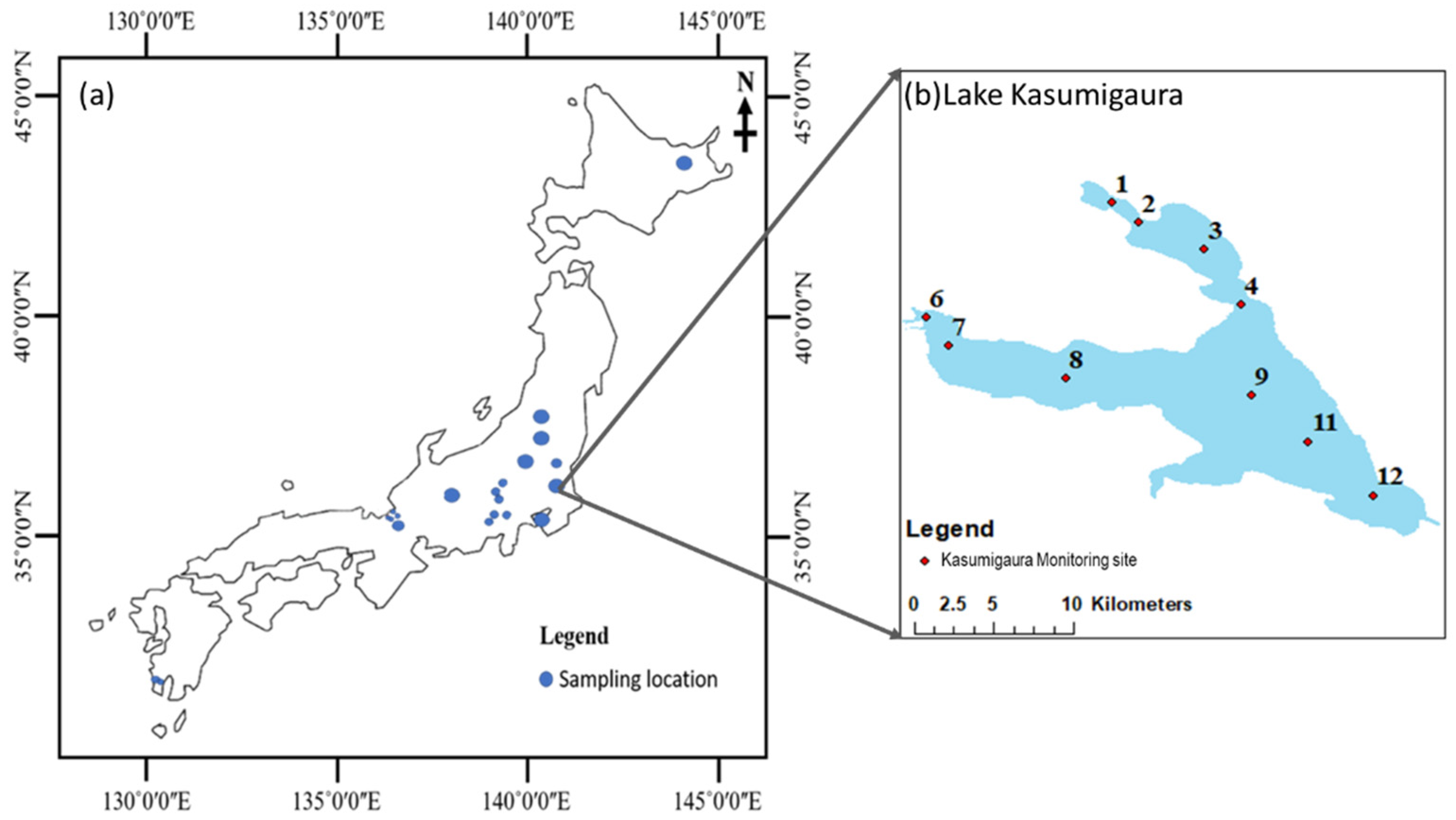
2.1.1. In Situ Data Collection

We collected 305 in situ measured hyperspectral remote sensing reflectance ($R_{rs}$(λ)) and $Z_{SD}$ data pairs from 20 lakes and Tokyo Bay in Japan (Figure 1, hereafter referred to as the in situ dataset). The $Z_{SD}$ values were measured with a 30 cm diameter white Secchi disk. The $Z_{SD}$ data ranged from 0.3 to 16.4 m and covered clear to highly turbid waters. The in situ measured $R_{rs}$(λ) values were obtained through the above-water approach. This approach measures the radiance of the skylight (L_s), the total upwelling radiance from the water (L_t), and the radiance from a standard gray board (L_g) using a FieldSpec^® HandHeld spectroradiometer (ASD, Boulder, CO, USA) with a sensor zenith angle of 40° and an azimuth angle of 135° from the sun [32]. All measurements were carried out between 9:30 to 14:00 local time (three measurements were taken between 14:00 and 16:00). Then, the $R_{rs}$ was calculated as follows:

$$R_{rs}=\left(L_t-\rho L_s\right)/\left(\frac{\pi }{R_g}{L}_g\right)-\Delta$$

(1)

where $\rho$ is the water surface reflectance factor (0.028 when the wind speed is less than 5 m/s) [32], R_g is the reflectance of the gray board, and $\Delta$ is the residual reflected skylight calculated using a method proposed by Jiang et al. [33]. All $R_{rs}$(λ) spectra were then converted to MERIS bands based on the MERIS spectral response functions. This dataset was used to evaluate the performance of the developed $Z_{SD}$ estimation algorithm.

To further evaluate the estimated $Z_{SD}$ values from MERIS images, we also acquired in situ measured $Z_{SD}$ values at 10 stations in Lake Kasumigaura (Figure 1b) between January 2003 and March 2012 from the Lake Kasumigaura database, which were collected by the National Institute for Environmental Studies (NIES), Japan [34].

2.1.2. Synthetic Data Collection and Generation

In this study, we collected one synthetic dataset from Jiang et al. [31], which is called Synthetic Dataset I (N = 91,287) in

Table 1. Summary of Synthetic Datasets I, II, and III.

Synthetic Dataset	I (Jiang et al. [31])	II (This Study)	III (This Study)	Total Number of Data	Usage
Parameter	$a\left(\lambda \right)$$, b_b\left(\lambda \right)$$, R_{rs}\left(\lambda \right)$	$K_d\left(\lambda \right)$	$Z_{SD}$(0.01–44.68 m)	91,287	Algorithm Validation

. Synthetic Dataset I contains pairs of $R_{rs}$(λ) spectra as well as total absorption coefficient (a$\left(\lambda \right)$) and total backscattering coefficient (b_b(λ)) values. The $R_{rs}$(λ) spectra were generated from the simulated a$\left(\lambda \right)$ and b_b(λ) values by using a bio-optical model proposed by Gordon et al. [35] and Lee et al. [29] with assumptions of a nadir viewing angle and optically deep waters. For Synthetic Dataset I, the chlorophyll-a concentration (C_chl), tripton concentration (C_tr), and CDOM absorption coefficient at 440 nm (a_CDOM(440)) were varied with different intervals between 0.01–1000 mg/m³, 0.01–1000 g/m³, and 0.01–5 m⁻¹, respectively. More details on Synthetic Dataset I generation can be found in Jiang et al. [31].

We then generated two other synthetic datasets to help with the development and evaluation of the algorithms. Synthetic Dataset II contains the diffuse attenuation coefficient (K_d(λ)) values, which were generated from the simulated a$\left(\lambda \right)$ and b_b(λ) values in Synthetic Dataset I by using the following semianalytical equation proposed by Lee et al. [36,37]:

$$K_d\left(\lambda \right)=\left(1+0.005\theta \right)a\left(\lambda \right)+4.259(1-0.265{\eta }_w\left(\lambda \right)\left(1-0.52e^{-10.8a\left(\lambda \right)}\right)b_b\left(\lambda \right)$$

(2)

where θ is the solar zenith angle and ${\eta }_w$is the ratio of $b_{bw}$ (backscattering coefficient of pure water [38]) to $b_b$.

Synthetic Dataset III consists of simulated $Z_{SD}$ values. These $Z_{SD}$ values were generated from the simulated K_d(λ) values (Synthetic Dataset II) and the corresponding $R_{rs}$(λ) values (Synthetic Dataset I) using the following semianalytical equation developed by Jiang et al. [21]:

$$Z_{SD}=\frac{1}{\left(1+K_T/K_d\right)·\min K_d\left(\lambda \right)}\ln \left(\frac{\left|0.14-R_{rs}^{PC}\right|}{C_t^r}\right), K_T/K_d=\frac{1.04{\left(1+5.4\mu \right)}^{0.5}}{1/{\left(1-\frac{sin{\left(\theta \right)}^2}{R{I}^2}\right)}^{0.5}}$$

(3)

where min $K_d\left(\lambda \right)$ is the minimum $K_d\left(\lambda \right)$ value among the visible wavelengths, $R_{rs}^{PC}$is the corresponding $R_{rs}$ at the wavelength with the minimum $K_d\left(\lambda \right)$, $C_t^r$ is the contrast threshold for sighting a white disk (i.e., 0.013 sr⁻¹), RI is the refractive index value of water (1.34, [39]), $K_T$ is the diffuse attenuation coefficient of upwelling radiance at the wavelength with the minimum $K_d\left(\lambda \right)$, $\theta$ is the solar zenith angle, and $\mu$ is defined as b_b/(a+b_b). A summary of all synthetic datasets is listed in Table 1.

2.1.3. Satellite Data Collection and Processing

In our study, the MERIS Level-1B data between 2002 and 2012 for Lake Kasumigaura were collected from the European Space Agency (ESA, https://merisfrs-merci-ds.eo.esa.int, accessed on 4 February 2018). We selected MERIS data due to their good spatial (300 × 300 m) and spectral (15 bands in visible and near-infrared domains) characteristics. Atmospheric correction was performed using the Case-2 Regional Processor in BEAM 5.0, and clouds and cloud shadows were identified using the IdePix module in SNAP. We then masked out the pixels with clouds, cloud buffers, cloud shadows, and failed atmospheric correction. Finally, we compiled 19 matchups from Lake Kasumigaura by matching the acquisition times of in situ measured $Z_{SD}$ values and satellite images (acquired on the same day). These matchups were used to further evaluate the performance of the developed $Z_{SD}$ estimation algorithm. In addition, the averages of the $Z_{SD}$ values derived from 3-by-3 pixels were used as satellite-estimated values.

2.2. Development of a $Z_{SD}$ Estimation Algorithm

2.2.1. The Original Jiang19 Algorithm

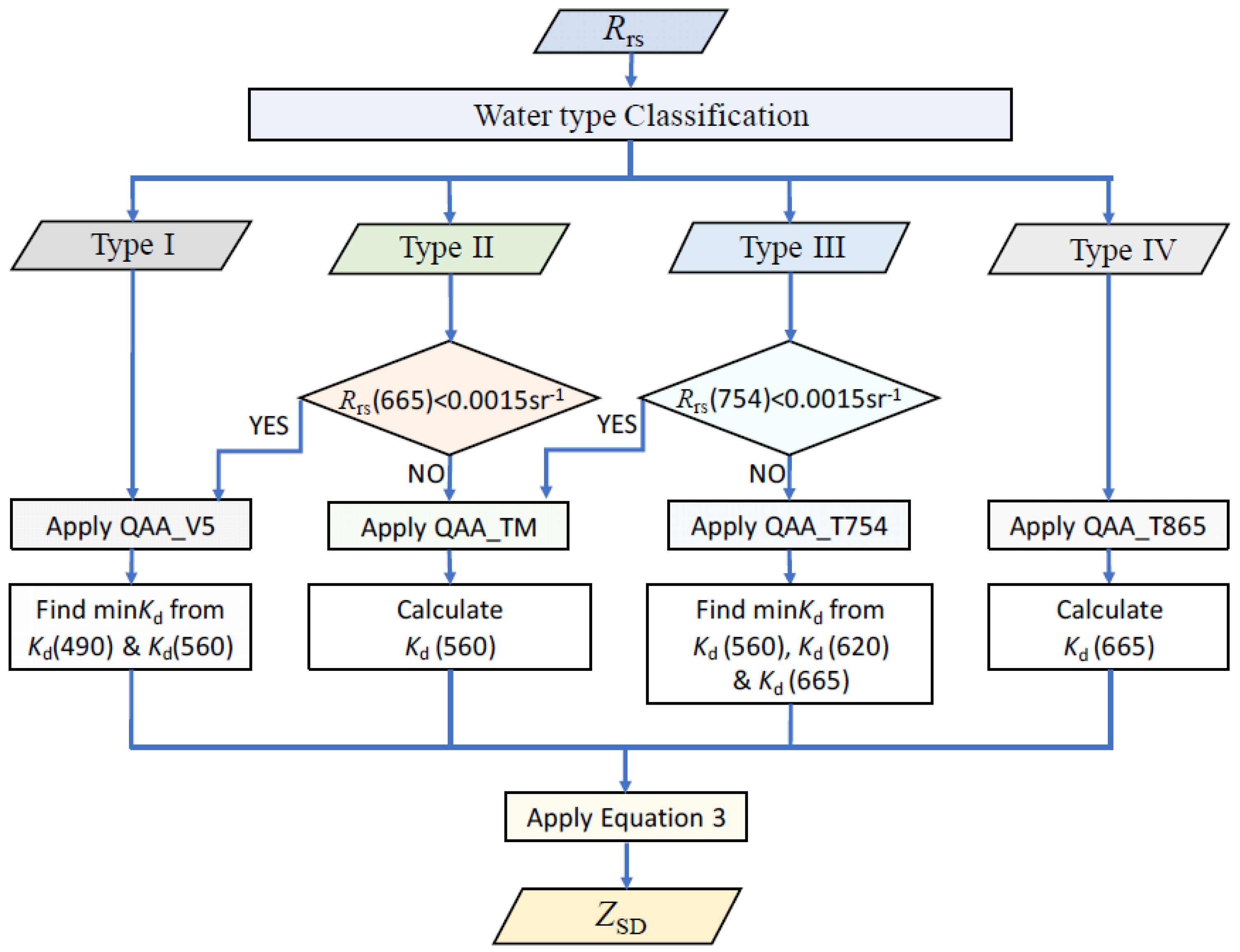
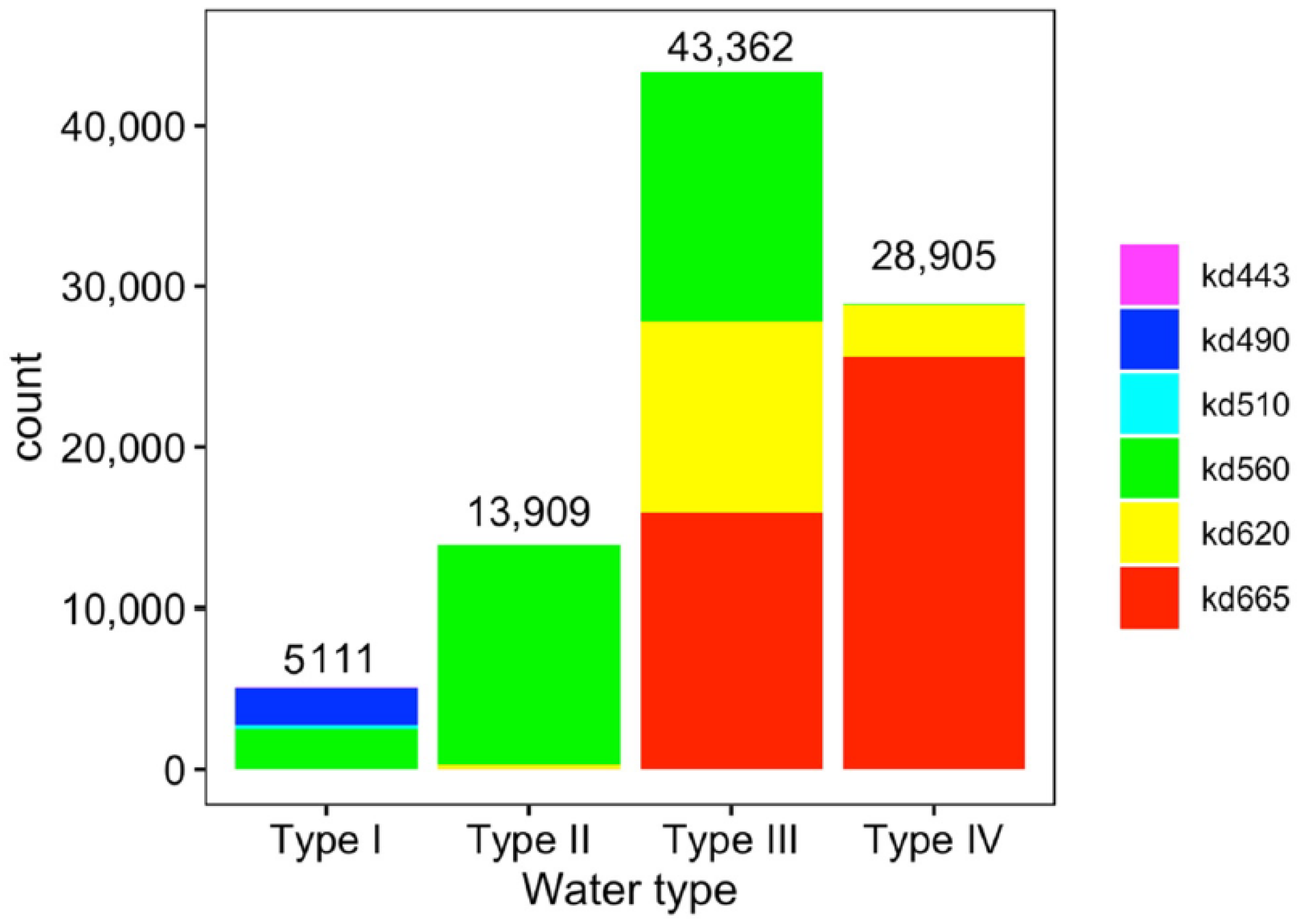
The original Jiang19 algorithm contains three main steps. First, a QAA hybrid is developed to retrieve $a\left(\lambda \right)$ and $b_b\left(\lambda \right)$ from $R_{rs}$(λ) spectra. In the QAA hybrid, a maximum chlorophyll index (MCI) proposed by Gower et al. [40] is used to switch QAA_V5 [29] and QAA_T (i.e., QAA_Turbid in [30]). In detail, if MCI <= 0.0016 sr⁻¹, 560 nm is used as the reference wavelength and thus QAA_V5 is selected to estimate $a\left(\lambda \right)$ and $b_b\left(\lambda \right)$ for clear waters; otherwise, 754 nm is used as the reference wavelength and thus QAA_T is selected to estimate $a\left(\lambda \right)$ and $b_b\left(\lambda \right)$ for turbid waters.

Then, $K_d\left(\lambda \right)$ is estimated from $a\left(\lambda \right)$and $b_b\left(\lambda \right)$ using Equation (2) as the second step, and $Z_{SD}$ is estimated from the minimum $K_d\left(\lambda \right)$ in the visible domain (e.g., 443 nm, 490 nm, 510 nm, 560 nm, 620 nm, 665 nm) and the corresponding $R_{rs}$(λ) using Equation (3) (the third step).

2.2.2. Development of a New $Z_{SD}$ Estimation Algorithm

Since previous studies have confirmed that semianalytical Equations (2) and (3) are robust in waters with different optical properties if accurate $a\left(\lambda \right)$ and $b_b\left(\lambda \right)$ are provided (e.g., [4,21,22,36,41]), our efforts were focused on how to obtain more accurate $a\left(\lambda \right)$ and $b_b\left(\lambda \right)$ values from $R_{rs}$(λ) spectra. A flowchart of the developed $Z_{SD}$ estimation algorithm is shown in Figure 2. Comparing to the Jiang19 algorithm, four improvements were carried out in this study, which are detailed sequentially in the following paragraphs.

First, we adopted a recently proposed water type classification algorithm that can classify all waters into four types, clear (Type I), moderately turbid (Type II), highly turbid (Type III), and extremely turbid (Type IV), by comparing the values of $R_{rs}$ at 490, 560, 620, and 754 nm [31]. This approach allowed us to more reasonably assume that the pure water absorption coefficient dominated the total absorption coefficients at the reference wavelengths (i.e., 560 nm for Types I & II, 754 nm for Type III, and 865 nm for Type IV) [29,31,42]. The water type classification algorithm is described as follows:

$$\begin{array}{l}\mathrm{If} R_{rs}\left(490\right) > R_{rs}\left(560\right), \mathrm{then} \mathrm{Type} \mathrm{I} \mathrm{waters},\hfill \\ \mathrm{Else}, \mathrm{if} R_{rs}\left(490\right) > R_{rs}\left(620\right), \mathrm{then} \mathrm{Type} \mathrm{II} \mathrm{waters},\hfill \\ \mathrm{Else}, \mathrm{if} R_{rs}\left(754\right) > R_{rs}\left(490\right) \mathrm{and} R_{rs}\left(754\right) > 0.01 {\mathrm{sr}}^{-1}, \mathrm{then} \mathrm{Type} \mathrm{IV} \mathrm{waters},\hfill \\ \mathrm{Else}, \mathrm{Type} \mathrm{III} \mathrm{waters}.\hfill \end{array}$$

(4)

Second, we selected a different reference wavelength and corresponding QAA for each water type to retrieve $a\left({\lambda }_0\right)$ and $b_b\left({\lambda }_0\right)$ values at the reference wavelength (${\lambda }_0$). For Type I waters, we selected 560 nm as the reference wavelength and then used an empirical equation in QAA_V5 to estimate a(560) due to its good performance in clear water [29,43,44,45]. The Equations are:

$$a\left(560\right)=a_w\left(560\right)+{10}^{-1.146-1.366x-0.469x^2}$$

(5)

$$x={log}_{10}(\frac{r_{rs}\left(443\right)+r_{rs}\left(490\right)}{r_{rs}\left(560\right)+5\frac{r_{rs}\left(665\right)}{r_{rs}\left(490\right)}{r}_{rs}\left(665\right)})$$

(6)

where $r_{rs}$ is the remote sensing reflectance just below the water surface, a_w(560) is the absorption coefficient of pure water at 560 nm, and $a\left(560\right)$ is the total absorption coefficient at 560 nm.

For Type II waters, we selected the same wavelength (i.e., 560 nm) as the reference wavelength but used a different empirical equation from QAA_TM (developed by Curtarelli et al. [42]) to estimate a(560). We adopted QAA_TM because of its good performance in moderately turbid waters compared to QAA_V6 developed by Lee et al. [42,46]. The equation is:

$$a\left(560\right)=a_w\left(560\right)+0.43{(\frac{R_{rs}\left(560\right)}{R_{rs}\left(665\right)+R_{rs}\left(709\right)})}^{-1.44}$$

(7)

where $R_{rs}\left(560\right)$, $R_{rs}\left(665\right)$, and $R_{rs}\left(709\right)$ are the remote sensing reflectance just above the water surface at 560, 665, and 709 nm, respectively. However, since Equation (7) used a longer wavelength (709 nm) than those used in Equation (6), and considering the effects of a low signal-to-noise ratio in a practical application, we followed Lee et al.’s [46] suggestion to use QAA_V5 for the waters with $R_{rs}$(665) < 0.0015 sr⁻¹ (i.e., we still used Equations (5) and (6)).

For Type III waters, 754 nm was selected as the reference wavelength, and the equations from QAA_T were adopted to estimate a(754) (i.e., $a\left(754\right)\approx a_w\left(754\right)$ [30]). Similar to the consideration for Type II waters, we used a threshold of $R_{rs}$(754) < 0.0015 sr⁻¹ and used QAA_TM for those waters with lower $R_{rs}$(754). This approach allowed us to avoid the effects of a low signal-to-noise ratio in a practical application.

For Type IV waters, 865 nm was selected as the reference wavelength and the assumption of a(865) ≈ $a_w$(865) was adopted, as suggested by Jiang et al. [31]. After estimation of a(${\lambda }_0$) at the reference wavelength (${\lambda }_0$), the particulate backscattering coefficient ($b_{bp}\left({\lambda }_0\right))$could be calculated by the following equation [21,29]:

$$b_{bp}\left({\lambda }_0\right)=\frac{\mu \left({\lambda }_0\right)a\left({\lambda }_0\right)}{1-\mu \left({\lambda }_0\right)}-b_{bw}\left({\lambda }_0\right)$$

(8)

Here, b_bw(λ₀) is the backscattering coefficient of pure water at the reference wavelength.

In the third effort, we employed two empirical models (for Types I and II, respectively) and one semianalytical model (for both Types III and IV waters), which can represent reasonable shapes for particulate backscattering coefficients (b_bp(λ)), thereby allowing us to retrieve more accurate a$\left(\lambda \right)$ and b_b(λ) values at a given wavelength for each water type. For Type I waters, the spectral slope $Y$ was calculated using an empirical Equation in Lee et al. [29]:

$$Y=2.0\left(1-1.2exp\left(-0.9\frac{r_{rs}\left(443\right)}{r_{rs}\left(560\right)}\right)\right)$$

(9)

For Type II waters, the spectral slope $Y$ was calculated using a different empirical Equation in Curtarelli et al. [42]:

$$Y=0.5248exp\left(\frac{r_{rs}\left(665\right)}{r_{rs}\left(709\right)}\right)$$

(10)

For Types III and IV waters, the spectral slope $Y$ was calculated using a semianalytical Equation in Yang et al. [30]:

$$Y=-372.99{\left[{log}_{10}\left(\frac{\mu \left(754\right)}{\mu \left(779\right)}\right)\right]}^2+37.286{log}_{10}\left(\frac{\mu \left(754\right)}{\mu \left(779\right)}\right)+0.84$$

(11)

Then $a\left(\lambda \right)$ and b_b(λ) at the given wavelength (λ) were calculated using the following Equations [29]:

$$b_b\left(\lambda \right)=b_{bw}\left(\lambda \right)+b_{bp}\left({\lambda }_0\right){(\frac{{\lambda }_0}{\lambda })}^Y$$

(12)

$$a\left(\lambda \right)=\frac{\left(1-\mu \left(\lambda \right)\right)b_b\left(\lambda \right)}{\mu \left(\lambda \right)}$$

(13)

To summarize the second and third efforts, we selected QAA_V5 for Type I waters, QAA_TM for Type II waters, QAA_T with a reference wavelength of 754 nm (hereafter renamed QAA_T754) for Type III waters, and QAA_T with a reference wavelength of 865 nm (renamed QAA_T865) for Type IV waters.

In the fourth effort, we carried out a statistical analysis using Synthetic Dataset II to investigate the possibility of a minimum K_d(λ) for each water type. Figure 3 shows the number of synthetic water samples with the minimum K_d(λ) occurring at each visible wavelength for each water type. From the figure, we can observe that the minimum K_d(λ) almost always occurred at 490 and 560 nm for Type I waters, 560 nm for Type II waters, 560, 620, and 665 nm for Type III waters, and at 665 nm for Type IV waters. Accordingly, we considered the relating wavelengths to find the minimum K_d(λ) for each water type. This effort avoided the selection of inappropriate wavelengths due to estimation errors in the previous steps (e.g., due to uncertainty in the estimations of Y values using Equations (9)–(11).

2.3. Accuracy Assessment

We used the root mean square error (RMSE) in a $lo{g}_{10}$ unit, the mean absolute percentage error (MAPE), bias, and the Nash-Sutcliffe efficiency (NSE) to evaluate the performance of the developed algorithm. The Equations are as follows:

$$\mathrm{RMSE}=\sqrt{\frac{{{\displaystyle \sum }}_{i=1}^N{\left[{log}_{10}\left(X_{estimated,i}\right)-{log}_{10}\left(X_{measured,i}\right)\right]}^2}{N}}$$

(14)

$$\mathrm{MAPE}=\frac{1}{N}{\displaystyle \sum }_{i=1}^N\left|\frac{X_{estimated,i}-X_{measured,i}}{X_{measured,i}}\right|·100\%$$

(15)

$$\mathrm{Bias}={10}^Y-1,\hspace{1em}\hspace{1em}Y=\frac{{{\displaystyle \sum }}_{i=1}^N\left[{log}_{10}\left(X_{estimated,i}\right)-{log}_{10}\left(X_{measured,i}\right)\right]}{N}$$

(16)

$$\mathrm{NSE} =1-\frac{{{\displaystyle \sum }}_{i=1}^N{\left(X_{estimated,i}-X_{measured,i}\right)}^2}{{{\displaystyle \sum }}_{i=1}^N{\left(X_{measured,i}-\overline{X_{measured}}\right)}^2}$$

(17)

where $X_{estimated}$ is the estimated $Z_{SD}$ value, $X_{measured}$ is the corresponding in situ measured or known $Z_{SD}$ value, $\overline{X_{measured}}$ is the mean of in situ measured or known $Z_{SD}$ values, and N is the number of data pairs. The regression results between the estimated and the known or in situ measured $Z_{SD}$ values (i.e., R², slope, and intercept) were also used to help evaluate algorithm performance.

3. Results

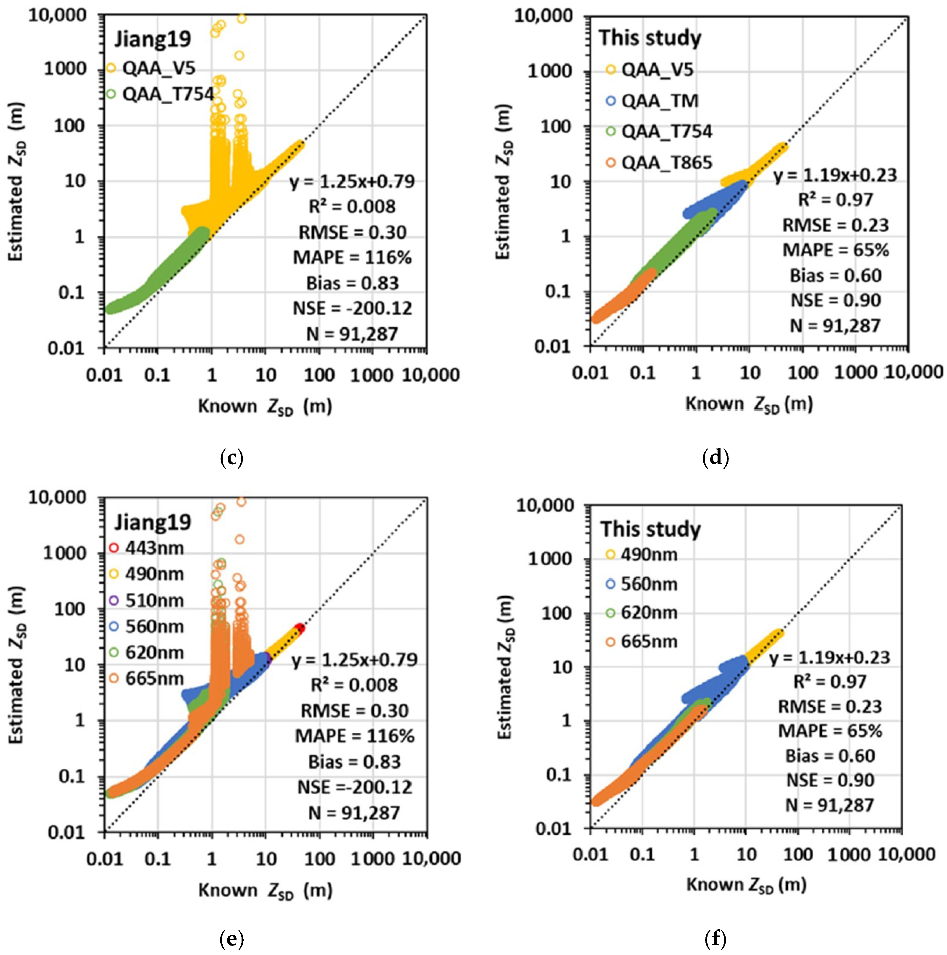
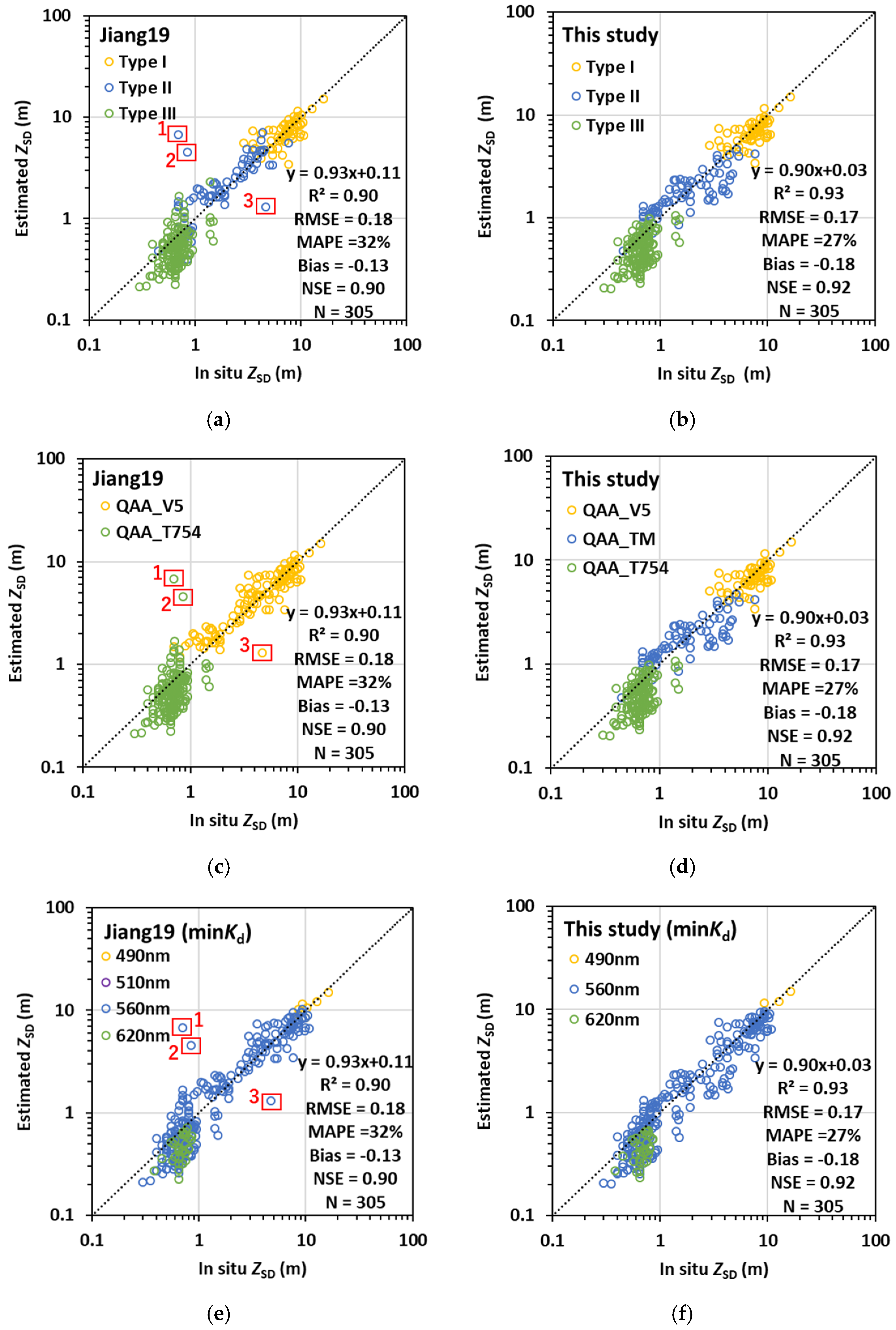
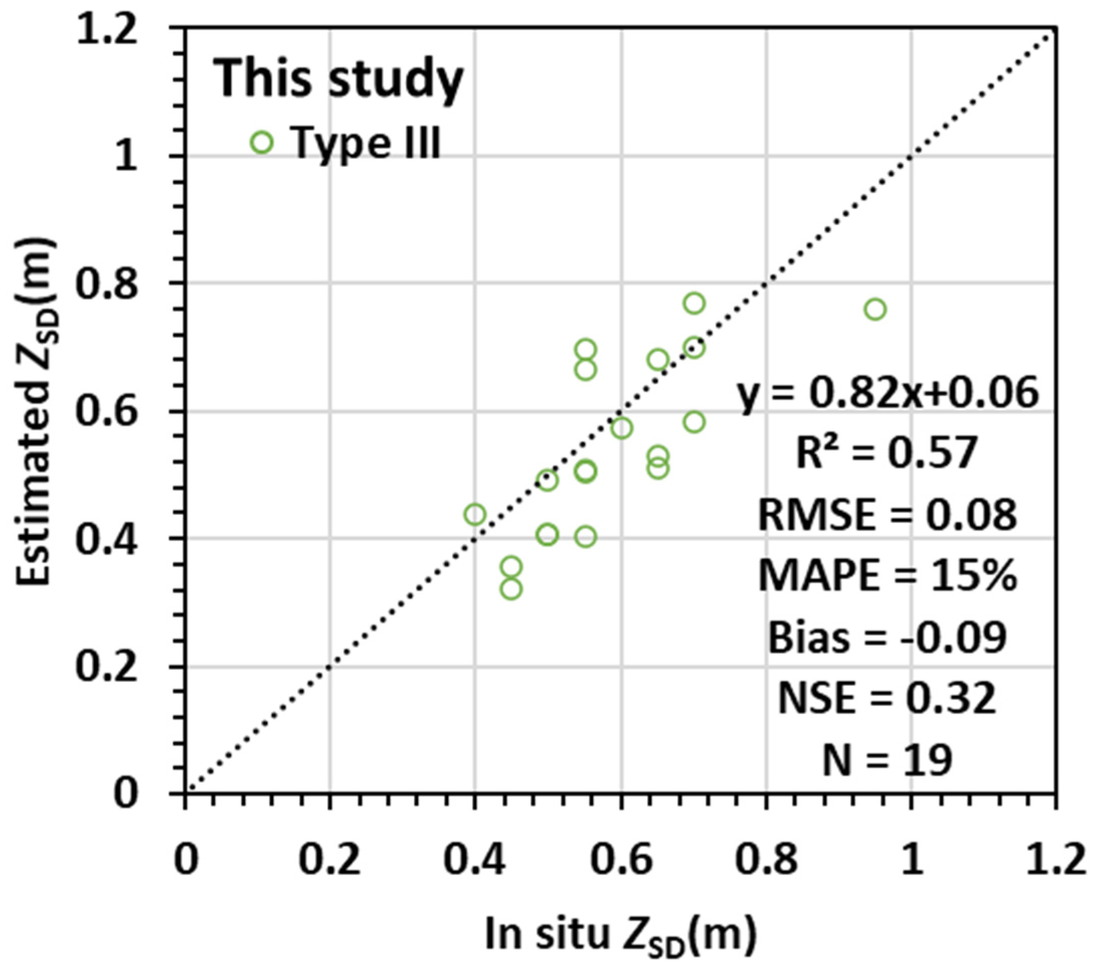
3.1. Validation Using Synthetic Datasets I and III

Figure 4 compares known $Z_{SD}$ values (i.e., Synthetic Dataset III) and estimated $Z_{SD}$ values from Synthetic Dataset I using the Jiang19 algorithm and the algorithm developed in our study, respectively. From the figure, we observed many overestimations around the boundary between Type I and Type II waters as well as around the boundary between Type II and Type III waters when the Jiang19 algorithm was used (Figure 4a). These outliers resulted in very low values of R² (=0.008) and NSE (=−200.12), and high values of RMSE (0.30 in $lo{g}_{10}$ $Z_{SD}$ units), MAPE (116%), and bias (83%). In contrast, the outliers are well addressed in the new algorithm, with improved values of R² (0.97), NSE (0.90), RMSE (0.23 in $lo{g}_{10}$ $Z_{SD}$ units), and MAPE (65%) (Figure 4b). Even when the outliers in Jiang et al.’s results were removed (N = 84,166), our proposed algorithm still performed better than the Jiang19 algorithm, with reduced values of RMSE (0.29 to 0.23 in $lo{g}_{10}$ $Z_{SD}$ units) and MAPE (90% to 68%) as well as increased values of R² (0.95 to 0.97) and NSE (0.85 to 0.90). However, a systematic overestimation was found in the new algorithm (bias of 60%). The results shown in Figure 4a,b are also represented according to the QAA used (Figure 4c,d) and to the selected wavelength with the minimum K_d(λ) (Figure 4e,f). These figures were used to discuss how the proposed estimation algorithm worked (see Section 4).

3.2. Validation Using In Situ Dataset

Figure 5 compares the in situ measured and estimated $Z_{SD}$ values. The estimated $Z_{SD}$ values were obtained from in situ measured $R_{rs}$(λ) spectra using the Jiang19 algorithm or the algorithm developed in this study. The results show that the new $Z_{SD}$ estimation algorithm outperformed the Jiang19 algorithm with a reduced RMSE (from 0.18 to 0.17 in $lo{g}_{10}$ unit) and MAPE (from 32% to 27%) as well as increased NSE (from 0.90 to 0.92) and R² values (from 0.90 to 0.93). In particular, we observed that three points with large errors due to the use of the Jiang19 algorithm (blue circles with red boxes in Figure 5a) were improved substantially by using the new algorithm (Figure 5b). However, compared to the use of the Jiang19 algorithm, the bias due to the use of the new algorithm increased slightly, from a 13% underestimation to an 18% underestimation. In addition, unlike the results shown in Figure 4, systematic overestimation was not found in the application of in situ measured $R_{rs}$(λ) spectra to estimate $Z_{SD}$, regardless of the use of the Jiang 19 algorithm or the new algorithm. Type IV waters were not found from our in situ dataset. As in Figure 4, the results shown in Figure 5a,b are also represented according to the QAA used (Figure 5c,d) and to the selected wavelength with the minimum K_d(λ) (Figure 5e,f). These figures were also used to discuss how the proposed $Z_{SD}$ estimation algorithm worked (see Section 4).

3.3. Validation Using MERIS Data

We further compared the estimated $Z_{SD}$ values from MERIS images using the newly developed algorithm to the in situ measured $Z_{SD}$ values (Figure 6). The in situ measured $Z_{SD}$ values were obtained from the Kasumigaura database, and all matchups were classified to Type III waters based on their MERIS-derived $R_{rs}$(λ) spectra. From the figure, the MERIS-derived $Z_{SD}$ values were consistent with the in situ measured $Z_{SD}$ values, with a MAPE value of 15%, an RMSE value of 0.08 (in $lo{g}_{10}$unit), and a bias value of −9%. The R² value of 0.57 and the slope of 0.82 also indicate the good performance of the new $Z_{SD}$ estimation algorithm. Since the Jiang19 algorithm also selected the same reference band (band 12 of MERIS) and the corresponding QAA (QAA_T754) for all matchups, identical results were obtained when we used the Jiang19 algorithm (data not shown). Systematic overestimation was not found in the application of MERIS data.

4. Discussion

We developed a new algorithm to estimate $Z_{SD}$ from MERIS data. Since this algorithm is based on several existing semianalytical algorithms [21,29,30,31,42], it can be applied to different optical water types, from clear to extremely turbid. The validation results from the synthetic dataset (with a wide range of inherent optical properties, $Z_{SD}$ values ranging from 0.01 to 44.68 m) and the in situ dataset (from 21 Japanese waters, $Z_{SD}$ values ranging from 0.3 to 16.4 m) provide strong evidence to confirm the applicability of the developed $Z_{SD}$ estimation algorithm.

However, a systematic overestimation of $Z_{SD}$ values was observed from the validation results of the use of the synthetic dataset (Figure 4b). This is because the assumption for a$\left(\lambda \right)$ at the reference wavelengths resulted in an underestimation of a$\left(\lambda \right)$ values and thus an underestimation of b_b(λ) values at the same wavelength. These underestimations propagated to the final estimated $Z_{SD}$ values. However, no overestimation of $Z_{SD}$ values was observed when the developed algorithm was applied to the in situ and satellite data (Figure 5b and Figure 6). This is probably because the measurement errors contained in the in situ and satellite data hid (or offset) the systematic overestimation due to the mechanism of the developed algorithm. Therefore, further correction to mitigate the systematic overestimation was not carried out in this study.

Optical water type classification is very important because it helps to both clarify relationships between different properties inside a certain class and quantify the variation between classes [25,47]. Recently, interest has grown in the application of the optical water type classification in the remote sensing of ocean color (e.g., [21,31,48,49,50,51]). In this study, we found that water type classification is a guide to select the most appropriate reference wavelength and corresponding QAA for the more accurate estimation of a$\left(\lambda \right)$ and b_b(λ) in waters with different optical properties. Therefore, we adopted the latest classification algorithm to classify all waters into four types. In contrast, the Jiang19 algorithm classified waters into only two types (clear and turbid) and used two corresponding QAAs (QAA_V5 and QAA_T754), thus generating large errors around boundaries of different water types (Figure 4a). For example, in Figure 4c, the Jiang19 algorithm classified some data samples as the clear water type and used QAA_V5 to estimate a$\left(\lambda \right)$ and b_b(λ); thus, large errors occurred in the $Z_{SD}$ estimations (yellow points in Figure 4c). In contrast, we classified these data samples as Water Type II (moderately turbid waters), which enabled us to use QAA_TM for a$\left(\lambda \right)$ and b_b(λ) estimations and in turn improved the $Z_{SD}$ estimations (blue points in Figure 4d). Similar results can also be observed from Figure 5c. For example, the Jiang19 algorithm classified the yellow point with red box 3 as clear water and two green points with red boxes 1 and 2 as turbid water, and thus used QAA_V5 and QAA_T754 to estimate a$\left(\lambda \right)$ and b_b(λ), resulting finally in large errors in the $Z_{SD}$ estimations. These three $Z_{SD}$ estimations were improved by classifying them as Type II waters and thus using QAA_TM to replace QAA_V5 and QAA_T754 (Figure 5d).

In addition, Jiang et al. [31] suggested the use of QAA_V6 to estimate a$\left(\lambda \right)$ and b_b(λ) at the reference wavelength of 665 nm for Type II waters. However, several previous studies have reported that QAA_V6 often failed in turbid waters [6,21,30,42]. Therefore, we used QAA_TM instead of QAA_V6 in this study. Our results also show that QAA_TM performed better than QAA_V6 for Type II waters (data not shown).

We improved the accuracy of a$\left(\lambda \right)$ and b_b(λ) estimation by classifying waters into four types (effort 1), and then adopted different QAA to estimate a$\left(\lambda \right)$ and b_b(λ) for each water type (efforts 2 and 3). These three efforts addressed most of the outliers caused by using the Jiang19 algorithm. However, some outliers remained after the above three efforts. This is because 620 or 665 nm was sometimes identified as the wavelength with the minimum K_d even for some Type I and II waters due to uncertainty in the Y estimation model [30]. The identification of 620 or 665 nm is obviously inappropriate as the wavelength with the minimum K_d in Type I and II waters should be at 490 or 560 nm based on the statistical results in Figure 3. Therefore, in this study, we also limited the wavelengths used to estimate the minimum$K_d\left(\lambda \right)$ in each water type. This effort can make the wavelengths for estimating minimum $K_d\left(\lambda \right)$ close to the reference wavelength in each water type and thus can reduce errors due to uncertainty in the Y estimation model as seen in Figure 4e,f (not clearly observed in Figure 5e,f).

5. Conclusions

In this study, we developed a semianalytical algorithm for estimating $Z_{SD}$ values from remote sensing data. The developed $Z_{SD}$ estimation algorithm considers different optical properties in four water types, thus allowing the selection of the most optimal reference wavelength and QAA for more accurate estimation of total absorption and backscattering coefficients and, in turn, improved $Z_{SD}$ estimations compared to the previous study. In addition, constraining the wavelength range of minimum$K_d\left(\lambda \right)$ in each water type contributed to the improvement of $Z_{SD}$estimation accuracy. The validation results using synthetic and in situ data show that the developed algorithm is applicable to different optical water types.

References

1. Swift, T.J.; Perez-Losada, J.; Schladow, S.G.; Reuter, J.E.; Jassby, A.D.; Goldman, C.R. Water clarity modeling in Lake Tahoe: Linking suspended matter characteristics to Secchi depth. Aquat. Sci. 2006, 68, 1–15. [Google Scholar] [CrossRef]
2. Doron, M.; Babin, M.; Mangin, A.; Hembise, O. Estimation of light penetration, and horizontal and vertical visibility in oceanic and coastal waters from surface reflectance. J. Geophys. Res. Earth Surf. 2007, 112, C06003. [Google Scholar] [CrossRef] [Green Version]
3. Fleming-Lehtinen, V.; Laamanen, M. Long-term changes in Secchi depth and the role of phytoplankton in explaining light attenuation in the Baltic Sea. Estuar. Coast. Shelf Sci. 2012, 102–103, 1–10. [Google Scholar] [CrossRef]
4. Lee, Z.; Shang, S.; Hu, C.; Du, K.; Weidemann, A.; Hou, W.; Lin, J.; Lin, G. Secchi disk depth: A new theory and mechanistic model for underwater visibility. Remote Sens. Environ. 2015, 169, 139–149. [Google Scholar] [CrossRef] [Green Version]
5. Fukushima, T.; Matsushita, B.; Oyama, Y.; Yoshimura, K.; Yang, W.; Terrel, M.; Kawamura, S.; Takegahara, A. Semi-analytical prediction of Secchi depth using remote-sensing reflectance for lakes with a wide range of turbidity. Hydrobiologia 2015, 780, 5–20. [Google Scholar] [CrossRef]
6. Rodrigues, T.; Alcântara, E.; Watanabe, F.; Imai, N. Retrieval of Secchi disk depth from a reservoir using a semi-analytical scheme. Remote Sens. Environ. 2017, 198, 213–228. [Google Scholar] [CrossRef] [Green Version]
7. Liu, Y.; Xiao, C.; Li, J.; Zhang, F.; Wang, S. Secchi Disk Depth Estimation from China’s New Generation of GF-5 Hyperspectral Observations Using a Semi-Analytical Scheme. Remote Sens. 2020, 12, 1849. [Google Scholar] [CrossRef]
8. Olmanson, L.G.; Bauer, M.E.; Brezonik, P.L. A 20-year Landsat water clarity census of Minnesota’s 10,000 lakes. Remote Sens. Environ. 2008, 112, 4086–4097. [Google Scholar] [CrossRef]
9. Wondie, A.; Mengistu, S.; Vijverberg, J.; Dejen, E. Seasonal variation in primary production of a large high altitude tropical lake (Lake Tana, Ethiopia): Effects of nutrient availability and water transparency. Aquat. Ecol. 2007, 41, 195–207. [Google Scholar] [CrossRef]
10. Canfield, D.E.; Langeland, K.A.; Linda, S.B.; Haller, W.T. Relations between water transparency and maximum depth of macrophyte colonization in lakes. J. Aquat. Plant Manag. 1985, 23, 25–28. [Google Scholar]
11. Lee, Z.; Carder, K.L.; Mobley, C.D.; Steward, R.G.; Patch, J.S. Hyperspectral remote sensing for shallow waters: 2 Deriving bottom depths and water properties by optimization. Appl. Opt. 1999, 38, 3831–3843. [Google Scholar] [CrossRef] [PubMed] [Green Version]
12. Holland, R.E. Changes in Planktonic Diatoms and Water Transparency in Hatchery Bay, Bass Island Area, Western Lake Erie Since the Establishment of the Zebra Mussel. J. Great Lakes Res. 1993, 19, 617–624. [Google Scholar] [CrossRef]
13. Devlin, M.; Barry, J.; Mills, D.; Gowen, R.; Foden, J.; Sivyer, D.; Tett, P. Relationships between suspended particulate material, light attenuation and Secchi depth in UK marine waters. Estuar. Coast. Shelf Sci. 2008, 79, 429–439. [Google Scholar] [CrossRef]
14. McCullough, I.M.; Loftin, C.S.; Sader, S.A. High-frequency remote monitoring of large lakes with MODIS 500 m imagery. Remote Sens. Environ. 2012, 124, 234–241. [Google Scholar] [CrossRef]
15. Bai, S.; Gao, J.; Sun, D.; Tian, M. Monitoring Water Transparency in Shallow and Eutrophic Lake Waters Based on GOCI Observations. Remote Sens. 2020, 12, 163. [Google Scholar] [CrossRef] [Green Version]
16. Sòria-Perpinyà, X.; Pereira-Sandoval, M.; Ruiz-Verdú, A.; Soria, J.M.; Delegido, J.; Vicente, E.; Moreno, J.; Urrego, E.P. Monitoring water transparency of a hypertrophic lake (the Albufera of València) using multitemporal Sentinel-2 satellite images. Limnetica 2020, 39, 373–386. [Google Scholar] [CrossRef]
17. Chang, N.; Luo, L.; Wang, X.C.; Song, J.; Han, J.; Ao, D. A novel index for assessing the water quality of urban landscape lakes based on water transparency. Sci. Total Environ. 2020, 735, 139351. [Google Scholar] [CrossRef]
18. Doron, M.; Babin, M.; Hembise, O.; Mangin, A.; Garnesson, P. Ocean transparency from space: Validation of algorithms estimating Secchi depth using MERIS, MODIS and SeaWiFS data. Remote Sens. Environ. 2011, 115, 2986–3001. [Google Scholar] [CrossRef]
19. Mao, Y.; Wang, S.; Qiu, Z.; Sun, D.; Bilal, M. Variations of transparency derived from GOCI in the Bohai Sea and the Yellow Sea. Opt. Express 2018, 26, 12191–12209. [Google Scholar] [CrossRef]
20. Wang, S.; Lee, Z.; Shang, S.; Li, J.; Zhang, B.; Lin, G. Deriving inherent optical properties from classical water color measurements: Forel-Ule index and Secchi disk depth. Opt. Express 2019, 27, 7642–7655. [Google Scholar] [CrossRef]
21. Jiang, D.; Matsushita, B.; Setiawan, F.; Vundo, A. An improved algorithm for estimating the Secchi disk depth from remote sensing data based on the new underwater visibility theory. ISPRS J. Photogramm. Remote Sens. 2019, 152, 13–23. [Google Scholar] [CrossRef]
22. Vundo, A.; Matsushita, B.; Jiang, D.; Gondwe, M.; Hamzah, R.; Setiawan, F.; Fukushima, T. An Overall Evaluation of Water Transparency in Lake Malawi from MERIS Data. Remote Sens. 2019, 11, 279. [Google Scholar] [CrossRef] [Green Version]
23. Duntley, S.Q. The Visibility of Submerged Objects; Visibility Laboratory, Massachusetts Institute of Technology; Scripps Institution of Oceanography: San Diego, CA, USA, 1952; Volume 74. [Google Scholar]
24. Bowers, D.G.; Roberts, E.M.; Hoguane, A.M.; Fall, K.A.; Massey, G.M.; Friedrichs, C.T. Secchi Disk Measurements in Turbid Water. J. Geophys. Res. Oceans 2020, 125, 1–9. [Google Scholar] [CrossRef] [Green Version]
25. Uudeberg, K.; Ansko, I.; Põru, G.; Ansper, A.; Reinart, A. Using Optical Water Types to Monitor Changes in Optically Complex Inland and Coastal Waters. Remote Sens. 2019, 11, 2297. [Google Scholar] [CrossRef] [Green Version]
26. Liu, X.; Lee, Z.; Zhang, Y.; Lin, J.; Shi, K.; Zhou, Y.; Qin, B.; Sun, Z. Remote Sensing of Secchi Depth in Highly Turbid Lake Waters and Its Application with MERIS Data. Remote Sens. 2019, 11, 2226. [Google Scholar] [CrossRef] [Green Version]
27. Liu, D.; Duan, H.; Loiselle, S.; Hu, C.; Zhang, G.; Li, J.; Yang, H.; Thompson, J.R.; Cao, Z.; Shen, M.; et al. Observations of water transparency in China’s lakes from space. Int. J. Appl. Earth Obs. Geoinf. 2020, 92, 102187. [Google Scholar] [CrossRef]
28. Zeng, S.; Lei, S.; Li, Y.; Lyu, H.; Xu, J.; Dong, X.; Wang, R.; Yang, Z.; Li, J. Retrieval of Secchi Disk Depth in Turbid Lakes from GOCI Based on a New Semi-Analytical Algorithm. Remote Sens. 2020, 12, 1516. [Google Scholar] [CrossRef]
29. Lee, Z.; Carder, K.L.; Arnone, R.A. Deriving inherent optical properties from water color: A multiband quasi-analytical algorithm for optically deep waters. Appl. Opt. 2002, 41, 5755–5772. [Google Scholar] [CrossRef]
30. Yang, W.; Matsushita, B.; Chen, J.; Yoshimura, K.; Fukushima, T. Retrieval of Inherent Optical Properties for Turbid Inland Waters from Remote-Sensing Reflectance. IEEE Trans. Geosci. Remote Sens. 2013, 51, 3761–3773. [Google Scholar] [CrossRef]
31. Jiang, D.; Matsushita, B.; Pahlevan, N.; Gurlin, D.; Lehmann, M.K.; Fichot, C.G.; Schalles, J.; Loisel, H.; Binding, C.; Zhang, Y.; et al. Remotely estimating total suspended solids concentration in clear to extremely turbid waters using a novel semi-analytical method. Remote Sens. Environ. 2021, 258, 112386. [Google Scholar] [CrossRef]
32. Mobley, C.D. Estimation of the remote-sensing reflectance from above-surface measurements. Appl. Opt. 1999, 38, 7442–7455. [Google Scholar] [CrossRef] [PubMed]
33. Jiang, D.; Matsushita, B.; Yang, W. A simple and effective method for removing residual reflected skylight in above-water remote sensing reflectance measurements. ISPRS J. Photogramm. Remote Sens. 2020, 165, 16–27. [Google Scholar] [CrossRef]
34. NIES. Lake Kasumigaura Database, National Institute for Environmental Studies, Japan. 2020. Available online: http://db.cger.nies.go.jp/gem/moni-e/inter/GEMS/database/kasumi/index.html. (accessed on 24 August 2020).
35. Gordon, H.R.; Brown, O.B.; Evans, R.H.; Brown, J.W.; Smith, R.C.; Baker, K.S.; Clark, D.K. A Semianalytic Radiance Model of Ocean Color. J. Geophys. Res. 1988, 93, 10909–10924. [Google Scholar] [CrossRef]
36. Lee, Z.-P.; Du, K.; Arnone, R. A model for the diffuse attenuation coefficient of downwelling irradiance. J. Geophys. Res. Earth Surf. 2005, 110, 1–10. [Google Scholar] [CrossRef]
37. Lee, Z.; Hu, C.; Shang, S.; Du, K.; Lewis, M.; Arnone, R.; Brewin, R. Penetration of UV-visible solar radiation in the global oceans: Insights from ocean color remote sensing. J. Geophys. Res. Oceans 2013, 118, 4241–4255. [Google Scholar] [CrossRef] [Green Version]
38. Zhang, X.; Hu, L. Scattering by pure seawater at high salinity. Opt. Express 2009, 17, 12685–12691. [Google Scholar] [CrossRef]
39. Lee, Z.; Carder, K.L.; Mobley, C.D.; Steward, R.G.; Patch, J.S. Hyperspectral remote sensing for shallow waters. I. A semianalytical model. Appl. Opt. 1998, 37, 6329–6338. [Google Scholar] [CrossRef]
40. Gower, J.; King, S.; Borstad, G.; Brown, L. Detection of intense plankton blooms using the 709 nm band of the MERIS imaging spectrometer. Int. J. Remote Sens. 2005, 26, 2005–2012. [Google Scholar] [CrossRef]
41. Yang, W.; Matsushita, B.; Chen, J.; Yoshimura, K.; Fukushima, T. Application of a Semianalytical Algorithm to Remotely Estimate Diffuse Attenuation Coefficient in Turbid Inland Waters. IEEE Geosci. Remote Sens. Lett. 2014, 11, 1046–1050. [Google Scholar] [CrossRef]
42. Curtarelli, V.P.; Barbosa, C.C.F.; Maciel, D.A.; Júnior, R.F.; Carlos, F.M.; Novo, E.D.M.; Curtarelli, M.; Silva, E. Diffuse Attenuation of Clear Water Tropical Reservoir: A Remote Sensing Semi-Analytical Approach. Remote Sens. 2020, 12, 2828. [Google Scholar] [CrossRef]
43. Joshi, I.D.; D’Sa, E.J. An estuarine-tuned quasi-analytical algorithm (QAA-V): Assessment and application to satellite estimates of SPM in Galveston Bay following Hurricane Harvey. Biogeosciences 2018, 15, 4065–4086. [Google Scholar] [CrossRef] [Green Version]
44. Andrade, C.; Alcântara, E.; Bernardo, N.; Kampel, M. An assessment of semi-analytical models based on the absorption coefficient in retrieving the chlorophyll-a concentration from a reservoir. Adv. Space Res. 2019, 63, 2175–2188. [Google Scholar] [CrossRef]
45. Deng, L.; Zhou, W.; Cao, W.; Wang, G.; Zheng, W.; Xu, Z.; Li, C.; Yang, Y.; Xu, W.; Zeng, K.; et al. Evaluating semi-analytical algorithms for estimating inherent optical properties in the South China Sea. Opt. Express 2020, 28, 13155–13176. [Google Scholar] [CrossRef] [PubMed]
46. Lee, Z.; Carder, K.L.; Arnone, R. Update of the Quasi-Analytical Algorithm (QAA_v6); International Ocean Colour Coordnating Group—IOCCG: Monterey, CA, USA, 2014. [Google Scholar]
47. Reinart, A.; Herlevi, A.; Arst, H.; Sipelgas, L. Preliminary optical classification of lakes and coastal waters in Estonia and south Finland. J. Sea Res. 2003, 49, 357–366. [Google Scholar] [CrossRef]
48. Moore, T.S.; Dowell, M.D.; Bradt, S.; Verdu, A.R. An optical water type framework for selecting and blending retrievals from bio-optical algorithms in lakes and coastal waters. Remote Sens. Environ. 2014, 143, 97–111. [Google Scholar] [CrossRef] [PubMed] [Green Version]
49. Matsushita, B.; Yang, W.; Yu, G.; Oyama, Y.; Yoshimura, K.; Fukushima, T. A hybrid algorithm for estimating the chlorophyll-a concentration across different trophic states in Asian inland waters. ISPRS J. Photogramm. Remote Sens. 2015, 102, 28–37. [Google Scholar] [CrossRef] [Green Version]
50. Spyrakos, E.; O’Donnell, R.; Hunter, P.D.; Miller, C.; Scott, M.; Simis, S.G.H.; Neil, C.; Barbosa, C.C.F.; Binding, C.E.; Bradt, S.; et al. Optical types of inland and coastal waters. Limnol. Oceanogr. 2018, 63, 846–870. [Google Scholar] [CrossRef] [Green Version]
51. Balasubramanian, S.V.; Pahlevan, N.; Smith, B.; Binding, C.; Schalles, J.; Loisel, H.; Gurlin, D.; Greb, S.; Alikas, K.; Randla, M.; et al. Robust algorithm for estimating total suspended solids (TSS) in inland and nearshore coastal waters. Remote Sens. Environ. 2020, 246, 111768. [Google Scholar] [CrossRef]
Figure 1. Study areas: (a) Locations of 20 Japanese lakes and Tokyo Bay and (b) sampling sites of the Lake Kasumigaura database.
Remotesensing 14 00868 g001
Figure 2. Flowchart of the Z S D estimation algorithm proposed in this study.
Remotesensing 14 00868 g002
Figure 3. Statistical analysis using Synthetic Dataset II to identify the possibility of a minimum K d ( λ ) for each water type.
Remotesensing 14 00868 g003
Figure 4. Comparison of known and estimated Z S D values. The estimated Z S D values were obtained from the simulated R r s ( λ ) in Synthetic Dataset I using the Jiang19 algorithm (a,c,e) and the new algorithm proposed in this study (b,d,f). The colors in the figures represent water types (a,b), the QAA used (c,d), and the wavelengths with the minimum K d ( λ ) (e,f).
Remotesensing 14 00868 g004aRemotesensing 14 00868 g004b
Figure 5. Comparison of in situ measured and estimated Z S D values. The estimated Z S D values were obtained from in situ measured R r s ( λ ) spectra using the Jiang19 algorithm (a,c,e) and the new algorithm proposed in this study (b,d,f). The colors in the figures represent water types (a,b), the QAA used (c,d), and the wavelengths with the minimum K d ( λ ) (e,f).
Remotesensing 14 00868 g005
Figure 6. Comparisons of the in situ measured Z S D values and the estimated Z S D values from MERIS data using the new Z S D estimation algorithm.
Remotesensing 14 00868 g006