Stepwise Fusion of Hyperspectral, Multispectral and Panchromatic Images with Spectral Grouping Strategy: A Comparative Study Using GF5 and GF1 Images

Abstract

Since hyperspectral satellite images (HSIs) usually hold low spatial resolution, improving the spatial resolution of hyperspectral imaging (HSI) is an effective solution to explore its potential for remote sensing applications, such as land cover mapping over urban and coastal areas. The fusion of HSIs with high spatial resolution multispectral images (MSIs) and panchromatic (PAN) images could be a solution. To address the challenging work of fusing HSIs, MSIs and PAN images, a novel easy-to-implement stepwise fusion approach was proposed in this study. The fusion of HSIs and MSIs was decomposed into a set of simple image fusion tasks through spectral grouping strategy. HSI, MSI and PAN images were fused step by step using existing image fusion algorithms. According to different fusion order, two strategies ((HSI+MSI)+PAN and HSI+(MSI+PAN)) were proposed. Using simulated and real Gaofen-5 (GF-5) HSI, MSI and PAN images from the Gaofen-1 (GF-1) PMS sensor as experimental data, we compared the proposed stepwise fusion strategies with the traditional fusion strategy (HSI+PAN), and compared the performances of six fusion algorithms under three fusion strategies. We comprehensively evaluated the fused results through three aspects: spectral fidelity, spatial fidelity and computation efficiency evaluation. The results showed that (1) the spectral fidelity of the fused images obtained by stepwise fusion strategies was better than that of the traditional strategy; (2) the proposed stepwise strategies performed better or comparable spatial fidelity than traditional strategy; (3) the stepwise strategy did not significantly increase the time complexity compared to the traditional strategy; and (4) we also provide suggestions for selecting image fusion algorithms using the proposed strategy. The study provided us with a reference for the selection of fusion strategies and algorithms in different application scenarios, and also provided an easy-to-implement solution and useful references for fusing HSI, MSI and PAN images.

1. Introduction

In recent years, with the launches of various hyperspectral satellites [1], hyperspectral images (HSIs) have been frequently used in many applications, such as coastal wetland mapping, species classification of mangrove forests, and so on. HSIs with detailed spectral information are particularly important in the analysis of the land-cover for coastal environmental monitoring, disaster monitoring, precision agriculture, forestry surveying and urban planning [1], because HSIs with high spectral resolution can provide better performance for qualitative and quantitative analysis of geographic entities. However, limited by the sensitivity of photoelectric sensors and transmission capability, the spatial resolution of HSIs is not sufficient for some applications [2], such as the monitoring of air pollution [3], land and sea surface temperatures [4,5], heavy metals in soil and vegetation [6], water quality [7], land cover [8,9] and lithological mapping [10]. In recent years, the development of accurate remote sensing applications has increased the requirement for images with both high spatial and spectral resolution.

The fusion of HSIs with high spatial resolution images is an excellent solution to obtain images with both high spectral and spatial resolution [11]. Image fusion can break through the mutual restriction of spatial and spectral resolution [12], integrate the advantages of HSIs and high spatial resolution images, and obtain HSIs with high spatial resolution [13,14]. Integrating the complementary advantages of HSI, MSI and PAN images in the same area through image fusion technology will greatly improve the application potential and prospects of all three. According to different combinations of input data source, HSI fusion strategies can be divided into three categories: (1) HSI+MSI, (2) HSI+PAN and (3) HSI+MSI+PAN. Currently, most of the HSI fusion studies have focused on the first two categories, and few studies have focused on the last category.

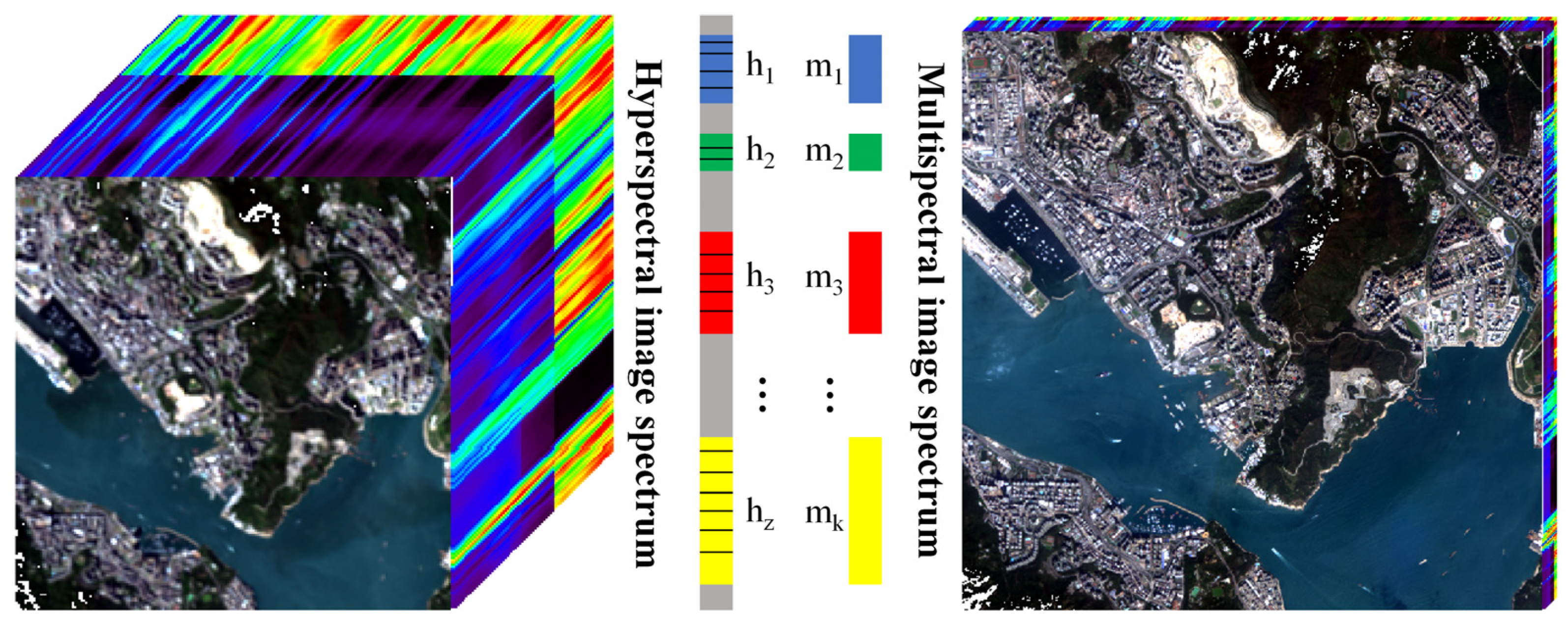
Since pan-sharpening can be considered a special case of the HSI–MSI fusion problem, spectral grouping strategies have been proposed to generalize existing pan-sharpening methods to the more challenging HSI–MSI fusion. Specifically, an HSI–MSI fusion framework was proposed in [15] which divided HSIs into multiple groups of images according to spectrum and fused the groups with their corresponding channels of MSIs. A similar idea was also proposed in [2], in which the HSI–MSI fusion was automatically decomposed into multiple groups of weighted pan-sharping problems. Selva et al. also proposed a framework called hyper-sharpening that effectively applied the MRA-based pan-sharpening methods to HSI–MSI fusion [16]. Fusing images by exploiting the inherent spectral characteristics of the scene via a subspace is another method for HSI–MSI fusing [12,14,17,18], and a Bayesian method based on a maximum a posteriori (MAP) estimation which used a stochastic mixing model (SMM) to estimate the underlying spectral scene was one of the first proposed methods [12]. Another kind of popular approach for fusing HSI and MSI was spectral unmixing, and several methods were proposed [19,20,21]. Unmixing-based fusion obtained endmember information and high-resolution abundance matrices from the HSI and MSI, and the fused image can be reconstructed by multiplying the two resulting matrices.

HSI–MSI fusion can only obtain HSIs with the same spatial resolution as the MSIs. To obtain HSIs with higher spatial resolution, several HSI–PAN fusion methods were proposed [22,23,24,25]. However, most of the existing HSI–PAN fusion methods focused on increasing the spatial resolution by two–five times. In [22,24,25], the spatial resolution ratios of several groups of HSI and PAN image were three times and five times, and in [23], it was three times. In practical applications, the HSI fusion problems with spatial resolution ratios of 10 times or more are challenging [26].

Considering the limitations of HSI–MSI and HSI–PAN fusion, HSI–MSI–PAN fusion is a potential solution. Using the integrated fusion framework proposed by Meng et al., spatial (high-frequency) and spectral (low-frequency) components of multi-sensor images were decomposed using modulation transfer function (MTF) filtering, and then they were fused by automatically estimating the fusion weights [27]. Shen et al. also proposed an integrated method for fusing multiple temporal-spatial-spectral scales of remote sensing images. The method was designed based on the maximum a posteriori (MAP) framework [28], and the efficacy of the method was only validated using simulated images. Besides, the fusion of HSI–MSI–PAN is theoretically complex, and there are few reliable methods validated with real data available at present. How to fuse HSI–MSI–PAN simply and effectively is still an urgent problem to be solved.

To the best of our knowledge, in terms of the strategy for fusing HSI, MSI and PAN images, existing studies in the literature have generally adopted the integrated fusion strategy [27,28], and have not explicitly proposed the concept of stepwise fusion. Since the spectral grouping strategy has been successfully applied in the literature [2,15,16] and many MSI–PAN fusion algorithms have been proposed, can HSI–MSI–PAN fusion be theoretically simplified into several groups of sequential HSI–PAN fusion problems?

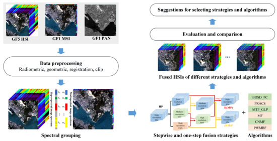
Therefore, the aim of this study is to explore the effectiveness of fusing HSI, MSI and PAN images using stepwise and spectral grouping strategies with existing pan-sharping algorithms, and also to compare the performances of different algorithms. With HSIs of Gaofen-5 (GF-5), MSIs and PAN images obtained from the Gaofen-1 (GF-1) PMS sensor as a case, an easy-to-implement stepwise and spectral grouping approach for fusing HSI, MSI and PAN images was proposed and evaluated. Adopting the stepwise and spectral grouping strategy, the fusion of HSI, MSI and PAN images was decomposed into a set of MSI–PAN fusion problems, and six state-of-the-art pan-sharpening algorithms were evaluated and compared within this framework.

The rest of this paper was organized as follows: In Section 2, the study area and image data are introduced. The stepwise and spectral grouping approach, as well a comparison of MSI–PAN fusion algorithms are described in Section 3. In Section 4, we compare the performances of different fusion strategies and algorithms, considering different image types. Some important issues are discussed in Section 5, and the final conclusions are drawn in Section 6.

2. Materials

2.1. Study Area and Image Data

A group of GF-5 HSI, GF-1 MSI and PAN images partially covering Hong Kong, China, were used in this study. Hong Kong (22°08′ N–22°35′ N, 113°49′ E–114°31′ E) is a coastal city located in the south of China. As shown in Figure 1, the image contains multiple types of geographical entities such as buildings, roads, vegetation, water, etc. The difference between the capturing times (acquisition time of images in

Table 1. Details of GF5 and GF1 optical sensors.

Image Data	GF-5 HSI	GF-1 MSI	GF-1 PAN
Launch time of sensors	9 May 2018	26 April 2013	26 April 2013
Spectral range/nm	400–2500	450–520	450–900
		520–590
		630–690
		770–890
Number of bands	330	4	1
Spectral resolution/nm	5 (VNIR)	-	-
	10 (SWIR)	-	-
Spatial resolution/m	30	8	2
Acquisition time of images	5 October 2018	2 October 2018	2 October 2018

) of the three images is only 3 days, which may avoid feature differences in time scale.

The GF-5 satellite was successfully launched on 9 May 2018 [29]. The visible shortwave infrared hyperspectral camera of the GF-5 satellite can obtain 330 spectral channel data in the spectral range from visible light to shortwave infrared (400–2500 nm) at a spatial resolution of 30 m. The spectral resolution of the VNIR and SWIR spectrometer is 5 nm and 10 nm [1], respectively. The GF-1 satellite was successfully launched on 26 April 2013 [30]. The GF-1 satellite is equipped with two panchromatic/multispectral (PMS) cameras and four wide field view cameras. The PMS data have four spectral bands at 8 m spatial resolution and a panchromatic (PAN) band at 2 m spatial resolution with the spectrum ranging from 450 to 900 nm [31]. The details of GF-5 and GF-1 optical sensors are shown in Table 1.

2.2. Data Preprocessing

Data preprocessing work was carried out first, including radiometric calibration, atmospheric correction, ortho correction, image registration, and image clipping. First of all, the GF-5 HSI, GF-1 MSI and PAN image were calibrated according to the absolute radiance calibration coefficients of satellites. The digital number (DN) of GF-5 HSI and GF-1 MSI was calibrated to the radiance; the DN of GF-1 PAN image was calibrated to the top of atmosphere reflectance. Fast line-of-sight atmosphere (FLAASH) atmospheric correction was performed on the GF-5 HSI and GF-1 MSI to obtain the surface reflectance. ASTER GDEM 30 m resolution digital elevation data (http://www.gscloud.cn, accessed on 30 December 2021) was used to orthorectify the three images, and the images were resampled using the cubic convolution method. GF-5 HSI and GF-1 PAN were registered with high accuracy based on GF-1 MSI. To facilitate the subsequent fusion experiments, GF-5 HSI was sampled from 30 m to 32 m. On the premise that the three images have been registered with high precision, the aligned data covering the same area can be easily obtained by clipping the three images with the same vector range. Slight alignment deviations due to excessively large resolution ratios (such as 32 m and 2 m) were unavoidable, however their impact on fusion was minimal and was ignored in our study.

3. Methods

3.1. Grouping Fusion Framework

Hyperspectral remote sensing images with hundreds of nanometer-wide narrow bands can obtain continuous and fine spectral responses of targets within a certain spectral range [32]. The spectrum of multispectral image has local discontinuities, and the spectral ranges of HSI and MSI do not completely overlap. The fusion of HSI and MSI in the non-overlapping spectral range usually causes spectral distortion [33].Therefore, some studies proposed the HSI–MSI grouping fusion framework [2,15,16], which can retain the local spectral information of images and minimize spectral distortion by fusing the images of each overlapping spectral interval one by one [15].

For HSIs and MSIs from the same scene, it is assumed that the HSI has P bands, the MSI has Q bands, and P > Q. As shown in Figure 2, the Q bands of MSI are divided into x spectral intervals m_x (x = 1, 2, 3,…, Q) band by band. According to the spectral correspondences between HSI and MSI, the P bands of HSI are divided into y spectral intervals h_y (y = 1, 2, 3,…, Q), and each spectral interval is a multi-band image. The spectral intervals where HSI and MSI do not overlap (the gray region in Figure 2) do not participate in the image fusion process.

The spectra of GF-5 HSI and GF-1 MSI can be divided into four overlapping spectral intervals: 450–520 nm, 520–590 nm, 630–690 nm and 770–890 nm. The corresponding bands of GF-5 HSI and GF-1 MSI in each spectral interval are shown in

Table 2. Spectrums of GF-5 HSI and GF-1 MSI.

Group	Spectral Interval (nm)	GF-1 MSI Band Index	GF-5 HSI Band Index
1	450–520	1	15–31
2	520–590	2	32–47
3	630–690	3	57–71
4	770–890	4	90–118

.

According to the spectral correspondences in Figure 2 and Table 2, the spectral overlaps of HSI and MSI are first obtained. As shown in Figure 3, the single MSI band (MSI₁, MSI₂,…, MSI_n) and multiple HSI groups (HSI₁, HSI₂,…, HSI_n) are then fused in groups to obtain multiple sets of fused images (HSI_MSI₁, HSI_MSI₂,…, HSI_MSI_n). Finally, multiple sets of fused images are stacked by wavelength to get the final fused image (HSI_MSI). This grouping fusion framework simplifies the HSI–MSI fusion into several groups of image fusion tasks, in which a multi-band image is fused with a single-band image. In such cases, a single task can be easily implemented using traditional fusion methods, such as the six fusion algorithms mentioned in this study.

3.2. Stepwise Fusion Approach

Grouping fusion strategy is an effective solution for HSI–MSI fusion. However, to obtain HSIs with higher spatial resolution, higher spatial resolution panchromatic images should be used. Two stepwise approaches could be adopted to fuse HSI, MSI and PAN images, and HSI and PAN images can also be fused directly (Figure 4).

(1) Strategy (HM)P (HSI+MSI)+PAN: A Low spatial resolution HSI and a medium spatial resolution MSI are first fused using the above-mentioned grouping fusion framework. A medium spatial resolution HSI is obtained and then further fused with high spatial resolution PAN image to obtain a high spatial resolution HSI.

(2) Strategy H(MP) HSI+(MSI+PAN): A medium spatial resolution MSI and a high spatial resolution PAN image are first fused. A high spatial resolution MSI is obtained and then further fused with a low spatial resolution HSI using spectral grouping, and a high spatial resolution HSI is obtained.

(3) Strategy HP HSI+PAN: The most common and traditional method is to adopt a directly HSI–PAN fusion, which can be directly implemented by many image fusion algorithms.

The low, medium, and high spatial resolutions are defined relative to the resolution of the HSI, MSI and PAN images, and do not represent the specific spatial resolutions.

3.3. Image Fusion Algorithms

The PAN-sharpening algorithms can be roughly cataloged into three types [34,35,36]: component substitution-based (CS-based), multi-resolution analysis-based (MRA-based), and subspace-based methods. The CS-based, MRA-based and subspace-based approaches have been also extended from multispectral (MS) PAN-sharpening to hyperspectral pan-sharpening [22]. Latest representative algorithms of these three categories are band-dependent spatial-detail-based approaches with physical constraints (BDSD_PC) [37], partial replacement adaptive component substitution (PRACS) [38], modulation transfer function-generalized Laplacian pyramid (MTF_GLP) [35,39], morphological filters (MF) [40], coupled nonnegative matrix factorization (CNMF) [21], principal component analysis/wavelet model-based fusion (PWMBF) [41]. The codes of these algorithms are publicly available for academical purpose through http://openremotesensing.net/kb/codes/ (accessed on 30 December 2021).

3.3.1. CS-Based Methods: BDSD_PC and PRACS

The CS-based methods use matrix transformation to project the HSI/MSI into a new feature space, in which the spatial information is separated from the spectral information. After histogram matching, the components containing the spatial information are replaced with the PAN to realize the sharpening of the transformed HSI/MSI. Finally, by inversely transforming the data, the HSI/MSI is restored to the original space, and the sharpening of the HSI/MSI is completed [42]. The algorithms belonging to this class used in this study are BDSD_PC [37] and PRACS [38].

The band-dependent spatial-detail-based (BDSD) approach [43] started from an extended version of the generic CS-based method. When we are looking for a more robust solution, physical constraints (PS) are widely used. Thus, a physically constrained optimization called BDSD_PC which can improve the quality of the fused images, has been proposed recently. The BDSD_PC algorithm is detailed in [37].

A new adaptive fusion method based on component substitution has been proposed to merge PAN with HSI/MSI. This method generates high-/low-resolution synthetic component images by partial replacement and uses statistical ratio-based high-frequency injection [38]. In other words, the PAN image is not directly used for component substitution. The method is referred to as PRACS, and the specific implementation details of the algorithm are shown in [38].

3.3.2. MRA-Based Methods: MTF_GLP and MF

The MRA-based methods originate from multi-resolution analysis. The method first resamples the HSI/MSI, and then injects the spatial details of the PAN into the resampled HSI/MSI to improve spatial resolution [35]. Two typical MRA-based methods are MTF_GLP [35] and MF [40].

For MTF_GLP, the low-pass filtering is performed for PAN using a gaussian modulation transfer function (MTF) filter. By subtracting filtered PAN from the original PAN, the high spatial detail image is obtained. Then, by using the global gain coefficient, the method injects the extracted detail image into HSI/MSI [35,39].

Restaino, etc. studied the application of nonlinear image decomposition schemes to data fusion [40]. The nonlinear MRA scheme is implemented with a morphological pyramid based on morphological half gradients. The approach can be recast into the general MRA fusion scheme. Due to the use of morphological filters for the detail extraction phase, this method is called MF [44].

3.3.3. Subspace-Based Methods: CNMF and PWMBF

Subspace-based methods include unmixing-based approaches and Bayesian-based approaches [36]. CNMF is a typical unmixing-based approach. The HSI/MSI and PAN are unmixed by alternately using nonnegative matrix factorization (NMF) [45] to obtain the hyperspectral endmember and high-spatial-resolution abundance matrices. Fused images can be obtained by combining these two matrices [21].

By maximizing a posteriori (MAP) probability density of the full-resolution images, Bayesian-based approaches enhance spatial resolution [35,46]. We used one typical Bayesian-based approach named PMWBF. The PWMBF method can handle HSI, MSI and PAN based on the MAP estimation of the undecimated wavelet transform (UDWT) coefficients for the principal components (PCs) of the fused image. The fusion is performed in the lower dimensional PC subspace; therefore, we only need to estimate the first few PCs, instead of every spectral reflectance band. This algorithm is detailed in [41].

3.4. Evaluation of Image Fusion Performances

The performance of an image fusion algorithm was evaluated from three aspects: spectral fidelity, spatial fidelity and computation efficiency measures. The qualitative evaluation used visual interpretation, and the quantitative evaluation used four commonly used quantitative indicators, including spectral angle mapper (SAM) [44], relative dimensionless global error in synthesis (ERGAS) [35], peak signal-to-noise ratio (PSNR) and spatial correlation coefficient (SCC) [35]. The first three indicators evaluated the spectral fidelity, and the last indicator evaluated the spatial fidelity.

3.4.1. Spectral Metrics

SAM [44] calculates the spectral angle between corresponding pixels of reference and fused images. The SAM index at the j-th pixel is defined as:

$$\mathrm{SAM}({\mathbf{v}}_{\mathrm{j}},{\widehat{\mathbf{v}}}_{\mathrm{j}})=\arccos (\frac{{\mathbf{v}}_{\mathrm{j}}^{\mathrm{T}}{\widehat{\mathbf{v}}}_{\mathrm{j}}}{{||{\mathbf{v}}_{\mathrm{j}}||}_2{||{\widehat{\mathbf{v}}}_{\mathrm{j}}||}_2})$$

(1)

where v is the reference image, $\widehat{\mathbf{v}}$ is the fused image and v_j∈R^n×1 and ${\widehat{\mathbf{v}}}_{\mathrm{j}}$∈R^n×1 represent the spectral signatures of the j-th pixel in the reference image and the fused image. A larger SAM means a more severe spectral distortion of the fused images. A SAM value equal to zero denotes absence of spectral distortion [47].

In 2000, Ranchin and Wald proposed ERGAS [48], which provides a global statistical measure of spectral distortion of the quality of the fused data [35], it is defined as:

$$\mathrm{ERGAS}(\mathbf{x},\hat{\mathbf{x}})=100\mathrm{d}\sqrt{\frac{1}{\mathrm{m}}\sum _{\mathrm{i}=1}^{\mathrm{m}}\frac{{||{\mathbf{x}}_{\mathrm{i}}-{\widehat{\mathbf{x}}}_{\mathrm{i}}||}_2^2}{{\left(\frac{1}{\mathrm{n}}{1}_{\mathrm{n}}^{\mathrm{T}}{\mathbf{x}}_{\mathrm{i}}\right)}^2}}$$

(2)

where x_i∈R^n×1 and ${\widehat{\mathbf{x}}}_{\mathrm{i}}$∈R^n×1 represent the i-th band of the reference image and fused image, respectively, d is the ratio of the spatial resolution between the HSI and PAN images and n is the number of pixels in the images. A larger ERGAS means greater spectral distortion.

The PSNR evaluates the spatial reconstruction quality of fused images. It is the ratio between the maximum power of a signal and the power of residual errors [35], which is defined as:

$$\mathrm{PSNR}({\mathbf{x}}_{\mathrm{i}},{\widehat{\mathbf{x}}}_{\mathrm{i}})=10\times {\log }_{10}(\frac{\max {\left({\mathbf{x}}_{\mathrm{i}}\right)}^2}{{||{\mathbf{x}}_{\mathrm{i}}-{\widehat{\mathbf{x}}}_{\mathrm{i}}||}_2^2/\mathrm{P}})$$

(3)

where max(x_i) is the maximum pixel value in the i-th reference band image. A larger PSNR value indicates a better result.

3.4.2. Spatial Metrics

SCC [35] is used to measure the spatial information correlation of two images. Edge detection technology (Sobel operator is used in this study) is used to extract edge information from fused and PAN images. Using the edges from PAN image as reference, the correlation coefficient between the edges from fused and PAN images is calculated. The SCC is defined as follows:

$$\mathrm{SCC}(\mathbf{M},\mathbf{N})=\frac{{\sum }_{\mathrm{i}=1}^{\mathrm{e}}({\mathbf{M}}_{\mathrm{i}}-\stackrel{\_}{\mathbf{M}})({\mathbf{N}}_{\mathrm{i}}-\stackrel{\_}{\mathbf{N}})}{\sqrt{{\sum }_{\mathrm{i}=1}^{\mathrm{e}}{({\mathbf{M}}_{\mathrm{i}}-\stackrel{\_}{\mathbf{M}})}^2{\sum }_{\mathrm{i}=1}^{\mathrm{e}}{({\mathbf{N}}_{\mathrm{i}}-\stackrel{\_}{\mathbf{N}})}^2}}$$

(4)

where M and N are the reference edge image and the edge image to be evaluated. M_i and N_i are samples of M and N; e is the total number of samples; $\stackrel{\_}{\mathbf{M}}$ and $\stackrel{\_}{\mathbf{N}}$ are the mean of M and N. The range of SCC is between 0 and 1, and a high SCC indicates that the similarity of spatial information between the fused image and the reference image is high.

3.4.3. Computational Efficiency Metrics

The running time is recorded to evaluate the computational efficiency of different fusion strategies and algorithms, and the unit of running time is seconds. All the fusion methods were implemented in MATLAB R2020a, and their codes were run on a Win10 computer with an Intel Core i7-9700 processor and 40 GB RAM.

4. Experimental Results

4.1. Experimental Setup

Two groups of HSI, MSI and PAN images were used in this study. Following the above stepwise approaches, 2 m HSI can be obtained by fusing GF-5 HSI, GF-1 MSI and PAN images. However, no 2 m HSI can be used as a reference image to quantitatively evaluate the spectral fidelity of the fused image. Therefore, the spectral fidelities of fusing real GF-5 and GF-1 images were only qualitatively evaluated, while the spatial fidelities were qualitatively and quantitatively evaluated.

The quality of a fused image can be evaluated on the degraded spatial scale [49]. Therefore, simulated images can also be used to evaluate image fusion performances. A group of simulated images were obtained by downsampling the real HSI, MSI and PAN images. The details of simulated images are shown in

Table 3. Details of simulated and real experimental data.

Data	Multi-Source Images	Spatial Resolution(m)	Image Size
Simulated Data	GF-5 HSI	512	50 × 50
	GF-1 MSI	128	200 × 200
	GF-1 PAN	32	800 × 800
Real Data	GF-5 HSI	32	80 × 80
	GF-1 MSI	8	320 × 320
	GF-1 PAN	2	1280 × 1280

. Since real 32 m/pixel GF-5 HSI can used as a reference image, a fused 32 m/pixel HSI was quantitatively and qualitatively evaluated in this study.

For each group of images, comparative experiments were carried using (HM)P, H(MP) and HP strategies, and BDSD_PC, PRACS, MTF_GLP, MF, CNMF and PWMBF algorithms, respectively. The details of these strategies and algorithms are presented in Figure 4 and Section 3.3.

In this section, we first present and compare the results over the full scenes, and then we compare the fusion performances over vegetation and built-up areas. For vegetation areas, the spectral signature is more important for classifying vegetation species and retrieval biochemical indices. However, for built-up areas, the spatial details might be more important to recognize land use types. Therefore, we mainly focus on evaluating the spectral distortion over vegetation areas and evaluating spatial distortion over built-up areas.

4.2. Performance over the Whole Image

4.2.1. Performance Using Simulated Images

The spatial resolution of images obtained by fusing the simulated HSI–MSI–PAN images is 32 m/pixel. The reference and fused images are displayed in true color with the same band combination (R: 639 nm; G: 549 nm; B: 472 nm). Figure 5 shows the fused results of simulated GF5 and GF1 images.

Table 4. SAM index of fusion results using simulated GF5 and GF1 images. A smaller value indicates better performance.

Algorithm	(HM)P	H(MP)	HP	Mean
BDSD_PC	11.112	10.722	8.816	10.217
PRACS	4.787	4.674	5.298	4.920
MTF_GLP	5.242	4.905	5.806	5.318
MF	4.652	3.866	4.964	4.494
CNMF	3.900	4.181	4.353	4.145
PWMBF	4.840	5.424	6.290	5.518

,

Table 5. ERGAS index of fusion results using simulated GF5 and GF1 images. A smaller value indicates better performance.

Algorithm	(HM)P	H(MP)	HP	Mean
BDSD_PC	2.052	2.080	2.272	2.135
PRACS	1.584	1.585	1.873	1.681
MTF_GLP	1.531	1.521	1.830	1.628
MF	1.698	1.574	1.831	1.701
CNMF	1.604	1.627	1.803	1.678
PWMBF	1.534	1.593	1.863	1.663

,

Table 6. PSNR index of fusion results using simulated GF5 and GF1 images. A larger value indicates better performance.

Algorithm	(HM)P	H(MP)	HP	Mean
BDSD_PC	61.335	61.130	60.051	60.838
PRACS	66.731	66.689	63.621	65.680
MTF_GLP	67.417	67.519	63.819	66.252
MF	65.451	67.037	63.785	65.424
CNMF	66.215	65.880	63.964	65.353
PWMBF	67.465	66.738	63.477	65.893

,

Table 7. SCC index of fusion results using simulated GF5 and GF1 images. A larger value indicates better performance.

Algorithm	(HM)P	H(MP)	HP	Mean
BDSD_PC	0.823	0.835	0.583	0.747
PRACS	0.658	0.657	0.520	0.612
MTF_GLP	0.701	0.694	0.576	0.657
MF	0.908	0.886	0.945	0.913
CNMF	0.905	0.914	0.934	0.918
PWMBF	0.830	0.852	0.722	0.801

and

Table 8. Computational time (in seconds) of fusing simulated GF5 and GF1 images. The background color here is to mark the total running time of the strategies (HM)P, H(MP) and HP, respectively, so as to distinguish it from the separate running time of the step 1 and step 2.

Algorithm	(HM)P			H(MP)			HP	Mean
	Step 1	Step 2	Total	Step 1	Step 2	Total
BDSD_PC	14.852	13.856	28.708	0.740	5.246	5.986	12.976	15.890
PRACS	54.654	171.978	226.633	0.839	52.129	52.967	202.296	160.632
MTF_GLP	2.590	25.044	27.633	1.534	8.867	10.400	8.404	15.479
MF	6.207	6.348	12.556	0.455	9.031	9.486	8.264	10.102
CNMF	5.802	33.179	38.981	4.734	48.049	52.783	19.015	36.926
PWMBF	1.021	3.940	4.961	1.652	8.101	9.753	3.929	6.214

present the SAM, ERGAS, PSNR, SCC and computational efficiency of the fused images, respectively. The mean values of the quantitative metrics obtained by the same fusion algorithm with three fusion strategies are shown in the last column of the tables, and the last column (Mean) in the tables below has the same meaning.

Visual evaluation of spectral and spatial distortions: Comparing the results of the three rows in Figure 5, the strategies (HM)P and H(MP) are generally better than the HP strategy in terms of spectral and spatial fidelity. The results of the (HM)P and H(MP) strategies are visually similar. Through our visual comparison, the spatial details of the BDSD_PC, MF and CNMF algorithms are much better than others. The results of these algorithms are similar from the perspective of spectral fidelity, and only the vegetation areas of the results using BDSD_PC algorithm are slightly brighter.

Quantitative evaluation of spectral and spatial distortions: The quantitative evaluation results further confirmed that under most algorithms, strategies (HM)P and H(MP) perform better than HP, with only a few exceptional cases. For example, using HP strategy, the results of MF and CNMF algorithms are slightly better than (HM)P and H(MP) in terms of spatial fidelity. For all algorithms, the performances of (HM)P and H(MP) strategies are equivalent. In terms of spectral fidelity, as can be seen from the last column of Table 4, Table 5 and Table 6, the BDSD_PC algorithm performed the worst, and the performances of the other five algorithms were not much different. It can be seen from the last column of Table 7 that the results using CNMF and MF have the best spatial fidelity, followed by PWMBF and BDSD_PC, MTF_GLP, and the worst is PRACS.

Computational efficiency evaluation: Using four algorithms (MTF_GLP, MF, CNMF and PWMBF), the computational efficiency of strategy HP is better than those of strategies (HM)P and H(MP), but there is not much difference. It is worth noting that the efficiency of H(MP) is much higher than that of (HM)P and HP when using BDSD_PC and PRACS algorithms. As can be seen from Table 8, the fusion of a single-band image and a 77-band image in HP and the second step of (HM)P consumes too much time. However, with the fewer bands involved in each fusion in the H(MP) strategy, the computational time decreased dramatically, which indicated that the time complexity of CS-based algorithms may be related to the number of bands in the image. The efficiency of the H(MP) strategy is generally better than that of (HM)P, except for the CNMF and PWMBF algorithms. It can be seen from the last column of Table 8 that the ranking of computational efficiency from high to low is PWMBF, MF, MTF_GLP, BDSD_PC, CNMF and PRACS.

Summary: In most cases, the spatial and spectral fidelity of strategies (HM)P and H(MP) is better than HP, and the performance of strategies (HM)P and H(MP) is similar. From the algorithm point of view, BDSD_PC has the worst spectral fidelity, and the other five algorithms are similar; the spatial fidelity sorted from good to bad is CNMF, MF, PWMBF, BDSD_PC, MTF_GLP, PRACS. In most cases, the stepwise strategy does not significantly increase the computational load when it fuses one more image than HP, and H(MP) reduces time complexity compared to HP and (HM)P when using CS-based algorithms. The efficiency of the H(MP) strategy is better than that of (HM)P. From the perspective of the algorithms, the computational efficiency sorted from high to low is: PWMBF, MF, MTF_GLP, BDSD_PC, CNMF, PRACS.

4.2.2. Performances Using Real Images

The spatial resolution of fused image using real GF5 and GF1 images is 2 m/pixel. Since there is no real 2 m HSI, only visual evaluation is performed to evaluate the spectral distortions of fused images. The fusion results are presented in Figure 6, and

Table 9. SCC index of fusion results using real GF5 and GF1 images. A larger value indicates better performance.

Algorithm	(HM)P	H(MP)	HP	Mean
BDSD_PC	0.983	0.982	0.997	0.987
PRACS	0.751	0.726	0.653	0.710
MTF_GLP	0.913	0.900	0.977	0.930
MF	0.962	0.961	0.976	0.966
CNMF	0.978	0.960	0.911	0.950
PWMBF	0.670	0.724	0.675	0.690

and

Table 10. Computational time (in seconds) of fusing real GF5 and GF1 images.

Algorithm	(HM)P			H(MP)			HP	Mean
	Step 1	Step 2	Total	Step 1	Step 2	Total
BDSD_PC	21.295	34.911	56.205	1.215	11.641	12.857	31.491	33.518
PRACS	145.614	592.949	738.563	1.818	173.443	175.262	580.711	498.179
MTF_GLP	5.013	63.237	68.250	3.540	22.332	25.872	21.134	38.419
MF	21.902	15.999	37.901	0.916	21.326	22.242	25.915	28.686
CNMF	10.059	86.835	96.894	11.588	105.678	117.266	52.481	88.880
PWMBF	1.594	11.001	12.595	4.254	22.999	27.253	11.180	17.009

shows the SCC and computational efficiency of performances using real GF5 and GF1 images.

Visual evaluation of spectral and spatial distortions: For most algorithms, the spectral distortions of results using the proposed stepwise strategies are better than those of the HP strategy. However, the (HM)P and H(MP) strategies and the HP strategy have different performances in terms of spatial fidelity. The spectral and spatial fidelities of the results using (HM)P and H(MP) strategies are visually similar. Using the three strategies, the results of the CNMF algorithm are significantly different, indicating that the algorithm is more sensitive to strategies. From the perspective of spatial distortion, BDSD_PC, MF, and CNMF performed well, followed by MTF_GLP, and PRACS and PWMBF performed poorly.

Quantitative evaluation of spatial distortions: The (HM)P and H(MP) strategies did not always outperform the HP strategy in terms of spatial fidelity. As shown in Table 9, the stepwise approaches outperformed HP when using PRACS, CNMF and PWMBF algorithms. However, using the other three algorithms, they provide comparable performances compared to the HP strategy. The two stepwise strategies performed similarly in terms of spatial fidelity, from our visual comparison and quantitative metrics in Table 9. It can be seen from the last column of Table 9 that the spatial fidelity of results using BDSD_PC and MF are the best, followed by CNMF and MTF_GLP, and PRACS and PWMBF are the worst.

Computational efficiency: Under MTF_GLP, CNMF and PWMBF algorithms, the computational efficiency of strategy HP is better than that of strategies (HM)P and H(MP), and it is opposite for the other three algorithms. Particularly, when using BDSD_PC and PRACS algorithms, the fusion of a single-band image and a 77-band image in HP and the second step of (HM)P consumes too much time, which results in much higher efficiency of H(MP) than (HM)P and HP. This illustrates that the complexity of CS-based algorithms may increase as the number of bands to be fused increases. The efficiency of strategy H(MP) is generally better than that of strategy (HM)P, except for the CNMF and PWMBF algorithms. It can be seen from the last column of Table 8 that the computational efficiency from high to low is PWMBF, MF, BDSD_PC, MTF_GLP, CNMF, and PRACS.

Summary: The spectral fidelity of strategies (HM)P and H(MP) is better than strategy HP, and the spatial fidelity of (HM)P and H(MP) is not always better than HP, in some cases slightly worse than strategy HP. The spectral and spatial information of (HM)P and H(MP) are similar. From the algorithm point of view, the spectral fidelity of the CNMF algorithm is very poor, and the other five algorithms are similar. The spatial fidelity is ranked from good to bad is BDSD_PC, MF, CNMF, MTF_GLP, PRACS, PWMBF. The computational efficiency of HP and the stepwise strategies is comparable, and strategy H(MP) is better than strategy (HM)P. From the perspective of the algorithm, the computational efficiency is sorted from high to low: PWMBF, MF, BDSD_PC, MTF_GLP, CNMF, PRACS.

4.3. Performances over Vegetation Areas

The fused images of simulated and real data all contain multiple types of features. Therefore, the evaluation that has been performed above in Section 4.2 is for all features. To evaluate the performances over vegetation areas, several sub-images were clipped from the fused images, then the performances were evaluated. Since we mainly focus on the spectral details over vegetation areas, we conducted visual and quantitative evaluations on spectral distortion, and conducted only visual evaluations on spatial distortion.

4.3.1. Performances Using Simulated Images

Figure 7 shows the vegetation area of fused image using simulated images.

Table 11. SAM index of vegetation areas fusion results using simulated GF5 and GF1 images. A smaller value indicates better performance.

Algorithm	(HM)P	H(MP)	HP	Mean
BDSD_PC	2.360	2.403	1.956	2.240
PRACS	1.476	1.414	1.690	1.527
MTF_GLP	1.145	1.151	1.478	1.258
MF	1.315	1.195	1.409	1.306
CNMF	1.379	1.410	1.653	1.481
PWMBF	1.318	1.343	1.504	1.388

,

Table 12. ERGAS index of vegetation areas fusion results using simulated GF5 and GF1 images. A smaller value indicates better performance.

Algorithm	(HM)P	H(MP)	HP	Mean
BDSD_PC	1.378	1.339	1.376	1.364
PRACS	0.785	0.772	0.856	0.804
MTF_GLP	0.652	0.658	0.795	0.701
MF	0.772	0.693	0.786	0.750
CNMF	0.820	0.802	0.941	0.854
PWMBF	0.755	0.749	0.818	0.774

and

Table 13. PSNR index of vegetation areas fusion results using simulated GF5 and GF1 images. A larger value indicates better performance.

Algorithm	(HM)P	H(MP)	HP	Mean
BDSD_PC	51.743	51.909	51.828	51.827
PRACS	62.255	62.590	60.795	61.880
MTF_GLP	66.265	66.019	62.563	64.949
MF	62.780	64.844	62.712	63.445
CNMF	61.298	61.680	58.714	60.564
PWMBF	63.791	64.162	62.103	63.352

show the results of quantitative metrics over vegetation areas in Figure 7. From the visual inspection, (HM)P and H(MP) outperformed the HP strategy in restoring spectral information under the various algorithms. The similar result is also demonstrated with the quantitative assessment in Table 11, Table 12 and Table 13.

For the different fusion algorithms except for CNMF, the derived fusion results have no significant difference in terms of spectral distortion by using the (HM)P and H(MP) strategies. The spectral distortions of fused results using PRACS, MTF_GLP, MF and PWMBF algorithms are visually similar. From quantitative assessment, the BDSD_PC algorithm lacks precision according to the SAM, ERGAS and PSNR metrics. For the CNMF algorithm, the fused image suffered from serious spectral distortion with different fusion strategies (Figure 7e,k,q).

For vegetation areas, we are usually concerned with the spectral information restoration in image fusion. From the perspective of spatial information, the fused images in Figure 7 also demonstrate that the BDSD_PC, MF and CNMF algorithms achieved a vivid visual effect, while the PRACS and PWMBF algorithms obtained blurry results.

4.3.2. Performances Using Real Images

Figure 8 shows the vegetation area of real GF5 and GF1 images fusion, and the visual evaluation of the spectral information was performed.

According to visual inspection, the PRACS and PWMBF algorithms achieved similar performance by using different strategies. From the results derived from other algorithms, the (HM)P and H(MP) strategies outperformed the HP strategy in image fusion. The CNMF algorithm suffers from serious spectral distortion using strategy H(MP) (Figure 8k), and beyond that, the (HM)P and H(MP) strategies have similar performance in terms of spectral fidelity. The results of the three strategies under the CNMF algorithm have obvious spectral distortions, and the spectral information of the results using the other five algorithms are similar.

Visually, we can find that in the vegetation area, the spatial information of the algorithms BDSD_PC, MTF_GLP, MF, CNMF is better than PRACS and PWMBF.

4.3.3. Summary of Performance on Vegetation

Summary: On vegetation areas, the spectral information of strategies (HM)P and H(MP) is generally better than that of strategy HP, and (HM)P and H(MP) are similar. From the algorithm point of view, BDSD_PC and CNMF have severe spectral distortion, and the other four algorithms perform similarly.

Suggestions for selecting fusion strategies and algorithms: Generally, from the experiments based on simulated data and real data, the strategies (HM)P and H(MP) are the better choices. For the regions where the spectral information restoration is most important, e.g., vegetation regions, the MF, MTF_GLP, PRACS and PWMBF algorithms achieved better image fusion results; from the visual evaluation, only the MF, MTF_GLP algorithms achieved high performance in spatial detail restoration.

4.4. Performances over Built-Up Areas

To evaluate the performances over built-up areas, several sub-images were clipped from the fused images, then the performances were evaluated. Since we mainly focused on the spatial details over built-up areas, we conducted visual and quantitative evaluations on spatial distortion, and conducted only visual evaluations on spectral distortion.

4.4.1. Performances Using Simulated Images

Figure 9 presents fused images of a built-up area using simulated images. The quantitative SCC metrics are presented in

Table 14. SCC index of built-up area fusion results using simulated GF5 and GF1 images. A larger value indicates better performance.

Algorithm	(HM)P	H(MP)	HP	Mean
BDSD_PC	0.941	0.943	0.850	0.911
PRACS	0.865	0.865	0.843	0.858
MTF_GLP	0.891	0.887	0.850	0.876
MF	0.985	0.986	0.989	0.987
CNMF	0.985	0.982	0.988	0.985
PWMBF	0.929	0.933	0.881	0.914

. For most algorithms, the results obtained using (HM)P and H(MP) strategies are better than HP in terms of spatial fidelity. Observing the quantitative metrics, the HP strategy slightly outperformed (HM)P and H(MP) using MF and CNMF algorithms.

For all algorithms, there exists no significant differences using strategy (HM)P and H(MP), from both quantitative metrics and visual comparisons. Comparing the images and quantitative metrics, we can find MF and CNMF performed better than other algorithms, and the PRACS algorithm performed the worst.

4.4.2. Performance Using Real Images

Figure 10 presents the selected built-up areas from the fused real GF5 and GF1 images.

Table 15. SCC index of built-up areas fusion results using real GF5 and GF1 images. A larger value indicates better performance.

Algorithm	(HM)P	H(MP)	HP	Mean
BDSD_PC	0.981	0.981	0.994	0.986
PRACS	0.706	0.690	0.597	0.664
MTF_GLP	0.880	0.867	0.917	0.888
MF	0.987	0.985	0.996	0.989
CNMF	0.995	0.980	0.923	0.966
PWMBF	0.609	0.628	0.590	0.609

presents the quantitative metrics over the presented built-up area.

It can be seen from Figure 10 that for these algorithms, there is no significant difference in spatial distortion using the three strategies. However, it can be seen from Table 15 that when using BDSD_PC, MTF_GLP and MF, strategy HP performed better. When using PRACS, CNMF and PWMBF, strategies (HM)P and H(MP) performed better. The SCC values of Strategies (HM)P and H(MP) are close. Comparing the image fusion algorithms, MF, BDSD_PC and CNMF performed well in preserving spatial details. MTF_GLP produced acceptable results, while PRACS and PWMBF performed poorly.

Although we pay more attention to the spatial details of the fused images, we can still easily see that CNMF and PWMBF resulted in more spectral distortion.

4.4.3. Summary of Performances over Built-Up Areas

Combining the evaluation results of the two built-up areas, the spatial information of strategies (HM)P and H(MP) is generally better than that of strategy HP, and strategies (HM)P and H(MP) are similar. From the algorithm point of view, the spatial information of MF, CNMF and BDSD_PC is better, followed by the poor spatial information of MTF_GLP, PWMBF, and PRACS.

Suggestions for selecting fusion strategies and algorithms: Comparing the performances over built-up areas in both simulated and real images, we suggest spending more time on selecting a better fusion algorithm, rather than selecting the strategy. MF, CNMF, and BDSD_PC achieved better image fusion results in terms of spatial fidelity. From the visual evaluation, only the MF algorithms achieved high performance in spectral details restoration.

5. Discussion

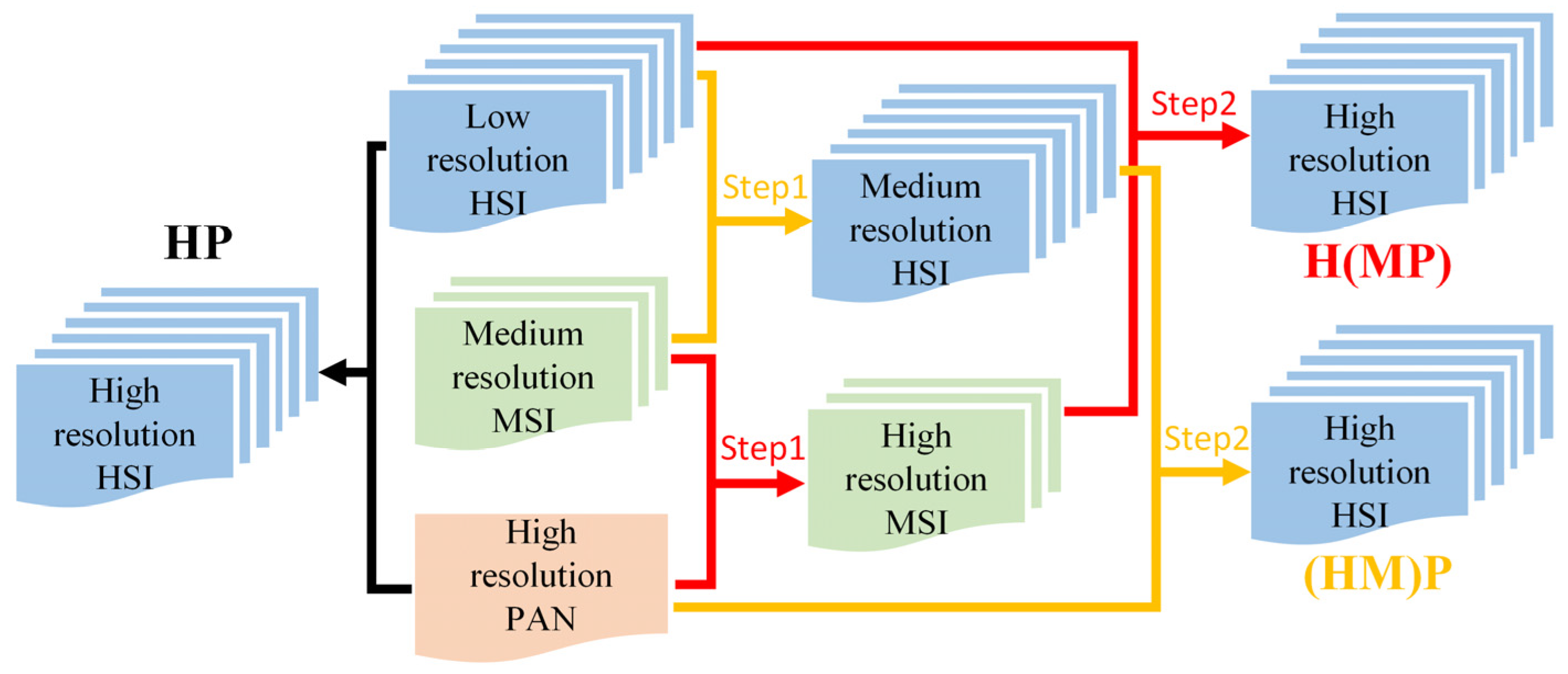
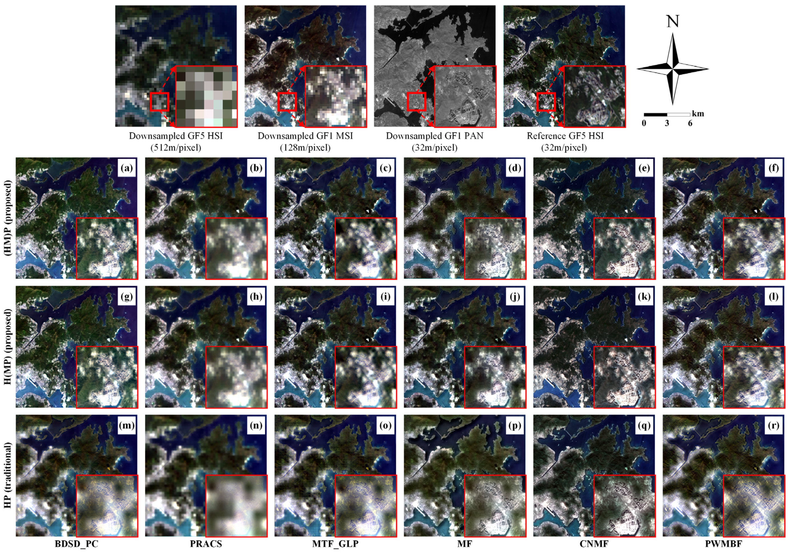
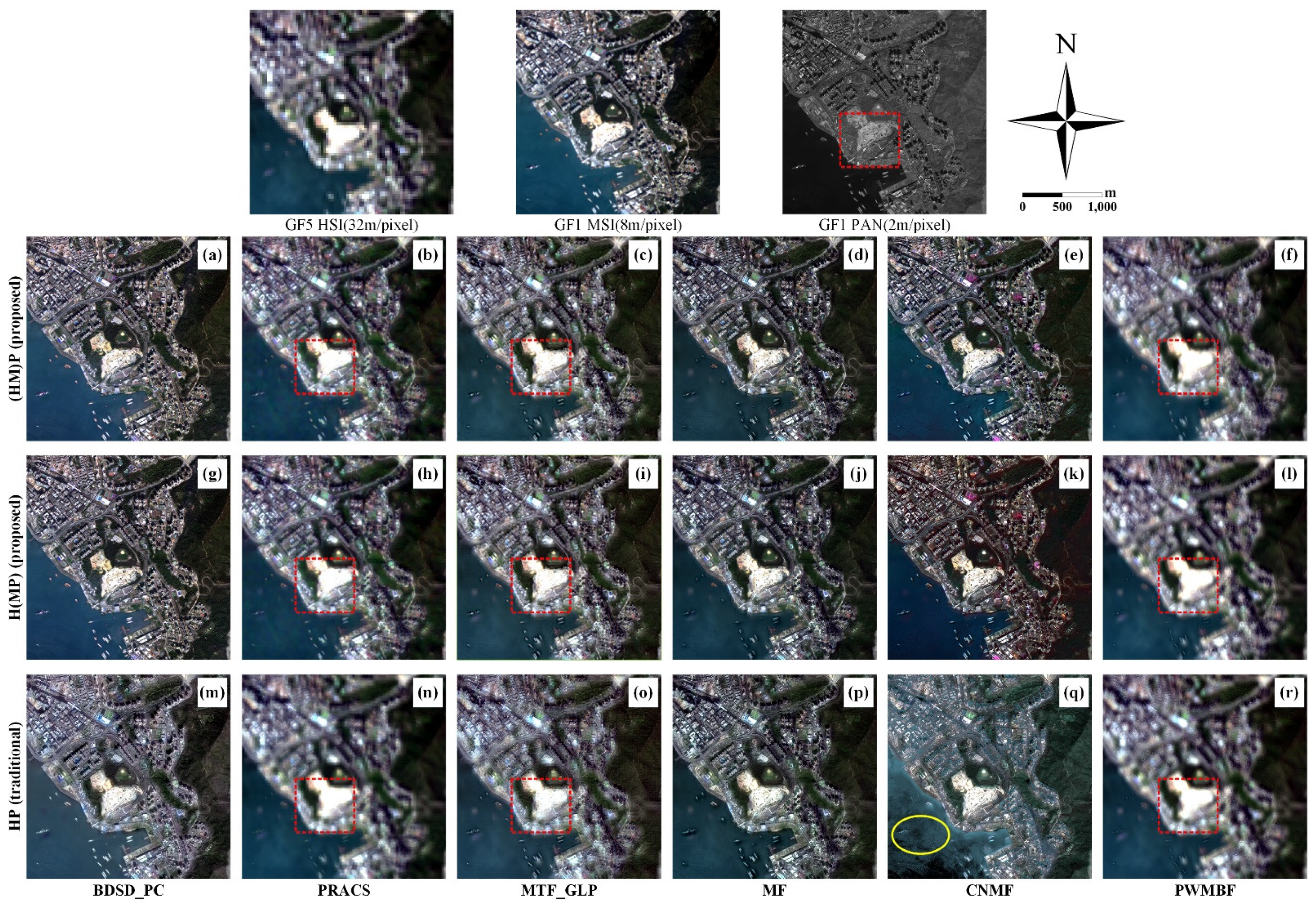
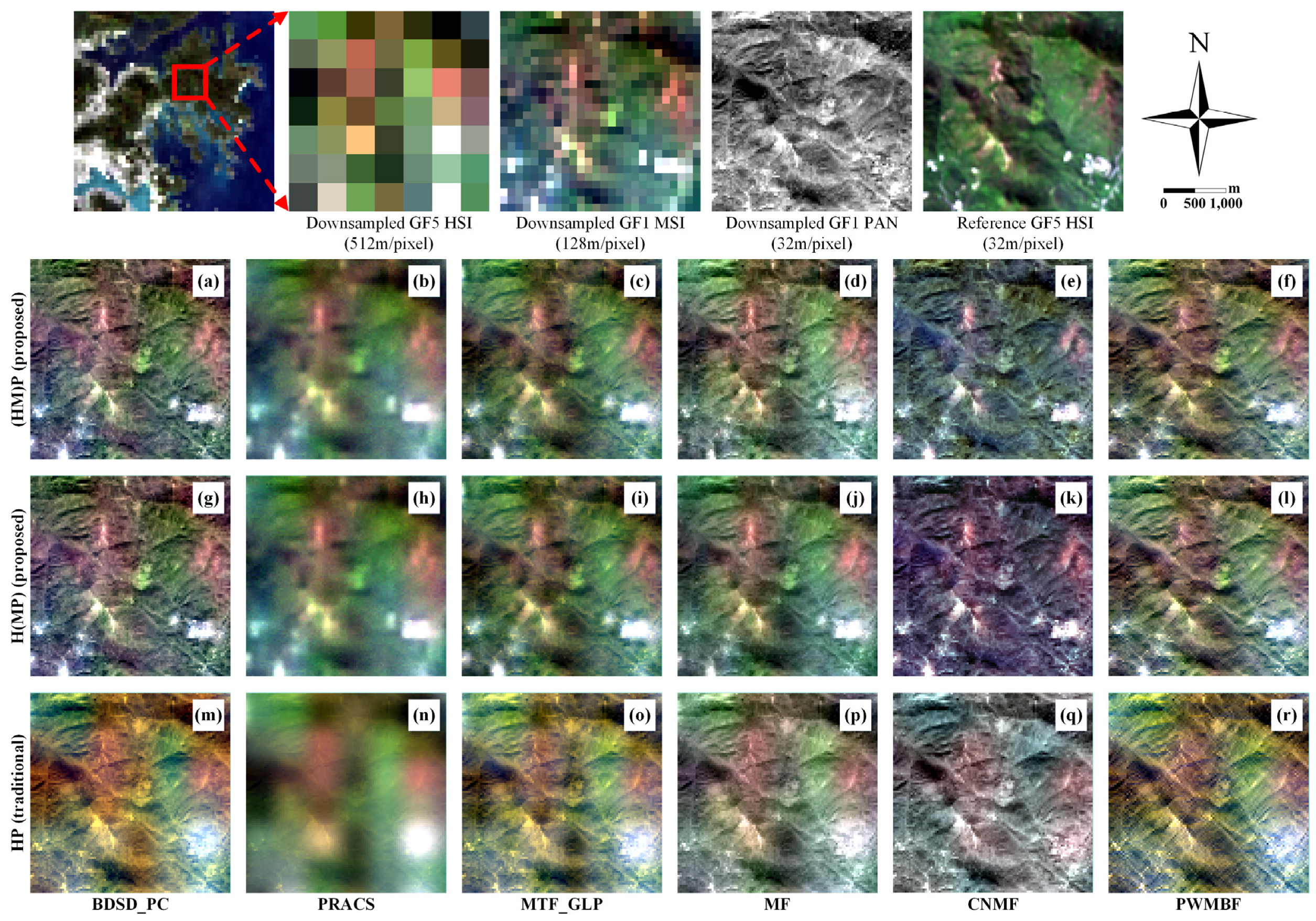
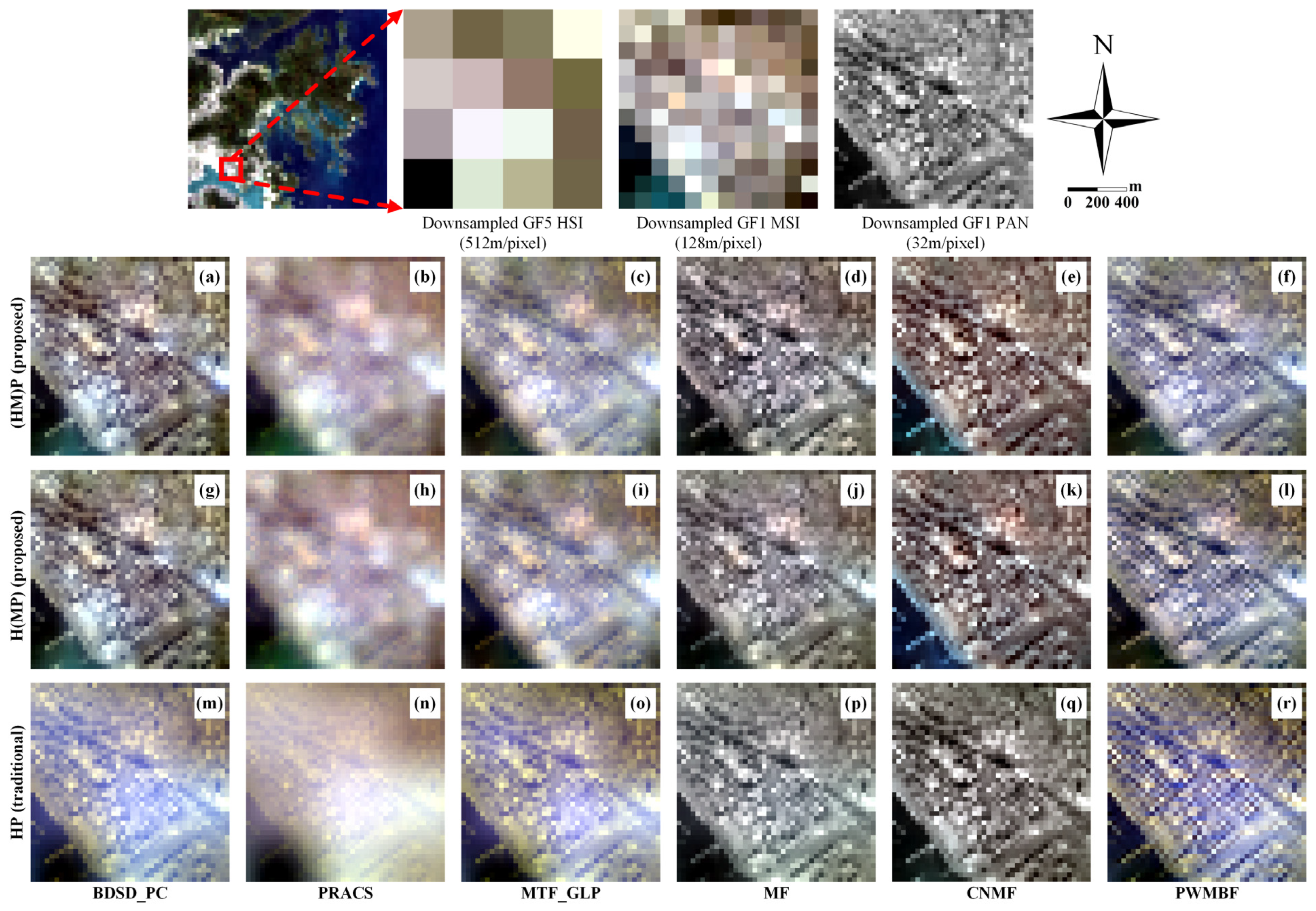
5.1. Comparison of Strategies (HM)P, H(MP) and HP

Spectral fidelity: Generally, the spectral fidelity performance using the proposed strategies (HM)P and H(MP) was better than that of strategy HP. This is because MSI acted as a bridge, which enabled better integration of spectral information. It also illustrated the effectiveness of the stepwise and spectral grouping approach.

Spatial fidelity: From the perspective of spatial fidelity, the stepwise approach was not always better than the traditional strategy. In some cases, it was even slightly worse than the traditional HP approach. Nevertheless, combining all the experimental results, we still found that the stepwise strategies were significantly better than the traditional one.

Computational efficiency: In most circumstances, the efficiency of strategy HP was better than that of strategies (HM)P and H(MP), but there was not much difference, which may be due to the fact that (HM)P and H(MP) fuse one more image than HP. However, when using CS-based algorithms, we founnd that H(MP) was more efficient than HP and (HM)P, indicating that the stepwise fusion strategy may reduce the time complexity of the CS-based methods. In most cases, the efficiency of strategy H(MP) was better than that of strategy (HM)P.

Summary: Considering the spectral and spatial fidelity comprehensively, we found that the stepwise approaches are better than traditional one. Moreover, the stepwise fusion approach did not significantly increase the time complexity compared to traditional methods, and strategy H(MP) reduced the time complexity compared to HP when using CS-based algorithms (BDSD_PC and PRACS). We also found from the experimental results that the two stepwise approaches always produce comparable results for most algorithms and images. Therefore, we suggest fusing HSI, MSI and PAN images using stepwise and spectral grouping strategies to obtain better results.

5.2. Comparison of Fusion Algorithms Using Stepwise and Spectral Grouping Strategy

In order to compare different algorithms more concisely, we qualitatively classified the performances into three levels: Good (G), Acceptable (A) and Poor (P). In this section, the performances presented in Section 4 are collected and quantified into G, A or P. As we discussed in Section 5.1, the proposed stepwise strategies outperformed the traditional HP strategy in spectral and spatial fidelity, therefore, the HP strategy is ignored in this section. Because the strategies (HM)P and H(MP) have comparable performance, we only count the performance of (HM)P and H(MP) once. The performances of different algorithms’ spectral and spatial fidelity over different images and scenes were quantified and presented in

Table 16. Quantified performances of different algorithms’ spectral and spatial fidelity (G: good, A: acceptable, P: poor).

Scenes	Images	Figure/Table	BDSD_PC	PRACS	MTF_GLP	MF	CNMF	PWMBF
Full Image (Spectral/Spatial)	Simulated	Figure 5/Table 4, Table 5, Table 6 and Table 7	P/A	G/P	G/A	G/G	G/G	G/A
	Real	Figure 6/Table 9	G/G	G/P	G/A	G/G	A/G	G/P
Vegetation Area (Spectral)	Simulated	Figure 7/Table 11, Table 12 and Table 13	P	G	G	G	P	G
	Real	Figure 8	G	G	G	G	P	G
Built-up Area (Spatial)	Simulated	Figure 9/Table 14	A	P	A	G	G	A
	Real	Figure 10/Table 15	G	P	A	G	G	P
Overall Score			P	P	A	G	P	P

. Besides, to evaluate the overall performances of different algorithms, the worst scores over different scenes and images were used, as presented in the last row of the table.

Spectral and spatial fidelity: It can be seen from Table 16, that the MF algorithm had good performance in terms of spectral and spatial fidelity for different images and scenes. The MTF_GLP algorithms performed slightly worse than MF for some areas and images. However, the worst scores of MTF_GLP methods were As, therefore, their final scores were A. The other four algorithms had some obvious defects in spectral or spatial fidelity, making them obtain poor scores, and finally resulting in the scores of P.

Computational efficiency: As can be seen from Section 4.2, from an algorithmic point of view, the computational efficiency of simulated data fusion is ranked as PWMBF > MF > MTF_GLP > BDSD_PC > CNMF > PRACS, and the computational efficiency of real data fusion is ranked as PWMBF > MF > BDSD_PC > MTF_GLP > CNMF > PRACS, so the calculation efficiency of the six algorithms can also be divided into three levels in the

Table 17. Quantified performances of computational efficiency (G: good, A: acceptable, P: poor).

Scenes	Image	Figure/Table	BDSD_PC	PRACS	MTF_GLP	MF	CNMF	PWMBF
Full Image (time complexity)	Simulated	Figure 5 Table 8	A	P	A	G	P	G
	Real	Figure 6 Table 10	A	P	A	G	P	G
Overall Score			A	P	A	G	P	G

. As is showed in Table 17, in terms of computational efficiency of the algorithms, MF and PWMBF are good, BDSD_PC and MTF_GLP are acceptable, and PRACS and CNMF are poor. From the perspective of the types of fusion algorithms, the CS-based algorithms have the lowest computational efficiency in general, while the MRA-based and subspace-based algorithms have better and equivalent computational efficiency.

It should be noted that the comparison of the algorithms is different from some other studies. We aim to evaluate the performances of these algorithms in fusing HSI, MSI and PAN images, while other comparative analyses are generally focused on their performances fusing two images [11,36]. Performance in fusing images with contrasting spectral-spatial resolutions has rarely been considered in previous studies [26].

Generally, by comparing the spectral fidelity, spatial fidelity and computational efficiency of the algorithms, we recommend the MF algorithm to fuse HSI, MSI and PAN image using a stepwise and spectral grouping strategy. In some cases, the MTF_GLP algorithms is potential candidate.

5.3. Issues to Be Further Investigated

The approach in this study has some aspects to further investigated:

(1) According to the spectral correspondence, there are only 77 bands where the spectra of GF-5 HSI and GF-1 MSI overlap. To improve the spatial resolution of HSI channels that cannot be covered by the MSI spectrum, the ratio image-based spectral resampling (RIBSR) [15] might be a solution.

(2) The stepwise fusion approach is prone to generate error accumulation, including spatial distortions and spectral errors. For spatial errors, it is necessary to perform high-precision registration of multi-source images during data preprocessing. As for spectral distortions, the quantitative evaluation indices between the fused image and the original HSI can be calculated after stepwise fusion to quantify the spectral distortions, and the error compensation mechanism can be used to eliminate the error [27].

(3) This study is instructive for sensor design, specifically, the design of an imaging system that integrates panchromatic, multispectral and hyperspectral sensors. However, when the spatial resolution of hyperspectral images and panchromatic images is determined, the optimal spatial resolutions of the MSI that can maximize the quality of fused images is still an issue that needs to be investigated in the future.

6. Conclusions

In this study, we have demonstrated the effectiveness of fusing HSI, MSI and PAN images using a stepwise and spectral grouping strategy. Two stepwise strategies were compared with a traditional one-step fusion strategy, and six state-of-the-art image fusion algorithms were adopted and compared. From this study, we can draw the following conclusions:

(1) Image fusion performances of different strategies: Compared with the traditional fusion strategy HP, the results of the stepwise fusion strategy (HM)P and H(MP) have better spectral fidelity. However, from the perspective of spatial fidelity, the strategies (HM)P and H(MP) do not always outperform the strategy HP. Nevertheless, considering all the experimental results, we still found that the stepwise strategies were better than the traditional one, while the spectral and spatial fidelity of the stepwise strategies (HM)P and H(MP) were comparable.

(2) Image fusion performances of different algorithms: Six algorithms are evaluated with the stepwise fusion strategy. The spectral and spatial fidelity of the results of the MF algorithm was the best, followed by MTF-GLP. Although the results of BDSD_PC and CNMF had good spatial fidelity, the spectral fidelity was poor, whilst PRACS and PWMBF had better spectral fidelity and poor spatial retention.

(3) Computational efficiencyof the fusion strategies: The stepwise strategy does not significantly increase the computational load when it fuses one more image than HP, and stepwise strategy H(MP) reduces the time complexity compared with HP when using CS-based algorithms. Under most algorithms, strategy H(MP) is more computationally efficient than strategy (HM)P.

(4) Computational efficiency of the fusion algorithms: From the algorithm point of view, PWMBF and MF have the highest computational efficiency, followed by MTF_GLP, BDSD_PC, and the worst is CNMF, PRACS. From the perspective of the types of fusion algorithms, the CS-based algorithms have the lowest computational efficiency in general, while the MRA and subspace-based algorithms have better and equivalent computational efficiency.

The stepwise approach is proposed from a macro perspective, so that it is not limited to specific fusion algorithms. Moreover, we have tested and compared six well-known algorithms. The results provide us with a reference for selecting an image fusion algorithm. This study has also inspired some new ideas for designing new sensor systems, such as new satellite or drone platforms carrying sensors with different spatial and spectral resolutions.

References

1. Liu, Y.-N.; Sun, D.-X.; Hu, X.-N.; Ye, X.; Li, Y.-D.; Liu, S.-F.; Cao, K.-Q.; Chai, M.-Y.; Zhou, W.-Y.-N.; Zhang, J.; et al. The Advanced Hyperspectral Imager Aboard China’s GaoFen-5 satellite. IEEE Geosci. Remote Sens. Mag. 2019, 7, 23–32. [Google Scholar] [CrossRef]
2. Grohnfeldt, C.; Zhu, X.X.; Bamler, R. Splitting the Hyperspectral-Multispectral Image Fusion Problem Autonomously into Weighted Pan-Sharpening Tasks-The Spectral Grouping Concept. In Proceedings of the 7th Workshop on Hyperspectral Image and Signal Processing—Evolution in Remote Sensing (WHISPERS), Tokyo, Japan, 2–5 June 2015. [Google Scholar]
3. Yang, D.; Luo, Y.; Zeng, Y.; Si, F.; Xi, L.; Zhou, H.; Liu, W. Tropospheric NO2 Pollution Monitoring with the GF-5 Satellite Environmental Trace Gases Monitoring Instrument over the North China Plain during Winter 2018–2019. Atmosphere 2021, 12, 398. [Google Scholar] [CrossRef]
4. Tang, B.-H. Nonlinear Split-Window Algorithms for Estimating Land and Sea Surface Temperatures From Simulated Chinese Gaofen-5 Satellite Data. IEEE Trans. Geosci. Remote Sens. 2018, 56, 6280–6289. [Google Scholar] [CrossRef]
5. Ye, X.; Ren, H.; Liu, R.; Qin, Q.; Liu, Y.; Dong, J. Land Surface Temperature Estimate From Chinese Gaofen-5 Satellite Data Using Split-Window Algorithm. IEEE Trans. Geosci. Remote Sens. 2017, 55, 5877–5888. [Google Scholar] [CrossRef]
6. Wang, F.; Gao, J.; Zha, Y. Hyperspectral sensing of heavy metals in soil and vegetation: Feasibility and challenges. Isprs J. Photogramm. Remote Sens. 2018, 136, 73–84. [Google Scholar] [CrossRef]
7. Giardino, C.; Brando, V.E.; Dekker, A.G.; Strombeck, N.; Candiani, G. Assessment of water quality in Lake Garda (Italy) using Hyperion. Remote Sens. Environ. 2007, 109, 183–195. [Google Scholar] [CrossRef]
8. Xia, J.S.; Du, P.J.; He, X.Y.; Chanussot, J. Hyperspectral Remote Sensing Image Classification Based on Rotation Forest. IEEE Geosci. Remote Sens. Lett. 2014, 11, 239–243. [Google Scholar] [CrossRef] [Green Version]
9. Demir, B.; Erturk, S. Hyperspectral image classification using relevance vector machines. IEEE Geosci. Remote Sens. Lett. 2007, 4, 586–590. [Google Scholar] [CrossRef]
10. Ye, B.; Tian, S.; Cheng, Q.; Ge, Y. Application of Lithological Mapping Based on Advanced Hyperspectral Imager (AHSI) Imagery Onboard Gaofen-5 (GF-5) Satellite. Remote Sens. 2020, 12, 3990. [Google Scholar] [CrossRef]
11. Vivone, G.; Alparone, L.; Chanussot, J.; Dalla Mura, M.; Garzelli, A.; Licciardi, G.A.; Restaino, R.; Wald, L. A Critical Comparison Among Pansharpening Algorithms. IEEE Trans. Geosci. Remote Sens. 2015, 53, 2565–2586. [Google Scholar] [CrossRef]
12. Hardie, R.C.; Eismann, M.T.; Wilson, G.L. MAP estimation for hyperspectral image resolution enhancement using an auxiliary sensor. IEEE Trans. Image Process. 2004, 13, 1174–1184. [Google Scholar] [CrossRef] [PubMed]
13. Palsson, F.; Sveinsson, J.R.; Ulfarsson, M.O. Multispectral and Hyperspectral Image Fusion Using a 3-D-Convolutional Neural Network. IEEE Geosci. Remote Sens. Lett. 2017, 14, 639–643. [Google Scholar] [CrossRef] [Green Version]
14. Wei, Q.; Bioucas-Dias, J.; Dobigeon, N.; Tourneret, J.-Y. Hyperspectral and Multispectral Image Fusion Based on a Sparse Representation. IEEE Trans. Geosci. Remote Sens. 2015, 53, 3658–3668. [Google Scholar] [CrossRef] [Green Version]
15. Chen, Z.; Pu, H.; Wang, B.; Jiang, G.-M. Fusion of Hyperspectral and Multispectral Images: A Novel Framework Based on Generalization of Pan-Sharpening Methods. IEEE Geosci. Remote Sens. Lett. 2014, 11, 1418–1422. [Google Scholar] [CrossRef]
16. Selva, M.; Aiazzi, B.; Butera, F.; Chiarantini, L.; Baronti, S. Hyper-Sharpening: A First Approach on SIM-GA Data. IEEE J. Sel. Top. Appl. Earth Obs. Remote Sens. 2015, 8, 3008–3024. [Google Scholar] [CrossRef]
17. Simoes, M.; Bioucas-Dias, J.; Almeida, L.B.; Chanussot, J. A Convex Formulation for Hyperspectral Image Superresolution via Subspace-Based Regularization. IEEE Trans. Geosci. Remote Sens. 2015, 53, 3373–3388. [Google Scholar] [CrossRef] [Green Version]
18. Zhang, Y.; De Backer, S.; Scheunders, P. Noise-Resistant Wavelet-Based Bayesian Fusion of Multispectral and Hyperspectral Images. IEEE Trans. Geosci. Remote Sens. 2009, 47, 3834–3843. [Google Scholar] [CrossRef]
19. Lanaras, C.; Baltsavias, E.; Schindler, K. Hyperspectral Super-Resolution by Coupled Spectral Unmixing. In Proceedings of the IEEE International Conference on Computer Vision, Santiago, Chile, 11–18 December 2015; pp. 3586–3594. [Google Scholar]
20. Bieniarz, J.; Mueller, R.; Zhu, X.X.; Reinartz, P. Hyperspectral Image Resolution Enhancement Based on Joint Sparsity Spectral Unmixing. In Proceedings of the IEEE Joint International Geoscience and Remote Sensing Symposium (IGARSS)/35th Canadian Symposium on Remote Sensing, Quebec City, QC, Canada, 13–18 July 2014; pp. 2645–2648. [Google Scholar]
21. Yokoya, N.; Yairi, T.; Iwasaki, A. Coupled Nonnegative Matrix Factorization Unmixing for Hyperspectral and Multispectral Data Fusion. IEEE Trans. Geosci. Remote Sens. 2012, 50, 528–537. [Google Scholar] [CrossRef]
22. Qu, J.H.; Lei, J.; Li, Y.S.; Dong, W.Q.; Zeng, Z.Y.; Chen, D.Y. Structure Tensor-Based Algorithm for Hyperspectral and Panchromatic Images Fusion. Remote Sens. 2018, 10, 373. [Google Scholar] [CrossRef] [Green Version]
23. Cetin, M.; Musaoglu, N. Merging hyperspectral and panchromatic image data: Qualitative and quantitative analysis. Int. J. Remote Sens. 2009, 30, 1779–1804. [Google Scholar] [CrossRef]
24. Qu, J.H.; Li, Y.S.; Du, Q.; Xia, H.M. Hyperspectral and Panchromatic Image Fusion via Adaptive Tensor and Multi-Scale Retinex Algorithm. IEEE Access 2020, 8, 30522–30532. [Google Scholar] [CrossRef]
25. Dong, W.; Xiao, S.; Liang, J.; Qu, J. Fusion of hyperspectral and panchromatic images using structure tensor and matting model. Neurocomputing 2020, 399, 237–246. [Google Scholar] [CrossRef]
26. Bioucas-Dias, J.M.; Plaza, A.; Camps-Valls, G.; Scheunders, P.; Nasrabadi, N.M.; Chanussot, J. Hyperspectral Remote Sensing Data Analysis and Future Challenges. IEEE Geosci. Remote Sens. Mag. 2013, 1, 6–36. [Google Scholar] [CrossRef] [Green Version]
27. Meng, X.; Sun, W.; Ren, K.; Yang, G.; Shao, F.; Fu, R. Spatial-spectral fusion of GF-5/GF-1 remote sensing images based on multiresolution analysis. J. Remote Sens. 2020, 24, 379–387. [Google Scholar]
28. Shen, H. Integrated Fusion Method for Multiple Temporal-Spatial-Spectral Images. In Proceedings of the 22nd Congress of the International-Society-for-Photogrammetry-and-Remote-Sensing, Melbourne, Australia, 25 August–1 September 2012; pp. 407–410. [Google Scholar]
29. Zhong, Y.; Wang, X.; Wang, S.; Zhang, L. Advances in spaceborne hyperspectral remote sensing in China. Geo-Spatial Inf. Sci. 2021, 24, 95–120. [Google Scholar] [CrossRef]
30. Li, J.; Feng, L.; Pang, X.P.; Gong, W.S.; Zhao, X. Radiometric cross Calibration of Gaofen-1 WFV Cameras Using Landsat-8 OLI Images: A Simple Image-Based Method. Remote Sens. 2016, 8, 411. [Google Scholar] [CrossRef] [Green Version]
31. Hao, P.; Wang, L.; Niu, Z. Potential of multitemporal Gaofen-1 panchromatic/multispectral images for crop classification: Case study in Xinjiang Uygur Autonomous Region, China. J. Appl. Remote Sens. 2015, 9, 096035. [Google Scholar] [CrossRef]
32. Mookambiga, A.; Gomathi, V. Comprehensive review on fusion techniques for spatial information enhancement in hyperspectral imagery. Multidimens. Syst. Signal Process. 2016, 27, 863–889. [Google Scholar] [CrossRef]
33. Li, X.; Yuan, Y.; Wang, Q. Hyperspectral and Multispectral Image Fusion Based on Band Simulation. IEEE Geosci. Remote Sens. Lett. 2020, 17, 479–483. [Google Scholar] [CrossRef]
34. Luo, S.; Zhou, S.; Qiang, B. A novel adaptive fast IHS transform fusion method driven by regional spectral characteristics for Gaofen-2 imagery. Int. J. Remote Sens. 2020, 41, 1321–1337. [Google Scholar] [CrossRef]
35. Ren, K.; Sun, W.; Meng, X.; Yang, G.; Du, Q. Fusing China GF-5 Hyperspectral Data with GF-1, GF-2 and Sentinel-2A Multispectral Data: Which Methods Should Be Used? Remote Sens. 2020, 12, 882. [Google Scholar] [CrossRef] [Green Version]
36. Yokoya, N.; Grohnfeldt, C.; Chanussot, J. Hyperspectral and Multispectral Data Fusion A comparative review of the recent literature. IEEE Geosci. Remote Sens. Mag. 2017, 5, 29–56. [Google Scholar] [CrossRef]
37. Vivone, G. Robust Band-Dependent Spatial-Detail Approaches for Panchromatic Sharpening. IEEE Trans. Geosci. Remote Sens. 2019, 57, 6421–6433. [Google Scholar] [CrossRef]
38. Choi, J.; Yu, K.; Kim, Y. A New Adaptive Component-Substitution-Based Satellite Image Fusion by Using Partial Replacement. IEEE Trans. Geosci. Remote Sens. 2011, 49, 295–309. [Google Scholar] [CrossRef]
39. Aiazzi, B.; Alparone, L.; Baronti, S.; Garzelli, A.; Selva, M. MTF-tailored multiscale fusion of high-resolution MS and pan imagery. Photogramm. Eng. Remote Sens. 2006, 72, 591–596. [Google Scholar] [CrossRef]
40. Restaino, R.; Vivone, G.; Dalla Mura, M.; Chanussot, J. Fusion of Multispectral and Panchromatic Images Based on Morphological Operators. IEEE Trans. Image Process. 2016, 25, 2882–2895. [Google Scholar] [CrossRef] [Green Version]
41. Palsson, F.; Sveinsson, J.R.; Ulfarsson, M.O.; Benediktsson, J.A. Model-Based Fusion of Multi-and Hyperspectral Images Using PCA and Wavelets. IEEE Trans. Geosci. Remote Sens. 2015, 53, 2652–2663. [Google Scholar] [CrossRef]
42. Ghassemian, H. A review of remote sensing image fusion methods. Inf. Fusion 2016, 32, 75–89. [Google Scholar] [CrossRef]
43. Garzelli, A.; Nencini, F.; Capobianco, L. Optimal MMSE pan sharpening of very high resolution multispectral images. IEEE Trans. Geosci. Remote Sens. 2008, 46, 228–236. [Google Scholar] [CrossRef]
44. Vivone, G.; Dalla Mura, M.; Garzelli, A.; Restaino, R.; Scarpa, G.; Ulfarsson, M.O.; Alparone, L.; Chanussot, J. A New Benchmark Based on Recent Advances in Multispectral Pansharpening: Revisiting Pansharpening With Classical and Emerging Pansharpening Methods. IEEE Geosci. Remote Sens. Mag. 2021, 9, 53–81. [Google Scholar] [CrossRef]
45. Lee, D.D.; Seung, H.S. Learning the parts of objects by non-negative matrix factorization. Nature 1999, 401, 788–791. [Google Scholar] [CrossRef] [PubMed]
46. Loncan, L.; Almeida, L.B.; Bioucas-Dias, J.M.; Briottet, X.; Chanussot, J.; Dobigeon, N.; Fabre, S.; Liao, W.; Licciardi, G.A.; Simoes, M.; et al. Hyperspectral Pansharpening: A Review. IEEE Geosci. Remote Sens. Mag. 2015, 3, 27–46. [Google Scholar] [CrossRef] [Green Version]
47. Alparone, L.; Wald, L.; Chanussot, J.; Thomas, C.; Gamba, P.; Bruce, L.M. Comparison of pansharpening algorithms: Outcome of the 2006 GRS-S data-fusion contest. IEEE Trans. Geosci. Remote Sens. 2007, 45, 3012–3021. [Google Scholar] [CrossRef] [Green Version]
48. Ranchin, T.; Wald, L. Fusion of high spatial and spectral resolution images: The ARSIS concept and its implementation. Photogramm. Eng. Remote Sens. 2000, 66, 49–61. [Google Scholar]
49. Wald, L.; Ranchin, T.; Mangolini, M. Fusion of satellite images of different spatial resolutions: Assessing the quality of resulting images. Photogramm. Eng. Remote Sens. 1997, 63, 691–699. [Google Scholar]
Figure 1. Geographical location of study area. On the right is the 30 m GF-5 HSI with true color display (R: 639 nm; G: 549 nm; B: 472 nm).
Remotesensing 14 01021 g001
Figure 2. Spectral correspondences between hyperspectral image and multispectral image.
Remotesensing 14 01021 g002
Figure 3. Spectral Grouping fusion framework.
Remotesensing 14 01021 g003
Figure 4. Flowchart of three different fusion strategies. The yellow, red, and black arrows indicate the steps of three different strategies, respectively.
Remotesensing 14 01021 g004
Figure 5. (ar) Fusion results of simulated GF5 and GF1 images.
Remotesensing 14 01021 g005
Figure 6. (ar) Fusion results of real GF5 and GF1 images. Some poor results are marked in the figures.
Remotesensing 14 01021 g006
Figure 7. (ar) Vegetation areas of simulated images fusion.
Remotesensing 14 01021 g007
Figure 8. (ar) Vegetation areas of real GF5 and GF1 images fusion.
Remotesensing 14 01021 g008
Figure 9. (ar) Build-up area simulated image fusion.
Remotesensing 14 01021 g009
Figure 10. (ar) Build-up area, real GF5 and GF1 images fusion.
Remotesensing 14 01021 g010