Abstract
The utility of unmanned aerial vehicles (UAV) imagery in retrieving phenotypic data to support plant breeding research has been a topic of increasing interest in recent years. The advantages of image-based phenotyping are related to the high spatial and temporal resolution of the retrieved data and the non-destructive and rapid method of data acquisition. This study trains parametric and nonparametric regression models to retrieve leaf area index (LAI), fraction of absorbed photosynthetically active radiation (fAPAR), fractional vegetation cover (fCover), leaf chlorophyll content (LCC), canopy chlorophyll content (CCC), and grain yield (GY) of winter durum wheat breeding experiment from four-bands UAV images. A ground dataset, collected during two field campaigns and complemented with data from a previous study, is used for model development. The dataset is split at random into two parts, one for training and one for testing the models. The tested parametric models use the vegetation index formula and parametric functions. The tested nonparametric models are partial least square regression (PLSR), random forest regression (RFR), support vector regression (SVR), kernel ridge regression (KRR), and Gaussian processes regression (GPR). The retrieved biophysical variables along with traditional phenotypic traits (plant height, yield, and tillering) are analysed for detection of genetic diversity, proximity, and similarity in the studied genotypes. Analysis of variance (ANOVA), Duncan’s multiple range test, correlation analysis, and principal component analysis (PCA) are performed with the phenotypic traits. The parametric and nonparametric models show close results for GY retrieval, with parametric models indicating slightly higher accuracy (R2 = 0.49; RMSE = 0.58 kg/plot; rRMSE = 6.1%). However, the nonparametric model, GPR, computes per pixel uncertainty estimation, making it more appealing for operational use. Furthermore, our results demonstrate that grain filling was better than flowering phenological stage to predict GY. The nonparametric models show better results for biophysical variables retrieval, with GPR presenting the highest prediction performance. Nonetheless, robust models are found only for LAI (R2 = 0.48; RMSE = 0.64; rRMSE = 13.5%) and LCC (R2 = 0.49; RMSE = 31.57 mg m−2; rRMSE = 6.4%) and therefore these are the only remotely sensed phenotypic traits included in the statistical analysis for preliminary assessment of wheat productivity. The results from ANOVA and PCA illustrate that the retrieved remotely sensed phenotypic traits are a valuable addition to the traditional phenotypic traits for plant breeding studies. We believe that these preliminary results could speed up crop improvement programs; however, stronger interdisciplinary research is still needed, as well as uncertainty estimation of the remotely sensed phenotypic traits.
1. Introduction
Yield is a major quantitative trait formed in a complex manner by all other traits related to productivity. It is a leading feature in breeding programs and its improvement is a major task that requires high-throughput phenotyping platforms. From the point of view of plant breeding, yield per unit area is of considerable importance [1,2] and the primary goal is to expand genetic diversity and develop new cultivars that perform better than those grown in the target population of environments. Traditionally, breeders search for genetic variation among winter durum wheat (Triticum turgidum L. var. durum) parents to derive superior progeny from crossing and selection [1]. To meet this goal, high-throughput field-phenotyping tools are needed [3]. Field phenotyping in plant breeding measures small plots with limited resources available and time required for the measurements, considering the quality of the acquired data and data analysis. Even if field-based high-throughput phenotyping platforms remain a barrier for future breeding advances [4,5,6], the existing relatively low-cost sensors and unmanned aerial vehicles (UAVs) provide possibilities for producing extensive amounts of georeferenced data. Whilst challenging to manage, such large datasets also offer opportunities for applying new modelling techniques, such as machine learning [7] and increasing selection intensity, improving selection accuracy, and improving the decision support system.
In recent years, a multitude of studies [4,8,9,10] have reviewed the platforms, sensors, and applications for remote sensing technologies for field crop phenotyping. Today’s consensus [11,12] is that UAVs can provide the spatial and temporal resolution needed for high-throughput phenotyping of crops, thus addressing a current bottleneck in the selection of superior genotypes in breeding and variety development programs. Plant phenotypic traits are determined by genetic and environmental factors and the interaction between them. The most studied [8] phenotypic traits in breeding programs are yield, biomass, height, leaf area index (LAI), chlorophyll, nitrogen, and diseases. Phenotypic traits are measured directly or retrieved using RGB, multispectral, hyperspectral, thermal, and LiDAR sensors. However, the price for those different sensors is not the same and the effort it takes to analyse the data is also very different. Still under development are data-processing algorithms or tools [4] to convert the remotely sensed data into useful phenotyping data for variety selection and plant growth in general.
Most wheat breeding programs rely on vegetation indices (VI) for the estimation of grain yield and phenotypic traits. Different sensors mounted on UAV platforms have been operated in the last ten years to collect remote sensing data in field-scale wheat trials. Studies focused on assessing disease severity [13], the genotypic performance of durum wheat under a wide range of growing conditions at four different phenological stages with RGB, multispectral, hyperspectral, and thermal UAV sensors [14], and retrieving plant height [15] from RGB UAV 3D digital surface models of crop field trials produced via structure from motion (SfM) that shows growth rate. Many studies rely on VI to detect with success senescence’s dynamic in bread wheat with normalised difference red-edge index (NDREI) [16] in order to predict grain yield with NDVI [17] or GNDVI recorded at early reproductive stages [18] or with hyperspectral VI (R810/R560) combined with plant height and retrieved with linear nonparametric model (PLSR) [19].
Maize is another crop that is widely studied in plant phenotyping. Different studies estimated maize yield from VI obtained from RGB camera, mounted on a UAV [20]; biomass, with RGB camera, mounted on a UAV and neural networks [21]; plant-height growth and canopy spectral dynamics [22], LAI with the coupled PROSPECT and SAIL radiative transfer models (PROSAIL) [23]. Disease in maize was studied with disease-resistant classification, with UAV VI [24], or with computer vision modelling based on neural network and UAV data [25].
Studies on other crops, like barley, have found that UAV VIs can significantly separate best and least performing genotypes [26] or that nitrogen use efficiency [27] can be assessed with RGB and multispectral UAV VIs and thermal data. In sugar beet, LAI, leaf, and canopy chlorophyll contents are retrieved with VIs and PROSAIL inversion approaches [28]. The study concluded that, providing that enough samples are included in the calibration set, VIs provide slightly more accurate performances than PROSAIL inversion. Computer vision models based on neural network and UAV data are successfully developed for panicle detection in rice phenotyping experiments [29].
Instead of directly using the spectral bands to train nonparametric regression models, an interesting approach is using VIs as input for nonparametric regression [30,31,32]. In this case, the features are either retrieved by applying VIs and then the output of the best performing parametric models is fed as an input to the nonparametric models, or just by choosing one index, for example, NDVI. This method is applied to retrieving soybean yield from UAV multispectral sensors, RGB, multispectral and thermal [30], UAV hyperspectral sensor [32], and wheat yield from satellite NDVI [31] with high accuracy.
Biophysical variables and crop yield are traits of great interest to breeders since they are directly related to crop productivity. They are often used as crop phenotypic traits under field conditions [6]. Leaf area index, fraction of absorbed photosynthetically active radiation (fAPAR), and fractional vegetation cover (fCover) have been recognised as essential variables by the Group on Earth Observations Global Agricultural Monitoring Initiative (GEOGLAM) for the study of agriculture [33]. Chlorophyll, measured as leaf chlorophyll content (LCC) and canopy chlorophyll content (CCC), is an important photosynthetic pigment to the plant, largely determining photosynthetic capacity and hence plant growth.
When quantifying biophysical variables from remote sensing data, the retrieval methods are classified into four categories [34]: parametric, nonparametric, hybrid regression methods, and physically based methods. Parametric and nonparametric methods also apply to yield retrieval.
VIs and parametric functions are fitted to the biophysical variable or yield. Assuming empirical relationships between VIs and crop characteristics, regression has been developed for yield estimation in wheat [35] or biophysical variables retrieval [36]. Although vegetation indices are widely used, they depend only on a few available spectral bands and the full spectrum of information in the available data is not exploited. Furthermore, the VIs are created and tested with preselected bands, which makes them difficult to apply to different remote sensing data. Therefore, instead of using the published VIs, formulas of spectral bands are defined. The formulas with all available spectral bands are tested. The parametric model is constructed by fitting the parametric function to the result of the formula [37].
The nonparametric methods could be classified into linear and nonlinear [34,38]. Moreover, the nonlinear nonparametric methods are grouped into three families: kernel-based machine learning regression, neural networks, and decision tree. Many machine learning methods for yield estimation have been tested in precision agriculture [39].
Each method has its advantages and disadvantages; however, the most adopted method for crop phenotyping by UAV remote sensing is mainly the empirical statistical model [40]. The freely available toolbox, ARTMO [41], allows for a quick and easy construction of parametric and nonparametric regression models with any spectral bands. Even though the nonparametric regression algorithms are more flexible and construct the models with all available information (all remote sensing bands) and could better fit the data, the parametric regression algorithm has the major advantage of being easily understood and applied.
In the present research, our aim is: (1) to retrieve five biophysical variables of winter durum wheat, LAI, fAPAR, fCover, LCC, and CCC, with UAV multispectral data and parametric and nonparametric regression models. The biophysical variables retrieved with robust models are considered as remotely sensed phenotypic traits; (2) to statistically analyse the remotely sensed traits, in complement to traditional phenotypic traits that breeders collect, to detect genetic distance in the studied winter durum wheat genotypes. This analysis is conducted to evaluate the usefulness of the remotely sensed phenotypic traits in the breeding process as sources of information for the formation of new and highly productive wheat varieties; (3) to estimate grain yield of winter durum wheat with UAV multispectral data and parametric and nonparametric regression models at different phenophases.
2. Materials and Methods
2.1. Site (Field) and Experimental Design of the Study
The study took place in the 2020/2021 growing season on the territory of the breeding fields of the Field Crops Institute, Chirpan (FCI-Chirpan), Bulgaria (Figure 1). The genotypes were of winter durum wheat (Triticum turgidum L. var. durum) and were grown on flat terrain. The altitude varies between 208–209 m a.s.l. and the soil is classified as Pellic Vertisol, according to the World Reference Base for Soil Resources classification system [42]. The climate in the region is temperate continental, with a poorly expressed Mediterranean influence. Therefore, the conditions of the natural environment favour the growth of winter durum wheat. Meteorological conditions during the year of the study were characterised by higher temperatures than the multiannual norm (12.7% over the average). The harvest year was favourable in terms of soil moisture and rainfall higher than the average (8.5% over the average) and was suitable for obtaining a high yield (Table 1).
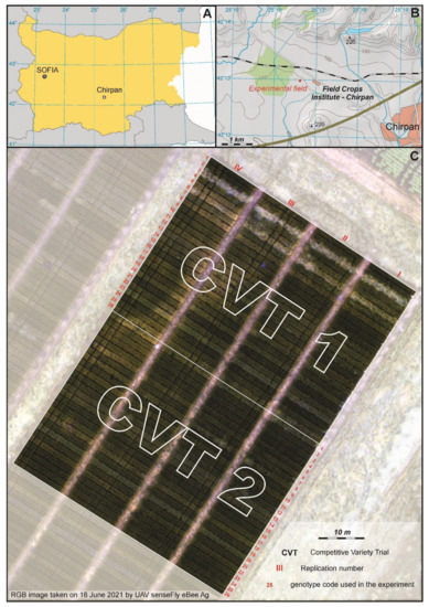
Figure 1.
Study area. (A)—Location of FCI-Chirpan in Bulgaria. (B)—Location of the breeding experimental field. (C)—Orthophoto map of the breeding experimental field divided into 208 plots and two competitive variety trials (CVTs); each CVT has 26 genotypes with 4 replicates.

Table 1.
Meteorological characteristics during the vegetation of durum wheat in FCI-Chirpan for the 2021 harvest and the average meteorological data for the multiannual period. The data are from the FCI-Chirpan weather station situated less than 500 m from the test site.
Fifty genotypes of durum wheat varieties and breeding lines grown in rainfed field conditions were distributed in two competitive variety trials (CVTs), CVT 1 and CVT 2, each of them comprising 26 genotypes. In CVT 1, 18 old and modern Bulgarian varieties and 8 newly developed breeding lines were grown and in CVT 2, there were 24 newly developed breeding lines. The varieties Predela and Mirela were sown in each trial as a standard (Table A1). The CVTs were conducted to evaluate grain yield (GY), yield-related traits, disease resistance, and grain quality in new durum wheat varieties and advanced breeding lines, created in FCI-Chirpan. The experiment was repeated over a minimum of three years. This organisation of the field experiment and statistical processing of data allow distinguishing the variation due to non-genetic factors, including field heterogeneity associated with soil differences, and reduce the error of the experiment.
The trials were organised by complete block design in four replications (Figure 1). Genotypes were sown on 05.11.2020 (CVT 1) and 06.11.2020 (CVT 2) on plots with an area of 13.2 m2 (12 × 1.10 m). The distance between the genotypes was 0.5 m and between the replications 2 m. Each genotype was sown with 550 germinated seeds per m2. The standard technology for growing durum wheat breeding materials in FCI–Chirpan was applied. The predecessor was winter peas. One-time nitrogen (N) fertilisation with fertiliser rate of 100 kg/ha of active substance nitrogen in February 2021 was applied. In addition, 92 kg/ha active substance P2O5 was applied before the sowing of durum wheat. Fertilization with N and P was carried out each year in the experimental field, based on the results of long-term fertilisation experiments in the FCI–Chirpan, and including the results of appropriate agrochemical analyses for the content of essential macro elements in soil and plants [43]. The long-term results show that the highest agronomic efficiency of nitrogen for grain and grain protein was obtained at a moderate rate of N. The agronomic efficiency of nitrogen for grain protein shifted slightly and decreased with the increase of the fertilising rate over N120 [43]. The experiment was treated against weeds with an herbicide combination of Sekator OD and Puma Super 7.5 EB. No pesticides for disease or pest control were utilised to be able to select resistant genotypes and no pathogens and pests in density above the economic threshold (ET) value were observed in the durum wheat vegetation. Brown rust, yellow rust, and leaf spot pathogens caused by fungal septoria (STB) pathogens were observed in the experiments at very low density during May and in relatively low density during June.
2.2. Data Acquisition
The most important observations and largest number of data collection in wheat breeding programs are usually conducted and collected during the principal development stages, flowering (BBCH5) and grain filling (BBCH7). Those stages under our climatic conditions occur in May and June. In this study, data from two sources have been combined, ground-measured data and data from UAV. They were obtained during the two field campaigns conducted May–June 2021 (Table A2). The field campaigns were conducted in this period because the durum wheat was in the flowering and grain filling phenological development stage, which is appropriate for forecasting the potential crop grain yield. The ground-measured data, LAI, fAPAR, fCOVER, and LСС, were collected from the trials of the first and second replication.
UAV images of the two CTVs were gained during the collection of ground-measured data. GPS data for accurate georeferencing of the UAV multispectral images were acquired as well.
2.2.1. Phenological Development Stages and Traditional Phenotypic Traits
During the field campaigns, traditional phenotypic data and ground measurements were collected (Table A2). These were as follows: phenological development stage, registered using BBCH identification keys [44,45]; plant height (cm), measured from the ground surface to the end of the spike without the awns on the main stem; number of productive tillers (tillering), measured at full maturity phenophase of the plants and just before the harvest. The data were collected from the middle of each plot, characterising the studied genotypes.
2.2.2. Grain Yield (GY)
The GY (kg/plot) was collected at the agricultural full maturity phenophase of the plants by mechanical harvesting with a classic plot combine separately for each plot on 14 July 2021 (CVT 1) and 15 July 2021 (CVT 2). The GY of a plot is obtained after weighing, with an electronic scale, the harvested grain from a plot. The GY averaged from the four replications of each genotype are described in Table A1.
2.2.3. Biophysical Variables Measured by Non-Invasive Methods
The crop’s biophysical variables, LAI, fAPAR, fCover, were measured with the instrument AccuPAR PAR/LAI Ceptometer, L.P.-80, during the two field campaigns. The parameter χ (angular leaf distribution) in the instrument was set at 0.96, which is the default value for wheat. An external sensor, assembled on a tripod and levelled, was used to record the incident radiation over the vegetation. This helps to minimise errors in cases where solar light changed quickly due to variable cloudiness. A series of above- and below-canopy measurements was used by the instrument to derive two parameters: t, which is the share of incoming radiation, let through the vegetation, and r, which is the share of incoming radiation, reflected by the vegetation (and soil) and reaching the sensor located above the vegetation. To derive t, a total of 10 measurements per plot (replication) were made and averaged, providing more representative vegetation canopy information. The fAPAR, LAI, and fCover were derived from the measured t and r, either automatically by the instrument (with LAI) or by subsequent calculations in a spreadsheet (in the case of fAPAR and fCover) (Table 2).
Table 2.
Descriptive statistics for the ground-measured biophysical variables of winter durum wheat during the two field campaigns.
Leaf chlorophyll content (LCC) was measured with the instrument CCM-300 (OPTI-SCIENCES). In the middle of the plot, four representative plants for the plot were chosen. From each plant, a measurement was made in the middle of the flag leaf blade. The four measurements per plot were averaged (Table 2). Canopy chlorophyll content (CCC) was calculated by Formula (1).
CCC = LCC × LAI
2.2.4. UAV Data Collection
To obtain multispectral images, during both field campaigns, flight missions have been carried out (Table 3) by the specialized unmanned aerial vehicle senseFly eBee Ag. The system, intended for mapping agricultural areas, includes: (1) a UAV with a fixed wing and assembled Parrot Sequoia camera with two types of sensors (Table 4), plus a sunshine (light) sensor (Parrot SA, Paris, France). In this study, the images obtained from the multispectral sensor (Table 4) were used since the sunshine sensor operated at the same (green, red, red edge, and NIR) spectral bands, and calibrated values for the object’s brightness were retrieved; (2) the eMotion 2 software which is used for planning, simulating, and controlling the flight of eBee Ag, and (3) an automated 3D processing desktop software Pix4D mapper.
Table 3.
UAV flight missions’ dates, corresponding phenological development stage of the studied genotypes of winter durum wheat, and weather condition during the flight.
Table 4.
Spectral bands for the Parrot Sequoia UAV camera.
The two flight missions were carried out while observing identical parameters: average flight height: 56 m; image-taking area: 3.7 ha; flight duration: 13 min; spatial resolution: 5 cm/pixel; image overlap forward and sideward: 80%; the number of images: 940. The sunshine sensor is used for automatic adjustment of readings to ambient light, which enables multitemporal acquisitions to be comparable.
The UAV eBee Ag has an inbuilt GPS, which provides horizontal accuracy of ~5 m. To achieve higher accuracy during the georeferencing of the UAV images, portable ground control points (GCPs) were used. The GCPs, white plastic squares sized 0.25 × 0.25 m, were laid on the four edges of CVT 1 and CVT 2 prior to the first flight mission. These were left on the ground, to be visible during the second field campaign. Using GNSS equipment Leica GS08 plus in RTK mode, the geographic coordinates were measured, achieving an accuracy of 1–3 cm.
2.2.5. Additional Data from the Zlatia Site
To cover a wider range of variations of the biophysical variables LAI, fAPAR, fCover, LCC, and CCC [46], additional data have been used (Table 5). They were obtained during three field campaigns carried out in the 2016/2017 agricultural year on six farmer fields sown with two varieties, Enola and Anapurna, of winter wheat (Triticum aestivum L.) on the territory of the Zlatia test site, Municipality of Knezha, Pleven region, Bulgaria [36,47]. These field campaigns were carried out in relation to implementing the TSAgroBG project. Several elementary sampling units (ESUs) were determined within each field, in which LAI, fAPAR, fCover, LCC, and CCC measurements were made. The fields were imaged using a UAV. The research equipment used for measuring biophysical parameters and for image acquisition was the same as the one used in this study.
Table 5.
Descriptive statistics for the biophysical variables of winter wheat crops (BBCH 22 to 26, BBCH 31 to 33, and BBCH 65 to 69) measured in the Zlatia site during three field campaigns in the agricultural year 2016/2017, n = 80.
2.3. Image Processing and Data Extraction
Initially, the multispectral images acquired during both flight missions were georeferenced by data from the onboard GPS in the coordinate system UTM zone 35 datum WGS 1984. Based on these, an orthophoto mosaic was generated for both CVTs. This study requires very high precision during the georeferencing of the orthophoto mosaic. For this purpose, additional adjustment of the georeferencing was performed by a first-order polynomial, using the GCP coordinates.
The subsequent processing of the images was carried out in GIS. This processing involves: (1) outlining elementary units (EUs): in the middle of each plot, on the orthophoto mosaic, a vector polygon sized 50 × 50 cm (100 pixels) was outlined. A vector layer was created whereas, in the attributive table, information about the geographical coordinates and code of the EUs was registered; (2) deriving data from the spectral band: the created vector layer was used to derive values for the spectral brightness of each pixel of the image falling within the boundaries of each EU. The obtained values were averaged for each EU for each of the four spectral bands. Moreover, it is consistent with ground-truth biophysical measurements that were performed. These data were used as input to parametric and nonparametric models.
2.4. Modelling and Statistical Analysis
The modelling process is summarised in Figure 2. The field and remote sensing data are the input for constructing the parametric and nonparametric models. The best model for GY retrieval is applied to present a map of GY with very high spatial resolution. The best models for biophysical variable retrieval serve as high-throughput remotely sensed phenotypic traits. The selected remotely sensed and traditional traits are analysed for detection of genetic diversity, proximity, and similarity in the studied genotypes.
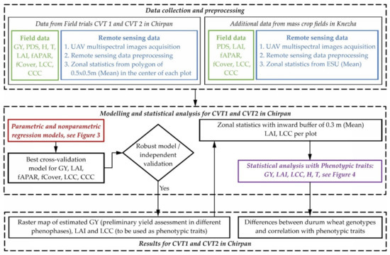
Figure 2.
Workflow diagram of phenotypic traits estimation and preliminary yield assessment in different phenophases of a wheat breeding experiment.
2.4.1. Parametric and Nonparametric Regression Models for GY and Biophysical Variables Retrieval
We used parametric and nonparametric regression algorithms to retrieve the biophysical variables and GY from UAV multispectral data. The modelling was carried out with the ARTMO toolbox [41] (https://artmotoolbox.com/, last accessed 15 February 2022) and is summarised in Figure 3.
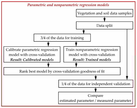
Figure 3.
Workflow diagram of the parametric and nonparametric regression modelling.
Five widely used machine-learning regression methods (partial least square regression (PLSR), random forest regression (RFR), support vector regression (SVR), kernel ridge regression (KRR), and Gaussian processes regression (GPR)) and several generic types of vegetation indices (Table 6) and parametric functions (Table 7) were tested in this study.
Combination of spectral bands (vegetation indices) is fitted to the studied variables with parametric functions. A selection of formulas, based on published VI, is provided in Table 6. The aim is to have a wide selection of formulas, including one, two, three, and four bands.
The PLSR technique [48] generalises and combines features of principal component regression (PCR) and multiple linear regression. Here, the aim of PLSR is to build a linear model. The optimal number of components in PLSR analysis is determined by minimising the prediction residual error sum of squares (PRESS) statistic. The PRESS statistic is calculated via cross-validation for each model. RFR [49] is an ensemble method based on building multiple decision trees by bootstrap sampling. It constructs a collection of decision trees with controlled variance. SVR [50], KRR [51], and GPR [52] are kernel-based methods. The kernel function used in our study is the radial basis function (RBF). SVR is based on the support vector machine (SVM) with insensitive loss as a loss function and ridge regression regularisation. KRR has an identical model form to SVR, but it uses square error loss as a loss function. GPR is based on Gaussian processes and because it is a probabilistic model, it computes uncertainty as prediction intervals of the trained model.
Previous studies have found that including bare soil samples increases the determination power of the models [12,53]. Therefore, the whole dataset for biophysical variables retrieval consisted of 307 samples (80 samples from Zlatia test site, 205 samples from Chirpan, 22 samples of bare soil from Chirpan). The dataset for GY retrieval comprised 219 samples (208 samples from Chirpan, 11 samples of bare soil from Chirpan). Before applying each method, we first randomly divided the whole dataset into two parts: three-quarters of the dataset was used for training and one-quarter for tests. The bare soil samples and those from the Zlatia test site were part of the training dataset. The test dataset contained only vegetation samples from Chirpan. Next, we determined the best hyperparameters for each model from empirical candidates based on the cross-validated coefficient of determination (R2) and root mean square error (RMSE) calculated by applying the tenfold cross-validation using only the training dataset. We applied the test dataset to the optimised models and compared the estimated and measured variables, using five metrics: R2, RMSE, normalised RMSE (nRMSE), relative RMSE (rRMSE), and Nash–Sutcliffe efficiency (NSE). The equations for these metrics are described in [54] and are the same used in the ARTMO toolbox. The goodness-of-fit metrics for the cross-validation were calculated by ARTMO toolbox and for the test dataset by scipy.stats function in Python.
Table 6.
List of the generic types of vegetation indices selected for testing in the study.
Table 6.
List of the generic types of vegetation indices selected for testing in the study.
| Name | Formula 1 | Scale | Related to | Reference |
|---|---|---|---|---|
| R | Ra | Canopy | LAI | [39] |
| Canopy | Chl | [55] | ||
| SR | Ra/Rb | Leaf & Canopy | Chl | [55] |
| Canopy | CCC, LAI | [36] | ||
| Canopy | GY prediction | [30,32] | ||
| DVI | Ra − Rb | Leaf & Canopy | Chl | [55] |
| ND | (Ra − Rb)/(Ra + Rb) | Canopy | GY prediction | [30,32] |
| Canopy | fAPAR, fCover | [36] | ||
| mSR | (Ra − Rc)/(Rb − Rc) | Leaf | Chl | [55] |
| mSR2 | (Ra/Rb) − 1 | Canopy | GY prediction | [30] |
| Canopy | Chl | [56] | ||
| mND | (Ra − Rb)/(Ra + Rb − 2Rc) | Leaf | Chl | [55] |
| Canopy | LAI | [39] | ||
| 3SBI-Verrelst | (Ra − Rc)/(Rb + Rc) | Canopy | LAI | [41] |
| 3SBI-Tian | (Ra − Rb − Rc)/(Ra + Rb + Rc) | Canopy | LAI | [39,57] |
| 3SBI-Wang | (Ra − Rb + 2Rc)/(Ra + Rb − 2Rc) | Leaf | Chl | [58] |
| Canopy | LAI | [39] | ||
| 3BSI-Dash | (Ra − Rb)/(Rb − Rc) | Canopy | Chl | [59] |
| 4BSI | ((Ra − Rb)/(Ra + Rb))/((Rc − Rd)/(Rc + Rd)) | Canopy | Above ground dry biomass | [36] |
1 Ra, Rb, Rc, and Rd represent reflectance at different wavelengths.
Table 7.
List of tested parametric functions.
Table 7.
List of tested parametric functions.
| Name | Function |
|---|---|
| linear | F(x) = a × x + b |
| exponential | F(x) = a × exp(b × x) |
| logarithmic | F(x) = a + b × log(x) |
| power | F(x) = a × xb |
| polynomial | F(x) = a2 × x2 + a1 × x + a0 |
Finally, we applied the best-optimised models to retrieve a raster LAI, fAPAR, fCover, LCC, and CCC for each plot. The biophysical variables were extracted from the raster by averaging their value per plot and development stage. For this purpose, a vector layer with the plot boundaries was used. However, to better distinguish each plot from the adjacent ones and remove boundary effects, an inward buffer of 0.3 m was applied. The data extracted served as an input for the statistical analysis. LAI05 was the averaged value thus extracted for LAI at the flowering development stage; LAI06 was similarly extracted at the grain filling development stage, and so on for the rest of the modelled traits. Uncertainty estimation of the GPR retrieval algorithm was investigated [38]. The relative uncertainties generated by GPR models were expressed as a coefficient of variation: CV = σ/μ × 100% [60].
2.4.2. Statistical Analysis of Phenotypic Variation and Relationship with Yield
The statistical analysis was performed with the software package “Statistica 10” and is summarised in Figure 4.
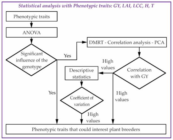
Figure 4.
Workflow diagram of the statistical analysis for phenotypic variation and relationship with yield.
From a plant breeding point of view, there are a variety of methods for studying genetic diversity, genetic proximity, and similarity [61,62]. Recently, multivariate methods have become increasingly popular [63,64]. To capture the phenotypic variation of the yield because of genetic diversity, we performed an analysis of variance (one-way ANOVA) on the retrieved biophysical variables and the agronomical traits according to [65]. After establishing the significant influence of the genotype factor on the variation of the studied traits, we proceeded to conduct Duncan’s multiple range test (DMRT) to measure specific differences between pairs of means.
Correlation analysis determines the strength and direction of the linear relationships between the studied traits. Principal component analysis (PCA) provides additional graphical information on the presence of correlations between the studied traits. PCA also provides information on the location of genotypes according to their values on individual traits for the main components.
The last step of our methodology is the analysis of the descriptive statistics of the phenotypic traits and particularly the coefficient of variation, which provides information on the genetic diversity. Lower values of the coefficient of variation are an indicator of low genetic diversity, and higher values are an indicator of significant genetic diversity.
3. Results
3.1. Biophysical Variables Retrieval
The best performing nonparametric method for all biophysical variables retrieval was GPR. The goodness-of-fit metrics for the optimised models and test dataset ranged for R2 from 0.20 to 0.62 and nRMSE from 18.43 to 24.02 (Table 8 and Figure 5). However, among the retrieved biophysical variables with GPR models, only LAI and LCC demonstrate average to high agreement with observations when validated to test dataset—R2 = 0.48, rRMSE = 13.51% and R2 = 0.62, rRMSE = 6.42%, respectively. Therefore, the subsequent analysis will be performed only with the modelled LAI and LCC with the GPR model. We will consider them as remotely sensed phenotypic traits, even if LAI and LCC tend to saturate for high values (Figure 5).
Table 8.
Results of biophysical variables retrieval with a nonparametric model, n_training = 260, n_test = 47. Levels of significance: ns. not significant; * p < 0.05; **p < 0.01. The best performing models for each variable are in bold.
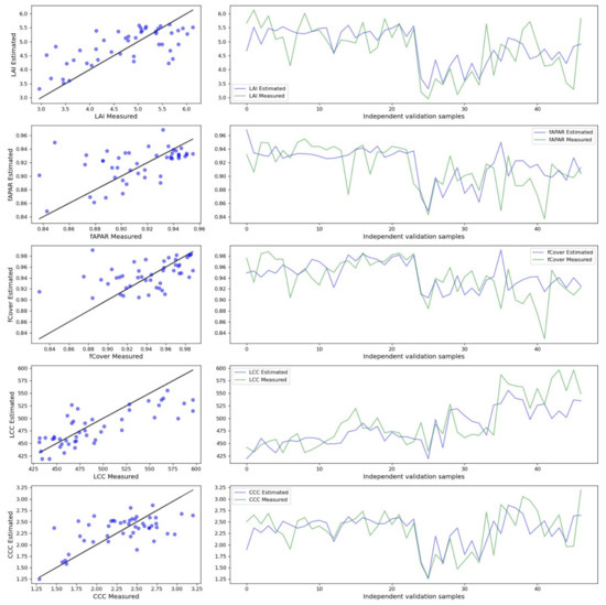
Figure 5.
Relationship between observed and predicted biophysical variables. The predicted biophysical variables are from the best performing nonparametric model (GPR). The black line is 1:1 line.
According to the cross-validation results, good models with parametric methods were found only for fAPAR and fCover with the goodness-of-fit metrics for the optimised models and test dataset, R2 from 0.35 to 0.49 and nRMSE from 0.65 to 0.69 (Table 9 and Figure 6). Both variables were best retrieved with 3BSI-Wang VI and polynomial function.
Table 9.
Results of biophysical variables retrieval with parametric models, n_training = 260, n_test = 47. Levels of significance: ns. not significant; * p < 0.05; ** p < 0.01. The best performing models for each variable are in bold.
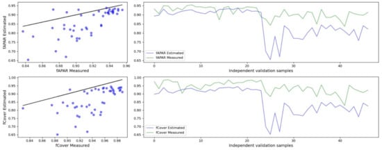
Figure 6.
Relationship between observed and predicted biophysical variables. The predicted biophysical variables are from the best performing parametric model (3BSI-Wang and polynomial function). The black line is 1:1 line.
3.2. GY Retrieval
We trained models with the two UAV campaigns data independently to compare which wheat phenological phase is better suited for GY retrieval. The best performing nonparametric method (Table 10) was again GPR and the parametric method (Table 11) was with 3-spectral-band index. Independently of the method used, the grain filling phenophase, or June campaign, was better suited for GY retrieval (Figure 7). The parametric model with 3BSI-Tian vegetation index and linear function had the better goodness-of-fit metrics for the optimised models and test dataset (Table 11 and Figure 7).
Table 10.
Results of GY retrieval with nonparametric models, n_training = 164, n_test = 55. Levels of significance: ns. not significant; * p < 0.05; ** p < 0.01. The best performing models for each variable are in bold.
Table 11.
Results of GY retrieval with parametric models, n_training = 164, n_test = 55. Levels of significance: ns. not significant; * p < 0.05; ** p < 0.01. The best performing models for each variable are in bold.
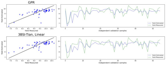
Figure 7.
Relationship between observed and predicted GY. The predicted GY is from the best performing nonparametric (GPR) and parametric (3BSI-Tian, linear) models in grain filling phenophase. The black line is 1:1 line.
3.3. Visual Inspection of the GY and Remotely Sensed Phenotypic Traits and Their Uncertainty Characterisation
The visual inspection of the retrieved LAI and LCC maps (Figure 8) shows that the LAI decreased from the flowering (LAI05) to the grain filling (LAI06) stage; however, LCC increased from flowering (LCC05) to grain filling (LCC06). Those results are in accordance with the in situ measurements (Table 2).
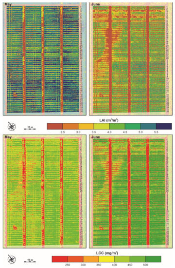
Figure 8.
UAV-obtained map of estimated LAI and LCC for both CVTs for flowering (May) and grain filling (June) phenological development stage. The LAI and LCC are estimated with the GPR model.
The uncertainty is characterised by the mean coefficient of variation (CV) generated by each GPR model. The mean and standard deviation of CV for LAI05 are much lower than those for LAI06: 16%, 1% and 28%, 12%, respectively. The mean and standard deviation of CV for LCC05 and LCC06 are almost constant: 8%, 0.5% and 10%, 2.6%, respectively.
Figure 9 shows the improved spatial resolution of the estimated pixel-level GY map compared with the map generated with the ground measurements. While traditionally only one value per plot for GY is measured, we have a high spatial resolution in the estimated GY that gives the breeder additional information for their analysis. It is visible in both maps (Figure 9A,B) that genotypes 1 to 6 from CVT1 are with a lower yield than the rest of the genotypes. The same could also be said for the III and IV replicates.
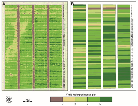
Figure 9.
(A) UAV-obtained map of the estimated GY. The GY was estimated with the parametric model 3BSI-Tian/linear from grain filling phenological development stage. (B) Vector map of GY measured by mechanical harvesting at full maturity of the plants.
3.4. Phenotypic Variation and Relationship with Yield
The analysis of variance (ANOVA) for both CVTs (Table A3) shows a significant difference between genotypes and significant differences in replicates. Significant differences between genotypes were found for the plant height (H) trait and no differences between replicates were observed. Therefore, genotypes have a major influence on the established variation of plant height. In CVT2, the differences between the genotypes were proven at a lower level for the traits: LAI06, LCC05, and LCC06. Genotypic differences are a prerequisite for an increased opportunity for effective selection.
With the highest yield is characterised genotype 23 in CVT1 (10.22 kg/plot) and genotype 14 in CVT2 (10.38 kg/plot), Table A4. For those two genotypes, the yield differs from the yield of all other genotypes because it falls into separate groups (h) and (j) according to the DMRT. The lowest statistically distinguishable yield of all other genotypes is genotype 3 in CVT1 (6.63 kg/plot) and 11 in CVT2 (8.32 kg/plot) which also fall into a separate group (a).
The correlation analysis (Figure 10) shows high positive correlations between yield (GY) and the following traits: LAI06, LCC05, and LCC06. GY has a negative correlation with H.
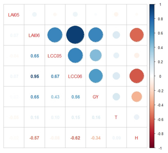
Figure 10.
Correlation analysis of studied traits: LAI05, LAI06, LCC05, LCC06, grain yield (GY), tillering (T), and plant height (H). Data from both CVTs are used. Only significant correlations (p < 0.05) are shown.
The performed PCA shows two main components, Factor 1 and Factor 2, which explains over 63% of the total variation in all genotype traits, which is high enough to correctly interpret the results (Figure 11). According to the angles between the vectors of the traits, the correlations between them can be judged. The more acute the angle, the stronger and more positive the correlation is. At right angles, the correlation is zero, and the obtuse angle indicates a negative correlation. The results from the PCA are in accordance with the correlation analysis and show that the yield has a strong positive correlation with LAI06, LCC05, LCC06 (Figure 11A).
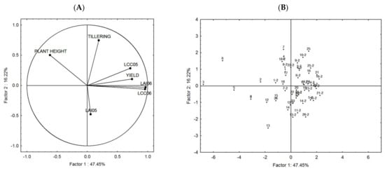
Figure 11.
PCA results with 7 traits, LAI05, LAI06, LCC05, LCC06, yield, tillering, and plant height, and both CVTs. The distribution between the traits (A) and the genotypes (B) within the two main components (Factor 1 and Factor 2) is visualised. The numbers in (B) are the genotypes’ codes, the ones without a suffix are from CVT1, and suffix-2 are from CVT2.
The distribution of genotype points in the Factor 1 to Factor 2 coordinate system is presented in Figure 11B. According to the quadrant in which the genotypes are located, we can judge the corresponding strongest influence of the specific trait. The genotypes positioned in the middle are balanced in terms of traits, while those placed in the periphery are influenced by a specific trait. Most of the genotypes are in the two right quadrants (Figure 11B), the same quadrants with the vectors of yield, LCC05, LCC06, and LAI06 (Figure 11A).
The results of the last step of our methodology for statistical analysis for phenotypic variation and relationship with yield, Figure 4, namely the coefficient of variation from the descriptive statistics of the phenotypic traits, are presented in Table 12.
Table 12.
Descriptive statistics of the studied phenotypic traits. LAI05, LAI06, LCC05, and LCC06 are modelled traits with GPR. GY, T, and H are ground-measured traits.
4. Discussion
4.1. Biophysical Variables and Yield Retrieval from UAV Data
When evaluating the performance of the retrieval models, some studies use cross-validation techniques [28,41,66], but fewer use test datasets [36,67]. Moreover, to train and evaluate a model with a certain confidence, a good amount of training/test samples is required. However, obtaining in situ field data is time consuming and expensive. Therefore, regression models are constructed with very different training/test sample numbers, from dozens [19,36,68] or hundreds [41,66]. In the present review, we use cross-validation to optimise the model and test dataset to evaluate its performance. The relatively large sample size (307 and 219 for biophysical variables and yield retrieval, respectively) in our study theoretically allows us to construct more robust models. In addition, note that for the biophysical variables modelling, the cross-validation results provide information about model performance across the almost full range of development stages. In contrast, the test results provide information about the model performance from the relatively late stages, flowering and grain filling.
All retrieval methods have their advantages and disadvantages [34]. We tested parametric and nonparametric regression models and our results show that the nonparametric models for biophysical variables retrieval are more robust (Table 8 and Table 9) than the parametric models. The greater flexibility of the nonparametric models is demonstrated in the retrieval of fAPAR and fCover (Figure 5 and Figure 6). In this case, it is also visible how the different goodness-of-fit metrics are complementary and that it is almost impossible to use only one or two of them. For example, the Pearson correlation coefficient is a measure of how closely the observations follow a straight line, but not necessarily the 1:1 line. The NSE coefficient is a measure of how well the observations follow the 1:1 line. Strong correlation expresses high precision, but not necessarily high accuracy [69]. The GPR method was clearly superior to the other four nonparametric regression methods tested in this study. According to the test results, it performed best for all estimated variables except GY in the flowering stage when better results show RFR.
The nonparametric GPR method was able to predict LAI with reasonable accuracy as shown by the cross-validation results (R2 = 0.81, RMSE = 0.84). The successful retrieval of LAI from Sequoia camera data was illustrated also by [70]. They used simple linear regression and MTVI2 index calculated from the Sequoia image bands to predict LAI (R2 = 0.61, RMSE = 1.17). Nevertheless, in our study the independent validation showed that the model did not perform particularly well for LAI values between 3 and 6. The less robust than expected performance of the LAI model in this range is probably due to the saturation of the spectral response for high LAI [41] (Figure 5). LCC retrieval is more robust than the LAI retrieval, even if LCC also presents saturation [71]. The LCC nonparametric modelling is an interesting case (Table 8) because even if the KRR is the best performing model with cross-validation, it is still the GPR that performed better with the test dataset.
The accuracy of LCC modelling in this study is comparable with previous studies. For example, a study from [72] estimated the LCC of wheat using hyperspectral UAV data. For the flowering stage, when the modelling was the most accurate, the best performing model (SVM) achieved an R2 value of 0.79 with a dataset of n = 32. In our study, the best performing model was GPR which achieved cross-validation results of R2 = 0.83 and test results of R2 = 0.62. Moreover, in our study, only four broad bands were used as predictors, whereas the study of [72] tested numerous narrow band spectral features.
In our study, we also tried to predict fAPAR, which is not so commonly used as a parameter in phenotyping experiments. A good result for fAPAR prediction with UAV RGB images and SVR (R2 of 0.86) was reported by [73]. This result is similar to our study, where the parametric model (3BSI-Wang/polynomial) achieved an R2 of 0.81 during the cross-validation. However, during the test, the parametric model achieved only R2 of 0.49. The problem of saturation is also present for fAPAR.
Previous studies indicated that the saturation issue of optical remote sensing can affect the performances of statistical regression models in estimating crop biophysical parameters [73,74]. To overcome the saturation problems inherent in the remotely sensed optical measurements, a multisource remote sensing fusion is proposed [30,73].
Another indicator of model robustness is the uncertainty estimation per pixel provided by the GPR models. The GPR model for LCC retrieval provided a slight increase in uncertainty from flowering (BBCH69-BBCH71) to grain filling (BBCH75-BBCH77) with a mean CV of 8% and 10%, respectively. For comparison, the mean CV of LAI is twice as high, with 16% and 28% for the two phenological stages, respectively. The standard deviation of CV between the two phases also increases for both biophysical variables, but while it is 5 times higher (from 0.5 to 2.6) for LCC, it is 12 times higher for LAI (from 1 to 12).
It is interesting to notice that when using parametric regression models, the biophysical variables are modelled by an exponential function [60,75]. However, in our case, it is a polynomial function that is better fitted to the training data. This difference comes from incorporating samples from bare soil in the training data.
We tested yield retrieval with parametric and nonparametric regression models with data from two phenological development stages, flowering (BBCH69-BBCH71) and grain filling (BBCH75-BBCH77), separately. In the general case, the models with grain filling data had better accuracy than those with flowering data. This pattern is observed for both the parametric and nonparametric models. Those results are in accordance with other studies [14]. They reported higher correlations with yield in rainfed trial with multispectral indices during the grain filling phase. Similar results were reported by [76] for a limited irrigation trail where yield was predicted most accurately using mid grain filling UAV-derived data. Other studies [19] report that yield prediction also improves with the advancement of the phase in the growing cycle, from the jointing stage to the flowering stage. They tested PLSR, artificial neural network (ANN), and RFR methods. Their best performing model was PLSR. In our study, PLSR also performed better than RFR but was outperformed by GPR.
Regarding the performance of different methods for GY retrieval, our results show that at the grain filling stage, the best parametric model (3BSI-Tian/linear) slightly outperforms the nonparametric (GPR), Table 10 and Table 11. At the flowering stage, the pattern is reversed, and a nonparametric method (in this case RFR) performed better than any parametric method. A previous comparison [67] of parametric and nonparametric models for GY retrieval has shown that the two types of methods, parametric and nonparametric, give similar results with minor superiority of parametric models. Even though the best performing method for yield differed between the two development stages, it cannot be argued that any method is more useful in one stage or the other. Moreover, in contrast with our study, [76] found that GPR performed best for flowering and RFR performed best for early grain filling when predicting wheat yield. As already discussed, GPR presents an advantage by providing uncertainty estimation for each retrieved pixel; therefore, giving invaluable spatial information on the uncertainty of the retrieved value. On the other hand, the parametric model is easily applicable and understandable with its linear function and three bands VI.
The accuracy of GY prediction in this study was lower (R2 = 0.49, rRMSE = 6.07% in grain filling) in comparison with some previous studies. For example, [77] achieved R2 = 0.93 using linear regression and a VI calculated from RGB-camera data. Using linear regression and data from the same camera as in this study, i.e., Sequoia, [17] modelled yield with maximal R2 of 0.89. Five-band UAV imagery was used by [78] in combination with least absolute shrinkage and selection operator (LASSO) and SVR to predict spring wheat yield. Both methods resulted in an R2 of 0.90. However, other studies reported moderate results, even though hyperspectral UAV data were used [19].
4.2. Remotely Sensed and Traditional Phenotypic Traits for Plant Breeding
We studied the possibilities of considering the biophysical variables retrieved from UAV multispectral data as phenotypic traits for plant breeders. To do so, first, we retrieved the biophysical variables, evaluated the models and, due to the performance of the models, chose LCC05, LCC06, LAI05, and LAI06. Then we applied a commonly used tool in breeding research, analysis of variance (ANOVA), to detect the statistically significant factors on which the variation of the studied traits depends and the differences between the tested genotypes. The ANOVA for both CVTs (Table A3) shows a significant difference between genotypes, both for the remotely sensed phenotypic traits LAI06, LCC05, LCC06 and for the traditional agronomic traits GY, H, T. Previous studies found similar results when considering yield and plant height [79,80] or other agronomic traits [81,82,83]. Remotely sensed spectral crop characteristics such as VIs have been previously shown to differ significantly between wheat genotypes [18,76]. We further show that the same is true for biophysical variables retrieved from such spectral characteristics. Because of the established significant difference between genotypes, we performed DMRT that gives us additional information on the differences in genotypes according to a certain phenotypic trait.
The PCA results and the correlation matrix can be used to illustrate the relationship between different traits. Our results show positive correlations between yield (GY) and the following traits: LCC05 (R2 = 0.43 at flowering stage), LAI06 and LCC06 (R2 = 0.46, 0.44 at grain filling stage). Similarly, [17] performed regression analysis between UAV-NDVI and GY for wheat in limited irrigated conditions but found that the coefficient of determination (R2 = 0.08) at early grain filling stages was much lower.
According to the results of the descriptive statistics presented in Table 12, high genetic diversity, in studied genotypes and among the considered remotely sensed phenotypic traits (LAI06, LCC05, LCC06), is found for LCC06 and LAI06. Therefore, they could be used in addition to the traditional phenotypic traits for plant breeding studies.
4.3. Limitations, Challenges, and Future Opportunities
While this study showed the application of parametric and nonparametric regression models for yield and phenotypic traits retrieval for plant breeding experiments, the approach poses some limitations and challenges. They are briefly listed below, followed by proposed solutions.
- (1)
- The developed biophysical variable retrieval models are overfitted and less robust than expected, except for LCC and LAI. The dataset was from two sites, one sown with winter durum wheat (Triticum turgidum L. var. durum), Chirpan, and the other winter wheat (Triticum aestivum L.), Zlatia. However, studies [36] suggest that the relationship between spectral data and biophysical variables is variety-specific. Hence, the robustness of the models throughout the season with data from the same site as well as from several consecutive harvest years remains to be evaluated.
- (2)
- Vegetation growth is a dynamic and accumulative process and representing it by just a few data acquisitions can be limiting. Differences found in certain phenophases can be compensated in others [84]. Including more dates and using multitemporal data would help to better describe crop growth [84,85]. Moreover, the selection of the phenological stage, and therefore UAV imagery dates, has an important impact on the capability to determine differences in the genotypes [84].
- (3)
- In the current study only four spectral broadbands are analysed, whereas spectroradiometers, or hyperspectral UAV imagery, provide many spectral narrow bands allowing for more accurate analysis and assessment of their correlation with a wider range of biophysical traits such as pigments other than chlorophyll, plant macronutrients, lignin and cellulose, polyphenols [86], or water content [87,88].
- (4)
- Uncertainty analysis was carried out only for uncertainties that arise from the parameterizations and assumptions specific to retrieval algorithms. This, however, is only one main category of uncertainty [89]. The uncertainty in the acquisition of in situ data by non-invasive methods can lead to important bias. Its correction can reduce the nRMSE between the non-invasive and destructive methods from 50% to 17% [90]. The last category is the errors referred to the sensor, including sensor calibrations and radiometric, geometric, and atmospheric corrections [34]. In addition, uncertainty propagation study is necessary to give the plant breeders a better understanding of the precision and accuracy of the proposed remote sensing phenotypic traits.
5. Conclusions
In our study we (1) retrieved biophysical variables from multispectral UAV data to complement the phenotypic traits that breeders traditionally collect; (2) proposed a retrieval method for rapid estimation of wheat grain yield through UAV platforms; (3) found significant differences between the genotypes in the two studied experiments (CVTs), and genotypes have a significant influence on the expression of traits. The application of PCA proves that most of the studied traits are related to yield and can be successfully used for preliminary yield assessment in wheat breeding.
Each breeding context is different, by the studied crop and breeders’ experience and aim. Nevertheless, UAV data reveal the variability present within each plot and between the different replicates and allow a much higher number of measurements compared to traditional breeders’ data collection. However, it is still under investigation as to which of the studied biophysical variables will play a role in plant breeding and variety testing. Monitoring the proposed phenotypic traits can be used for preliminary assessment of productivity.
We believe that those preliminary results could speed up crop improvement programs; however, stronger interdisciplinary research is still needed.
Author Contributions
Breeding design and experiment, V.B. and R.D.; conceptualisation, D.G., E.R. and V.B.; methodology, D.G., E.R. and V.B.; validation, D.G., E.R. and V.B.; formal analysis, D.G. and R.D.; investigation, D.G., E.R., R.D., A.G., G.J., P.D. and V.B.; resources, E.R. and V.B.; data curation, D.G., A.G., G.J., R.D., K.T. and P.D.; writing—original draft preparation, D.G.; writing—review and editing, E.R., P.D. and V.B.; visualisation, A.G. and G.J.; supervision, D.G. and E.R.; funding acquisition, E.R. and V.B. All authors have read and agreed to the published version of the manuscript.
Funding
This research was funded by the Bulgarian Ministry of Education and Science under the National Research Programme “Smart crop production” approved by the Decision of the Ministry Council №866/26.11.2020.
Institutional Review Board Statement
Not applicable.
Informed Consent Statement
Not applicable.
Data Availability Statement
Not applicable.
Acknowledgments
This publication is the result of the project implementation: “National Research Programme-Smart crop production” funded by the Bulgarian Ministry of Education and Science. Part of this publication data is from the project “Testing Sentinel-2 vegetation indices for the assessment of the state of winter crops in Bulgaria” (TS2AgroBg) project funded by the government of the Republic of Bulgaria through an ESA Contract (4000117474/16/NL/NDe) under the Plan for the European Cooperating States. Furthermore, this research was supported by the Action CA17134 SENSECO (Optical synergies for spatiotemporal sensing of scalable Ecophysiological traits) funded by COST (European Cooperation in Science and Technology, www.cost.eu, accessed on 30 December 2021).
Conflicts of Interest
The authors declare no conflict of interest.
Appendix A
Table A1.
Location of the varieties and breeding lines in CVTs and descriptive statistics for the ground-measured data for the GY (kg/plot) from each genotype. A plot is 13.2 m2 (12 × 1.10 m).
Table A1.
Location of the varieties and breeding lines in CVTs and descriptive statistics for the ground-measured data for the GY (kg/plot) from each genotype. A plot is 13.2 m2 (12 × 1.10 m).
| Competitive Variety Trial CVT 1 | Competitive Variety Trial CVT 2 | ||||||||||
|---|---|---|---|---|---|---|---|---|---|---|---|
| Genotype | Min. Value | Max. Value | Mean | Std. Dev | Genotype | Min. Value | Max. Value | Mean | Std. Dev | ||
| Code | Name | Code | Name | ||||||||
| 1 | Beloslava | 8.8 | 10.3 | 9.4 | 0.7 | 1 | D-8156 | 8.8 | 9.5 | 9.2 | 0.3 |
| 2 | Vazhod | 8.0 | 9.9 | 9.0 | 0.8 | 2 | D-8405 | 8.0 | 9.9 | 9.1 | 0.8 |
| 3 | Progres | 5.8 | 7.3 | 6.6 | 0.6 | 3 | D-8401 | 9.0 | 10.3 | 9.8 | 0.6 |
| 4 | Viktoriya | 8.0 | 10.3 | 9.2 | 0.9 | 4 | D-8298 | 8.0 | 9.4 | 9.0 | 0.7 |
| 5 | Zvezditsa | 7.9 | 9.3 | 8.5 | 0.6 | 5 | D-8379 | 9.8 | 10.0 | 10.0 | 0.1 |
| 6 | Deyana | 7.5 | 9.6 | 8.5 | 0.8 | 6 | D-8000 | 9.1 | 10.7 | 9.8 | 0.7 |
| 7 | Elbrus | 9.0 | 9.7 | 9.4 | 0.3 | 7 | D-8313 | 8.0 | 9.0 | 8.5 | 0.5 |
| 8 | Deni | 8.8 | 9.5 | 9.3 | 0.3 | 8 | DV-8417 | 9.0 | 9.9 | 9.3 | 0.4 |
| 9 | Trakiets | 9.0 | 10.5 | 9.6 | 0.7 | 9 | D-8404 | 8.4 | 10.0 | 9.3 | 0.7 |
| 10 | Kehlibar | 9.4 | 10.4 | 9.9 | 0.4 | 10 | D-8031 | 9.7 | 10.7 | 10.1 | 0.4 |
| 11 | Reyadur | 9.4 | 10.6 | 10.1 | 0.5 | 11 | D-8484 | 8.0 | 8.9 | 8.3 | 0.4 |
| 12 | Tserera | 8.8 | 9.7 | 9.2 | 0.4 | 12 | D-8456 | 9.0 | 9.5 | 9.2 | 0.2 |
| 13 | Mirela St | 7.8 | 9.1 | 8.4 | 0.7 | 13 | Mirela St | 8.9 | 9.0 | 8.9 | 0.1 |
| 14 | Predel St | 9.1 | 10.3 | 9.8 | 0.5 | 14 | Predel St | 10.2 | 10.7 | 10.4 | 0.2 |
| 15 | Raylidur | 8.9 | 10.0 | 9.7 | 0.5 | 15 | D-8471 | 9.8 | 10.1 | 10.0 | 0.1 |
| 16 | Saya | 9.1 | 10.6 | 10.1 | 0.7 | 16 | D-8472 | 9.7 | 10.2 | 9.8 | 0.2 |
| 17 | Heliks | 9.4 | 10.2 | 9.9 | 0.4 | 17 | D-8516 | 9.1 | 10.7 | 9.9 | 0.8 |
| 18 | Viomi | 9.3 | 9.9 | 9.6 | 0.3 | 18 | D-8346 | 8.6 | 10.6 | 9.8 | 0.9 |
| 19 | D-8159 | 9.8 | 10.1 | 9.9 | 0.1 | 19 | D-8469 | 9.2 | 10.8 | 10.0 | 0.6 |
| 20 | D-8243 | 9.8 | 10.2 | 10.0 | 0.2 | 20 | D-8495 | 10.1 | 10.4 | 10.3 | 0.2 |
| 21 | D-8327 | 9.8 | 10.9 | 10.2 | 0.5 | 21 | D-8483 | 9.9 | 10.6 | 10.1 | 0.3 |
| 22 | D-8091 | 9.1 | 9.5 | 9.3 | 0.2 | 22 | D-8299 | 9.1 | 9.3 | 9.2 | 0.1 |
| 23 | D-8148 | 9.9 | 10.6 | 10.2 | 0.3 | 23 | D-8551 | 9.1 | 10.3 | 9.8 | 0.5 |
| 24 | D-8326 | 8.4 | 9.8 | 9.3 | 0.6 | 24 | D-8271 | 9.1 | 10.1 | 9.6 | 0.4 |
| 25 | D-7553 | 9.3 | 10.2 | 9.8 | 0.4 | 25 | D-8527 | 9.7 | 10.3 | 10.0 | 0.2 |
| 26 | D-8036 | 8.0 | 10.0 | 9.1 | 0.9 | 26 | D-8526 | 8.7 | 9.1 | 9.0 | 0.18 |
Table A2.
Details of the ground-measured phenophases and plant height during the two field campaigns.
Table A2.
Details of the ground-measured phenophases and plant height during the two field campaigns.
| Field Campaign Competitive Variety Trial | Genotype Code in (Phenological Development Stage) | Genotype Code with (Plant Height in cm) |
|---|---|---|
| 27–28 May 2021 CVT 1 |
|
|
| 27–28 May 2021 CVT 2 |
|
|
| 16–17 June 2021 CVT 1 |
|
|
| 16–17 June 2021 CVT 2 |
|
|
Table A3.
ANOVA for CVT1 and CVT2. Tillering: T; plant height: H; sum of squares: SS; degree of freedom: DoF; mean squares: MS; F critical: F; significant: Sig; *—p ≤ 0.05; **—p ≤ 0.01; ***—p ≤ 0.001; n.s.—not significant.
Table A3.
ANOVA for CVT1 and CVT2. Tillering: T; plant height: H; sum of squares: SS; degree of freedom: DoF; mean squares: MS; F critical: F; significant: Sig; *—p ≤ 0.05; **—p ≤ 0.01; ***—p ≤ 0.001; n.s.—not significant.
| Trait | Source | SS CVT1 | DoF CVT1 | MS CVT1 | F CVT1 | Sig CVT1 | SS CVT2 | DoF CVT2 | MS CVT2 | F CVT2 | Sig CVT2 |
|---|---|---|---|---|---|---|---|---|---|---|---|
| LAI05 | Genotype | 5.053 | 25 | 0.202 | 26.6 | *** | 2.000 | 25 | 0.080 | 7.0 | *** |
| Replication | 0.294 | 3 | 0.098 | 12.9 | *** | 0.216 | 3 | 0.072 | 6.3 | *** | |
| Error | 0.570 | 75 | 0.008 | 0.853 | 75 | 0.011 | |||||
| LAI06 | Genotype | 19.433 | 25 | 0.777 | 19.82 | *** | 4.127 | 25 | 0.165 | 4.40 | ** |
| Replication | 3.041 | 3 | 1.014 | 25.84 | *** | 10.568 | 3 | 3.523 | 93.96 | *** | |
| Error | 2.942 | 75 | 0.039 | 2.812 | 75 | 0.037 | |||||
| LCC05 | Genotype | 10281 | 25 | 411 | 8.5 | *** | 3366 | 25 | 135 | 2.2 | * |
| Replication | 4067 | 3 | 1356 | 27.9 | *** | 12667 | 3 | 4222 | 69.2 | *** | |
| Error | 3647 | 75 | 49 | 4575 | 75 | 61 | |||||
| LCC06 | Genotype | 111898 | 25 | 4476 | 16.52 | *** | 33823 | 25 | 1353 | 4.77 | ** |
| Replication | 28780 | 3 | 9593 | 35.40 | *** | 46203 | 3 | 15401 | 54.33 | *** | |
| Error | 20325 | 75 | 271 | 21260 | 75 | 283 | |||||
| GY | Genotype | 57.319 | 25 | 2.293 | 8.36 | *** | 30.467 | 25 | 1.219 | 6.73 | *** |
| Replication | 4.038 | 3 | 1.346 | 4.91 | *** | 3.868 | 3 | 1.289 | 7.13 | *** | |
| Error | 20.573 | 75 | 0.274 | 13.572 | 75 | 0.181 | |||||
| T | Genotype | 25.826 | 25 | 1.033 | 13.45 | *** | 25.230 | 25 | 1.009 | 17.93 | *** |
| Replication | 1.936 | 3 | 0.645 | 8.40 | *** | 0.468 | 3 | 0.156 | 2.77 | * | |
| Error | 5.759 | 75 | 0.077 | 4.222 | 75 | 0.056 | |||||
| H | Genotype | 6010 | 25 | 240 | 836 | *** | 2522 | 25 | 101 | 294 | *** |
| Replication | 1 | 3 | 0 | 1 | n.s. | 2 | 3 | 1 | 2 | n.s. | |
| Error | 22 | 75 | 0 | 26 | 75 | 0 |
Table A4.
Mean values and DMRT for LAI05, LAI06, LCC05, LCC06, grain yield (GY), tillering (T), and plant height (H) for CVT1 and CVT2. Mean values (in each column) followed by the same letters have no proven differences at p < 0.05 according to DMRT. GC: genotype code.
Table A4.
Mean values and DMRT for LAI05, LAI06, LCC05, LCC06, grain yield (GY), tillering (T), and plant height (H) for CVT1 and CVT2. Mean values (in each column) followed by the same letters have no proven differences at p < 0.05 according to DMRT. GC: genotype code.
| GC | LAI05 | LAI06 | LCC05 | LCC06 | Yield | Tillering | H | |||||||
|---|---|---|---|---|---|---|---|---|---|---|---|---|---|---|
| CVT1 | ||||||||||||||
| 1 | 5.1 | fgh | 3.9 | gh | 433.6 | abcd | 474.5 | defghi | 9.37 | defgh | 4.5 | g | 102.5 | i |
| 2 | 4.9 | bc | 3.3 | c | 428.4 | ab | 455.1 | d | 9.03 | bcde | 3.7 | bcde | 104.7 | j |
| 3 | 5.1 | fg | 2.4 | a | 436.5 | abcd | 385.0 | a | 6.63 | a | 3.0 | a | 119.5 | n |
| 4 | 4.9 | bc | 3.8 | efgh | 459.5 | jkl | 465.2 | defg | 9.16 | bcdef | 3.7 | cde | 112.7 | m |
| 5 | 5.1 | defg | 2.9 | b | 431.5 | abc | 409.6 | bc | 8.51 | bcd | 3.1 | a | 112.2 | lm |
| 6 | 5.2 | ghij | 2.5 | a | 437.8 | abcde | 386.5 | ab | 8.47 | bc | 4.0 | ef | 120.5 | o |
| 7 | 5.1 | cdef | 3.7 | defg | 449.8 | fghijk | 471.1 | defghi | 9.42 | efgh | 4.5 | g | 111.5 | l |
| 8 | 5.3 | j | 2.9 | b | 436.0 | abcd | 419.2 | c | 9.27 | cdefg | 3.3 | abc | 104.5 | j |
| 9 | 5.2 | ghij | 3.8 | fgh | 448.0 | efghij | 497.5 | ijk | 9.57 | efgh | 3.2 | ab | 101.5 | h |
| 10 | 5.2 | fghi | 3.8 | efgh | 449.3 | fghijk | 494.4 | hijk | 9.87 | efgh | 3.2 | a | 101.5 | h |
| 11 | 5.1 | fgh | 3.9 | gh | 451.2 | fghijk | 489.3 | fghijk | 10.07 | gh | 3.7 | cde | 99.5 | e |
| 12 | 5.2 | fghi | 3.5 | cdef | 431.3 | abc | 453.5 | d | 9.16 | bcdef | 3.1 | a | 104.2 | j |
| 13 | 5.3 | ij | 3.5 | cde | 426.9 | a | 454.8 | d | 8.38 | b | 3.1 | a | 89.5 | a |
| 14 | 5.3 | ij | 3.7 | defg | 439.6 | bcdef | 469.1 | defgh | 9.78 | efgh | 3.2 | a | 96.5 | c |
| 15 | 5.0 | bcde | 3.4 | cd | 441.7 | cdefg | 457.8 | de | 9.67 | efgh | 2.9 | a | 100.5 | fg |
| 16 | 5.1 | efg | 3.9 | gh | 455.2 | ijkl | 492.3 | ghijk | 10.07 | gh | 4.2 | fg | 97.2 | cd |
| 17 | 5.0 | cdef | 3.7 | defg | 444.1 | defghi | 464.6 | defg | 9.93 | efgh | 3.7 | de | 104.5 | j |
| 18 | 5.1 | fgh | 3.7 | defg | 450.8 | fghijk | 467.7 | defgh | 9.54 | efgh | 3.2 | a | 109.2 | k |
| 19 | 5.0 | bcd | 3.9 | gh | 451.9 | ghijk | 498.0 | ijk | 9.89 | efgh | 3.3 | abc | 97.7 | d |
| 20 | 5.3 | j | 3.8 | efgh | 441.9 | cdefgh | 477.7 | defghi | 9.95 | fgh | 4.1 | efg | 95.5 | b |
| 21 | 4.4 | a | 4.1 | h | 460.5 | kl | 513.0 | k | 10.16 | gh | 3.1 | a | 95.5 | b |
| 22 | 5.0 | bcd | 3.9 | fgh | 450.2 | fghijk | 483.7 | efghij | 9.33 | cdefgh | 3.0 | a | 100.7 | gh |
| 23 | 5.4 | j | 3.7 | defg | 451.7 | ghijk | 466.4 | defg | 10.22 | h | 3.0 | a | 102.5 | i |
| 24 | 4.5 | a | 3.9 | gh | 453.5 | hijkl | 509.3 | jk | 9.29 | cdefg | 3.3 | abcd | 89.5 | a |
| 25 | 4.8 | b | 3.9 | gh | 463.2 | l | 489.5 | fghijk | 9.80 | efgh | 4.5 | g | 99.7 | ef |
| 26 | 5.3 | hij | 3.5 | cde | 449.0 | efghijk | 462.4 | def | 9.14 | bcdef | 3.0 | a | 105.0 | j |
| CVT2 | ||||||||||||||
| 1 | 5.3 | fghiklm | 3.5 | a | 448.6 | abc | 461.9 | ab | 9.17 | cde | 3.6 | bcd | 108.5 | n |
| 2 | 5.2 | efghi | 3.9 | bcdefghi | 449.6 | abcd | 500.5 | defghij | 9.12 | bcd | 4.6 | f | 101.5 | gh |
| 3 | 5.4 | ml | 4.2 | hi | 456.9 | bcdef | 507.2 | efghij | 9.83 | defghij | 4.0 | de | 99.5 | e |
| 4 | 5.0 | ab | 3.9 | bcdefghi | 455.0 | bcdef | 492.5 | cdefghi | 8.96 | abc | 4.2 | ef | 99 | de |
| 5 | 5.2 | efghik | 4.1 | efghi | 459.4 | bcdef | 500.7 | defghij | 9.95 | ghij | 3.0 | a | 99.5 | e |
| 6 | 5.1 | abcde | 3.9 | bcdefghi | 465.3 | f | 476.5 | abcd | 9.80 | defghij | 3.1 | a | 109.5 | o |
| 7 | 5.3 | efghikl | 3.7 | abcd | 454.5 | bcdef | 492.1 | cdefghi | 8.47 | ab | 3.4 | abc | 105.5 | l |
| 8 | 5.0 | abc | 3.7 | abcd | 465.1 | ef | 466.0 | abc | 9.33 | cdefgh | 3.3 | ab | 114.5 | p |
| 9 | 5.2 | bcdefg | 3.7 | abc | 454.6 | bcdef | 503.7 | defghij | 9.28 | cdefg | 4.5 | f | 104.5 | k |
| 10 | 5.2 | bcdef | 3.9 | bcdefg | 457.9 | bcdef | 488.0 | bcdefgh | 10.13 | ij | 4.4 | f | 107.5 | m |
| 11 | 5.4 | kml | 4.0 | cdefghi | 453.2 | abcdef | 513.9 | hij | 8.32 | a | 3.1 | a | 98.5 | d |
| 12 | 5.4 | l | 3.7 | abc | 454.0 | bcdef | 482.4 | abcdefg | 9.19 | cdef | 3.2 | a | 101.7 | hi |
| 13 | 5.3 | fghiklm | 3.7 | abcde | 447.2 | ab | 479.6 | abcdef | 8.93 | abc | 3.2 | a | 89.5 | a |
| 14 | 5.4 | ml | 3.9 | bcdefgh | 451.7 | abcde | 482.9 | abcdefg | 10.38 | j | 3.2 | a | 100.7 | fg |
| 15 | 5.4 | ikml | 4.1 | fghi | 455.6 | bcdef | 517.0 | ij | 9.95 | ghij | 3.3 | ab | 100.5 | f |
| 16 | 5.4 | ghiklm | 4.2 | ghi | 460.0 | bcdef | 518.6 | ij | 9.84 | efghij | 4.2 | ef | 99.5 | e |
| 17 | 5.2 | cdefg | 4.0 | defghi | 448.3 | ab | 501.2 | defghij | 9.89 | fghij | 3.7 | cd | 102.2 | hi |
| 18 | 5.1 | abcd | 3.5 | a | 440.8 | a | 459.9 | a | 9.79 | defghij | 4.5 | f | 103.2 | j |
| 19 | 5.4 | hikml | 4.2 | hi | 455.7 | bcdef | 518.3 | ij | 10.01 | hij | 3.8 | cd | 101.5 | gh |
| 20 | 5.4 | kml | 3.7 | abcde | 453.0 | abcdef | 479.2 | abcde | 10.29 | ij | 3.4 | abc | 102.5 | ij |
| 21 | 5.3 | fghiklm | 4.2 | i | 462.2 | def | 522.9 | j | 10.14 | ij | 3.2 | a | 102.5 | ij |
| 22 | 5.0 | a | 3.7 | ab | 462.1 | cdef | 476.3 | abcd | 9.15 | bcde | 3.8 | cd | 104.5 | k |
| 23 | 5.3 | fghiklm | 3.8 | abcdef | 459.0 | bcdef | 508.1 | fghij | 9.77 | defghij | 3.6 | bcd | 97.5 | c |
| 24 | 5.2 | bcdefg | 4.0 | bcdefghi | 462.3 | def | 510.6 | ghij | 9.63 | cdefghi | 3.6 | bcd | 99.5 | e |
| 25 | 5.2 | defgh | 4.0 | bcdefghi | 458.4 | bcdef | 505.9 | efghij | 10.03 | hij | 4.2 | ef | 103.2 | j |
| 26 | 5.4 | ml | 4.0 | cdefghi | 453.8 | bcdef | 507.9 | fghij | 8.97 | abc | 3.2 | a | 92.5 | b |
References
- Dragov, R.; Dechev, D. Phenotypic Stability of Yield on Varieties and Lines of Durum Wheat (Triticum durum Desf.). Agric. Sci. Technol. 2015, 7, 204–207. [Google Scholar]
- Dimitrov, E.; Uhr, Z.; Velcheva, N. Genetic Distance of Common Winter Wheat Varieties. Genetika 2021, 53, 521–532. [Google Scholar] [CrossRef]
- Chawade, A.; Van Ham, J.; Blomquist, H.; Bagge, O.; Alexandersson, E.; Ortiz, R. High-Throughput Field-Phenotyping Tools for Plant Breeding and Precision Agriculture. Agronomy 2019, 9, 258. [Google Scholar] [CrossRef] [Green Version]
- Sankaran, S.; Khot, L.R.; Espinoza, C.Z.; Jarolmasjed, S.; Sathuvalli, V.R.; Vandemark, G.J.; Miklas, P.N.; Carter, A.H.; Pumphrey, M.O.; Knowles, N.R.; et al. Low-Altitude, High-Resolution Aerial Imaging Systems for Row and Field Crop Phenotyping: A Review. Eur. J. Agron. 2015, 70, 112–123. [Google Scholar] [CrossRef]
- Araus, J.L.; Cairns, J.E. Field High-Throughput Phenotyping: The New Crop Breeding Frontier. Trends Plant Sci. 2014, 19, 52–61. [Google Scholar] [CrossRef]
- Jin, X.; Zarco-Tejada, P.J.; Schmidhalter, U.; Reynolds, M.P.; Hawkesford, M.J.; Varshney, R.K.; Yang, T.; Nie, C.; Li, Z.; Ming, B.; et al. High-Throughput Estimation of Crop Traits: A Review of Ground and Aerial Phenotyping Platforms. IEEE Geosci. Remote Sens. Mag. 2021, 9, 200–231. [Google Scholar] [CrossRef]
- Atkinson, J.A.; Jackson, R.J.; Bentley, A.R.; Ober, E.; Wells, D.M. Field Phenotyping for the Future. Annu. Plant Rev. Online 2018, 1, 719–736. [Google Scholar] [CrossRef] [Green Version]
- Xie, C.; Yang, C. A Review on Plant High-Throughput Phenotyping Traits Using UAV-Based Sensors. Comput. Electron. Agric. 2020, 178, 105731. [Google Scholar] [CrossRef]
- Qiu, R.; Wei, S.; Zhang, M.; Li, H.; Sun, H.; Liu, G.; Li, M. Sensors for Measuring Plant Phenotyping: A Review. Int. J. Agric. Biol. Eng. 2018, 11, 1–17. [Google Scholar] [CrossRef] [Green Version]
- Feng, L.; Chen, S.; Zhang, C.; Zhang, Y.; He, Y. A Comprehensive Review on Recent Applications of Unmanned Aerial Vehicle Remote Sensing with Various Sensors for High-Throughput Plant Phenotyping. Comput. Electron. Agric. 2021, 182, 106033. [Google Scholar] [CrossRef]
- Machwitz, M.; Pieruschka, R.; Berger, K.; Schlerf, M.; Aasen, H.; Fahrner, S.; Jiménez-Berni, J.; Baret, F.; Rascher, U. Bridging the Gap Between Remote Sensing and Plant Phenotyping—Challenges and Opportunities for the Next Generation of Sustainable Agriculture. Front. Plant Sci. 2021, 12, 749374. [Google Scholar] [CrossRef]
- Shi, Y.; Thomasson, J.A.; Murray, S.C.; Pugh, N.A.; Rooney, W.L.; Shafian, S.; Rajan, N.; Rouze, G.; Morgan, C.L.; Neely, H.L.; et al. Unmanned Aerial Vehicles for High-Throughput Phenotyping and Agronomic Research. PLoS ONE 2016, 11, e0159781. [Google Scholar] [CrossRef] [Green Version]
- Bhandari, M.; Ibrahim, A.M.H.; Xue, Q.; Jung, J.; Chang, A.; Rudd, J.C.; Maeda, M.; Rajan, N.; Neely, H.; Landivar, J. Assessing Winter Wheat Foliage Disease Severity Using Aerial Imagery Acquired from Small Unmanned Aerial Vehicle (UAV). Comput. Electron. Agric. 2020, 176, 105665. [Google Scholar] [CrossRef]
- Gracia-Romero, A.; Kefauver, S.C.; Fernandez-Gallego, J.A.; Vergara-Díaz, O.; Nieto-Taladriz, M.T.; Araus, J.L. UAV and Ground Image-Based Phenotyping: A Proof of Concept with Durum Wheat. Remote Sens. 2019, 11, 1244. [Google Scholar] [CrossRef] [Green Version]
- Holman, F.H.; Riche, A.B.; Michalski, A.; Castle, M.; Wooster, M.J.; Hawkesford, M.J. High Throughput Field Phenotyping of Wheat Plant Height and Growth Rate in Field Plot Trials Using UAV Based Remote Sensing. Remote Sens. 2016, 8, 1031. [Google Scholar] [CrossRef]
- Hassan, M.A.; Yang, M.; Rasheed, A.; Jin, X.; Xia, X.; Xiao, Y.; He, Z. Time-Series Multispectral Indices from Unmanned Aerial Vehicle Imagery Reveal Senescence Rate in Bread Wheat. Remote Sens. 2018, 10, 809. [Google Scholar] [CrossRef] [Green Version]
- Hassan, M.A.; Yang, M.; Rasheed, A.; Yang, G.; Reynolds, M.; Xia, X.; Xiao, Y.; He, Z. A Rapid Monitoring of NDVI across the Wheat Growth Cycle for Grain Yield Prediction Using a Multi-Spectral UAV Platform. Plant Sci. 2019, 282, 95–103. [Google Scholar] [CrossRef]
- Kyratzis, A.C.; Skarlatos, D.P.; Menexes, G.C.; Vamvakousis, V.F.; Katsiotis, A. Assessment of Vegetation Indices Derived by UAV Imagery for Durum Wheat Phenotyping under a Water Limited and Heat Stressed Mediterranean Environment. Front. Plant Sci. 2017, 8, 1114. [Google Scholar] [CrossRef] [Green Version]
- Tao, H.; Feng, H.; Xu, L.; Miao, M.; Yang, G.; Yang, X.; Fan, L. Estimation of the Yield and Plant Height of Winter Wheat Using UAV-Based Hyperspectral Images. Sensors 2020, 20, 1231. [Google Scholar] [CrossRef] [Green Version]
- Buchaillot, M.; Gracia-Romero, A.; Vergara-Diaz, O.; Zaman-Allah, M.A.; Tarekegne, A.; Cairns, J.E.; Prasanna, B.M.; Araus, J.L.; Kefauver, S.C. Evaluating Maize Genotype Performance under Low Nitrogen Conditions Using RGB UAV Phenotyping Techniques. Sensors 2019, 19, 1815. [Google Scholar] [CrossRef] [Green Version]
- Castro, W.; Marcato, J., Jr.; Polidoro, C.; Osco, L.P.; Gonçalves, W.; Rodrigues, L.; Santos, M.; Jank, L.; Barrios, S.; Valle, C.; et al. Deep Learning Applied to Phenotyping of Biomass in Forages with UAV-Based RGB Imagery. Sensors 2020, 20, 4802. [Google Scholar] [CrossRef] [PubMed]
- Han, L.; Yang, G.; Yang, H.; Xu, B.; Li, Z.; Yang, X. Clustering Field-Based Maize Phenotyping of Plant-Height Growth and Canopy Spectral Dynamics Using a UAV Remote-Sensing Approach. Front. Plant Sci. 2018, 9, 1638. [Google Scholar] [CrossRef] [PubMed] [Green Version]
- Su, W.; Zhang, M.; Bian, D.; Liu, Z.; Huang, J.; Wang, W.; Wu, J.; Guo, H. Phenotyping of Corn Plants Using Unmanned Aerial Vehicle (UAV) Images. Remote Sens. 2019, 11, 2021. [Google Scholar] [CrossRef] [Green Version]
- Chivasa, W.; Mutanga, O.; Biradar, C. UAV-Based Multispectral Phenotyping for Disease Resistance to Accelerate Crop Improvement under Changing Climate Conditions. Remote Sens. 2020, 12, 2445. [Google Scholar] [CrossRef]
- Stewart, E.L.; Wiesner-Hanks, T.; Kaczmar, N.; DeChant, C.; Wu, H.; Lipson, H.; Nelson, R.J.; Gore, M.A. Quantitative Phenotyping of Northern Leaf Blight in UAV Images Using Deep Learning. Remote Sens. 2019, 11, 2209. [Google Scholar] [CrossRef] [Green Version]
- Di Gennaro, S.F.; Rizza, F.; Badeck, F.W.; Berton, A.; Delbono, S.; Gioli, B.; Toscano, P.; Zaldei, A.; Matese, A. UAV-Based High-Throughput Phenotyping to Discriminate Barley Vigour with Visible and near-Infrared Vegetation Indices. Int. J. Remote Sens. 2018, 39, 5330–5344. [Google Scholar] [CrossRef]
- Kefauver, S.C.; Vicente, R.; Vergara-Díaz, O.; Fernandez-Gallego, J.A.; Kerfal, S.; Lopez, A.; Melichar, J.P.; Serret Molins, M.D.; Araus, J.L. Comparative UAV and Field Phenotyping to Assess Yield and Nitrogen Use Efficiency in Hybrid and Conventional Barley. Front. Plant Sci. 2017, 8, 1733. [Google Scholar] [CrossRef]
- Jay, S.; Maupas, F.; Bendoula, R.; Gorretta, N. Retrieving LAI, Chlorophyll and Nitrogen Contents in Sugar Beet Crops from Multi-Angular Optical Remote Sensing: Comparison of Vegetation Indices and PROSAIL Inversion for Field Phenotyping. Field Crops Res. 2017, 210, 33–46. [Google Scholar] [CrossRef] [Green Version]
- Lyu, S.; Noguchi, N.; Ospina, R.; Kishima, Y. Development of Phenotyping System Using Low Altitude UAV Imagery and Deep Learning. Int. J. Agric. Biol. Eng. 2021, 14, 207–215. [Google Scholar] [CrossRef]
- Maimaitijiang, M.; Sagan, V.; Sidike, P.; Hartling, S.; Esposito, F.; Fritschi, F.B. Soybean Yield Prediction from UAV Using Multimodal Data Fusion and Deep Learning. Remote Sens. Environ. 2020, 237, 111599. [Google Scholar] [CrossRef]
- Pantazi, X.E.; Moshou, D.; Alexandridis, T.; Whetton, R.L.; Mouazen, A.M. Wheat Yield Prediction Using Machine Learning and Advanced Sensing Techniques. Comput. Electron. Agric. 2016, 121, 57–65. [Google Scholar] [CrossRef]
- Yoosefzadeh-Najafabadi, M.; Tulpan, D.; Eskandari, M. Using Hybrid Artificial Intelligence and Evolutionary Optimization Algorithms for Estimating Soybean Yield and Fresh Biomass Using Hyperspectral Vegetation Indices. Remote Sens. 2021, 13, 2555. [Google Scholar] [CrossRef]
- GEOGLAM Essential Agricultural Variables Working Group. Available online: https://earthobservations.org/geoglam.php?t=eo_data_coordination&s1=eodc_eav_wg (accessed on 3 November 2021).
- Verrelst, J.; Malenovský, Z.; Van der Tol, C.; Camps-Valls, G.; Gastellu-Etchegorry, J.-P.; Lewis, P.; North, P.; Moreno, J. Quantifying Vegetation Biophysical Variables from Imaging Spectroscopy Data: A Review on Retrieval Methods. Surv. Geophys. 2019, 40, 589–629. [Google Scholar] [CrossRef] [Green Version]
- Serrano, L.; Filella, I.; Peñuelas, J. Remote Sensing of Biomass and Yield of Winter Wheat under Different Nitrogen Supplies. Crop Sci. 2000, 40, 723–731. [Google Scholar] [CrossRef] [Green Version]
- Dimitrov, P.; Kamenova, I.; Roumenina, E.; Filchev, L.; Ilieva, I.; Jelev, G.; Gikov, A.; Banov, M.; Krasteva, V.; Kolchakov, V.; et al. Estimation of Biophysical and Biochemical Variables of Winter Wheat through Sentinel-2 Vegetation Indices. Bulg. J. Agric. Sci. 2019, 25, 14. [Google Scholar]
- Rivera, J.P.; Verrelst, J.; Delegido, J.; Veroustraete, F.; Moreno, J. On the Semi-Automatic Retrieval of Biophysical Parameters Based on Spectral Index Optimization. Remote Sens. 2014, 6, 4927–4951. [Google Scholar] [CrossRef] [Green Version]
- Berger, K.; Verrelst, J.; Féret, J.-B.; Wang, Z.; Wocher, M.; Strathmann, M.; Danner, M.; Mauser, W.; Hank, T. Crop Nitrogen Monitoring: Recent Progress and Principal Developments in the Context of Imaging Spectroscopy Missions. Remote Sens. Environ. 2020, 242, 111758. [Google Scholar] [CrossRef]
- Chlingaryan, A.; Sukkarieh, S.; Whelan, B. Machine Learning Approaches for Crop Yield Prediction and Nitrogen Status Estimation in Precision Agriculture: A Review. Comput. Electron. Agric. 2018, 151, 61–69. [Google Scholar] [CrossRef]
- Yang, G.; Liu, J.; Zhao, C.; Li, Z.; Huang, Y.; Yu, H.; Xu, B.; Yang, X.; Zhu, D.; Zhang, X.; et al. Unmanned Aerial Vehicle Remote Sensing for Field-Based Crop Phenotyping: Current Status and Perspectives. Front. Plant Sci. 2017, 8, 1111. [Google Scholar] [CrossRef]
- Verrelst, J.; Pablo, J.; Veroustraete, F.; Muñoz-Marí, J.; Clevers, J.G.P.W.; Camps-valls, G.; Moreno, J. Experimental Sentinel-2 LAI Estimation Using Parametric, Non-Parametric and Physical Retrieval Methods—A Comparison. ISPRS J. Photogramm. Remote Sens. 2015, 108, 260–272. [Google Scholar] [CrossRef]
- IUSS Working Group WRB. World Reference Base for Soil Resources 2014. International Soil Classification System for Naming Soils and Creating Legends for Soil Maps. Update 2015; FAO, Ed.; Food and Agriculture Organization of the United Nations: Rome, Italy, 2015. [Google Scholar]
- Panayotova, G.; Kostadinova, S.; Aleksieva, S.; Slavova, N.; Aladzhova, C.; Kostadinova, S.; Aleksieva, S.; Slavova, N.; Aladzhova, C. Nitrogen and phosphorus balances as dependent on durum wheat fertilization. Bulg. J. Agric. Sci. 2018, 24, 9–17. [Google Scholar]
- Meier, U. Growth Stages of Mono and Dicotyledonous Plants. BBCH Monograph, 2nd ed.; Federal Biological Research Centre for Agriculture and Forestry: Bonn, Germany, 2001. [Google Scholar]
- Meier, U. (Ed.) Growth Stages of Mono- and Dicotyledonous Plants. BBCH Monograph; Julius Kühn-Institut: Quedlinburg, Germany, 2018. [Google Scholar]
- Ganeva, D.; Roumenina, E.; Jelev, G.; Banov, M.; Krasteva, V.; Kolchakov, V. Applicability of Parametric and Nonparametric Regression Models for Retrieval of Crop Canopy Parameters for Winter Rapeseed and Wheat Crops Using Sentinel-2 Multispectral Data. In Proceedings of the Seventh International Conference on Remote Sensing and Geoinformation of the Environment (RSCy2019), Paphos, Cyprus, 27 June 2019; Volume 11174. [Google Scholar]
- Roumenina, E.; Jelev, G.; Dimitrov, P.; Filchev, L.; Kamenova, I.; Gikov, A.; Banov, M.; Veneta, K. Qualitative Evaluation and Within-Field Mapping of Winter Wheat Crop Condition Using Multispectral Remote Sensing Data. Bulg. J. Agric. Sci. 2020, 26, 1129–1142. [Google Scholar]
- Geladi, P.; Kowalski, B.R. Partial Least-Squares Regression: A Tutorial. Anal. Chim. Acta 1986, 185, 1–17. [Google Scholar] [CrossRef]
- Breiman, L. Random Forests. Mach. Learn. 2001, 45, 5–32. [Google Scholar] [CrossRef] [Green Version]
- Vapnik, V.; Golowich, S.; Smola, A. Support Vector Method for Function Approximation, Regression Estimation and Signal Processing. In Proceedings of the 9th International Conference on Neural Information Processing Systems, Denver, CO, USA, 3–5 December 1996; Volume 9, pp. 281–287. [Google Scholar]
- Suykens, J.A.K.; Vandewalle, J. Least Squares Support Vector Machine Classifiers. Neural Process. Lett. 1999, 9, 293–300. [Google Scholar] [CrossRef]
- Rasmussen, C.; Williams, C. Gaussian Processes for Machine Learning; The MIT Press: New York, NY, USA, 2006. [Google Scholar]
- Ganeva, D. Semiautomatic Retrieval of Biomass Based on Vegetation Index Optimization and Learning Machine Methods for Winter Rapeseed Crops. In Proceedings of the SES 2018—Fourteenth International Scientific Conference—Space, Ecology, Safety, Sofia, Bulgaria, 7–9 November 2018; pp. 299–305. [Google Scholar]
- Richter, K.; Atzberger, C.; Hank, T.B.; Mauser, W. Derivation of Biophysical Variables from Earth Observation Data: Validation and Statistical Measures. J. Appl. Remote Sens. 2012, 6, 1–24. [Google Scholar] [CrossRef]
- Le Maire, G.; François, C.; Dufrêne, E. Towards Universal Broad Leaf Chlorophyll Indices Using PROSPECT Simulated Database and Hyperspectral Reflectance Measurements. Remote Sens. Environ. 2004, 89, 1–28. [Google Scholar] [CrossRef]
- Clevers, J.G.P.W.; Gitelson, A.A. Remote Estimation of Crop and Grass Chlorophyll and Nitrogen Content Using Red-Edge Bands on Sentinel-2 and -3. Int. J. Appl. Earth Obs. Geoinf. 2013, 23, 344–351. [Google Scholar] [CrossRef]
- Tian, Y.C.; Gu, K.J.; Chu, X.; Yao, X.; Cao, W.X.; Zhu, Y. Comparison of Different Hyperspectral Vegetation Indices for Canopy Leaf Nitrogen Concentration Estimation in Rice. Plant Soil 2013, 376, 193–209. [Google Scholar] [CrossRef]
- Wang, W.; Yao, X.; Yao, X.; Tian, Y.; Liu, X.; Ni, J.; Cao, W.; Zhu, Y. Estimating Leaf Nitrogen Concentration with Three-Band Vegetation Indices in Rice and Wheat. Field Crops Res. 2012, 129, 90–98. [Google Scholar] [CrossRef]
- Dash, J.; Curran, P.J. Evaluation of the MERIS Terrestrial Chlorophyll Index (MTCI). Adv. Space Res. 2007, 39, 100–104. [Google Scholar] [CrossRef]
- Verrelst, J.; Rivera, J.P.; Moreno, J.; Camps-Valls, G. Gaussian Processes Uncertainty Estimates in Experimental Sentinel-2 LAI and Leaf Chlorophyll Content Retrieval. ISPRS J. Photogramm. Remote Sens. 2013, 86, 157–167. [Google Scholar] [CrossRef]
- Islam, M.R.; Faruquei, M.A.B.; Bhuiyan, M.A.R.; Biswas, P.S.; Salam, M.A. Genetic Diversity in Irrigated Rice. Pak. J. Biol. Sci. 2004, 7, 226–229. [Google Scholar] [CrossRef]
- Khodadadi, M.; Fotokian, M.H.; Miransari, M. Genetic Diversity of Wheat (Triticum aestivum L.) Genotypes Based on Cluster and Principal Component Analyses for Breeding Strategies. Aust. J. Crop Sci. 2011, 5, 17–24. [Google Scholar]
- Kabir, R.; Intikhab, A.; Zahoor, M.; Ahmed, I.; Khan, B.; Zakriya, M.; Rehman, M.; Muneer, M.; Munir, M. Multivariate Analysis of Genetic Divergence in Wheat (Triticuma estivum) Using Yield Traits. Int. J. Biosci. IJB 2017, 11, 43–48. [Google Scholar] [CrossRef]
- Dragov, R.; Dechev, D.; Taneva, K. Genetic Distance of New Bulgarian Durum Wheat Varieties and Breeding Lines of FCI-Chirpan, Bulgaria. Int. J. Innov. Approaches Agric. Res. 2019, 3, 402–410. [Google Scholar] [CrossRef]
- Lidanski, T. Statistical Methods in Biology and Agriculture; Zemizdat: Sofia, Bulgaria, 1988. [Google Scholar]
- Yue, J.; Feng, H.; Yang, G.; Li, Z. A Comparison of Regression Techniques for Estimation of Above-Ground Winter Wheat Biomass Using Near-Surface Spectroscopy. Remote Sens. 2018, 10, 66. [Google Scholar] [CrossRef] [Green Version]
- Zhou, X.; Kono, Y.; Win, A.; Matsui, T.; Tanaka, T.S.T. Predicting Within-Field Variability in Grain Yield and Protein Content of Winter Wheat Using UAV-Based Multispectral Imagery and Machine Learning Approaches. Plant Prod. Sci. 2021, 24, 137–151. [Google Scholar] [CrossRef]
- Ganeva, D.; Roumenina, E. Remote Estimation of Crop Canopy Parameters by Statistical Regression Algorithms for Winter Rapeseed Using Sentinel-2 Multispectral Images. Aerosp. Res. Bulg. 2018, 30, 75–95. [Google Scholar] [CrossRef]
- Svensgaard, J.; Jensen, S.M.; Christensen, S.; Rasmussen, J. The Importance of Spectral Correction of UAV-Based Phenotyping with RGB Cameras. Field Crops Res. 2021, 269, 108177. [Google Scholar] [CrossRef]
- Rufo, R.; Soriano, J.M.; Villegas, D.; Royo, C.; Bellvert, J. Using Unmanned Aerial Vehicle and Ground-Based RGB Indices to Assess Agronomic Performance of Wheat Landraces and Cultivars in a Mediterranean-Type Environment. Remote Sens. 2021, 13, 1187. [Google Scholar] [CrossRef]
- Berger, K.; Atzberger, C.; Danner, M.; Wocher, M.; Mauser, W.; Hank, T. Model-Based Optimization of Spectral Sampling for the Retrieval of Crop Variables with the PROSAIL Model. Remote Sens. 2018, 10, 2063. [Google Scholar] [CrossRef] [Green Version]
- Zhu, W.; Sun, Z.; Yang, T.; Li, J.; Peng, J.; Zhu, K.; Li, S.; Gong, H.; Lyu, Y.; Li, B.; et al. Estimating Leaf Chlorophyll Content of Crops via Optimal Unmanned Aerial Vehicle Hyperspectral Data at Multi-Scales. Comput. Electron. Agric. 2020, 178, 105786. [Google Scholar] [CrossRef]
- Lv, Z.; Meng, R.; Man, J.; Zeng, L.; Wang, M.; Xu, B.; Gao, R.; Sun, R.; Zhao, F. Modeling of Winter Wheat FAPAR by Integrating Unmanned Aircraft Vehicle-Based Optical, Structural and Thermal Measurement. Int. J. Appl. Earth Obs. Geoinf. 2021, 102, 102407. [Google Scholar] [CrossRef]
- Cai, W.; Zhao, S.; Wang, Y.; Peng, F.; Heo, J.; Duan, Z. Estimation of Winter Wheat Residue Coverage Using Optical and SAR Remote Sensing Images. Remote Sens. 2019, 11, 1163. [Google Scholar] [CrossRef] [Green Version]
- Lelong, C.C.D.; Burger, P.; Jubelin, G.; Roux, B.; Labbé, S.; Baret, F. Assessment of Unmanned Aerial Vehicles Imagery for Quantitative Monitoring of Wheat Crop in Small Plots. Sensors 2008, 8, 3557–3585. [Google Scholar] [CrossRef]
- Fei, S.; Hassan, M.A.; He, Z.; Chen, Z.; Shu, M.; Wang, J.; Li, C.; Xiao, Y. Assessment of Ensemble Learning to Predict Wheat Grain Yield Based on UAV-Multispectral Reflectance. Remote Sens. 2021, 13, 2338. [Google Scholar] [CrossRef]
- Zeng, L.; Peng, G.; Meng, R.; Man, J.; Li, W.; Xu, B.; Lv, Z.; Sun, R. Wheat Yield Prediction Based on Unmanned Aerial Vehicles-Collected Red–Green–Blue Imagery. Remote Sens. 2021, 13, 2937. [Google Scholar] [CrossRef]
- Shafiee, S.; Lied, L.M.; Burud, I.; Dieseth, J.A.; Alsheikh, M.; Lillemo, M. Sequential Forward Selection and Support Vector Regression in Comparison to LASSO Regression for Spring Wheat Yield Prediction Based on UAV Imagery. Comput. Electron. Agric. 2021, 183, 106036. [Google Scholar] [CrossRef]
- Abinasa, M.; Ayana, A.; Bultosa, G. Genetic Variability, Heritability and Trait Associations in Durum Wheat (Triticum turgidum L. Var. Durum) Genotypes. Afr. J. Agric. Res. 2011, 6, 3972–3979. [Google Scholar]
- Tesfaye, T.; Genet, T.; Desalegn, T. Genetic Variability, Heritability and Genetic Diversity of Bread Wheat (Triticum aestivum L.) Genotype in Western Amhara Region, Ethiopia. Wudpecker J. Agric. Res. 2014, 3, 26–34. [Google Scholar]
- Desheva, G.; Cholakov, T. Variability, Heritability and Genetic Progress for Some Yield Components in Common Winter Wheat Genotypes (Triticum aestivum L.). Genet. Plant Physiol. 2014, 4, 191–200. [Google Scholar]
- Mohammadi, R.; Farshadfar, E.; Amri, A. Interpreting Genotype×environment Interactions for Grain Yield of Rainfed Durum Wheat in Iran. Crop J. 2015, 3, 526–535. [Google Scholar] [CrossRef] [Green Version]
- Kaya, Y.; Turkoz, M. Evaluation of genotype by environment interaction for grain yield in durum wheat using non-parametric stability statistics. Turk. J. Field Crops 2016, 21, 50. [Google Scholar] [CrossRef]
- Campos, I.; González-Gómez, L.; Villodre, J.; Calera, M.; Campoy, J.; Jiménez, N.; Plaza, C.; Sánchez-Prieto, S.; Calera, A. Mapping Within-Field Variability in Wheat Yield and Biomass Using Remote Sensing Vegetation Indices. Precis. Agric. 2019, 20, 214–236. [Google Scholar] [CrossRef]
- Borra-Serrano, I.; De Swaef, T.; Quataert, P.; Aper, J.; Saleem, A.; Saeys, W.; Somers, B.; Roldán-Ruiz, I.; Lootens, P. Closing the Phenotyping Gap: High Resolution UAV Time Series for Soybean Growth Analysis Provides Objective Data from Field Trials. Remote Sens. 2020, 12, 1644. [Google Scholar] [CrossRef]
- Homolová, L.; Malenovský, Z.; Clevers, J.G.P.W.; García-Santos, G.; Schaepman, M.E. Review of Optical-Based Remote Sensing for Plant Trait Mapping. Ecol. Complex. 2013, 15, 1–16. [Google Scholar] [CrossRef] [Green Version]
- Pasqualotto, N.; Delegido, J.; Van Wittenberghe, S.; Verrelst, J.; Rivera, J.P.; Moreno, J. Retrieval of Canopy Water Content of Different Crop Types with Two New Hyperspectral Indices: Water Absorption Area Index and Depth Water Index. Int. J. Appl. Earth Obs. Geoinf. 2018, 67, 69–78. [Google Scholar] [CrossRef]
- Chen, S.; Chen, Y.; Chen, J.; Zhang, Z.; Fu, Q.; Bian, J.; Cui, T.; Ma, Y. Retrieval of Cotton Plant Water Content by UAV-Based Vegetation Supply Water Index (VSWI). Int. J. Remote Sens. 2020, 41, 4389–4407. [Google Scholar] [CrossRef]
- Malenovský, Z.; Homolová, L.; Lukeš, P.; Buddenbaum, H.; Verrelst, J.; Alonso, L.; Schaepman, M.E.; Lauret, N.; Gastellu-Etchegorry, J.-P. Variability and Uncertainty Challenges in Scaling Imaging Spectroscopy Retrievals and Validations from Leaves Up to Vegetation Canopies. Surv. Geophys. 2019, 40, 631–656. [Google Scholar] [CrossRef]
- Revill, A.; Florence, A.; MacArthur, A.; Hoad, S.P.; Rees, R.M.; Williams, M. The Value of Sentinel-2 Spectral Bands for the Assessment of Winter Wheat Growth and Development. Remote Sens. 2019, 11, 2050. [Google Scholar] [CrossRef] [Green Version]
Publisher’s Note: MDPI stays neutral with regard to jurisdictional claims in published maps and institutional affiliations. |
© 2022 by the authors. Licensee MDPI, Basel, Switzerland. This article is an open access article distributed under the terms and conditions of the Creative Commons Attribution (CC BY) license (https://creativecommons.org/licenses/by/4.0/).