Multi-Resolution Collaborative Fusion of SAR, Multispectral and Hyperspectral Images for Coastal Wetlands Mapping

Abstract

The hyperspectral, multispectral, and synthetic aperture radar (SAR) remote sensing images provide complementary advantages in high spectral resolution, high spatial resolution, and geometric and polarimetric properties, generally. How to effectively integrate cross-modal information to obtain a high spatial resolution hyperspectral image with the characteristics of the SAR is promising. However, due to divergent imaging mechanisms of modalities, existing SAR and optical image fusion techniques generally remain limited due to the spectral or spatial distortions, especially for complex surface features such as coastal wetlands. This paper provides, for the first time, an efficient multi-resolution collaborative fusion method for multispectral, hyperspectral, and SAR images. We improve generic multi-resolution analysis with spectral-spatial weighted modulation and spectral compensation to achieve minimal spectral loss. The backscattering gradients of SAR are guided to fuse, which is calculated from saliency gradients with edge preserving. The experiments were performed on ZiYuan-1 02D (ZY-1 02D) and GaoFen-5B (AHSI) hyperspectral, Sentinel-2 and GaoFen-5B (VIMI) multispectral, and Sentinel-1 SAR images in the challenging coastal wetlands. Specifically, the fusion results were comprehensively tested and verified on the qualitative, quantitative, and classification metrics. The experimental results show the competitive performance of the proposed method.

1. Introduction

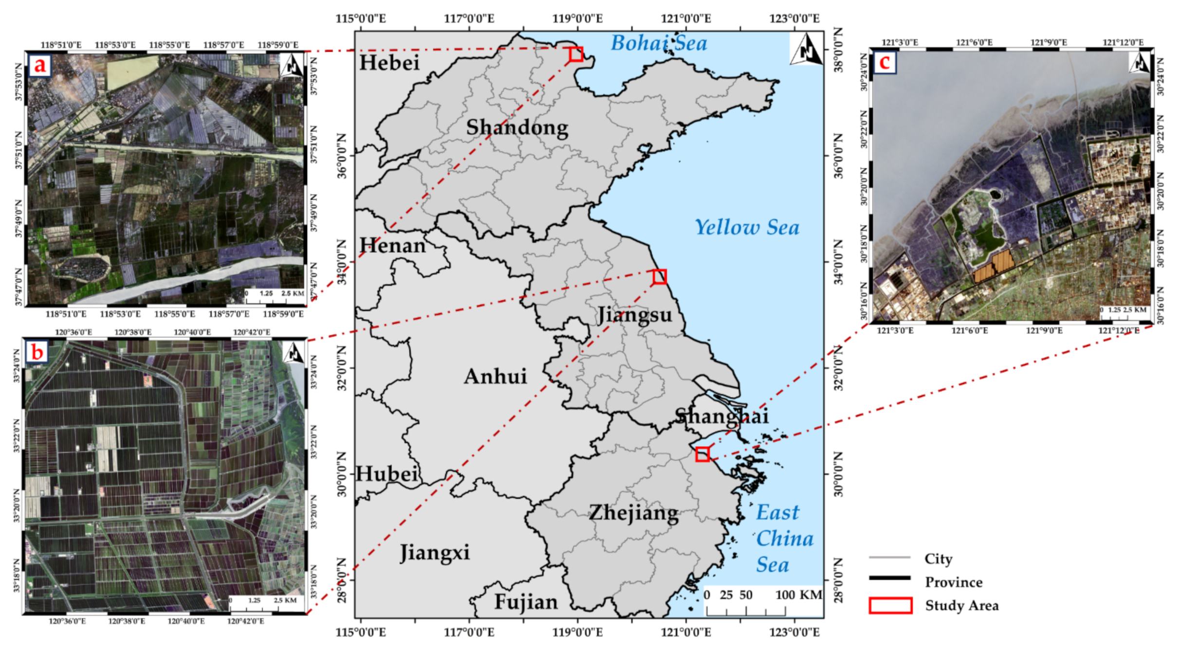
Coastal wetlands are located at the intersection of ocean and land, which are of great significance for resource protection, climate regulation, and maintenance of biodiversity, with impacts on carbon stocks. In addition, coastal wetlands are typical complex surfaces, which are significant challenges in achieving fine mapping [1]. Recently, remote sensing (RS) technology has grown up to be a key method for wetlands survey and monitoring. The increasing availability of RS data brings rapid advancement and interest in the field of radar and optical data fusion [2,3,4]. Satellite-based optical sensors passively receive solar electromagnetic waves reflected by ground objects for imaging with rich spatial and spectral information [5]. Among them, multispectral images typically have high spatial resolution and rich details [6,7]. Hyperspectral images are characterized by nearly continuous spectral information, which is a distinguishing and popular feature for classification tasks [8]. Synthetic Aperture Radar (SAR) is an active detector, and its imaging is not affected by meteorological conditions and sunlight levels [9,10]. Radar microwave is more sensitive to dielectric properties and moisture characteristics, and the cross-polarization of SAR has a fair degree on distinguishing the vegetation canopy [11,12]. SAR can also provide backscattering properties that are different from optical, such as the geometric structure and surface roughness [13,14,15,16]. Therefore, how to perform pixel-level fusion of optical and SAR images, integrating the high spatial-spectral resolution with the characteristics of polarized backscattering, is of great significance for coastal wetlands mapping.

Due to the uncertainties inherent in the data sources, common SAR and optical image fusion techniques can be divided into three categories: SAR and multispectral image fusion, SAR–panchromatic–multispectral image fusion, and SAR–hyperspectral image fusion. The fusion of SAR and multispectral images has been applied to earth with good results. Wu et al. used the shear wavelet transform to fuse TerreSAR-X images (3 m) with Landsat-8 multispectral images to enhance the extraction of impervious surfaces [17]. Yin and Jiang made a special calculation on SAR images to minimize distortion in spectral information when fused RADARSAT-2 (PolSAR) with Landsat TM images [18]. Gaetano et al. used the registered optical data as a guide map to Sentinel-1 SAR denoising by a generalized bilateral filter, then fused SAR with Sentinel-2 MS data to improve the accuracy of land use classification [19]. Shao et al. combined the intensity–hue–saturation (IHS) fusion technique with gradient transfer (GTF) algorithms and described the fusion of SAR and multispectral images as an optical image optimization process that better preserved radiation information and spatial details [20]. Amarsaikhan et al. improved the results of land cover classification based on wavelet transform fusion—high-resolution SAR and optical images were used as the research data—and then compared the fusion results with Brovey transform, Ehlers fusion, and PCA algorithms [21]. Kulkarni et al. proposed a method combining PCA with the DWT algorithm [22], and Chen et al. proposed an algorithm using generalized IHS combined with wavelet transform, both reducing the spectral distortion of multispectral images [23]. Yang et al. used the Gram–Schmidt algorithm to fuse GF-1 (WFV) multispectral images with Radarsat-2 PolSAR images, improving the classification results of coastal wetlands in the Yellow River Estuary and increasing the accuracy of extracting mudflats and reeds [24].

The fusion of SAR, panchromatic, and multispectral images has also been explored in depth. Byun et al. provided two fusion ideas for SAR, panchromatic and multispectral images. The first is an area-based hybrid pansharpening fusion scheme. The SAR image is divided into active and inactive regions, and different fusion rules are designed for the two regions. The AWT algorithm is used to fuse the SAR and the panchromatic image, and then the multispectral image has component substitution applied to fusion images [25]. The second is a texture-based fusion scheme. The local statistical parameters are adaptively calculated to perform a weighted fusion of panchromatic images and SAR. The multispectral images are fused with the generalized IHS transform [26]. Garzelli used à-trous wavelet transform to fuse panchromatic and multispectral images, then injected structural information from SAR images into the pansharpened images to obtain the final fusion results [27]. Yonghonga extracted the high-pass details of SAR and panchromatic images by á-trous wavelets, and the panchromatic detail information was modulated by texture HPFM (high-pass filter modulation) of SAR images and then fused with multispectral images, and the fused images have spectral fidelity in vegetation, bare ground, and buildings [28].

In recent years, with the great potential of hyperspectral analysis in wetland monitoring being explored, research on SAR and hyperspectral image fusion has emerged [29,30,31,32]. Chen et al. performed the IHS transformation to fuse hyperspectral data and Topographic Synthetic Aperture radar (TOPSAR) and obtained high spectral and spatial resolution images, solving the fuzzy classification of land cover [33]. Nasrabadi used the nonlinear correlation between SAR and hyperspectral images to fuse and perform the Reed–Xioli (RX) anomaly detector based on kernel learning, improving the accuracy of mine identification [34]. Dabbiru et al. fused UAV synthetic aperture radar (UAVSAR) and hyperspectral images (HSI) from an airborne visible/infrared imaging spectrometer (AVIRIS) to improve the classification of oil-contaminated coastal vegetation [35].

Overall, the fusion of optical and SAR images can integrate the rich spatial and spectral information of optical images, as well as the backscattering polarimetric properties of SAR, which is of great significance for the fine mapping of coastal wetlands. However, available fusion methods for optical and SAR images have the following problems that need to be solved urgently: (1) On the one hand, SAR and optical images have divergent imaging mechanisms, and their image properties are quite different; the fusion is extremely likely to result in information distortion and component destruction. (2) On the other hand, coastal wetlands are typically a complex surface, which further poses a greater challenge to the collaborative fusion of the optical and SAR images. (3) In addition, the existing pixel-level fusion methods mainly focus on the synthesis of SAR and multispectral (or panchromatic) images, and there are few studies on the fusion of SAR and satellite hyperspectral images, especially for multi-sensor optical and SAR image fusion. To the best of our knowledge, there are no integrated cross-modal pixel-level fusion methods for SAR, multispectral (MS), and hyperspectral (HS) images, which are promising by combining their complementary advantages for coastal wetlands mapping.

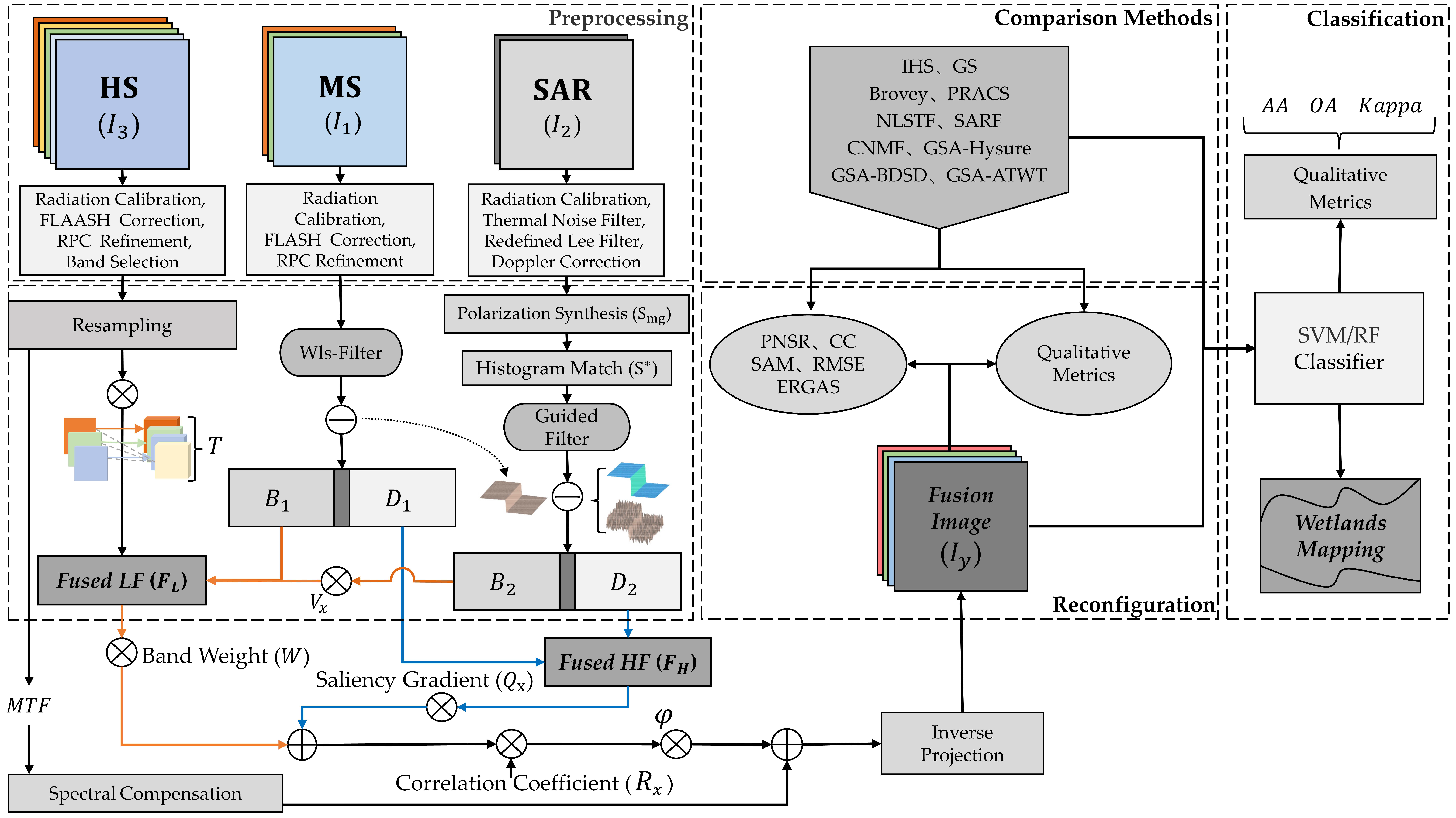
In view of the above problems, this paper proposes a multi-resolution collaborative fusion method of MS, HS, and SAR images to obtain high-quality images for practical applications, such as coastal wetland mapping. First, the high spatial resolution images are decomposed based on edge-preserving filters, reducing the information distortion by simultaneous positioning in the spatial and frequency domain. Secondly, to make the algorithm more robust, we design optical and SAR cross-modal weight in both spatial and spectral dimensions among the fusion branch, while weighted inverse projection is performed to provide good local fidelity. Finally, the upsampled HS images are modulated by injecting spatial detail information and backscattering polarimetric properties without disturbing spectral components. The main innovations of this paper are as follows:

• This paper firstly proposes a multi-modal collaborative fusion method for SAR, MS, and HS images to obtain the fused image with high spatial resolution, abundant spectral information, and the geometric and polarimetric properties of the SAR;
• In the proposed M2CF, the optimal spectral-spatial weighted modulation and spectral compensation are designed to reconstruct the high-fidelity fusion images. Furthermore, the backscattering gradients of SAR are guided to fuse, which is calculated from saliency gradients with edge-preserving, making it more suitable for cross-modal fusion with complex surface features;
• Fusion yields steady visible benefits, achieving the minimum spectral loss with high PSNR while robustly improving the classification results in coastal wetlands.

The rest of the paper is arranged as follows. Section 2 focuses on the methodological framework of the paper. Section 3 describes image preprocessing and the fusion datasets. Section 4 evaluates the fused images in terms of quantitative and qualitative metrics, and the classification accuracy is used to characterize the competitiveness of the fused images in realistic applications. Section 5 draws the discussion, and Section 6 presents the conclusions of our paper.

2. Methodology

2.1. Framework Description

Multi-resolution analysis (MRA) framework can locate in multi-frequency dimensions with spatial and spectral separation, reducing the spectral distortion in the fusion of optical images [36,37]. It is widely used and promoted because of its efficiency and portability, such as the fusion of infrared and visible images [38]. More remarkably, the MRA-based fusion images can obtain a better signal-to-noise ratio, which is beneficial for classification. In addition, it also can be used for extensive area, in-orbit, and multi-modal fusion without bringing the computational load. That is, MRA makes it possible to achieve the best fusion performance in multiple modalities.

The remote sensing image can be processed by MRA segmentation to obtain low-frequency and high-frequency components. The high-frequency component represents the texture details of the original image, mainly containing spatial information [39]. The low-frequency component is the base layer after filtering, which mainly contains spectral information [40]. The mathematical formula for MRA can be expressed as:

$$I_x=\alpha \times \left[B_x+D_x\right]+\beta$$

(1)

where $\alpha$ is the scaling factor of pixel values, and $\beta$ is the error term. $I_x\in {ℝ}^{d_x\times N}$ represents the unfolded matrix of a three-dimensional digital image with $d_x$ channels by $N$ pixels. $X$ is the number of modalities, ${\left\{I_x\right\}}_{x=0}^X$. $B_x\in {ℝ}^{d_x\times N}$ represents the low-frequency component of the filtered image, i.e., the base layer of the image; $D_x\in {ℝ}^{d_x\times N}$ represents the high-frequency component of the original image after MRA segmentation, which is obtained by the difference between the original image and the low-frequency component.

The traditional MRA framework is not suitable for fusion tasks with multi-modal or heterogeneous images, which are highly dependent on correlation between modalities. To enhance the integration ability of multi-modal images and reduce information loss, we proposed a multi-resolution collaborative fusion algorithm. Figure 1 illustrates a general flowchart of the multi-modal MRA collaborative fusion (M2CF) method. The core idea of this fusion algorithm is to decompose the remote sensing image based on the generalized multi-resolution analysis framework by applying edge-preserving filtering. Among them, we locate the spatial and spectral dimensions of the multispectral image and the de-speckle SAR image, and decompose the image into low-frequency (spectral) and high-frequency (spatial) components. The histogram-matched low-frequency and high-frequency components are weighted, and the subimages are collaboratively fused and reconstructed according to the MRA inverter. Finally, we perform spectral compensation on the reconstructed image to obtain the final fusion image. Accordingly, we describe some important steps of M2CF in detail below.

2.2. Multi-Frequency Extraction of MS

Edge-preserving (EP) filters are widely used in natural image enhancement and fusion. EP filters can be constructed by simple linear or multiple nonlinear filters. Typical EP filters are fast bilateral filters (FBF), weighted least squares filters (WlsF), guided filters (GF), etc. The WlsF was first proposed by Farbman et al. [41] and has become increasingly extensively employed in natural image processing. Recently, the WlsF has also been applied to image denoising, image tone modulation, and image detail enhancement. It is characterized by the ability to multi-scale tone and edge detail manipulation when the image is decomposed.

In this paper, we use the WlsF-based optimization framework to decompose the multispectral images into smooth and edge parts, respectively. The principle is to ensure that the basic gradient of the image remains unchanged. The filtered and smoothed image $B_1$ is like the input MS image $I_1$, in terms of spectral information and has distinct edge features. The filter model can be expressed as:

$$min\left[\parallel I_1-B_1{\parallel }_F^2+\lambda \times f_{\nabla }\left(I_1\right)\times \parallel I_1{\parallel }_F^2\right]$$

(2)

where $\lambda$ is a smoothing factor. $f_{\nabla }\left(I_1\right)$ is the image gradient of $I_1$, obtained by second-order derivatives. Then, the filter model is also calculated in the least square:

$$min{\displaystyle \sum }_k{\left(I_{1,k}-B_{1,k}\right)}^2+min{\displaystyle \sum }_k\lambda \left(a_{z,k}\left(B_1\right){\left(\frac{\partial I_1}{\partial z}\right)}_k^2+a_{t,k}\left(B_1\right){\left(\frac{\partial I_1}{\partial t}\right)}_k^2\right)$$

(3)

where the subscript $k$ represents the spatial location of the pixel. The weight coefficients of the smoothing term are $a_z$, $a_t$, and the subscripts indicate direction. The first term of the function represents the difference between the input and output image. The second term is the regular term, which makes the output image smoother by minimizing the bias derivative. The definition of the weight coefficients is:

$$a_{z,k}\left(I_1\right)={\left({\left|\frac{\partial Log\left(\mathcal{\ell }\right)}{\partial z}\left(k\right)\right|}^{\delta }+\epsilon \right)}^{-1}$$

(4)

$$b_{t,k}\left(I_1\right)={\left({\left|\frac{\partial Log\left(\mathcal{\ell }\right)}{\partial t}\left(k\right)\right|}^{\delta }+\epsilon \right)}^{-1}$$

(5)

where $log\left(\mathcal{\ell }\right)$ is the log value of the input image intensity band $\mathcal{\ell }$. The exponent $\delta$ (typically between 1.2 and 2.0) determines the sensitivity to the gradients of $I_1$. $\epsilon$ is the residual difference. The filtered image $B_1$ can be expressed as a linear matrix equation.

$$B_1=f_{\lambda }\left(I_1\right)={\left(I_{x_0}+\lambda L_k\right)}^{-1}\times I_1$$

(6)

where $B_1$ is obtained by applying a nonlinear operator $f_{\lambda }\left(·\right)$, which depends on the gradients of $I_1$. $I_{x_0}$ is an identity matrix. $L_k$ is a five-point spatially inhomogeneous Laplacian matrix obtained by minimizing the partial derivatives of $I_1$.

2.3. Multi-Frequency Extraction of SAR

SAR images also have different bands, like optical images, such as vertical send and vertical receive (VV) polarization, vertical send and horizontal receive (VH) polarization, etc. However, the polarization modes of SAR are distinctly different from the optical bands. In order to achieve complementary information between different polarization of SAR images while standardizing SAR images and reducing noise, polarization synthesis of SAR is required. Then, to deconstruct SAR and acquire continuous detail information, we use a guided filter (GF), which is more suitable for SAR multi-frequency extraction.

2.3.1. Polarization Synthesis

The polarization modes of SAR images are normalized in the range of $m$ to $n$:

$$\tilde{S}=\frac{\left(m-n\right)\times \left(S-S_{min}\right)}{S_{max}-S_{min}}$$

(7)

where $S_{min}$ is the minimum value of pixels in a SAR polarization, and $S_{max}$ is the maximum value of pixels in a SAR polarization. The polarization synthesized SAR image ${\mathrm{S}}_{mg}$ can be expressed by the following equation:

$$P=\left\{\begin{array}{c}{p}_1=1, p_2=0; v{v}_{ij}=max\left\{v{v}_{ij} ,v{h}_{ij}\right\}; \\ p_2=1, p_1=0; v{h}_{ij}=max\left\{v{v}_{ij} ,v{h}_{ij}\right\};\end{array}\right.$$

(8)

$${\mathrm{S}}_{mg}=p_1\times {\tilde{S}}_{vv}+p_2\times {\tilde{S}}_{vh}+\overline{S}$$

(9)

where $p_1$ is the position weight map of the pixel $v{v}_{ij}$ with a stronger backscattering value in VV polarization above all polarization bands. Similarly, $p_2$ is the position weight map of the pixel $v{h}_{ij}$ with a stronger backscattering value in VH polarization above all polarization. $\overline{S}$ is the mean value of the polarization bands at a certain pixel position.

In addition, the SAR image is a grayscale image, which needs to be matched with the optical image histogram. The standard deviation ${\sigma }_2$ of the SAR matrix can be calculated from the pixel values:

$${\sigma }_2=\sqrt{\frac{{\sum }_{i=1}^N{\left(S_i-{\overline{S}}_{mg}\right)}^2}{N}}$$

(10)

where the number of SAR pixels is $N$, $S_i$ is the i-th pixel of the SAR matrix $i\in \left[1,N\right]$, and ${\overline{S}}_{mg}$ denotes the pixel average of the SAR matrix. Histogram matching of the SAR image matrix is expressed as:

$$S^{*}=\left(S-{\overline{S}}_{mg}\right)\times \frac{{\sigma }_3}{{\sigma }_2}+{\overline{I}}_3$$

(11)

Similarly, ${\sigma }_3$ is the standard deviation of the HS image and ${\overline{I}}_3$ is the pixel average of the optical image. $S^{*}$ is the SAR matrix after histogram matching.

2.3.2. Guided Filter

The guided filter is a non-iterative filter, which belongs to the fast filter. In addition to the speed advantage, which can maintain the image gradient excellently [42], the important assumption of the guided filter is that there is a local linear relationship between the guided image and the output image within the filtering window. Meanwhile, according to the idea of MRA, the input image is composed of the base layer $B_2$ and details layer $D_2$ with spatial, sharp, texture, etc. Therefore, there are:

$$B_{2,i}=a_k{G}_i+b_k, \forall i\in {\omega }_k$$

(12)

$$B_{2,i}=S_i^{*}-D_{2,i}$$

(13)

where $k$ is the midpoint of the local window, so the pixels belonging to the window ${\omega }_k$ can be calculated using the corresponding pixels transformed by the coefficients of $(a_{k,}{b}_k)$. $S_i^{*}$ indicates the value of the input SAR matrix at position $i$; $G_i$ is the optical guided map; $B_{2,i}$ is the output matrix after guided filtering. Here, the output image can be considered as a local linear transformation of the guided map $G_i$. In order to maintain the local linear model and minimize the value difference between the input and output images in the local window, the equation can be expressed as:

$$\begin{gathered} \min {\displaystyle \sum }_{i\in w_k}{\left(S_i^{*}-B_{2,i}\right)}^2 \\ argmi{n}_{a,b}{\displaystyle \sum }_{i\in w_k}{\left(S_i^{*}-a_k{G}_i-b_k\right)}^2 \end{gathered}$$

(14)

Then, linear ridge regression is used with regularization parameters to fit the loss function:

$$J\left(a_k,b_k\right)=argmi{n}_{a,b}{\displaystyle \sum }_{i\in {\omega }_k}\left({\left(S_i^{*}-a_k{G}_i-b_k\right)}^2-ϵa_k^2\right)$$

(15)

where, $ϵ$ is the regularization parameter to prevent the value of $a_k$ from being too large. Solving the above equations yields the value of a and b at the guiding window as follows:

$$a_k=\frac{\frac{1}{\left|\omega \right|}{\sum }_{i\in {\omega }_k}\left(S_i^{*}\times G_i-{\overline{B}}_{2,i}\times {\overline{G}}_k\right)}{{\sigma }_k^2+ϵ}$$

(16)

$$b_k={\overline{S}}_k^{*}-a_k{\overline{G}}_k$$

(17)

where ${\sigma }_k$ is the standard deviation of the guiding image $G_k$ over the window ${\omega }_k$. ${\overline{S}}_k^{*}$ is the mean value of the SAR pixels within the filtering window. ${\overline{G}}_k$ is the mean value of the guided image within the filtering window. After obtaining the above equation, a pair of $(a_{k,}{b}_k)$ coefficient can be calculated for each filtering window.

However, each pixel is contained in multiple operation windows, and thus multiple $(a_{k,}{b}_k)$ can be computed for each pixel position. Where the value of the output image is obtained by the mean value of the coefficients, and the above process can be described as:

$$B_{2,i}=\frac{1}{\left|{\omega }_k\right|}{\displaystyle \sum }_{k,i\in {\omega }_k}\left(a_k{G}_i+b_k\right)$$

(18)

$${\overline{B}}_{2,i}={\overline{a}}_i{G}_i+{\overline{b}}_i$$

(19)

where ${\overline{a}}_i$ and ${\overline{b}}_i$ are the mean values of the coefficients calculated for all windows at the i-th pixel position, respectively.

2.4. Weight Configuration

Fusion weights of the spectral and spatial components are calculated separately. The hyperspectral image is selected for the primary spectral information after upsampling. It is modulated with two low-frequency components according to the correlation coefficient weight and the spectral transformation weight. For the high-frequency fusion branch, we apply pixel saliency gradient and spatial information ratio to fuse spatial information. The following subsections describe the details of the process.

2.4.1. Correlation Coefficient Weight

In the spectral information fusion branch, in order to avoid spectral distortion, it is necessary to find the fusion band of a certain MS image corresponding to the HS image. We find the corresponding fusion interval by calculating the correlation coefficient. The covariance matrix is expressed as $C\left(·\right)$, and then the correlation coefficient weight $R$ can be found at:

$$R\left(x_1,x_2\right)=\frac{C\left(I_{x_1},I_{x_2}\right)}{\sqrt{C\left(I_{x_1}\right)\times C\left(I_{x_2}\right)}}$$

(20)

where $I_x$ are the independent variable matrices. $R\in \left(0,1\right]$, the higher value of $\left|R\right|$, the closer relationship between the two spectral matrices.

2.4.2. Saliency Gradient Weight

The visual weight map (VWM) based on saliency extraction is mainly used for image fusion under multi-scale decomposition. The saliency gradient is used to design a visual weight map, which defines the visual importance of each pixel. Pixel locations with a larger VWM value usually correspond to the edge and texture areas, and these areas often contain richer spatial features. The intensity contrast between different pixels of the image is used to extract the saliency gradient. The pixel range of the image matrix $I_x$ is $\left[m,\mathrm{n}\right]$, then the saliency gradient is $V_x\left(q\right)$:

$$V_x\left(q\right)={\sum }_m^{n}Cq\times \left|I_{x,k}-I_{x,q}\right|$$

(21)

where $Cq$ denotes the number of pixels where the pixel value is $q$, $\forall q,k\in \left[m,n\right]$. The locations of the pixel with larger values on the visual weight map usually correspond to edge and texture regions. We sum the visual weight values of all pixels and take the mean value ${\overline{V}}_{x_1}$. It can be approximated as the richness of the spatial information and is used to calculate the fusion weight of the image spatial detail.

$${\overline{V}}_{x_1}={\sum }_m^n\frac{V\left(q\right)}{N}$$

(22)

$$Q_{x_1}=\frac{{\sum }_m^n\frac{V\left(q\right)}{N} }{\sum V_x}$$

(23)

where ${\overline{V}}_{x_1}$ denotes the average visual weight value of the image matrix with the number of $N$ pixels, and $V_x$ is the x-th visual weight matrix. The saliency gradient weight of the image matrix $x_1$ is defined as $Q_{x_1}$.

2.4.3. Hyperspectral Band Weight

The spatial information ratio between different bands of the HS image is precisely proportional to its spatial optimization effect on the fused image. The intensity component of the HS image is calculated (the average of all bands is usually considered as the intensity value). Then, the ratio of the standard deviation of each hyperspectral band ${\sigma }_{3,i}$ to the intensity band ${\sigma }_{3,\mathcal{\ell }}$ is calculated. This ratio is used as the band weight W of HS images, it is defined as:

$$W=\frac{{\sigma }_{3,i}}{{\sigma }_{3,\mathcal{\ell }}}$$

(24)

2.4.4. Spectral Transformation Weight

MS data can be considered as the spectral degradation of HS data. The multispectral image $I_1$ is correlated with the hyperspectral image $I_3$ by:

$$argmi{n}_T\parallel I_3-T\times I_1+e{\parallel }_F^2$$

(25)

where $\parallel ·{\parallel }_F$ is the Frobenius norm of the matrix. $T\in {ℝ}^{d_1\times d_3}$ denotes the spectral transformation matrix, e is the spectral residual. Each channel vector ${\left\{T_i\right\}}_{i=1}^{d_3}$ represents the spectral transformation matrix of the i-th HS band to multispectral image [43]. Then, the spectral transformation function can be fitted by the least square:

$$argmi{n}_T\sum {\left(I_{3,i}-T_i\times I_{1,i}+e\right)}^2$$

(26)

2.5. M2CF: Multi-Modal MRA Collaborative Fusion

Table 1. Description of variable symbols.

Notation	Description	Dimensions
$I_x$	The x-th remote sensing image.	$d_x\times N$
$B_x$	Low-frequency components of the original image.	$d_x\times N$
$D_x$	Obtained by the difference between the $I_x$ and $B_x$.	$d_x\times N$
$\parallel A{\parallel }_F$	The Frobenius norm of $A$, $\parallel A{\parallel }_{\mathrm{F}}=\sqrt{\mathrm{tr}\left(A^{T}A\right)}$.	$1\times 1$
$\tilde{S}$	The normalized SAR images, obtained by Equation (7).	$1\times N$
$S^{*}$	SAR under synthesized and histogram matched.	$1\times N$
$R_x$	The correlation coefficient, obtained by Equation (20).	$d_x\times d_3$
$V_x$	Visual weight of the x-th image matrix.	$1\times N$
$Q_x$	Saliency gradient weight of the x-th image matrix.	$1\times 1$
$W$	Band weight of the hyperspectral image.	$d_3\times 1$
$T$	Spectral transformation weight for MS image.	$d_1\times d_3$
$f_{up }\left(I_x\right)$	Indicates upsampled $I_x$ image.	$d_x\times N$
$\phi$	Spatial penalty term to balance the equation.	$1\times 1$
$g_l/g_h$	The fusion coefficients of subimages.	$1\times 1$
$I_y$	The final fusion image after spectral compensation.	$d_3\times N$

gives the symbols and descriptions of the variables used in the proposed M2CF method. In the table below, the subscripts $x\in 0,1,2,3$. $I_1$, $I_2$ and $I_3$ represent the MS, SAR, and HS image, respectively. $I_0$ is a zero matrix of the same size as the hyperspectral image. $I_{\mathcal{\ell }}$ is the identity matrix.

The modalities after multi-resolution decomposition are integrated according to the fusion weight based on the multi-resolution analysis inversion. Fusion rules are very important but difficult. Here, the low-frequency component $F_L$ and the high-frequency component $F_H$ of the fused image can be obtained by the weighting operation:

$$F_H=I_0+g_{h}W\times \left[Q_x\times R_x\times D_x\times \left(1+V_1\right)\right],x\in 1,2$$

(27)

$$F_L=f_{up }\left(I_3\right)+g_{l}W\times \left[\left(T+R_1\right)\times B_1+R_2\times B_2\right]$$

(28)

where $g_l$ and $g_h$ are the fusion coefficients of low-frequency and high-frequency information, respectively. $Q_x$ is the saliency gradient weight. $f_{up }\left(\cdot \right)$ indicates upsampling operation. $I_0$ is a zero matrix of the same size as the HS image after upsampling. Then, the preliminary fusion image $Y$ can be represented as:

$$Y=F_L+\phi F_H$$

(29)

where $\phi \in \left(0,1\right]$ is the spatial penalty term to balance the importance of different terms.

However, inverse reconstruction inevitably produces spectral residuals. Meng et al. introduced the concept of spectral compensation to improve the spectral fidelity [44]. Similarly, we obtain the spectral compensation matrix by calculating the difference between the original low-resolution hyperspectral image and the preliminary fused image, and then the spectral loss of the fused image is compensated. The spectral compensation process can be expressed as:

$$I_y=Y+f{\left[I_3-f_{\mathrm{down} }\left(f_{\mathrm{MTF} }\left(Y\right)\right)\right]}_{up}$$

(30)

where $f_{MTF}\left(\cdot \right)$ and $f_{\mathit{down} }\left(\cdot \right)$ denote MTF blurring and down-sampling, respectively. $I_3$ is the low-resolution hyperspectral image. $I_y$ denotes the final fused image.

3. Study Area and Datasets

3.1. Study Area

Owing to the complicated and heterogeneous distribution of wetland features, the coastal wetlands are also known for their typically complex and challenging surfaces. The study area includes the Yellow River Estuary, Yancheng, and the South Shore of Hangzhou Bay coastal wetlands (Figure 2). These wetlands are often used as study areas for hyperspectral image processing or wetland mapping [24,45,46,47,48]. The Yancheng is in the east of Jiangsu Province, China. It is a typical silty mudflat coast, the largest coastal wetland on the edge of the Asian continent. The study area has formed a complex wetlands ecosystem and mainly contains salt marshes, culture ponds, and natural vegetation. The Yellow River Estuary, an alluvial delta plain formed by the accumulation of river sediment, is in the northeast of Shandong Province, China. There is an ecological protection area with a national nature reserve. It has abundant resources, and mainly contains paddy fields, potholes, and reeds. The Hangzhou Bay National Wetland (Hangzhou Bay for short) is in the northwestern part of Hangzhou Bay, Zhejiang Province, China. The wetland is rich in flora and fauna with numerous semiaquatic plants, such as Spartina alterniflora, Tamarix, Suaeda salsa, etc.

3.2. Preprocess and Datasets

In this fusion experiment, ZY-1 02D and GaoFen-5B (AHSI) hyperspectral images, Sentinel-2 and GaoFen-5B VIMI multispectral images, and Sentinel-1A SAR are multi-resolution RS datasets. The European Space Agency (ESA) provides worldwide Sentinel Series RS data services (https://scihub.copernicus.eu (accessed on 1 February 2022)). Gaofen-5 provides 30 m ground sample distance, 5 nm spectral resolution with 150 bands in VNIR (400–1000 nm), and 10 nm spectral resolution with 180 bands in short-wave infrared (1000–2500 nm). The acquisition dates or satellite perigee passing time of Sentinel-1A SAR and optical images are nearly identical, which ensures that the ground type remains unchanged. Sentinel-1A SAR offers a dual polarization mode with short revisit times. We selected four 10 m spatial resolution bands in Sentinel-2A, including three visible bands and a near-infrared band.

SAR images are preprocessed in Sentinel Application Platform (SNAP) 6.0, mainly including thermal noise removal, terrain correction, and de-speckle. Among them, the SAR artificial de-speckle filter is used to suppress the noise in homogeneous regions and improve the edge features. Here, the Redefined Lee filter is chosen to remove the speckle noise with a window size of 5 × 5. The final resampled SAR image has 10 m spatial resolution with 1500 × 1500 or 1800 × 1800 pixels (

Table 2. Specific information of the experimental datasets.

Experiment Datasets	Acquisition Date (UTC + 08:00)	Sensors	Mode	Spatial Resolution	Dimensions	Bands
Yan Cheng	6 September 2020 10:56	ZY-1 02D	HSI	30 (m)	500 × 500	147
	5 September 2020 10:35	Sentinel-2B	MSI	10 (m)	1500 × 1500	4
	9 September 2020 17:54	Sentinel-1B	SAR	10 (m)	1500 × 1500	2
Yellow River Estuary	28 June 2020 11:08	ZY-1 02D	HSI	30 (m)	500 × 500	117
	28 June 2020 10:55	Sentinel-2A	MSI	10 (m)	1500 × 1500	4
	28 June 2020 18:05	Sentinel-1A	SAR	10 (m)	1500 × 1500	2
Hangzhou Bay	29 December 2021 10:39	GF-5B AHSI	HSI	30 (m)	600 × 600	210
	29 December 2021 10:39	GF-5B VIMI	MSI	20 (m)	900 × 900	6
	27 December 2021 17:55	Sentinel-1A	SAR	10 (m)	1800 × 1800	2

). Optical images are preprocessed based on ENVI 5.3, mainly including radiometric calibration and the Fast Line-of-Sight Atmosphere (FLAASH) correction. The global digital elevation model (DEM) data at 30 m was used to correct the optical and SAR images (https://asterweb.jpl.nasa.gov/gdem.asp (accessed on 14 December 2021)). Then, the Global Digital Elevation Model (DEM) is applied to the surface reflectance products for orthorectification correction. HS images also require eliminating the bad bands, including overlapping bands, blurred or damaged bands, etc. Accurate registration, a process of geometric alignment of SAR and optical imagery, is the foundation of image fusion. Manual selection of control points on the SAR and optical images is laborious and time-consuming, and it is difficult to calibrate the corresponding points between different modalities [49]. To address the above issues, the following registration process is designed for cross-modal images: The preprocessed Sentinel-2 MS image is used as the reference image. The SAR and HS images are registered separately from the reference image. In this way, the multi-modal registration is reduced to optical registration and Sentinel series registration. Among them, the control points are artificially assisted to realize the coordinated registration. We selected the geometric angle and boundary as reference points and apply the registration module in the ENVI5.3 to alignment. The registration accuracy of the experimental datasets approaches the sub-pixel level (RSE ≈ 0.34).

3.3. Sample Selection and Distribution

To evaluate the performance of fused images for practical applications, we perform further classification experiments on three coastal wetlands. The random forest (RF) classifier as an ensemble learning algorithm and the support vector machines (SVM) classifier as a machine learning algorithm both have been widely used for RS image classification. Among them, the SVM and RF classifiers coded in MATLAB^®2020a are used for the experiments. The SVM classifier adopts the radial basis function as the kernel function, and the variance parameter and penalization factor are estimated via cross-validation. The number of decision trees in the RF classifier is manually set to 500. The main reason for choosing two classifiers is that we expect to see a performance gain due to the fusion algorithm rather than the advanced classifier. We obtained the region of interest (ROI) for all feature classes by using high-resolution Google Earth, field sampling, and according to careful image interpretation (Figure 3). Except for image preprocessing and registration, all image processing steps were performed by MATLAB^®2020a coding, including image fusion, evaluation metrics, and classification.

4. Experimental Results

In order to verify the effectiveness of the proposed method, we conducted fusion experiments on real RS images and compared quantitative metrics with several classical fusion algorithms. These include component substitution methods, model-based methods, hybrid methods, etc. All the fusion codes were run on a WIN10 computer with an Intel Core i9 processor and 128 GB RAM. The running time (in seconds) was recorded to evaluate the computational efficiency. Further classification experiments were conducted to characterize the practical application capability of the fused images.

4.1. Image Fusion Results

In this part, we use real RS data to evaluate the fusion algorithms in a more objective and specific way. The Yancheng wetlands are rich in spatial detail, and the Yellow River Estuary and Hangzhou Bay wetlands have complex spectral information. Figure 4, Figure 5 and Figure 6 show the comparison of fusion results obtained by the proposed M2CF and other fusion algorithms. The main comparison methods include CS-based, MRA-based, tensor decomposition-based, hyperspectral super-resolution, unmixing-based, and hybrid methods [20,36,44,50]. In this, all fusion results are presented in true color with local zooms (Bottom right corner). The Wald protocol is addressed as a solution to the problem of reference image non-availability [51]. The consistency property indicates that any high-resolution fusion image should be as close as possible to the source image after down-sampling. Experiments using the original hyperspectral image as a reference and down-sampling the fused image to evaluate the spectral distortion.

Table 3. Evaluation metrics of different fusion methods in Yancheng.

Fusion Methods	Quantitative Metrics					Running Time
	PSNR	SAM	CC	RMSE	ERGAS
IHS	23.6280	9.6515	0.7155	0.04242	38.5805	68.9314
GS	23.7360	11.8058	0.7459	0.04789	38.1233	119.6040
Brovey	23.5187	8.9363	0.7634	0.04641	35.1931	868.6111
PRACS	24.9276	5.4016	0.76366	0.27632	84.9932	1030.0152
CNMF	25.9117	5.1363	0.8664	0.03635	26.6683	1472.3720
NLSTF	31.5899	4.6968	0.9792	0.01721	14.7011	700.5636
SARF	28.7493	6.2618	0.9629	0.02574	27.1026	144.1752
GSA-Hysure	23.6181	10.1104	0.8377	0.04544	38.4659	3686.5776
GSA-BDSD	29.9061	7.8741	0.9677	0.02918	18.4949	295.5739
GSA-ATWT	32.4186	4.9149	0.9772	0.02110	13.4138	192.6265
M2CF (Proposed)	38.1668	2.5525	0.9938	0.01149	7.0877	355.8300

,

Table 4. Evaluation metrics of different fusion methods in Yellow River Estuary.

Fusion Methods	Quantitative Metrics					Running Time
	PSNR	SAM	CC	RMSE	ERGAS
IHS	17.9721	9.3361	0.4591	0.07252	43.9962	32.0599
GS	18.1503	9.4228	0.4497	0.07692	44.0660	47.2686
Brovey	17.8701	8.1697	0.4392	0.07590	44.2001	35.2524
PRACS	25.1538	3.5619	0.8404	0.18539	79.1565	1219.1587
CNMF	23.8400	3.6861	0.8306	0.04641	22.3898	1377.0568
NLSTF	28.3358	3.9234	0.9274	0.02911	13.0927	563.4189
SARF	19.2741	6.6625	0.8641	0.05676	25.2628	132.0532
GSA-Hysure	20.9068	5.1851	0.7879	0.05665	29.0530	2869.8089
GSA-BDSD	30.2073	3.2387	0.9757	0.02257	9.6567	255.6573
GSA-ATWT	30.5702	3.0832	0.9752	0.01888	9.3029	175.9395
M2CF (Proposed)	30.8864	1.9004	0.9782	0.01914	8.9354	138.6756

and

Table 5. Evaluation metrics of different fusion methods in Hangzhou Bay.

Fusion Methods	Quantitative Metrics					Running Time
	PSNR	SAM	CC	RMSE	ERGAS
IHS	29.8409	7.5310	0.8036	0.03450	27.2223	167.5567
GS	29.7873	4.1202	0.8206	0.02530	17.3417	129.8105
Brovey	29.6520	3.9635	0.8103	0.01618	17.3140	108.3487
PRACS	34.7274	5.7495	0.8289	0.02332	25.6469	1096.1787
CNMF	31.1619	9.3361	0.8440	0.02993	24.5317	2061.8031
NLSTF	31.6462	3.3214	0.9390	0.01790	10.3979	3982.5931
SARF	23.0536	7.1064	0.8842	0.08799	21.2838	297.1281
GSA-Hysure	35.8663	3.7498	0.9213	0.02050	12.2087	5982.9252
GSA-BDSD	37.6267	3.3107	0.9499	0.01678	7.2889	1445.8150
GSA-ATWT	39.5996	2.6122	0.9607	0.01526	9.8749	352.9102
M2CF (Proposed)	43.4879	2.5395	0.9732	0.01537	5.0824	285.8053

describe the quantitative metrics for image fusion methods, and the best one is shown in bold. Statistical quantitative evaluation metrics include the peak signal to noise ratio (PSNR), the spectral angle mapper (SAM), the correlation coefficient (CC), the root mean square error (RMSE), and the dimensionless global error in synthesis (ERGAS).

4.1.1. Fusion Results of Yancheng

Figure 4 shows that all fusion images are brighter than the original HS images in visualization. Traditional component substitution (CS) methods have improved spatial resolution compared to the reference image (ZY-1 02D). However, CS-based methods, such as IHS, GS, and Brovey have severe spectral distortions. Specifically, the muddy water in the upper right corner of the GS, Brovey, and PRACS has been distorted to purple on the true-color images. CNMF and GSA-Hysure (hyperspectral super-resolution) methods have severe spatial distortion. Constrained by the speckle noise of SAR, CNMF shows loss of texture information, while GSA-Hysure shows obvious radar noise. Although the combination of CS and MRA resulted in little spectral distortion, the GSA-BDSD and GSA-ATWT fusion images still retained noticeable speckle noise. The proposed M2CF method has minimal spectral distortion and significant spatial optimization compared to others.

Table 3 shows the robustness of the proposed method and GSA-ATWT in the spectral fidelity with spectral angle map (SAM) less than 5 and peak signal-to-noise (PSNR) ratio greater than 30. The conventional CS-based method has superior PSNR and short consumption time, but the spectral error is large. The CNMF and GSA-Hysure methods are not satisfactory. Although the SAM of the NLSTF fused result is smaller, the fusion image is blurry. In contrast, the SARF method has poorer spectral metrics, but it has better visualization compared to CS-based fusion. The M2CF achieves the minimum loss and has the best spectral fidelity with the effect of SAR noise cancellation while improving the spatial resolution.

4.1.2. Fusion Results of Yellow River Estuary

Figure 5 shows the original images and fusion results of all ten methods; Table 4 lists the quantitative metrics. This region is smooth with fewer spectral differences in features. The fusion results generally emerge from the polarimetric backscattering properties of SAR. Some bare lands are bright in the fused images, which have low spectral reflectance in the optical images, and the water potholes look darker. Traditional CS-based methods have severe spectral distortions, and hybrid methods produce spectral distortions on the individual feature class, except for the GSA-BDSD and GSA-ATWT. CS-based methods have some effects on cloud removal, such as the GS and IHS, where the intensity component from the upsampled HS data is unselectively replaced by the SAR, resulting in large differences in spectral information.

The fusion image of CNMF loses some optical details. SARF is not suitable for image fusion with a large number of bands. The reason for this is that SARF injects spatial details into HS data intensity components to maintain spectral fidelity. The fusion image generated by NLSTF is rather noisy since less spatial information is considered in models. GSA-Hysure performs image interpolation several times during the fusion process due to the mechanism of the algorithm, which involves more strange pixels and causes more significant spatial distortion. Fusion images of the hybrid method have less spectral distortion, but have less spatial improvement, which is poorly visualized.

The Yellow River Estuary RS image is smoother so that the PSNR of the fusion results is lower, and the spatial enhancement is generally poorer. Among the evaluation metrics of the fused images, the CS-based methods have the lowest PSNR, and the SAM is the largest. For the MRA-based GSA-BDSD, to ensure the robustness of the spectral fidelity, the injection weight of the high-frequency information is rationed less, and the injected spatial details are insufficient, which limits the spatial enhancement. The performance of the hybrid method is relatively good, and the M2CF method is the best.

4.1.3. Fusion Results of Hangzhou Bay

The spectral information (GF-5B) used in Hangzhou Bay is richer compared to the other two study areas, and the spatial resolution is progressive between modalities. Figure 6 shows that the spectral distortion of fusion images is smaller than in the previous areas, and the spatial optimization is weaker. It is noted that there is pseudo-noise at the intersection of ocean and land on the original SAR image. The CS-based methods and CNMF have large spectral distortions, and the pseudo-noise belonging to the SAR image is still clearly visible, mainly due to their inherent processing mechanism. SARF and hybrid methods reduce the approximation error while eliminating the speckle noise. GSA-Hysure, CNMF, and NLSTF generate new noise in the fusion process of pixel operations, and such methods are not suitable for the fusion of SAR and optical images. The fusion results of the hybrid method are darker than the original GF-5 HS image. Among them, although GSA-BDSD has no obvious SAR image artifacts, it still has a significant amount of speckle noise belonging to the SAR image. Figure 6 shows the robustness of GSA-ATWT, GSA-BDSD, and NLSTF in terms of spatial fidelity and underlines the potential of the proposed method.

Table 5 describes the quantitative metrics of eleven fused images in Hangzhou Bay. The CNMF method has the most severe spectral distortion. In addition, the running time of GSA-Hysure and NLSTF leave much to be desired. SARF has good visualization but poor quantitative metrics, which inject radar details into HS data with the variable gain coefficient.

According to the results from the three study areas, there is a basically identical trend in both quantitative and qualitative comparisons. CS-based methods have the least operation time but are highly dependent on the correlation between the source images. However, there are spectral mismatches between different sensors and divergent properties between modes, which can cause significant spectral distortion. The disadvantage of the PRACS method is that the dimensionless global error is large. The observations in Table 3, Table 4 and Table 5 show the robustness of GSA-ATWT, GSA-BDSD, and M2CF in terms of spectral fidelity. It is interesting that PRACS has good spectral fidelity in Hangzhou Bay, whereas it suffers serious spectral distortion in the Yancheng and Yellow River Estuary. Methods based on unmixing and hyperspectral super-resolution are prone to spatial texture detail distortion with a poor signal-to-noise ratio. NLSTF is prone to artifacts and a heavy computational burden. Apparently, hybrid methods are better than CS-based methods. Nevertheless, hybrid methods are not stable, and the algorithms are complex with long procedures. The flexibility and accuracy of the proposed M2CF are much better than that of hybrid methods. The proposed M2CF has the best fusion results; it promotes spatial resolution with high spectral fidelity. Experimental results show that the proposed method is more proper for fusing SAR, MS, and HS images.

4.2. Spectral Profiles Comparison

The reflectance at different wavelengths can be expressed in the image cube as a spectral profile. The pure pixel spectral profiles of three typical features are compared before and after the fusion (Figure 7), namely water, vegetation, and dry land/salt marsh. It can be found that the overall trend of the spectral profiles is correct and fits the original reference properly, especially in Hangzhou Bay. However, the profiles of the CS-based methods are mismatched in all three regions. Some fusion images even show negative values in the water profiles, such as the GS, Brovey, and NLSTF. The unmixing-based (CNMF) profile is mostly lower than the reference profiles in salt marshes and water. There is no regularity in the spectral profiles of the hybrid methods, and it fluctuates within a certain small range. Fortunately, including M2CF, the spectral profiles of GSA-BDSD and GSA-ATWT are high-fidelity on all four typical features, indicating that the spectral dimension was preserved well during the fusion process. Once again, the spectral fidelity of the proposed method is relatively robust.

4.3. Classification Results

To test the specific performance of the fusion methods, the fused images are employed for classification, and its application ability is characterized by the accuracy rate. The RF and SVM classifiers were trained 75 times, and then we computed three widely-used metrics for classification results, namely Overall Accuracy (OA), Average Accuracy (AA), and Kappa Coefficient. The classification accuracy was the mean value of 20 times to make a quantitative performance comparison. Classification metrics for HS images and optical (HS + MS) fusion images were included in the comparison to characterize the improvement in classification accuracy.

4.3.1. Classification Results of Yancheng

As can be observed, ZY-1 02D HS has the worst classification result, mainly due to the lower spatial resolution (Figure 8). In other words, HS has complete classification blocks, but the detail differentiation is weaker. The classification accuracy of most fusion images with high spatial and spectral resolution was enhanced. However, PRACS and CNMF fusion images are limited by the similarities in spectral reflectance. In the classification of the MRA-based hybrid fusion images, culture pond and salt marsh were easily misclassified. Among them, the BDSD fused image has many misclassified pixels in dry land and paddy field, and the boundaries in spartina alterniflora and reed are unclear.

Table 6. Classification metrics of Yancheng.

Method Index	RF			SVM
	AA	OA	Kappa	AA	OA	Kappa
ZY-1 02D	0.7624	0.8427	0.8182	0.7946	0.8601	0.8384
MS + HS	0.8565	0.8879	0.8716	0.9230	0.9495	0.9423
IHS	0.8138	0.9194	0.8992	0.9448	0.9736	0.9673
GS	0.8136	0.9112	0.8894	0.9412	0.9713	0.9643
Brovey	0.7710	0.9063	0.8830	0.8704	0.9174	0.8979
PRACS	0.8962	0.9421	0.8350	0.7751	0.9404	0.7972
CNMF	0.6847	0.8148	0.7695	0.7159	0.8035	0.7562
NLSTF	0.8526	0.8686	0.8628	0.9244	0.9474	0.9399
SARF	0.8342	0.8502	0.8420	0.9281	0.9540	0.9484
GSA-Hysure	0.8766	0.9375	0.9224	0.9410	0.9713	0.9643
GSA-BDSD	0.8635	0.9331	0.9172	0.9513	0.9759	0.9701
GSA-ATWT	0.7357	0.8808	0.8509	0.9127	0.9579	0.9478
M2CF	0.8972	0.9484	0.9359	0.9589	0.9775	0.9721

depicts the OA, AA, and Kappa of the classification in Yancheng. In quantitative metrics, the accuracy of the fusion images mostly exceeds that of images based on single ZY-1 02D data. However, CNMF has lower classification accuracy than optical fusion images in two classification experiments. Because of the spectral distortion results in CNMF fusion, misclassification occurs when combining spatial information. Among the accuracy metrics of the random forest classifier, the overall accuracy of Brovey, SARF, and GSA-ATWT is lower than optical fusion image, and all other methods improved to different degrees. PRACS has better accuracy in RF Classifier but is not as precise as ZY-1 02D in SVM Classifier.

Collectively, the proposed M2CF’s OA and Kappa were the highest among the metrics in the Yancheng, and the AA in the RF classification experiments improved about 9% over the classification results using HS alone; the OA and Kappa in the SVM experiments improved by 3.80% on average, further demonstrating that image fusion can improve the classification accuracy of the coastal wetlands. This reinforces the conclusion that the fusion of optical and radar data is indeed able to provide valuable synergistic information.

4.3.2. Classification Results of Yellow River Estuary

Figure 9 shows the RF and SVM classification results in the Yellow River Estuary, and

Table 7. Classification metrics of Yellow River Estuary.

Method Index	RF			SVM
	AA	OA	Kappa	AA	OA	Kappa
ZY-1 02D	0.7903	0.8719	0.8504	0.8563	0.9245	0.9118
MS + HS	0.8404	0.9163	0.9023	0.9385	0.9720	0.9674
IHS	0.8791	0.9313	0.9199	0.9487	0.9759	0.9719
GS	0.8750	0.9260	0.9138	0.9444	0.9735	0.9691
Brovey	0.8016	0.8576	0.8339	0.9107	0.9427	0.9332
PRACS	0.8793	0.9309	0.9195	0.8456	0.92275	0.9096
CNMF	0.8231	0.8876	0.8690	0.8750	0.9230	0.9103
NLSTF	0.8544	0.9144	0.9069	0.9437	0.9587	0.9569
SARF	0.8342	0.8602	0.8400	0.9281	0.9540	0.9474
GSA-Hysure	0.7483	0.8509	0.8257	0.8896	0.9432	0.9338
GSA-BDSD	0.8818	0.9366	0.9261	0.9407	0.9723	0.9678
GSA-ATWT	0.8566	0.9207	0.9075	0.9363	0.9715	0.9668
M2CF	0.8964	0.9426	0.9331	0.9542	0.9789	0.9754

lists quantitative metrics of the classification accuracy. Similarly, the M2CF method had better classification results. The SVM classifier shows PRACS, the hybrid method, and the proposed method visualize better, which is more consistent with the classification results of the Yancheng wetlands.

Visually, the HS image (ZY-1 02D) of the Yellow River Estuary has blurred classification on salt marshes and culture ponds in SVM classification experiments. It is observed that for the concerned application, both optical (MS + HS) and other fusion images are promising as compared to the ZY-1 02D HS, except for GSA-Hysure and PRACS. With the improvement of spatial resolution, the ability to distinguish the details was enhanced. The classification results of CS-based methods (e.g., Brovey and GS) are quite fragmented, mainly because the fused images retain the image details and speckle noise of the SAR. PRACS has no significant ability to make a distinction between paddy fields and culture ponds in both sets of experiments. The IHS and GS are misclassifications of the Yellow River in both classifiers, distinctly. For CNMF and GSA-Hysure methods, they fail to classify the materials well due to their sensitivity to complex noise (Figure 9). For the M2CF and three hybrid methods, the classification of salt marshes and culture ponds is differentiated well, which has similar spectral characteristics to optical images because SAR images are sensitive to soil moisture and geometric structure. However, the MRA-based hybrid methods are prone to speckle misclassification in Pothole.

The quantitative metrics of classification accuracy show that GSA-Hysure has lower classification accuracy than HS alone. It illustrates that inappropriate fusion algorithms can even reduce classification accuracy (Table 7). The classification accuracy of NLSTF and SAR is roughly the same as the optical fusion image (HS + MS). The best classification accuracies were achieved for the fused images obtained by the M2CF method, and the OA was improved by about 5% over the hyperspectral images alone. Again, proving the superiority of our proposed fusion method over other fusion methods. The classification experiments further illustrate that pixel-level fusion of SAR and optical images can improve classification accuracy, especially in the identification of water bodies, bare land, and vegetation. It indicates the importance of image fusion for coastal wetland mapping.

4.3.3. Classification Results of Hangzhou Bay

In general, the pixels are usually mixed on the low-resolution HS in Hangzhou Bay; it is observed that multi-modal image fusion improves the wetlands classification to some extent. Concretely, CNMF has mass misclassification of ocean and pothole, which pollutes the maps. Moreover, due to the noise interference, the performance of CS-based fusion image is not improved or even negative. The NLSTF is unsuitable for identifying the subspaces of data in complicated areas. Hybrid methods perform well with clearer classification maps, especially the textures between photovoltaic panels and artificial trenches. In RF Classifier, the accuracy of optical fusion (MS + HS) is higher than that of CNMF, SARF, and GSA-Hysure. The quality of image fusion is directly related to the accuracy and visualization of classification results. The classification accuracy is improved through the hybrid fusion methods (

Table 8. Classification metrics of Hangzhou Bay.

Method Index	RF			SVM
	AA	OA	Kappa	AA	OA	Kappa
ZY-1 02D	0.8549	0.9137	0.9021	0.8863	0.9331	0.9308
MS + HS	0.9041	0.9221	0.9219	0.9278	0.9464	0.9426
IHS	0.9167	0.9392	0.9356	0.9397	0.9532	0.9514
GS	0.9196	0.9472	0.9432	0.9411	0.9543	0.9532
Brovey	0.9212	0.9469	0.9428	0.9529	0.9620	0.9607
PRACS	0.9273	0.9435	0.9407	0.9377	0.9425	0.9410
CNMF	0.8368	0.9190	0.9047	0.8306	0.9184	0.9056
NLSTF	0.9298	0.9437	0.9392	0.9339	0.9514	0.9499
SARF	0.9205	0.9526	0.9461	0.9508	0.9689	0.9657
GSA-Hysure	0.9288	0.9489	0.9434	0.9419	0.9590	0.9571
GSA-BDSD	0.9282	0.9571	0.9528	0.9547	0.9616	0.9602
GSA-ATWT	0.9375	0.9611	0.9583	0.9515	0.9636	0.9619
M2CF	0.9411	0.9675	0.9650	0.9550	0.9719	0.9705

). In both RF and SVM classification images of M2CF, the boundaries of the features are well defined and have continuity of distribution (Figure 10). To sum up, the proposed M2CF achieves superior performance for coastal wetlands mapping.

5. Discussion

The classification and identification of coastal wetlands have long been interesting but challenging research in remote sensing. The increasing availability of data brings rapid advancement in the fusion of optical and radar images [4,52,53]. Optical images, especially for HS data, can provide rich and continuous spectral information. Radar microwaves can distinguish differences in roughness and moisture, particularly for capturing continuous water surfaces. The increase in the number of hyperspectral image bands at this stage has brought great challenges to the fusion algorithm [54]. It is necessary to focus on the actual production application of the algorithm, striving to achieve a balance between effectiveness and efficiency. Moreover, the polarized backscatter of SAR is sensitive to the size, density, and dielectric constant of the vegetation. Therefore, an efficient cross-modal fusion of hyperspectral and SAR images is timely and critical for further research [55].

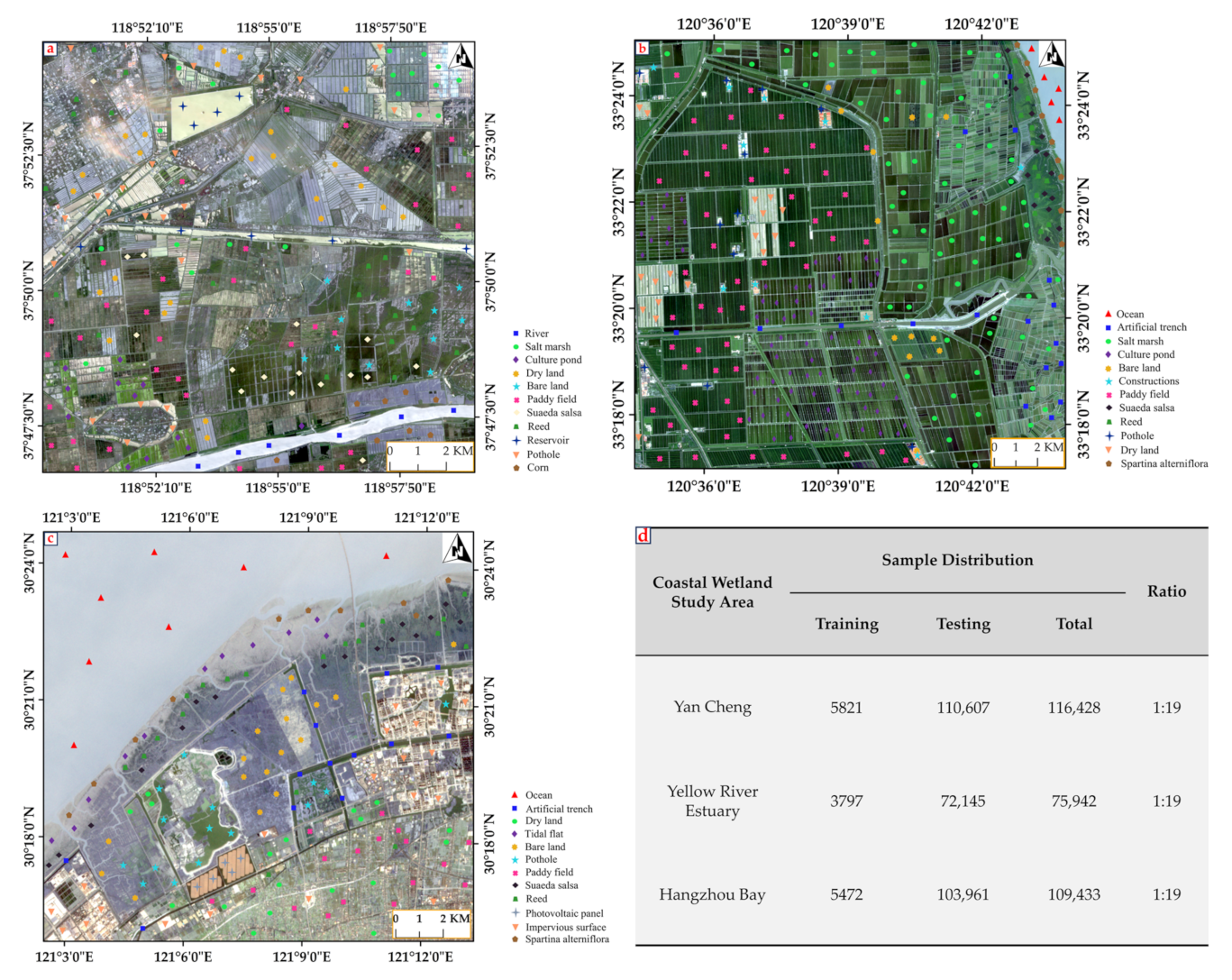
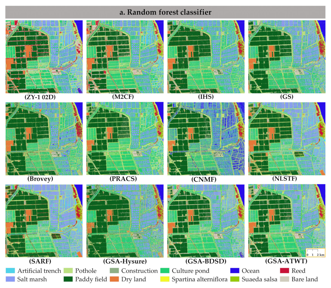
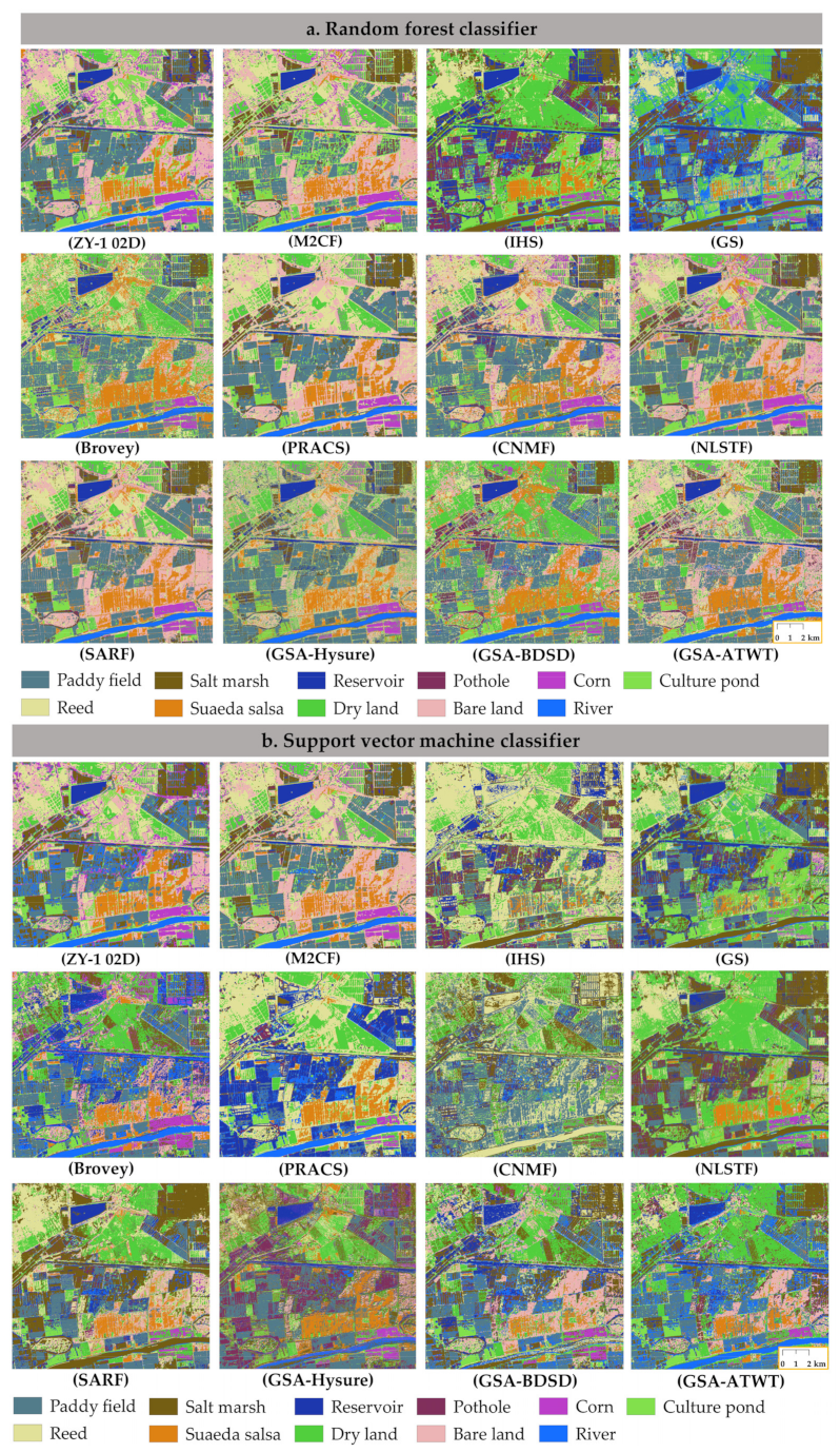
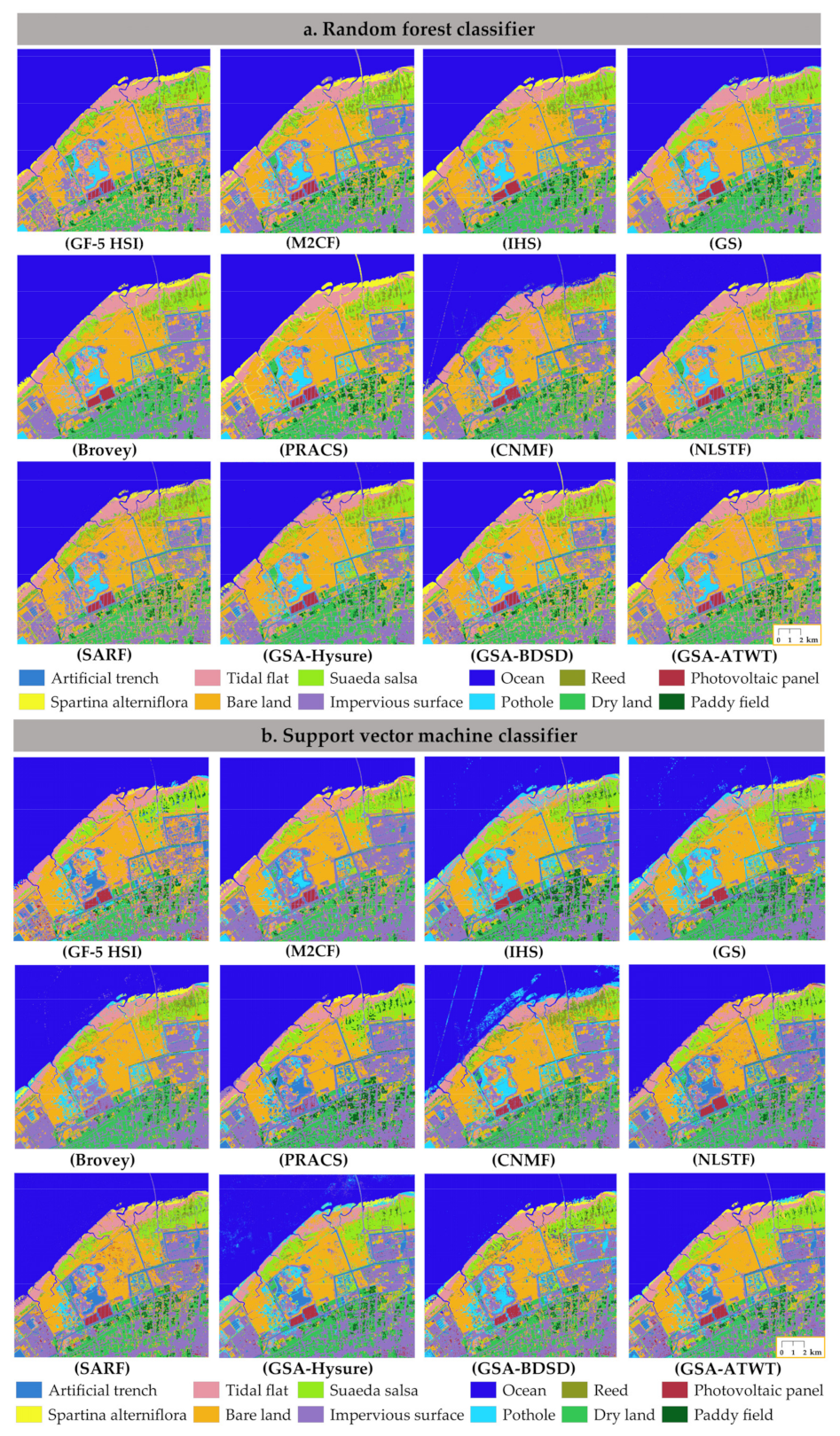
This research will fill a gap that focuses on developing a cross-modal, fast, and robust fusion method of the HS, MS, and SAR images for coastal wetlands mapping. The experiments confirm that the classification accuracy of cross-modal fusion images mostly exceeds those based on single HS or optical fusion (MS and HS) images. It is consistent with many fusion studies; that is, the appropriate fusion algorithm can improve the classification accuracy [17,20,45,56]. Besides the results presented in the experiments, the following points should be further explored. The CS fusion frameworks have advantages in high efficiency and spatial enhancement. This is the reason why CS-based methods are most widely used in SAR and optical image fusion. Hyperspectral super-resolution or unmixing-based methods are better compared to CS-based methods, but they have poor performance in cross-modal data. Hybrid methods are an available fusion option. Multi-resolution analysis can strike a balance between spectral fidelity and spatial enhancement. It avoids instability due to the uncertainty of a step-by-step framework. Among the experimental results, the proposed M2CF achieves the smallest spectral loss while obtaining the highest classification accuracy. Unfortunately, M2CF may not be suitable for fusion at large spatial resolution ratios or mountainous topography. It is mainly limited to radar shadows caused by foreshortening and layover. Joint classification using cross-modal RS data fusion for wetlands mapping is promising [2,14,16,30]. Recent trends suggest that research in cross-modal fusion is progressing towards deep learning [57]. Because of the nonlinear correlation and inherent uncertainties in data sources, the above fusion results may not be as excellent as iteratively optimized deep learning algorithms.

Taking Yancheng as an example,

Table 9. Ablation experiment of Yancheng.

Fusion Methods	Quantitative Metrics					Running Time
	PSNR	SAM	CC	RMSE	ERGAS
Low-pass Filter	29.4262	3.9817	0.81032	0.01518	17.3140	268.9314
Gaussian Filter	33.9373	3.2910	0.96010	0.01380	12.1189	319.6040
Uncompensated	23.5187	8.9363	0.76335	0.04641	35.1931	283.6111
M2CF (Proposed)	38.1668	2.5525	0.9938	0.01150	7.0877	355.8300

reports more cases as the supplement to the ablation experiment of M2CF in Yancheng. As a multi-frequency extraction experiment, Gaussian and Low-pass filters are incorporated into the method ablation. M2CF is based on MRA models, while M2CF is composed of edge-preserving filters. It is observed that the SAM and RMSE of the proposed module will increase significantly when using Gaussian and Low-pass filters to extract multi-frequency information. Specifically, the spectral metrics of the fusion module are more distorted without the spectral compensation; it further illustrates that the components work better together.

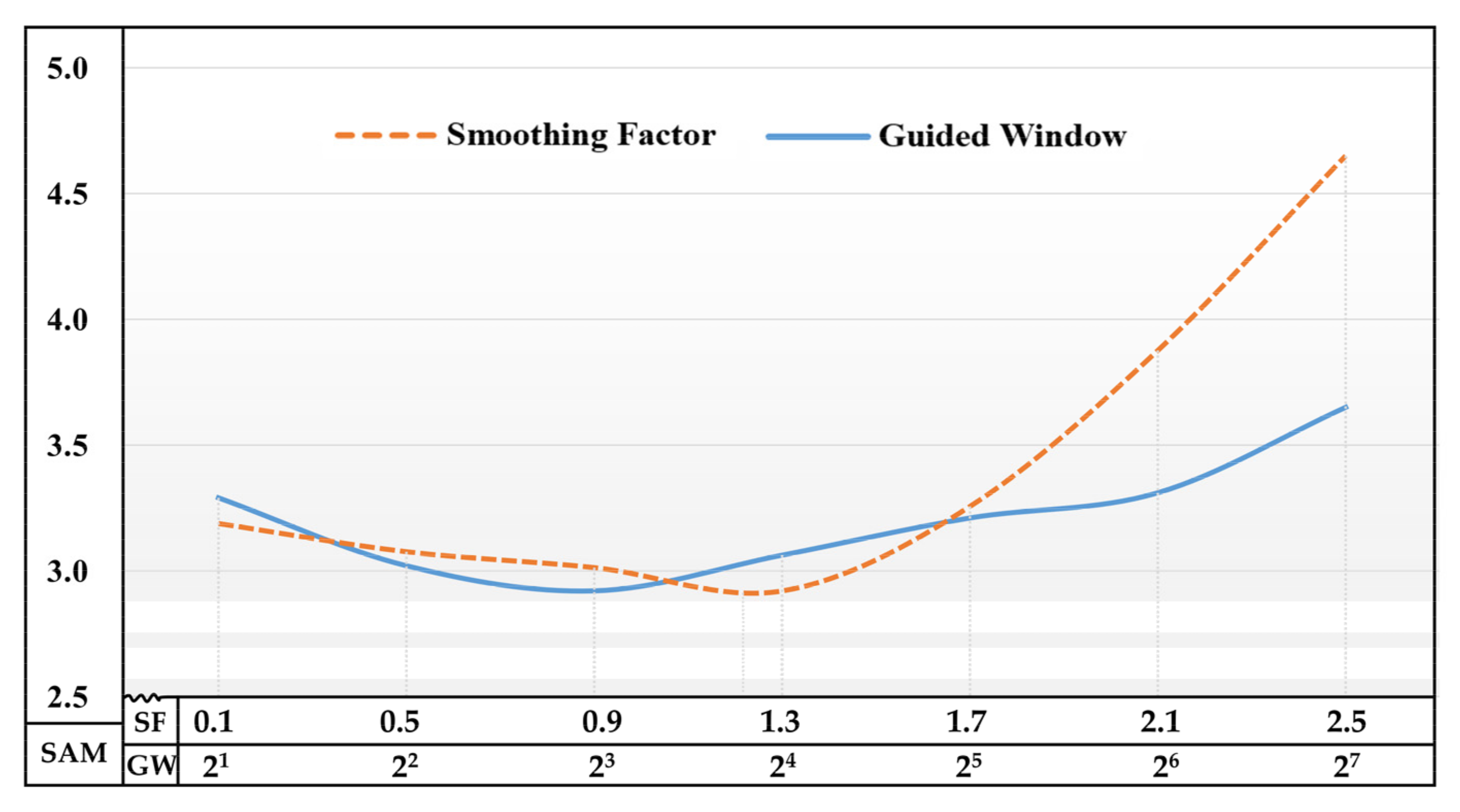
In this work, two filter parameters need to be set manually, namely the smoothing factor λ of Equation (2) and the guiding window ω of Equation (15). We applied controlled variable experiments to verify the sensitivity of the parameters. The factor of the WlsF smoothing term depends on the input image. When the gradient of the input image is relatively large, we want the constraint to be smaller to preserve the structural information of the image; when the gradient of the image is small, this detailed information is considered unimportant, and the constraint can naturally be larger. For the guided filter, each pixel is contained in multiple filter windows, and the window size is directly related to the edge-preserving of the output image. Figure 11 shows the correlation between SAM and parameter settings. For the experiment process, the guide window (GW) is 8, and the smoothing factor (SF) is 1.2, separately.

In addition, current studies often lack ground-truth and benchmark datasets at larger spatial scales. Variations in spatial registration and radiation mismatch between the SAR and optical are also major challenges. Periodic tide levels make remote sensing of coastal wetlands still challenging, which also increases the variability of data fusion [58]. Therefore, progress in this field still requires improvements in more robust fusion techniques and systematic procedures to assess the benefits of fusion.

6. Conclusions

In this paper, a hyperspectral–multispectral–SAR image fusion algorithm, namely multi-modal MRA collaborative fusion (M2CF), is offered. The proposed model improves generalized MRA and allows homogeneous data to be simultaneously integrated with physically heterogeneous radar radiation. It not only utilizes spectral–spatial information of the optical images, but also injects geometric and polarimetric properties of SAR. Fusion yields steady visible benefits, achieving the minimum spectral loss with high PSNR. Compared to step-by-step fusion frameworks, M2CF is more adjustable and robust. The classification experiments also illustrate that M2CF fused images bring about +3.2% OA improvements compared to optical fused images. Finally, we discuss two parameter settings and the ablation experiment for reference. Optical and SAR image fusion still has great potential; in the future, we will develop fusion algorithms using deep learning or feature learning.

References

1. Chang, M.; Meng, X.; Sun, W.; Yang, G.; Peng, J. Collaborative Coupled Hyperspectral Unmixing Based Subpixel Change Detection for Analyzing Coastal Wetlands. IEEE J. Sel. Top. Appl. Earth Obs. Remote Sens. 2021, 14, 8208–8224. [Google Scholar] [CrossRef]
2. Kulkarni, S.C.; Rege, P.P. Pixel level fusion techniques for SAR and optical images: A review. Inf. Fusion 2020, 59, 13–29. [Google Scholar] [CrossRef]
3. Chandrakanth, R.; Saibaba, J.; Varadan, G.; Raj, P.A. Feasibility of high resolution SAR and multispectral data fusion. In Proceedings of the 2011 IEEE International Geoscience and Remote Sensing Symposium (IGARSS), Vancouver, BC, Canada, 24–29 July 2011; pp. 356–359. [Google Scholar]
4. Mahdianpari, M.; Salehi, B.; Mohammadimanesh, F.; Brisco, B.; Homayouni, S.; Gill, E.; DeLancey, E.R.; Bourgeau-Chavez, L. Big data for a big country: The first generation of Canadian wetland inventory map at a spatial resolution of 10-m using Sentinel-1 and Sentinel-2 data on the Google Earth Engine cloud computing platform. Can. J. Remote Sens. 2020, 46, 15–33. [Google Scholar] [CrossRef]
5. Yokoya, N.; Grohnfeldt, C.; Chanussot, J. Hyperspectral and multispectral data fusion: A comparative review of the recent literature. IEEE Geosci. Remote Sens. Mag. 2017, 5, 29–56. [Google Scholar] [CrossRef]
6. Meng, X.; Shen, H.; Yuan, Q.; Li, H.; Zhang, L.; Sun, W. Pansharpening for cloud-contaminated very high-resolution remote sensing images. IEEE Trans. Geosci. Remote Sens. 2018, 57, 2840–2854. [Google Scholar] [CrossRef]
7. Drusch, M.; Del Bello, U.; Carlier, S.; Colin, O.; Fernandez, V.; Gascon, F.; Hoersch, B.; Isola, C.; Laberinti, P.; Martimort, P. Sentinel-2: ESA’s optical high-resolution mission for GMES operational services. Remote Sens. Environ. 2012, 120, 25–36. [Google Scholar] [CrossRef]
8. Ren, K.; Sun, W.; Meng, X.; Yang, G.; Du, Q. Fusing China GF-5 Hyperspectral Data with GF-1, GF-2 and Sentinel-2A Multispectral Data: Which Methods Should Be Used? Remote Sens. 2020, 12, 882. [Google Scholar] [CrossRef] [Green Version]
9. Mleczko, M.; Mróz, M. Wetland mapping using sar data from the sentinel-1a and tandem-x missions: A comparative study in the biebrza floodplain (Poland). Remote Sens. 2018, 10, 78. [Google Scholar] [CrossRef] [Green Version]
10. Moreira, A.; Prats-Iraola, P.; Younis, M.; Krieger, G.; Hajnsek, I.; Papathanassiou, K.P. A tutorial on synthetic aperture radar. IEEE Geosci. Remote Sens. Mag. 2013, 1, 6–43. [Google Scholar] [CrossRef] [Green Version]
11. Ackermann, N.; Thiel, C.; Borgeaud, M.; Schmullius, C. Potential of fusion of SAR and optical satellite imagery for biomass estimation in temperate forested areas. In Proceedings of the Proc. of the ESA Living Planet Symp, Bergen, Norway, 28 June–2 July 2010; p. 43. [Google Scholar]
12. Schmitt, A.; Leichtle, T.; Huber, M.; Roth, A. On the use of dual-co-polarized TerraSAR-X data for wetland monitoring. Int. Arch. Photogramm. Remote Sens. Spat. Inf. Sci. 2012, 39, B7. [Google Scholar] [CrossRef] [Green Version]
13. Joshi, N.; Baumann, M.; Ehammer, A.; Fensholt, R.; Grogan, K.; Hostert, P.; Jepsen, M.R.; Kuemmerle, T.; Meyfroidt, P.; Mitchard, E.T. A review of the application of optical and radar remote sensing data fusion to land use mapping and monitoring. Remote Sens. 2016, 8, 70. [Google Scholar] [CrossRef] [Green Version]
14. Lin, K.; Li, W.; Liu, H.; Wu, J. Different Levels Multi-source Remote Sensing Image Fusion. In Proceedings of the 2019 IEEE International Conference on Signal, Information and Data Processing (ICSIDP), Chongqing, China, 11–13 December 2019; pp. 1–5. [Google Scholar]
15. Pereira, L.d.O.; Freitas, C.d.C.; Sant´ Anna, S.J.S.; Lu, D.; Moran, E.F. Optical and radar data integration for land use and land cover mapping in the Brazilian Amazon. GISci. Remote Sens. 2013, 50, 301–321. [Google Scholar] [CrossRef]
16. Mahyoub, S.; Fadil, A.; Mansour, E.; Rhinane, H.; Al-Nahmi, F. Fusing of optical and synthetic aperture radar (SAR) remote sensing data: A systematic literature review (SLR). Int. Arch. Photogramm. Remote Sens. Spat. Inf. Sci. 2019, 42, 127–138. [Google Scholar] [CrossRef] [Green Version]
17. Wu, W.; Guo, S.; Cheng, Q. Fusing optical and synthetic aperture radar images based on shearlet transform to improve urban impervious surface extraction. J. Appl. Remote Sens. 2020, 14, 024506. [Google Scholar] [CrossRef]
18. Yin, N.; Jiang, Q. Feasibility of multispectral and synthetic aperture radar image fusion. In Proceedings of the 2013 6th International Congress on Image and Signal Processing (CISP), Hangzhou, China, 16–18 December 2013; pp. 835–839. [Google Scholar]
19. Gaetano, R.; Cozzolino, D.; D’Amiano, L.; Verdoliva, L.; Poggi, G. Fusion of SAR-optical data for land cover monitoring. In Proceedings of the 2017 IEEE International Geoscience and Remote Sensing Symposium (IGARSS), Fort Worth, TX, USA, 23–28 July 2017; pp. 5470–5473. [Google Scholar]
20. Shao, Z.; Wu, W.; Guo, S. IHS-GTF: A fusion method for optical and synthetic aperture radar data. Remote Sens. 2020, 12, 2796. [Google Scholar] [CrossRef]
21. Amarsaikhan, D.; Blotevogel, H.; Van Genderen, J.; Ganzorig, M.; Gantuya, R.; Nergui, B. Fusing high-resolution SAR and optical imagery for improved urban land cover study and classification. Int. J. Image Data Fusion 2010, 1, 83–97. [Google Scholar] [CrossRef]
22. Kulkarni, S.C.; Rege, P.P.; Parishwad, O. Hybrid fusion approach for synthetic aperture radar and multispectral imagery for improvement in land use land cover classification. J. Appl. Remote Sens. 2019, 13, 034516. [Google Scholar] [CrossRef]
23. Chen, S.; Zhang, R.; Su, H.; Tian, J.; Xia, J. SAR and multispectral image fusion using generalized IHS transform based on à trous wavelet and EMD decompositions. IEEE J. Sens. 2010, 10, 737–745. [Google Scholar] [CrossRef]
24. Yang, J.; Ren, G.; Ma, Y.; Fan, Y. Coastal wetland classification based on high resolution SAR and optical image fusion. In Proceedings of the 2016 IEEE International Geoscience and Remote Sensing Symposium (IGARSS), Beijing, China, 10–15 July 2016; pp. 886–889. [Google Scholar]
25. Byun, Y.; Choi, J.; Han, Y. An area-based image fusion scheme for the integration of SAR and optical satellite imagery. IEEE J. Sel. Top. Appl. Earth Obs. Remote Sens. 2013, 6, 2212–2220. [Google Scholar] [CrossRef]
26. Byun, Y. A texture-based fusion scheme to integrate high-resolution satellite SAR and optical images. Remote Sens. Lett. 2014, 5, 103–111. [Google Scholar] [CrossRef]
27. Garzelli, A. Wavelet-based fusion of optical and SAR image data over urban area. Int. Arch. Photogramm. Remote Sens. Spat. Inf. Sci. 2002, 34, 59–62. [Google Scholar]
28. Jia, Y.; Blum, R.S. Fusion method of SAR and optical images for urban object extraction. In Proceedings of the Remote Sensing and GIS Data Processing and Applications; and Innovative Multispectral Technology and Applications (MIPPR), Wuhan, China, 14 November 2007; p. 67900M. [Google Scholar]
29. Hu, J.; Hong, D.; Zhu, X.X. MIMA: MAPPER-induced manifold alignment for semi-supervised fusion of optical image and polarimetric SAR data. IEEE Trans. Geosci. Remote Sens. 2019, 57, 9025–9040. [Google Scholar] [CrossRef] [Green Version]
30. Hu, J.; Mou, L.; Schmitt, A.; Zhu, X.X. FusioNet: A two-stream convolutional neural network for urban scene classification using PolSAR and hyperspectral data. In Proceedings of the 2017 Joint Urban Remote Sensing Event (JURSE), Dubai, United Arab Emirates, 6–8 March 2017; pp. 1–4. [Google Scholar]
31. Li, T.; Zhang, J.; Zhao, H.; Shi, C. Classification-oriented hyperspectral and PolSAR images synergic processing. In Proceedings of the 2013 IEEE International Geoscience and Remote Sensing Symposium (IGARSS), Melbourne, Australia, 21–26 July 2013; pp. 1035–1038. [Google Scholar]
32. Koch, B. Status and future of laser scanning, synthetic aperture radar and hyperspectral remote sensing data for forest biomass assessment. ISPRS J. Photogram. Remote Sens. 2010, 65, 581–590. [Google Scholar] [CrossRef]
33. Chen, C.M.; Hepner, G.; Forster, R. Fusion of hyperspectral and radar data using the IHS transformation to enhance urban surface features. ISPRS J. Photogram. Remote Sens. 2003, 58, 19–30. [Google Scholar] [CrossRef]
34. Nasrabadi, N.M. A nonlinear kernel-based joint fusion/detection of anomalies using hyperspectral and SAR imagery. In Proceedings of the 2008 15th IEEE International Conference on Image Processing (ICIP), San Diego, CA, USA, 12–15 October 2008; pp. 1864–1867. [Google Scholar]
35. Dabbiru, L.; Samiappan, S.; Nobrega, R.A.; Aanstoos, J.A.; Younan, N.H.; Moorhead, R.J. Fusion of synthetic aperture radar and hyperspectral imagery to detect impacts of oil spill in Gulf of Mexico. In Proceedings of the 2015 IEEE international geoscience and remote sensing symposium (IGARSS), Milan, Italy, 26–31 July 2015; pp. 1901–1904. [Google Scholar]
36. Vivone, G.; Alparone, L.; Chanussot, J.; Dalla Mura, M.; Garzelli, A.; Licciardi, G.A.; Restaino, R.; Wald, L. A critical comparison among pansharpening algorithms. IEEE Trans. Geosci. Remote Sens. 2014, 53, 2565–2586. [Google Scholar] [CrossRef]
37. Meng, X.; Shen, H.; Li, H.; Zhang, L.; Fu, R. Review of the pansharpening methods for remote sensing images based on the idea of meta-analysis: Practical discussion and challenges. Inf. Fusion 2019, 46, 102–113. [Google Scholar] [CrossRef]
38. Sun, W.; Ren, K.; Meng, X.; Xiao, C.; Yang, G.; Peng, J. A band divide-and-conquer multispectral and hyperspectral image fusion method. IEEE Trans. Geosci. Remote Sens. 2021, 60, 1–13. [Google Scholar] [CrossRef]
39. Liu, J. Smoothing filter-based intensity modulation: A spectral preserve image fusion technique for improving spatial details. Int. J. Remote Sens. 2000, 21, 3461–3472. [Google Scholar] [CrossRef]
40. Zhouping, Y. Fusion algorithm of optical images and SAR with SVT and sparse representation. Int. J. Smart Sen. Intell. Syst. 2015, 8, 1123–1142. [Google Scholar] [CrossRef] [Green Version]
41. Farbman, Z.; Fattal, R.; Lischinski, D.; Szeliski, R. Edge-preserving decompositions for multi-scale tone and detail manipulation. ACM Trans. Graph. (TOG) 2008, 27, 1–10. [Google Scholar] [CrossRef]
42. He, K.; Sun, J. Fast guided filter. arXiv 2015, arXiv:1505.00996. [Google Scholar]
43. Yokoya, N.; Yairi, T.; Iwasaki, A. Coupled nonnegative matrix factorization unmixing for hyperspectral and multispectral data fusion. IEEE Trans. Geosci. Remote Sens. 2011, 50, 528–537. [Google Scholar] [CrossRef]
44. Meng, X.; Yang, G.; Shao, F.; Sun, W.; Shen, H.; Li, S. SARF: A simple, adjustable, and robust fusion method. IEEE Geosci. Remote Sens. Lett. 2021, 19, 1–5. [Google Scholar] [CrossRef]
45. Li, W.; Gao, Y.; Zhang, M.; Tao, R.; Du, Q. Asymmetric Feature Fusion Network for Hyperspectral and SAR Image Classification. IEEE Trans. Neural. Netw. Learn. Syst. 2022, 1–14. [Google Scholar] [CrossRef]
46. He, K.; Sun, W.; Yang, G.; Meng, X.; Ren, K.; Peng, J.; Du, Q. A Dual Global&Local Attention Network for Hyperspectral Band Selection. IEEE Trans. Geosci. Remote Sens. 2022, 60, 1–13. [Google Scholar]
47. Gao, Y.; Li, W.; Zhang, M.; Wang, J.; Sun, W.; Tao, R.; Du, Q. Hyperspectral and Multispectral Classification for Coastal Wetland Using Depthwise Feature Interaction Network. IEEE Trans. Geosci. Remote Sens. 2022, 60, 1–15. [Google Scholar] [CrossRef]
48. Gao, Y.; Song, X.; Li, W.; Wang, J.; He, J.; Jiang, X.; Feng, Y. Fusion Classification of HSI and MSI Using a Spatial-Spectral Vision Transformer for Wetland Biodiversity Estimation. Remote Sens. 2022, 14, 850. [Google Scholar] [CrossRef]
49. Inglada, J.; Giros, A. On the possibility of automatic multisensor image registration. IEEE Trans. Geosci. Remote Sens. 2004, 42, 2104–2120. [Google Scholar] [CrossRef]
50. Dian, R.; Li, S.; Fang, L.; Lu, T.; Bioucas-Dias, J.M. Nonlocal Sparse Tensor Factorization for Semiblind Hyperspectral and Multispectral Image Fusion. IEEE Trans. Cybern. 2019, 50, 4469–4480. [Google Scholar] [CrossRef]
51. Wald, L.; Ranchin, T.; Mangolini, M. Fusion of satellite images of different spatial resolutions: Assessing the quality of resulting images. Photogramm. Eng. Remote Sens. 1997, 63, 691–699. [Google Scholar]
52. Kahraman, S.; Bacher, R. A comprehensive review of hyperspectral data fusion with lidar and sar data. Annu. Rev. Control. 2021, 51, 236–253. [Google Scholar] [CrossRef]
53. Hong, D.; Yokoya, N.; Xia, G.-S.; Chanussot, J.; Zhu, X.X. X-ModalNet: A semi-supervised deep cross-modal network for classification of remote sensing data. ISPRS J. Photogram. Remote Sens. 2020, 167, 12–23. [Google Scholar] [CrossRef]
54. Hong, D.; Yokoya, N.; Ge, N.; Chanussot, J.; Zhu, X.X. Learnable manifold alignment (LeMA): A semi-supervised cross-modality learning framework for land cover and land use classification. ISPRS J. Photogram. Remote Sens. 2019, 147, 193–205. [Google Scholar] [CrossRef] [PubMed]
55. Jin, H.; Mountrakis, G. Fusion of optical, radar and waveform LiDAR observations for land cover classification. ISPRS J. Photogram. Remote Sens. 2022, 187, 171–190. [Google Scholar] [CrossRef]
56. Hu, J.; Hong, D.; Wang, Y.; Zhu, X.X. A comparative review of manifold learning techniques for hyperspectral and polarimetric sar image fusion. Remote Sens. 2019, 11, 681. [Google Scholar] [CrossRef] [Green Version]
57. Hong, D.; Gao, L.; Yokoya, N.; Yao, J.; Chanussot, J.; Du, Q.; Zhang, B. More diverse means better: Multimodal deep learning meets remote-sensing imagery classification. IEEE Trans. Geosci. Remote Sens. 2020, 59, 4340–4354. [Google Scholar] [CrossRef]
58. Zhang, Z.; Xu, N.; Li, Y.; Li, Y. Sub-continental-scale mapping of tidal wetland composition for East Asia: A novel algorithm integrating satellite tide-level and phenological features. Remote Sens. Environ. 2022, 269, 112799. [Google Scholar] [CrossRef]
Figure 1. Flowchart of the proposed method.
Remotesensing 14 03492 g001
Figure 2. Coastal wetlands study area. (a) Yellow River Estuary; (b) Yancheng; (c) Hangzhou Bay.
Remotesensing 14 03492 g002
Figure 3. Sample distribution and proportion. (a) Yancheng; (b) Yellow River Estuary; (c) Hangzhou Bay; (d) Sample proportion.
Remotesensing 14 03492 g003
Figure 4. Original and fusion images of Yancheng. (a) ZY-1 02D HSI. (b) Sentinel-2A MSI. (c) Sentinel-1A SAR. (d) Proposed M2CF. (e) IHS. (f) GS. (g) Brovey. (h) PRACS. (i) CNMF. (j) NLSTF. (k) SARF. (l) GSA-Hysure. (m) GSA-BDSD. (n) GSA-ATWT.
Remotesensing 14 03492 g004
Figure 5. Original and fusion images of Yellow River Estuary. (a) ZY-1 02D HSI. (b) Sentinel-2A MSI. (c) Sentinel-1A SAR. (d) Proposed M2CF. (e) IHS. (f) GS. (g) Brovey. (h) PRACS. (i) CNMF. (j) NLSTF. (k) SARF. (l) GSA-Hysure. (m) GSA-BDSD. (n) GSA-ATWT.
Remotesensing 14 03492 g005
Figure 6. Original and fusion images of Hangzhou Bay. (a) GF-5B AHSI. (b) GF-5B VIMI. (c) Sentinel-1A SAR. (d) Proposed M2CF. (e) IHS. (f) GS. (g) Brovey. (h) PRACS. (i) CNMF. (j) NLSTF. (k) SARF. (l) GSA-Hysure. (m) GSA-BDSD. (n) GSA-ATWT.
Remotesensing 14 03492 g006
Figure 7. Comparison of the spectral profiles.
Remotesensing 14 03492 g007
Figure 8. The Classification results of Yancheng. (a) RF-classifier; (b) SVM-classifier.
Remotesensing 14 03492 g008aRemotesensing 14 03492 g008b
Figure 9. The Classification results of Yellow River Estuary. (a) RF-classifier; (b) SVM-classifier.
Remotesensing 14 03492 g009
Figure 10. The Classification results of Hangzhou Bay. (a) RF-classifier; (b) SVM-classifier.
Remotesensing 14 03492 g010
Figure 11. Effect of parameter settings on M2CF.
Remotesensing 14 03492 g011