Forest Disturbance Detection with Seasonal and Trend Model Components and Machine Learning Algorithms

Abstract

Forest disturbances reduce the extent of natural habitats, biodiversity, and carbon sequestered in forests. With the implementation of the international framework Reduce Emissions from Deforestation and forest Degradation (REDD+), it is important to improve the accuracy in the estimation of the extent of forest disturbances. Time series analyses, such as Breaks for Additive Season and Trend (BFAST), have been frequently used to map tropical forest disturbances with promising results. Previous studies suggest that in addition to magnitude of change, disturbance accuracy could be enhanced by using other components of BFAST that describe additional aspects of the model, such as its goodness-of-fit, NDVI seasonal variation, temporal trend, historical length of observations and data quality, as well as by using separate thresholds for distinct forest types. The objective of this study is to determine if the BFAST algorithm can benefit from using these model components in a supervised scheme to improve the accuracy to detect forest disturbance. A random forests and support vector machines algorithms were trained and verified using 238 points in three different datasets: all-forest, tropical dry forest, and temperate forest. The results show that the highest accuracy was achieved by the support vector machines algorithm using the all-forest dataset. Although the increase in accuracy of the latter model vs. a magnitude threshold model is small, i.e., 0.14% for sample-based accuracy and 0.71% for area-weighted accuracy, the standard error of the estimated total disturbed forest area was 4352.59 ha smaller, while the annual disturbance rate was also smaller by 1262.2 ha year⁻¹. The implemented approach can be useful to obtain more precise estimates in forest disturbance, as well as its associated carbon emissions.

1. Introduction

Forest disturbance has been studied extensively especially after the recognition of its important role as a source of greenhouse gas (GHG) emissions and climate change since approximately 12–20% of the global GHG anthropogenic emissions have been attributed to this process [1,2]. Forest disturbances modify forest canopy structure and biomass content and can result from deforestation and forest degradation. Deforestation usually consists of the complete removal of forest cover at a big scale, while forest degradation involves subtle changes in forest structure and canopy cover [3]. With the future projections of climate change, improving accuracy and reducing uncertainty in mapping forest disturbances is critical, since it assures accurate estimations of forest carbon and climate change modeling [4]. In this study, forest disturbance was defined as “a relatively discrete event causing a change in the physical structure of the vegetation and surface soil” [5]. We focus on identifying disturbances that include both natural events, such as fires and anthropogenic activities—such as slash and burn agriculture and logging—that cause changes in forest structure that are detectable by remote sensing.

Remote sensing has been recognized as an important method to study forest disturbances, mapping their occurrence and quantifying their extent and severity [6,7]. Forest disturbances can be detected using different methods, each one having advantages or disadvantages depending on the dominating cause of forest disturbance. For example, disturbances caused by forest clearing for plantations (i.e., deforestation) can be estimated with relatively simple techniques such as comparing land cover maps of two different dates [8,9]. In turn, for disturbances that cause subtler changes in forests and lead to forest degradation, such as those from shifting cultivation and logging, the accurate estimation usually needs more sophisticated time series analyses and modeling such as LandTrendr or Breaks for Additive Season and Trend (BFAST) [7,10,11,12,13,14]. Regardless of the method used to detect forest disturbances, the final step usually consists of establishing a threshold to classify the disturbed and undisturbed areas [13]. There are generally two approaches to determine this threshold: expert knowledge or data-driven approach [15,16]. The first one usually implies a translation of an expert’s knowledge into a numeric threshold, while in the data-driven approach, an artificial intelligence algorithm determines the decision threshold based on a training dataset. Thus, the latter is commonly referred to as a supervised approach.

With the rapid development of artificial intelligence, the application of machine learning in remote sensing studies and particularly in change detection has become popular [17,18]. The algorithms—such as decision trees, support vector machines, artificial neural networks, random forests, among others—have been used to map land cover [19,20], detect and analyze land cover change patterns [21], and predict forest biomass [22]. For instance, Grinand et al. [20] used a random forests algorithm with a Landsat time series (2000, 2005, and 2010) to classify both land cover and deforestation in a tropical forest and obtained higher accuracy in stable land cover (84.7%) than deforestation (60.7%). Dlamini [21] predicted deforestation patterns and drivers using Bayesian classifiers and variables derived from expert knowledge including fuelwood consumption, population density, and land tenure, among others. For biomass retrieval, in situ measurements are typically associated with the corresponding spectral data from remote sensors using algorithms such as random forests, artificial neural networks, and support vector machines, among others [22].

The first step to implement a machine learning (ML) approach on time series data, usually consists of extracting different metrics that summarize important patterns in the time series, which the ML algorithms subsequently use as predictors for detecting vegetation changes or perform land-use/land-cover classifications [23,24,25]. Nowadays, several disturbance detection algorithms have included data-driven approaches in their workflows, such as Continuous Change Detection and Classification (CCDC) or Satellite Image Time Series Analysis for Earth Observation Data Cubes (SITS) with encouraging results [26,27]. However, other algorithms that have proved useful for disturbance detection, such as BFAST, have seldom been used in a data-driven approach, although the few examples that exist suggest that it could help increase its accuracy [7,28].

BFAST is a time series algorithm that fits a harmonic model to the observed data and then projects this model into the monitoring period [11,29]. Afterward, disturbances are identified as the observations that diverged from the expected model using a moving sum approach [29]. Most studies that have used BFAST for disturbance detection have relied on the use of magnitude (i.e., the difference between the observed and modeled value) to detect disturbance. However, previous studies have shown that other metrics, which we refer to as components, can be extracted as descriptors of the fitted model and when used with magnitude could enable a more accurate detection (e.g., [7,28]). Additionally, fitting separate models for different types of forest have proved useful to increase the accuracy of disturbance detection [25,30,31,32].

In Mexico, the tropical dry forest has been increasingly used for agriculture (mainly shifting cultivation), cattle raising activities and establishing human settlements, which has put pressure on local vegetation, causing not only deforestation but also degradation of the remaining forests [33,34]. As a consequence, the extent of natural habitats, biodiversity, and carbon sequestered in forests have been greatly reduced. With the implementation of the international framework Reduce Emissions from Deforestation and forest Degradation (REDD+), it is important to reduce the uncertainties in the estimation of the carbon emissions from forest disturbances [35]. Since BFAST has been shown effective in the estimation of disturbances by shifting cultivation [7,14,36], we believe the adoption of BFAST with ML algorithms can improve the quantification of forest disturbance [30].

Given the previous context, we wanted to assess the possible beneficial effect of using two different machine learning approaches on several BFAST components to identify disturbed forest areas. We focus on the following three main research questions: (1) if disturbance detection can be enhanced by using other BFAST model components, besides magnitude, under a ML approach or (2) by training separate models for each forest type (i.e., all-forest, only tropical dry forest, or only temperate forest), and (3) how random forests and support vector machines differ in their capabilities for disturbance detection.

2. Materials and Methods

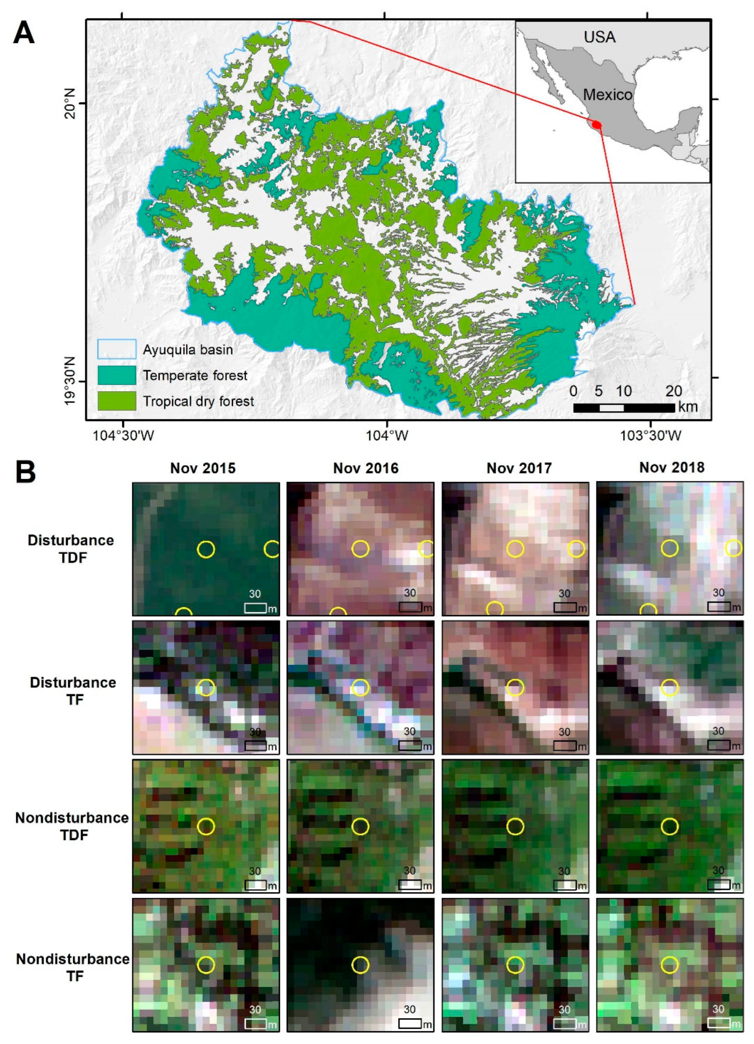
2.1. Study Site

The study area is in the Ayuquila river basin, western Mexico, with elevations ranging from approximately 250 m to 2500 m above mean sea level [37] (Figure 1). The elevation variability in the study area translates into a range of climatic conditions that include tropical semi-dry and sub-humid climates in the lower elevations, and template sub-humid and humid conditions in the higher altitudes. Annual precipitation is found in the 800–1200 mm interval and the average annual temperature is between 18 and 22 °C. The study area shows a clear rainfall seasonal pattern, where most of the precipitation falls from June to October [37].

There are two types of natural forest: temperate forest (TF) and tropical dry forest (TDF): TF covers about 12% of the watershed and is found mostly in higher elevations, while TDF occupies around 24% of the basin and is distributed usually in the lower areas. The main composition of TF includes pines (Pinus spp.), firs (Abies spp.), and oaks (Quercus spp.) and it is exploited mainly for timber, although recently, avocado (Persea americana) plantations have been established in areas previously occupied by TF. The area covered by TDF is mainly used for shifting cultivation, although residents also use TDF as natural resources for fuelwood extraction, cattle grazing, and pole extraction for constructing fences [38].

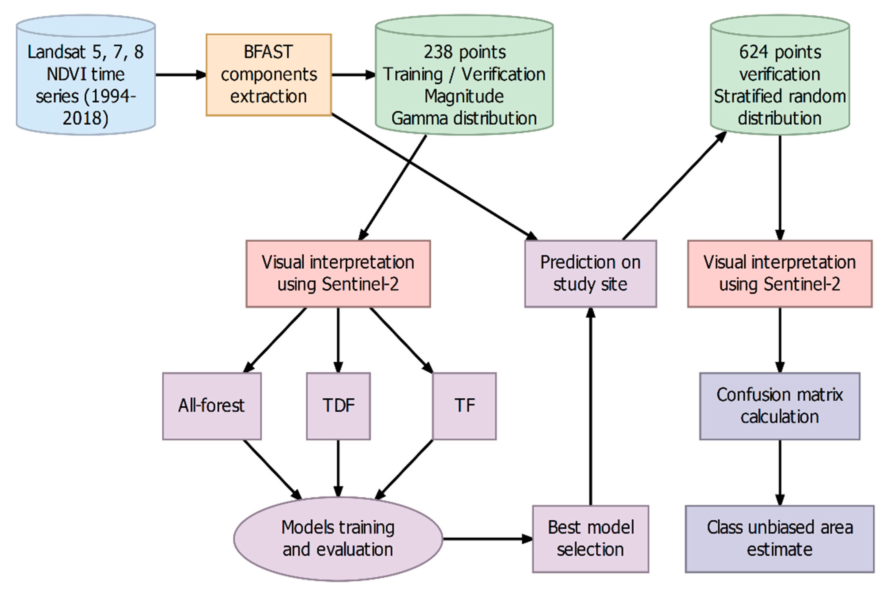
2.2. General Workflow

In a previous study, forest disturbances were identified by applying a BFAST model to an NDVI time series (1994–2018) derived from Landsat 5, 7, and 8 [30]. The time series were divided into a historical period (1994–2015) and a change monitoring period (2016–2018). We applied a threshold value of $\left|0.2\right|$ for the magnitude of change, which was derived from field verification, to optimize the detection of disturbances. Finally, we used 624 stratified random points to evaluate the detected disturbances and obtained 96.52% overall accuracy with an area-weighted error matrix [30]. These results represent the baseline model to which the ML models will be compared.

The general workflow of the methodology is presented in Figure 2. In the present study, to balance the number of observations of true and false disturbances in the training and validation datasets, we sampled 238 points based on a gamma distribution of magnitude values centered at $\left|0.2\right|$. We manually labeled those points as disturbed and non-disturbed forests using monthly median reflectance composites of Sentinel-2 images (2016–2018) as reference. Then, we trained two machine learning algorithms, random forests (RF) and support vector machines (SVM), to classify forest disturbances using the following components derived from BFAST: magnitude of change, trend, amplitude, goodness-of-fit, model fitting period, and data quality. In the following sections, we provide detailed descriptions of the methods.

2.2.1. Training and Validation Datasets

Although all the breakpoints detected by the BFAST spatial model with negative magnitude values are potential forest disturbances, those with magnitude values close to zero most probably correspond to false disturbances caused by noise or interannual variations, while those with magnitude values farther from zero will tend to correspond to true disturbances [29,39]. In order to balance the number of observations of true and false disturbances to train and validate the models, the raw magnitude output of the BFAST was used to establish a stratified random sampling design. In this procedure, we used a gamma distribution centered at magnitude $\left|0.2\right|$ to determine the number of observations for the complete range of magnitude values (0–$\left|0.5\right|$) in 0.05-value steps. A total of 238 points were selected following this design and distributed proportionally by the extent of the two types of forest. Thus, most of the visually interpreted points were close to a magnitude = $\left|0.2\right|$, while the more distant magnitude classes had fewer points (0–$\left|0.05\right|$: 10 pts, $\left|0.45\right|$–$\left|0.5\right|$: 6 pts;

Table A1. The extracted BFAST model components for the 238 training and validation data for tropical dry forest (TDF) and temperate forest (TF). The column “Change” includes disturbances, coded as 1, and non-disturbances, as 0.

Forest	Magnitude	Model Fitting Period	R2	Amplitude	Trend	Data Quality	Change
TDF	−0.0453	13.33973	0.742599	0.424708	1.84 × 10−5	96.3039	0
TDF	−0.03336	15.44384	0.784402	0.528003	1.69 × 10−5	96.9138	0
TDF	−0.0349	15.46575	0.797803	0.565893	1.75 × 10−5	96.52852	0
TDF	−0.0479	18.79452	0.769971	0.567595	2.05 × 10−5	96.18131	0
TDF	−0.03756	23.30685	0.820069	0.543106	1.09 × 10−5	96.34462	0
TDF	−0.02102	14.80822	0.628496	0.319633	2.39 × 10−5	97.00333	0
TDF	−0.00864	12.85753	0.68601	0.364489	3.27 × 10−5	96.82574	0
TDF	−0.06631	15.44384	0.697506	0.473892	2.15 × 10−5	96.64775	1
TDF	−0.05915	14.89589	0.687518	0.482008	2.30 × 10−5	96.39574	0
TDF	−0.05569	13.33973	0.738573	0.456286	2.86 × 10−5	96.22176	0
TDF	−0.05614	13.25206	0.78678	0.524416	3.29 × 10−5	96.46548	0
TDF	−0.09008	13.12055	0.802909	0.531653	3.38 × 10−5	96.59708	0
TDF	−0.07047	9.484932	0.809726	0.57334	4.58 × 10−5	95.75513	0
TDF	−0.07922	11.23836	0.747789	0.484405	5.31 × 10−5	96.29539	0
TDF	−0.06806	13.25206	0.795391	0.527232	2.91 × 10−5	96.52749	0
TDF	−0.07734	23.30685	0.824435	0.566505	1.97 × 10−5	96.37988	0
TDF	−0.05171	22.95617	0.763023	0.491165	1.58 × 10−5	96.73031	0
TDF	−0.07921	13.12055	0.751532	0.506748	3.74 × 10−5	96.51357	0
TDF	−0.09603	18.92603	0.735989	0.515702	1.73 × 10−5	96.65653	0
TDF	−0.08817	11.36986	0.741998	0.441381	3.89 × 10−5	96.21778	0
TDF	−0.10289	13.47123	0.56757	0.450491	3.20 × 10−5	96.40098	0
TDF	−0.10503	9.441096	0.743041	0.49261	5.59 × 10−5	95.88048	0
TDF	−0.13812	4.358904	0.3772	0.182208	6.35 × 10−5	94.53518	0
TDF	−0.1096	13.38356	0.699271	0.510579	4.29 × 10−5	97.89194	0
TDF	−0.11448	13.12055	0.735314	0.50283	4.16 × 10−5	96.59708	0
TDF	−0.10046	10.84384	0.696341	0.465479	4.73 × 10−5	96.46375	1
TDF	−0.10623	12.15616	0.635221	0.470523	5.27 × 10−5	96.4849	0
TDF	−0.11491	8.257534	0.668242	0.388748	9.26 × 10−5	94.95854	0
TDF	−0.11653	23.30685	0.802533	0.536494	1.30 × 10−5	95.95675	0
TDF	−0.1045	13.33973	0.752179	0.49432	2.59 × 10−5	96.52978	0
TDF	−0.11158	11.28219	0.768633	0.506031	4.18 × 10−5	95.92134	0
TDF	−0.12218	11.28219	0.775196	0.462432	4.91 × 10−5	96.04273	0
TDF	−0.11224	12.85753	0.744677	0.481245	4.12 × 10−5	96.46357	0
TDF	−0.13279	8.958904	0.719625	0.443881	6.46 × 10−5	95.38367	0
TDF	−0.12852	9.397261	0.708184	0.413003	5.80 × 10−5	96.93967	0
TDF	−0.10397	20.89589	0.745697	0.491635	2.77 × 10−5	97.129	0
TDF	−0.1244	11.89315	0.711711	0.461465	4.04 × 10−5	96.269	0
TDF	−0.11094	16.16438	0.699765	0.422634	3.46 × 10−5	96.61074	0
TDF	−0.12291	8.30137	0.639768	0.270452	5.85 × 10−5	95.31508	0
TDF	−0.12518	23.30685	0.740104	0.349312	2.01 × 10−5	96.73249	1
TDF	−0.12974	23.30685	0.74704	0.463843	9.89 × 10−6	96.4504	0
TDF	−0.11058	9.528768	0.638787	0.434527	5.24 × 10−5	96.43576	0
TDF	−0.15147	23.30685	0.746398	0.502824	1.15 × 10−5	96.63846	1
TDF	−0.18708	9.441096	0.818664	0.584014	4.80 × 10−5	95.79344	1
TDF	−0.17212	10.23014	0.697291	0.434703	5.31 × 10−5	96.76038	1
TDF	−0.17997	9.441096	0.67116	0.360017	4.48 × 10−5	95.70641	1
TDF	−0.18231	10.84384	0.750788	0.480562	4.91 × 10−5	96.26168	0
TDF	−0.15695	6.331507	0.587813	0.265593	0.000104	95.02596	0
TDF	−0.17338	2.213699	0.457311	0.253858	9.94 × 10−5	91.22373	0
TDF	−0.16738	18.70685	0.817585	0.562854	2.83 × 10−5	96.11949	1
TDF	−0.15555	13.38356	0.796706	0.574832	2.33 × 10−5	96.33647	1
TDF	−0.16485	11.84931	0.819431	0.542392	4.09 × 10−5	96.37078	0
TDF	−0.15863	13.23014	0.613797	0.435501	3.96 × 10−5	98.07453	0
TDF	−0.1543	14.43562	0.591812	0.397466	3.81 × 10−5	97.3055	0
TDF	−0.15364	6.2	0.635558	0.288652	8.94 × 10−5	94.92049	0
TDF	−0.15916	9.00274	0.781614	0.421343	8.11 × 10−5	95.6191	0
TDF	−0.16295	13.25206	0.669782	0.363889	4.88 × 10−5	96.09343	0
TDF	−0.17784	8.082191	0.806799	0.411957	0.000107	95.73026	0
TDF	−0.15906	2.213699	0.602617	0.329651	8.89 × 10−5	91.96539	0
TDF	−0.15487	13.25206	0.681363	0.456178	3.65 × 10−5	96.5895	0
TDF	−0.18407	15.44384	0.704641	0.455582	2.65 × 10−5	96.80738	1
TDF	−0.18126	8.30137	0.669672	0.383595	7.59 × 10−5	95.24909	0
TDF	−0.15282	9.441096	0.748614	0.464724	6.52 × 10−5	96.51871	0
TDF	−0.15459	8.213698	0.678228	0.373325	8.90 × 10−5	95.23174	0
TDF	−0.154	13.38356	0.772406	0.491027	2.40 × 10−5	96.6844	0
TDF	−0.15438	8.213698	0.7376	0.370441	8.89 × 10−5	95.4985	0
TDF	−0.16954	8.257534	0.697736	0.344804	4.68 × 10−5	95.42288	1
TDF	−0.15948	2.126027	0.394608	0.193095	9.77 × 10−5	92.02059	0
TDF	−0.2016	4.972603	0.537538	0.237246	7.83 × 10−5	94.43832	0
TDF	−0.21545	14.39178	0.702173	0.422295	3.38 × 10−5	96.00304	0
TDF	−0.20137	9.309589	0.771202	0.497091	6.13 × 10−5	96.08708	0
TDF	−0.21943	9.00274	0.725147	0.461319	4.80 × 10−5	95.71037	0
TDF	−0.23151	9.221918	0.387895	0.180028	9.39 × 10−5	95.78259	0
TDF	−0.21745	15.46575	0.756869	0.484993	3.41 × 10−5	95.90861	1
TDF	−0.21089	2.126027	0.396737	0.251341	0.000136	92.79279	1
TDF	−0.21431	12.76986	0.736191	0.47357	3.91 × 10−5	96.46075	1
TDF	−0.21274	12.15616	0.712597	0.379622	2.98 × 10−5	96.03425	1
TDF	−0.22979	13.33973	0.737281	0.510973	3.07 × 10−5	96.83778	1
TDF	−0.20081	13.47123	0.748393	0.500066	2.53 × 10−5	96.52298	0
TDF	−0.21194	9.221918	0.575599	0.391682	6.96 × 10−5	95.6935	0
TDF	−0.2365	2.038356	0.417297	0.112016	0.000314	91.81208	0
TDF	−0.21285	9.221918	0.820589	0.548374	5.06 × 10−5	95.7529	1
TDF	−0.24967	12.06849	0.746606	0.480799	5.48 × 10−5	96.09623	1
TDF	−0.22409	4.358904	0.507792	0.25495	0.000128	94.47236	0
TDF	−0.22582	9.00274	0.776578	0.513665	7.33 × 10−5	96.0146	1
TDF	−0.26288	13.38356	0.740385	0.447047	2.50 × 10−5	96.72533	1
TDF	−0.25233	7.690411	0.781609	0.3282	8.94 × 10−5	95.37037	1
TDF	−0.26758	1.20548	0.173027	0.127181	0.000184	93.19728	0
TDF	−0.2557	13.12055	0.69426	0.402674	1.98 × 10−5	96.34656	1
TDF	−0.29151	15.46575	0.713207	0.318498	3.80 × 10−5	96.79419	1
TDF	−0.25723	4.972603	0.596336	0.324313	4.65 × 10−5	94.65859	1
TDF	−0.25124	9.353425	0.70172	0.372796	5.92 × 10−5	96.07613	1
TDF	−0.2522	23.30685	0.777187	0.475274	2.21 × 10−5	95.90973	1
TDF	−0.25617	13.33973	0.613308	0.377054	2.39 × 10−5	96.44764	1
TDF	−0.2642	19.32055	0.77771	0.49598	2.09 × 10−5	96.3278	1
TDF	−0.25994	5.016438	0.537049	0.279299	0.000112	94.65066	1
TDF	−0.28576	11.28219	0.641284	0.407793	5.45 × 10−5	95.82423	1
TDF	−0.25507	7.778082	0.69847	0.328702	0.000112	95.38732	0
TDF	−0.26736	1.928767	0.430775	0.10271	0.000274	92.05674	0
TDF	−0.26181	4.79726	0.345256	0.230716	7.42 × 10−5	95.26256	0
TDF	−0.27483	14.28219	0.669939	0.494723	3.56 × 10−5	97.81358	0
TDF	−0.31231	13.25206	0.64658	0.30675	4.80 × 10−5	96.89954	1
TDF	−0.3047	9.484932	0.645115	0.420937	6.90 × 10−5	95.69737	1
TDF	−0.34894	5.936986	0.745417	0.151747	0.000195	94.97233	0
TDF	−0.30696	4.819178	0.545039	0.258097	8.34 × 10−5	94.375	1
TDF	−0.33039	4.928767	0.478812	0.290819	0.000117	95.22222	1
TDF	−0.32061	5.10411	0.606013	0.162013	0.000169	95.49356	0
TDF	−0.33084	1.972603	0.444768	0.096748	0.000329	92.23301	0
TDF	−0.31088	2.016438	0.460919	0.17107	0.000253	91.72321	0
TDF	−0.31157	3.221918	0.329094	0.305707	5.59 × 10−5	93.71283	1
TDF	−0.34317	4.819178	0.495519	0.113864	0.000169	94.65909	0
TDF	−0.38357	19.93151	0.812695	0.263614	4.40 × 10−5	96.1105	1
TDF	−0.35445	1.315068	0.093447	0.086669	0.000251	93.34719	0
TDF	−0.35312	14.72055	0.274482	0.248357	3.63 × 10−5	99.33011	0
TDF	−0.36574	9.309589	0.658602	0.392694	7.94 × 10−5	95.61636	1
TDF	−0.38864	23.30685	0.679754	0.328225	1.58 × 10−5	96.28585	1
TDF	−0.37412	23.30685	0.62383	0.253992	2.19 × 10−5	96.23883	1
TDF	−0.35913	5.542466	0.530187	0.193277	0.000159	95.65218	0
TDF	−0.36352	2.191781	0.681885	0.131829	0.000522	93.13358	0
TDF	−0.35709	9.441096	0.691955	0.296064	6.17 × 10−5	95.70641	1
TDF	−0.36066	4.753425	0.613245	0.417467	4.41 × 10−6	94.93088	1
TDF	−0.35418	8.345205	0.670651	0.391838	8.52 × 10−5	95.43813	1
TDF	−0.35952	5.871233	0.481878	0.14312	0.000147	95.89552	0
TDF	−0.35333	5.10411	0.572429	0.185931	0.000162	95.27897	0
TDF	−0.43061	5.060274	0.541295	0.088574	0.000207	95.34632	0
TDF	−0.40675	4.79726	0.414465	0.292673	0.000112	94.92009	1
TDF	−0.4392	3.964384	0.625067	0.101401	0.000212	94.40607	0
TDF	−0.41748	4.819178	0.426473	0.291789	0.00012	94.77273	1
TDF	−0.43424	4.753425	0.674289	0.134221	0.000208	94.87327	0
TDF	−0.40256	1.643836	0.396256	0.261978	0.000442	92.34609	0
TDF	−0.42082	5.016438	0.543248	0.077793	0.000196	95.19651	0
TDF	−0.41716	19.05754	0.855686	0.288564	5.29 × 10−5	96.11902	1
TDF	−0.40572	5.542466	0.781963	0.129629	0.000244	94.96047	0
TDF	−0.46477	1.249315	0.323113	0.127325	0.000484	92.77899	0
TDF	−0.48301	13.38356	0.591082	0.190154	2.10 × 10−5	96.47974	1
TDF	−0.47109	14.72055	0.600144	0.21734	1.68 × 10−5	96.57611	1
TDF	−0.49806	1.249315	0.283891	0.108266	0.000501	93.21663	0
TF	−0.02262	12.94521	0.290045	0.162023	9.13 × 10−6	97.67245	0
TF	−0.04735	13.33973	0.533457	0.384551	2.15 × 10−5	96.55031	0
TF	−0.04572	18.53151	0.610069	0.435479	1.48 × 10−5	96.4819	0
TF	−0.03922	14.39178	0.459061	0.339841	2.66 × 10−5	97.0118	0
TF	−0.01476	22.95617	0.194485	0.061185	1.06 × 10−5	96.84964	0
TF	−0.09167	11.63288	0.648829	0.32088	5.35 × 10−5	97.00965	0
TF	−0.0851	17.08493	0.794337	0.541089	2.39 × 10−5	96.5368	0
TF	−0.07219	11.84931	0.719495	0.305059	2.03 × 10−5	96.67129	0
TF	−0.05056	9.309589	0.527394	0.237606	3.91 × 10−5	96.41071	0
TF	−0.05958	23.30685	0.813945	0.567206	1.74 × 10−5	95.9685	0
TF	−0.05932	11.89315	0.791564	0.491535	4.10 × 10−5	96.70659	0
TF	−0.05597	14.30411	0.700437	0.414025	3.26 × 10−5	97.35734	0
TF	−0.06039	22.95617	0.651963	0.371185	1.80 × 10−5	96.31265	0
TF	−0.05082	12.76986	0.431005	0.151947	1.39 × 10−5	97.29729	0
TF	−0.0906	11.10685	0.668254	0.311451	6.02 × 10−5	96.94205	0
TF	−0.12488	21.44384	0.45162	0.102976	1.95 × 10−5	99.66786	0
TF	−0.10756	21.4	0.737156	0.237393	1.74 × 10−5	99.66718	0
TF	−0.11522	11.89315	0.684706	0.415467	4.90 × 10−5	96.79871	0
TF	−0.10173	11.23836	0.703277	0.336983	3.85 × 10−5	95.90543	0
TF	−0.11942	13.5589	0.696524	0.445791	4.17 × 10−5	96.60606	0
TF	−0.13365	11.93699	0.732592	0.393546	4.92 × 10−5	96.71868	0
TF	−0.10699	12.98904	0.680897	0.455962	3.91 × 10−5	96.2674	0
TF	−0.12874	12.15616	0.664849	0.364463	3.99 × 10−5	96.66516	0
TF	−0.12132	12.15616	0.694252	0.444977	2.90 × 10−5	96.77782	0
TF	−0.11947	10.8	0.628612	0.407771	4.43 × 10−5	96.47476	0
TF	−0.10282	12.76986	0.725571	0.460912	3.73 × 10−5	96.50365	0
TF	−0.10412	14.28219	0.675229	0.420696	3.12 × 10−5	97.52589	0
TF	−0.1135	11.84931	0.67075	0.437291	3.66 × 10−5	96.60194	0
TF	−0.11109	8.871233	0.802405	0.473938	6.59 × 10−5	96.14079	0
TF	−0.14817	8.652055	0.618584	0.328632	6.05 × 10−5	96.5812	1
TF	−0.1203	9.353425	0.665537	0.399402	5.84 × 10−5	96.19327	0
TF	−0.17207	13.38356	0.704662	0.452327	2.81 × 10−5	96.60254	1
TF	−0.16097	9.441096	0.785223	0.545458	3.92 × 10−5	96.02553	1
TF	−0.15033	11.63288	0.632914	0.329545	4.00 × 10−5	96.77419	0
TF	−0.15738	23.30685	0.553428	0.165368	1.99 × 10−5	96.96756	0
TF	−0.1807	3.616438	0.446501	0.250369	8.97 × 10−5	95.76079	0
TF	−0.16262	11.84931	0.719112	0.470987	5.08 × 10−5	96.11651	1
TF	−0.16764	23.30685	0.682412	0.394082	1.45 × 10−5	96.25059	1
TF	−0.15789	10.58082	0.107594	0.091385	−8.90 × 10−6	97.25602	0
TF	−0.15251	14.80822	0.75305	0.477127	4.00 × 10−5	96.70736	0
TF	−0.16294	13.38356	0.725956	0.459349	2.95 × 10−5	96.54114	1
TF	−0.17463	11.84931	0.771981	0.42334	5.44 × 10−5	96.78687	0
TF	−0.17676	4.753425	0.558608	0.289002	4.29 × 10−5	95.39171	0
TF	−0.19765	17.96164	0.749915	0.492095	2.97 × 10−5	96.41605	1
TF	−0.16569	21.44384	0.620788	0.197482	2.65 × 10−5	99.62953	0
TF	−0.19886	12.85753	0.761269	0.506095	3.72 × 10−5	96.44227	0
TF	−0.17335	4.490411	0.649241	0.376716	9.77 × 10−5	98.10976	0
TF	−0.1625	4.79726	0.683543	0.332143	3.88 × 10−5	96.00457	0
TF	−0.17013	8.082191	0.754489	0.377575	7.03 × 10−5	96.34023	0
TF	−0.16837	8.345205	0.783846	0.366675	6.62 × 10−5	96.7509	0
TF	−0.21632	13.12055	0.76959	0.512075	4.15 × 10−5	96.05428	1
TF	−0.22559	23.30685	0.67785	0.289514	1.75 × 10−5	96.19182	1
TF	−0.21154	12.85753	0.766562	0.538063	5.30 × 10−5	96.48487	1
TF	−0.2329	12.98904	0.720822	0.459314	2.35 × 10−5	96.39393	1
TF	−0.20149	22.95617	0.360888	0.153679	1.54 × 10−5	96.34845	1
TF	−0.20698	15.29041	0.710478	0.461842	2.48 × 10−5	96.16625	1
TF	−0.22487	18.66301	0.737929	0.454678	3.01 × 10−5	96.46265	1
TF	−0.22928	3.090411	0.465788	0.396536	3.93 × 10−5	95.5713	0
TF	−0.20556	4.643836	0.518488	0.233282	0.000115	96.93396	0
TF	−0.24299	23.30685	0.684501	0.287483	2.18 × 10−5	96.20358	1
TF	−0.22637	15.33425	0.618501	0.349496	7.43 × 10−6	96.01643	1
TF	−0.21411	11.89315	0.633748	0.382813	5.96 × 10−5	96.91386	0
TF	−0.28623	23.30685	0.539063	0.233548	1.54 × 10−5	96.21532	1
TF	−0.25423	14.43562	0.811445	0.387543	6.03 × 10−5	96.33776	1
TF	−0.26478	4.709589	0.650802	0.40437	7.81 × 10−5	96.10465	1
TF	−0.27368	11.89315	0.760329	0.481602	5.42 × 10−5	96.79871	1
TF	−0.26242	8.082191	0.497489	0.22214	7.84 × 10−5	96.00136	0
TF	−0.25918	13.33973	0.726444	0.275718	2.65 × 10−5	96.50924	1
TF	−0.29659	23.30685	0.615274	0.209382	2.50 × 10−5	96.25059	1
TF	−0.27568	14.34795	0.598175	0.308084	8.78 × 10−6	96.37266	1
TF	−0.2631	8.871233	0.646465	0.278076	9.89 × 10−5	96.17166	0
TF	−0.27551	7.164383	0.440842	0.227169	9.23 × 10−5	95.75688	0
TF	−0.25938	7.164383	0.52456	0.260804	9.30 × 10−5	95.83334	0
TF	−0.27658	22.95617	0.665763	0.373353	1.70 × 10−5	96.46778	1
TF	−0.31804	5.958904	0.720874	0.496008	9.05 × 10−5	99.35662	0
TF	−0.30249	23.30685	0.581094	0.218389	1.65 × 10−5	96.2976	1
TF	−0.32208	23.30685	0.611473	0.238884	2.01 × 10−5	96.19182	1
TF	−0.3278	4.709589	0.52152	0.35563	8.87 × 10−5	96.10465	1
TF	−0.33703	23.30685	0.614924	0.252018	1.54 × 10−5	96.25059	1
TF	−0.33582	23.30685	0.629637	0.266593	2.00 × 10−5	96.26234	1
TF	−0.34522	4.79726	0.498216	0.230261	5.87 × 10−5	94.97717	1
TF	−0.34275	12.37534	0.751576	0.302551	4.66 × 10−5	96.28154	1
TF	−0.3581	23.30685	0.463526	0.196457	1.43 × 10−5	96.22708	1
TF	−0.36095	7.361644	0.596833	0.209501	0.000146	96.05655	0
TF	−0.36794	23.30685	0.522918	0.224043	1.50 × 10−5	96.34462	1
TF	−0.36408	12.85753	0.503183	0.289444	1.40 × 10−5	96.25053	1
TF	−0.35931	23.30685	0.592758	0.219493	1.60 × 10−5	96.27409	1
TF	−0.36242	12.94521	0.59287	0.368999	2.72 × 10−5	95.93737	1
TF	−0.37269	23.30685	0.589095	0.22655	1.72 × 10−5	96.32111	1
TF	−0.38235	11.15069	0.55248	0.184192	1.70 × 10−5	95.99607	1
TF	−0.37201	23.30685	0.553574	0.112416	2.19 × 10−5	97.03808	1
TF	−0.37854	12.33151	0.665211	0.251212	2.17 × 10−5	96.24612	1
TF	−0.41557	10.27397	0.534546	0.178508	2.16 × 10−5	96.16103	1
TF	−0.41685	23.30685	0.561889	0.199097	1.80 × 10−5	96.30936	1
TF	−0.41672	10.75616	0.560494	0.169953	2.24 × 10−5	96.15482	1
TF	−0.40322	13.33973	0.295362	0.09462	1.64 × 10−5	97.41273	1
TF	−0.43973	23.30685	0.570338	0.228854	1.47 × 10−5	96.30936	1
TF	−0.41507	23.30685	0.522161	0.207258	1.56 × 10−5	96.20358	1
TF	−0.45598	23.30685	0.560614	0.209294	1.73 × 10−5	96.32111	1
TF	−0.48716	4.79726	0.691486	0.300189	0.000124	94.97717	0
TF	−0.45247	23.30685	0.560478	0.205325	1.56 × 10−5	96.41514	1

).

These points were labeled manually as disturbed and non-disturbed. For this, we consulted Sentinel-2 images from 2016–2018 in GEE at level 1C, which were orthorectified and radiometrically calibrated. Sentinel-2 images provided by the European Space Agency (ESA) have spatial resolutions ranging from 10 m to 60 m and multi-spectral bands covering the visible, red edge, and infrared spectral range and a temporal resolution of 2–5 days [40]. We first applied a cloud mask using the data quality layer ‘QA60’ and then we constructed monthly time series images using the median value. For each image, we used blue, green, and red channels with a spatial resolution of 10 m to construct natural color composites. Using the monthly natural color composites, we visually interpreted the sample points and labeled them as either disturbed or non-disturbed forest. When the interpretation was not clear with the Sentinel-2 images, we consulted high spatial resolution images in Google Earth. Some examples of Sentinel-2 images for sample points interpretation as disturbance and non-disturbance in TDF and TF are in Figure 1B.

After visually interpreting the 238 points, 143 points corresponded to non-disturbed forest (TF: 53 and TDF: 48), while 95 points, to disturbed forest (TF: 90, TDF: 47). This distribution confirmed that the followed stratified random sample helped in obtaining a more balanced dataset in terms of the number of observations of the disturbance/non-disturbance classes. Afterward, the verified points were split at random into training and validation datasets with a proportion of 0.7/0.3, respectively. It has been reported that forest type is an important factor in classifying forest disturbance using BFAST [30,31,32], therefore, three models were constructed with different forest stratum: all-forest, only TDF, and only TF.

2.2.2. Variables: BFAST Components and Time Series Landsat Data Quality

BFAST has been successfully applied in characterizing spatial–temporal vegetation dynamics and detecting changes in a time series [7,11,36]. BFAST model focuses on near real-time change detection, by which data is divided into a historical and monitoring period. The stable trend, modeled in the historical period, is projected into the monitoring period and a breakpoint of change is detected when the difference between the projected and observed values is larger than a threshold [29]. Usually, magnitude of change is the variable that is adjusted to optimize the detection [29,39,41]. However, a range of other variables can be obtained from the BFAST model such as trend, amplitude of the seasonal model, goodness-of-fit, model fitting period, as well as data quality in the fitted model. These variables have been tested relevant for vegetation change detection. For example, Grogan et al. [31] reported that the difference in slope of the model is important in the disturbance detection of different forest types. De Vries et al. [39] found an enhanced disturbance detection when using the breakpoints along with magnitude, while Dutrieux et al. [7] and Schultz et al. [42] reported data availability as an important factor in disturbance detection.

In this work, the following BFAST model components were extracted: magnitude, trend, amplitude, goodness-of-fit, model fitting period, and data quality (

Table 1. Definition and equation of the BFAST components that were used as predictive variables in the machine learning algorithms.

Seasonal and Trend Model Components	Definition	Equation
Magnitude	The absolute value of the difference between the observed and projected NDVI	$magnitude=\left|y_{break}-{\widehat{y}}_{break}\right|$
Trend	The trend of the linear model that was fitted in the stable historical data period	$slope=\frac{n{{\displaystyle \sum }}_i\left(x_i{y}_i\right)-({{\displaystyle \sum }}_i{x}_i)({{\displaystyle \sum }}_i{y}_i)}{n({{\displaystyle \sum }}_i{x}_i^2)-{({{\displaystyle \sum }}_i{x}_i)}^2}$
Amplitude	The difference between the maximum and minimum NDVI of the detrended model	$amplitude={\widehat{y}}_{max}-{\widehat{y}}_{min}$
Goodness-of-fit	The goodness-of-fit of the fitted model measured by R2	$R^2=1-\frac{{{\displaystyle \sum }}_i{\left(y_i-{\widehat{y}}_i\right)}^2}{{{\displaystyle \sum }}_i{\left(y_i-{\overline{y}}_i\right)}^2}$
Model fitting period	The length in years of the stable historical data period, corresponding to the time window to which the BFAST model is fitted	$\begin{array}{l}history length\\ =yea{r}_{startMonitoring}\\ -yea{r}_{lastHistoricalBreak}\end{array}$
Data quality	The number of valid observations over the total observations in the stable historical data period	$data quality=\frac{n}{N}$

). The abbreviations in Table 1 are the following: i stands for each observation in a time series, $y_i$ and ${\widehat{y}}_i$ for the observed and predicted NDVI value of i, $\overline{y}$ stands for the mean NDVI, n for the number of observations in the time series, x for the independent variable (i.e., days), y stands for the dependent variable (NDVI), $y_{break}$ and ${\widehat{y}}_{break}$ for the observed and predicted value in the detected breakpoint, respectively, ${\widehat{y}}_{max}$ and ${\widehat{y}}_{min}$ for the maximum and the minimum predicted value of the detrended model, respectively, $n,$ represents valid observations and $N$ represents the total number of observations in the stable historical period, respectively. We use data quality as a measure of the percentage of valid observations over the total observations, which are 365 per year. The valid observations correspond to cloudless observations, while the total observations include valid observations, no data, cloud pixels, and missing data.

2.2.3. Baseline Model

The baseline model for forest disturbance detection uses only the threshold ($\left|0.2\right|$) of magnitude of change as a predictive variable, which was determined by field verification. With this model, an area with an absolute magnitude value higher than this threshold is classified as a disturbance. This model is applied in all three datasets with different forest stratum. The purpose of this baseline model is to have a point of comparison with the ML models using other variables of BFAST components.

2.2.4. Machine Learning Algorithm

Two ML algorithms, RF and SVM, were applied in a supervised classification scheme using variables of BFAST components and time series data quality to test if they can improve upon the baseline model. These two algorithms use non-parametric models that have been applied previously for land cover classification and change detection [18].

RF is a classification and regression algorithm based on an ensemble of multiple decision trees, trained using random samples of the data and predictor variables [43]. Predictions are designated by aggregating the estimates made by each tree using a majority vote. RF is usually trained with a proportion of two-thirds of the training data and validated by the remaining one-third, also referred to as out-of-bag dataset [43]. Previous studies have reported that using a high number of decision trees makes the generalization error converge and reduces the overfitting of the model [19,20,43]. Therefore, we use 500 random trees to perform the classification, while the number of predictive variables used in each split of each tree was the square root of the number of predictive variables. Finally, the out-of-bag ratio was one-third.

SVM is also a classification and regression algorithm that tries to find a hyperplane that minimizes the error in the predictions [44]. The hyperplane for the classification is determined by the subset of the data that fall in the decision boundary (these points are referred to as support vectors). SVM assumes that the data are linearly separable in a multidimensional space; but, since this is often not the case, kernel functions are used to transform the feature space to facilitate the classification [17]. SVM can use different types of kernel functions; however, in this study, we applied the radial basis function, which has been frequently used in remote sensing applications [45,46]. On the other hand, a key concept in SVM is the margin, which refers to the distance between the decision hyperplane and the closest observation. Usually, a large margin allows clear discrimination by the hyperplane. Thus, the cost parameter consists of a positive value indicating the penalization for predicting a sample within or on the wrong side of the margin, while the sigma is the precision parameter. In this case, we use cost = 1 and sigma was calculated automatically from the data in a heuristic procedure [47].

2.3. Variable Importance

The importance value of each predictive variable was calculated for both ML algorithms using models that included all the predictive variables. Based on the importance values, multiple models were trained sequentially, including the most important variables first. This sequential model training was applied for the three datasets: all-forest, TDF and TF. The all-forest dataset included forest-type as an additional predictor, besides the BFAST components; while the forest-type specific datasets included only the BFAST components as predictive variables. In total, seven models were trained for the all-forest dataset and six models for each of the forest-type specific datasets.

For RF models, the variable importance was calculated as a linear transformation of the Mean Decrease Gini into a 0–100 range, which measures the total decrease in node impurities resulting from splitting the data according to each predictive variable and then averaging this decrease over all the constructed trees [43]. For SVM models, the variable importance was calculated by permuting the independent variables and fitting a single-predictor model on the complete data [48]. Afterward, the predictor variable that obtained the highest value of the area under the curve (AUC) of the receiver operating characteristic (ROC) curve was ranked as 100 and the variable with the lowest AUC value as zero, while all the other importance values were scaled to this range.

2.4. Best Model Selection

To find the best model configuration in terms of the predictive variables, different models were trained using only the training dataset (n = 168), while leaving the validation data untouched (n = 70). The model training was based on a 3-fold cross-validation with 40 repeats. In this way, each model ran 120 iterations from which the average accuracy and standard error were calculated. Afterward, the best configuration was selected based on a balance between the overall accuracy and the number of variables included, such that models with fewer predictive variables and a non-significant difference with the highest achieved accuracy were prioritized (i.e., within the range of mean accuracy ± 1.96 standard error).

The identical procedure was followed in the three datasets: all-forest, TDF and TF. Although the split ratio between the training and validation datasets was the same for all the three datasets, for TDF and TF datasets, the total number of observations for each split was smaller in comparison with the all-forest dataset. In the case of TDF, training and validation datasets had 97 and 41 observations, respectively; while for TF, the same datasets had 72 and 29 observations, respectively.

The overall accuracy is defined as a metric that summarizes the number of correct predictions over the total predictions [49]. It is calculated as the ratio of the sum of the true positive and true negative cases over the total predictions as summarized in an error matrix (

Table 2. TP (true positive), FP (false positive), FN (false negative), and TN (true negative) in an error matrix for a binary classification of disturbance and non-disturbance. The ground data are located in the columns, and the predicted data are located in the rows.

	Disturbance	Non-Disturbance
Disturbance	TP	FP
Non-disturbance	FN	TN

, Equation (1)).

Overall accuracy = (TP + TN)/(TP + TN + FP + FN)

(1)

2.5. Model Validation

The trained model was tested using the validation data, which was kept untouched. Several metrics were calculated including overall accuracy, F1-score, and ROC AUC. Overall accuracy evaluates the correct detection of both disturbance and non-disturbance samples, while F1-score and ROC AUC focus on the class of interest (i.e., disturbance). Therefore, each metric evaluates a different aspect of the results.

F1-score corresponds to the harmonic mean of precision and recall, calculated as Equation (2), where p stands for precision (or user’s accuracy) and r for recall (or producer’s accuracy) [50,51]. Precision is calculated as the ratio of true positives over the total of positive predictions and recall is calculated as the ratio of the true positives over the sum of true positives and false negatives [51].

F1-score = 2 × p × r/(p + r)

(2)

The ROC curve is constructed by plotting the false positive rate against the true positive rate of a classification model, using different probability thresholds. True positive rate is a synonym for recall (see Equation (2)), while false positive is calculated as 1 − TN/(TN + FN).

ROC curves can be used to interpret the skill of a model to correctly classify a binary outcome (true or false). In our case, it shows the ability of the model to classify the disturbance class. In turn, the AUC of a ROC plot is calculated as the area under the ROC curve. For a random guess, the AUC is 0.5, while a perfect model will have an AUC of 1. Models with AUC between 0.5 and 1 represent a better prediction than a random guess, while higher AUC values are considered better models.

2.6. Post Classification Processing and Accuracy Assessment

The best model (SVM all-forest) was used to predict forest disturbance in the complete study area. Although the validation dataset was used to verify the models using an independent set of observations, this dataset was created following a gamma distribution of magnitude. Thus, it was not considered as a representative sample of the entire study area. To assess the accuracy of this classification using an independent set of validation data, a stratified random sampling was implemented based on the area occupied by each class of interest in the classification map, following [52]. The number of samples was calculated using Equation (3)

$$n=\frac{{({\sum }^{ }{W}_i{S}_i)}^2}{{[S(Ô)]}^2+\left(1/N\right){\sum }^{ }{W}_i{S}_i{}^2}\approx {(\frac{{\sum }^{ }{W}_i{S}_i}{S(Ô)})}^2,$$

(3)

where $S(Ô)$ is the standard error of the estimated overall accuracy. As suggested by Olofsson et al. [52] a value of 0.01 was used. $W_i$ is the mapped proportion of the area of class $i$ and $S_i$ is the standard deviation of class $i$, and $S_i=\sqrt{U_i\left(1-U_i\right)}$. This formula estimated a sample size of 624 observations. For the rare classes—i.e., disturbances—50 random points were assigned for each forest type. The rest of the validation points were defined according to the predicted proportional area of the remaining strata (i.e., non-disturbed forest in both TF and TDF). Afterward, these points were verified by visual interpretation in Google Earth Engine (GEE) using Sentinel-2 images.

2.7. R Packages

The complete method was carried out in an R 4.0.5 environment. Variable importance was calculated using the caret package [48], the training and validation of the ML algorithms were performed using the tidymodels [53] and yardstick packages [54], the spatial information operations were done using the sf [55] and raster packages [56], while for data wrangling and plots the tidyverse package [57] was used.

3. Results

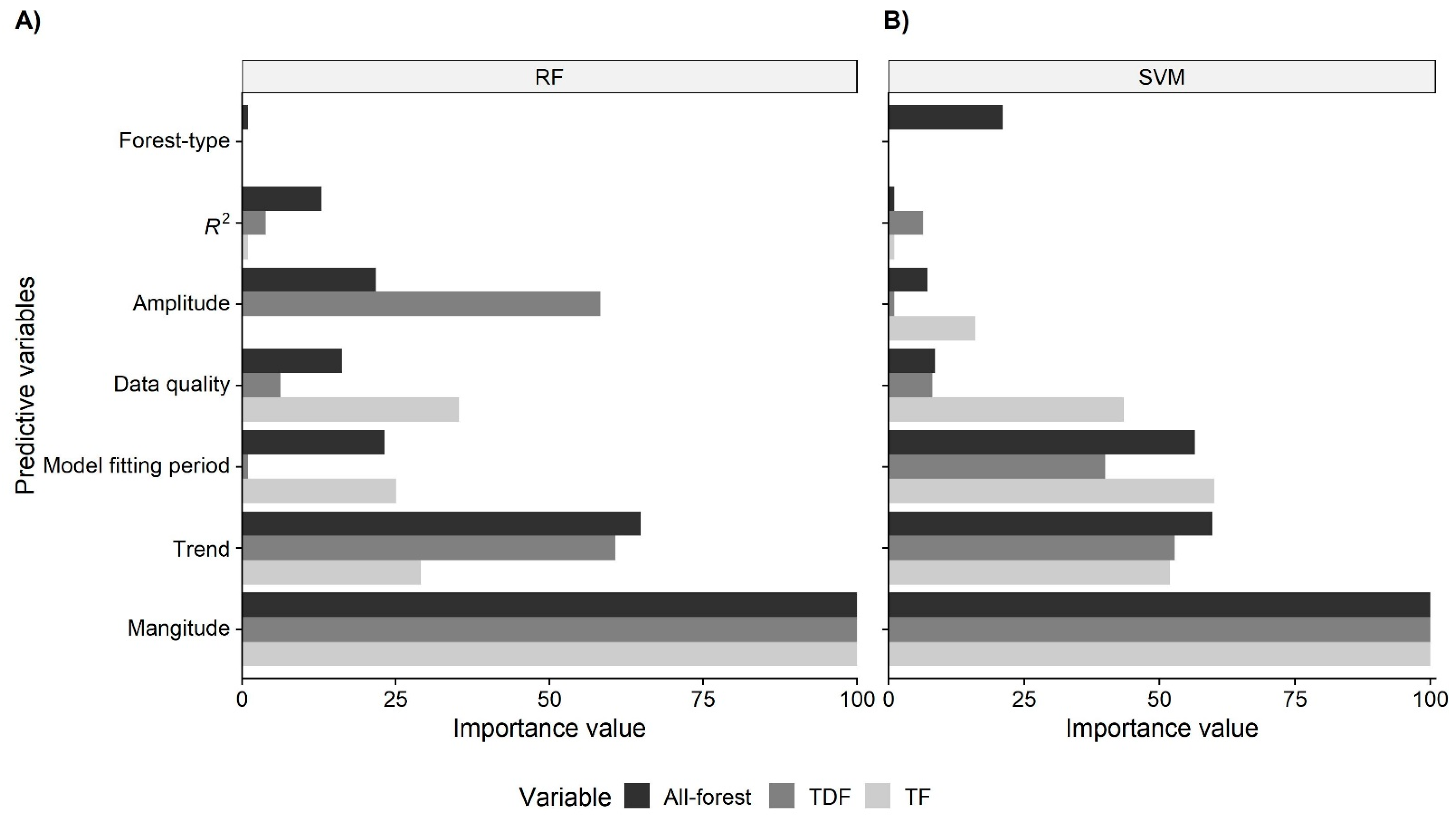
3.1. Variable Importance

The variable importance values show that the essential variables to correctly identify disturbances vary with the algorithm and dataset used (all-forest, TDF, or TF). Nevertheless, regardless of the dataset and ML algorithm, magnitude was always ranked as the most important predictor, while other important variables included trend, data quality, model fitting period, and amplitude. On the contrary, forest-type and R² were ranked as the least important (Figure 3).

3.2. Best Model Selection

The exploration of the models with a different number of predictive variables indicated that the accuracy ranged from 61.48% to 87.89% (see Figure 3 and

Table A2. Mean accuracy in range of confidence interval at 95% level obtained for each of the constructed models using the RF and SVM algorithms. The models were trained using only the random subsets of the training data (not validation data), with 120 iterations. Additionally, the models were applied in three datasets, All-forest, TDF, TF, and the variables for each dataset are indicated. The best model, marked by underlined bold font, is selected by a balance between the accuracy and the number of variables. Given similar accuracy, the models with lower number of predictive variables were preferred.

Dataset	RF		SVM
	Predictive Variables	Accuracy (%)	Predictive Variables	Accuracy (%)
All-forest	Baseline	76.78 ± 0.87	Baseline	76.78 ± 0.87
	Magnitude	70.64 ± 0.84	Magnitude	73.7 ± 0.96
	Magnitude + trend	84.15 ± 0.56	Magnitude + trend	86.45 ± 0.64
	Magnitude + trend + model fitting period	85.45 ± 0.66	Magnitude + trend + model fitting period	87.35 ± 0.59
	Magnitude + trend + model fitting period + amplitude	85.62 ± 0.68	Magnitude + trend + model fitting period + forest-type	86.02 ± 0.67
	Magnitude + trend + model fitting period + amplitude + data quality	85.87 ± 0.76	Magnitude + trend + model fitting period + forest-type + data quality	87 ± 0.61
	Magnitude + trend + model fitting period + amplitude + data quality + R2	85.52 ± 0.76	Magnitude + trend + model fitting period + forest-type + data quality + amplitude	87.89 ± 0.71
	Magnitude + trend + model fitting period + amplitude + data quality + R2 + forest-type	85.04 ± 0.8	Magnitude + trend + model fitting period + forest-type + data quality + amplitude + R2	86.56 ± 0.67
TDF	Baseline	71.04 ± 1.08	Baseline	71.04 ± 1.08
	Magnitude	61.48 ± 1.25	Magnitude	66.9 ± 1.12
	Magnitude + trend	79.17 ± 1.06	Magnitude + trend	81.93 ± 1.03
	Magnitude + trend + amplitude	80.96 ± 0.93	Magnitude + trend + model fitting period	81.9 ± 1.01
	Magnitude + trend + amplitude + data quality	81.38 ± 1	Magnitude + trend + model fittingperiod + data quality	84.22 ± 1.02
	Magnitude + trend + amplitude + data quality + R2	81.93 ± 0.93	Magnitude + trend + model fitting period+ data quality + R2	84.58 ± 0.98
	Magnitude + trend + amplitude + data quality + R2 + model fitting period	80.29 ± 1.04	Magnitude + trend + model fitting period+ data quality + R2 + amplitude	83.41 ± 1.04
TF	Baseline	84.75 ± 1.17	Baseline	84.75 ± 1.17
	Magnitude	79.46 ± 1.22	Magnitude	80.04 ± 1.15
	Magnitude + data quality	85.85 ± 1.2	Magnitude + model fitting period	85.97 ± 1.15
	Magnitude + data quality + trend	85.65 ± 1.16	Magnitude + model fitting period + trend	85.89 ± 1.07
	Magnitude + data quality + trend + model fitting period	85.28 ± 1.09	Magnitude + model fitting period + trend + data quality	86.55 ± 1.03
	Magnitude + data quality + trend + model fitting period + R2	84.82 ± 1.16	Magnitude + model fitting period + trend + data quality + R2	86.23 ± 1.1
	Magnitude + data quality + trend + model fitting period + R2 + amplitude	84.64 ± 1.18	Magnitude + model fitting period + trend + data quality + R2 + amplitude	85.43 ± 1.11

). From these results, the models that were not significantly different from the highest achieved accuracy and with less predictive variables were selected and verified on the validation set (

Table 3. Predictive variables in the best models selected by criteria of the highest accuracy and fewer predictive variables. The order of the variables indicates their importance in the model. Finally, the accuracy achieved on the validation set is shown.

Three Forest Stratum	Random Forests (RF)	Support Vector Machine (SVM)	Accuracy (%; RF vs. SVM)
All-forest	Magnitude, trend, model fitting period	Magnitude, trend, model fitting period	75.71 vs. 80.00
TDF	Magnitude, trend, amplitude	Magnitude, trend, model fitting period, data quality	80.49 vs. 75.61
TF	Magnitude, data quality	Magnitude, model fitting period	86.21 vs. 79.31

). For the all-forest model, both SVM and RF favored three identical predictive variables: magnitude, trend, and model fitting period, in the same order of importance; however, SVM obtained higher overall accuracy than RF on the validation dataset. In turn, in the RF model of TDF, the best model included magnitude, trend, and amplitude; while using SVM, it included magnitude, trend, model fitting period, and data quality. In the TF model, RF and SVM used fewer predictive variables, either magnitude and data quality for RF or magnitude and model fitting period for SVM (Table 3).

3.3. Model Validation

Regardless of the ML algorithm used, the validation of these models showed the same accuracy or an increase in accuracy of up to 21.95% compared to the baseline models (Δ Best vs. Baseline,

Table 4. Evaluation of the baseline model (with magnitude threshold = $\left|0.2\right|$) and the best models using RF and SVM on the validation dataset.

Dataset	Evaluation Metric	RF & SVM (%)	RF (%)		SVM (%)		ΔRF vs. SVM (%)
		Baseline	Best	Δ Best vs. Baseline	Best	ΔBest vs. Baseline
All-Forest	Accuracy	68.57	75.71	7.14	80.00	11.43	−4.29
	F1-score	65.63	66.67	1.04	74.07	8.45	−7.40
	ROC AUC	69.64	81.16	11.52	90.14	20.49	−8.98
Tropical Dry Forest (TDF)	Accuracy	58.54	80.49	21.95	75.61	17.07	4.88
	F1-score	51.43	69.23	17.80	54.55	3.12	14.68
	ROC AUC	59.92	88.36	28.44	79.63	19.71	8.73
Temperate Forest (TF)	Accuracy	79.31	86.21	6.90	79.31	0.00	6.90
	F1-score	81.25	86.67	5.42	78.57	2.68	8.10
	ROC AUC	79.76	90.24	10.48	91.90	12.14	−1.66

). The largest difference was observed in the TDF dataset, where the baseline model achieved an accuracy of 58.54% on the validation dataset, while the RF model had an accuracy of 80.49%. On the contrary, the smallest difference was observed in the TF dataset, where the baseline model and SVM model obtained the same accuracy of 79.31%. When comparing the two ML algorithms, SVM showed a higher accuracy on the all-forest dataset, while RF achieved higher accuracies on the TDF and TF datasets (Table 4). Finally, the model that enabled the highest accuracy was SVM with the all-forest dataset.

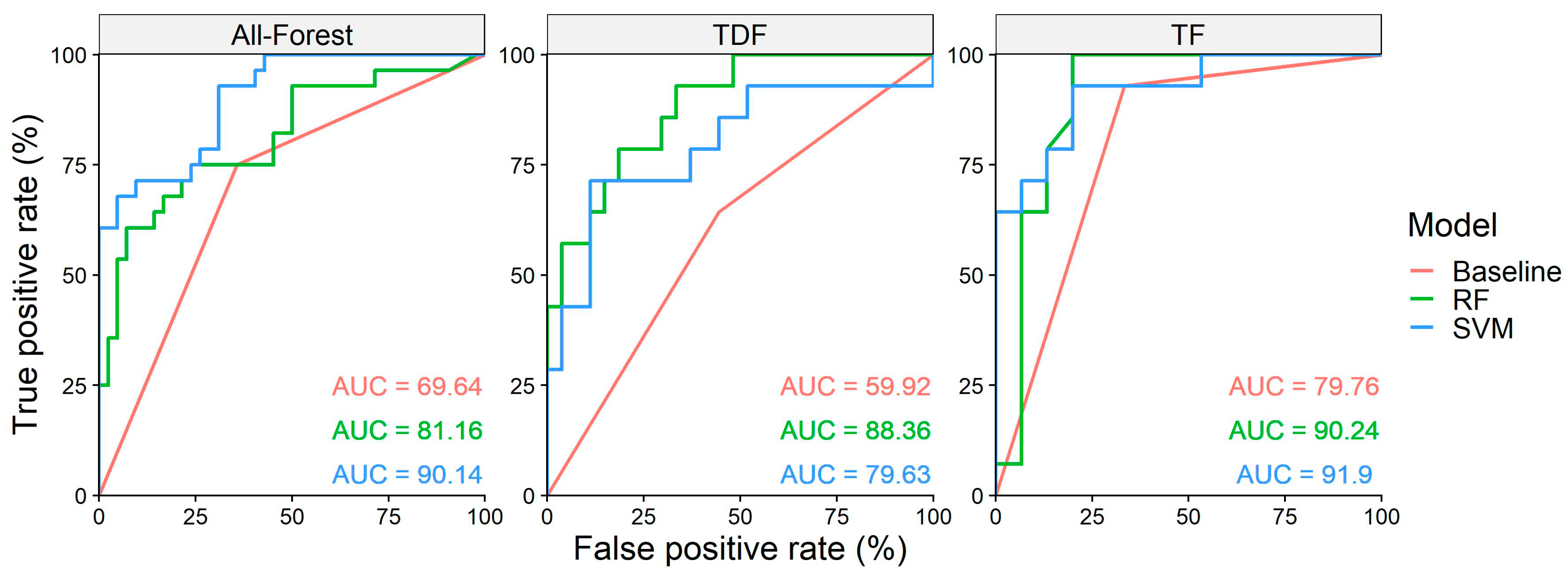
3.4. ROC Curve and AUC

The ROC curves of the models with the highest accuracy indicate that in all cases the models showed a higher AUC than a random guess and less than the perfect model. Additionally, both ML algorithms have a higher AUC than the baseline model. The plot shows the possible combinations of true positive rate and false positive rate given the data. For example, when the true positive rate and the false positive rate are both at one (1, 1), all the validation data are classified as disturbed forest; while the opposite combination of (0, 0) happens when none of the validation data is classified as disturbed forest. All the points between these two extremes show a combination of different true and false positive rates in the detection (Figure 4).

3.5. Forest Disturbance Prediction in the Study Area

The all-forest with the SVM model was used to predict forest disturbance for the complete study area (Figure 5). Evaluated by 624 random points, the prediction obtained an overall accuracy of 94.87%, while the user’s and producer’s accuracy for the disturbance and non-disturbance were between 82.69% and 97.31%. When weighted by the area proportion of each class, the overall accuracy increased to 97.23%, while the producer’s accuracy for forest disturbance was lowered from 86% to 13.77% (

Table 5. Confusion matrix for the accuracy assessment of the classification by the SVM all-forest model for the complete study area; the area-weighted accuracy indices including the producer’s, user’s, and overall accuracy, as well as area estimates for each class are shown. The actual disturbance and non-disturbance are located in the columns, and the predicted disturbance and non-disturbance are located in the rows.

	Non-Disturbance	Disturbance	User’s Accuracy (%)
Non-disturbance	506	14	97.31
Disturbance	18	86	82.69
Producer’s accuracy (%)	96.56	86.00
Overall accuracy (%)	94.87
Area and weighted area estimates
Area proportion (%)	99.48	0.52
Map area (ha)	175,436.37	912.06
Unbiased area estimate (ha)	170,870.94	5477.49
Standard Error (SE)	1246.90	1246.90
Weighted producer’s accuracy (%)	99.91	13.77
Weighted overall accuracy (%)	97.23

). Overall accuracy can be biased by the imbalance in the number of observations between the classes. Therefore, high overall accuracy values can disguise the low classification capabilities for rare classes. Other methods can give further insights into the classification capabilities for both common and rare classes, such as the F1-score. Although the F1-score can give a better idea of the classification capabilities for all the classes, the overall accuracy reports the precision of the entire map. Thus, the two metrics can be used to describe different aspects of the classification performance.

When the accuracy assessment was weighted by area proportion, due to the extremely large area occupied by the non-disturbance class, a small commission error can have a detrimental effect on the area estimation of the disturbance class [48]. In our case, the commission error weighted by the area of the non-disturbance class (99.48%) reduces the producer’s accuracy of the disturbance class from 86% to 13.77%, when weighted by area proportion.

4. Discussion

4.1. Improvement in Disturbance Detection Using Machine Learning Algorithms

This study demonstrates that using ML algorithms and BFAST model components (ML+BFAST) enabled higher accuracy in forest disturbance detection in comparison with the baseline model, which relies only on a magnitude threshold. In all datasets (i.e., all-forest, TDF, TF), the ML algorithms (i.e., SVM or RF) improved the accuracy achieved in the validation dataset, except for SVM with the TF dataset, which obtained the same accuracy as the baseline model (79.31%). Other evaluations reached similar conclusions when using additional BFAST components or ML algorithms to improve the disturbance detection [28,31].

In the all-forest dataset, SVM over-performed RF with a small difference (4.29%). In turn, in both TDF and TF models, RF obtained 4.88–6.90% higher accuracy than SVM. The similar performance of SVM and RF in remote sensing-based classifications has been commonly reported [18,45]. However, it is unclear if there is a particular advantage of one algorithm over the other, as both algorithms can deal with heterogeneous data, data of high dimensionality, and a limited number of observations [18,45].

Compared with the baseline model, ML approaches did not show an advantage when using magnitude as the single predictive variable (Table A2). This suggests that when magnitude is the only variable used, expert knowledge enables a higher accuracy than a ML approach; however, when the number of variables increases, ML algorithms achieved a higher accuracy (Table A2). A prior report on the use of ML and BFAST has shown the advantages of ML over a simple threshold procedure to identify disturbances [28]. In our case, we used a small training sample and therefore, the advantage of expert knowledge vs. ML is still yet to be tested with a larger dataset.

Interestingly, the most accurate model was the one with the all-forest data instead of the forest-type specific models. This seems to contradict the results from previous findings [28,30,31]. However, a smaller sample size in the forest-type specific models may have caused the lower observed accuracies, since the reduction of the size of the training dataset can have repercussions over the accuracy, particularly with an already small dataset [58,59]. Further research is needed to separate the confounding effects of forest type, sample size and data heterogeneity on the accuracy of the tested models. On the other hand, the importance of forest-type as a predictive variable is less than magnitude, trend, and model fitting period; nonetheless, the importance of this variable is relative to the number of predictive variables included in the models. For example, if fewer predictive variables were used, the importance of forest-type would be enhanced. Additionally, because in our study we only included two types of forest over a relatively small area, it is unclear if forest-type might indeed act as an important variable when including a larger variety of forests [31] or with other forest types [60].

In comparison with similar studies, our model had slightly lower accuracy [28,31], which might be related to the data and the data quality. Experiments with better results have used datasets with higher observation density (e.g., MODIS), a harmonized collection from different sensors or data with improved quality through pre-processing with filtering [31,61,62]. Better results have also been reported when using different indices (e.g., NDMI, NDFI, or multiple spectral indices; [7,28,39,42]), or by including SAR together with optical images [60,63].

Reducing the dimensionality of the feature space before training the ML algorithms has been suggested as a necessary preprocess to improve model performance [64]. However, our study used a limited number of predictors, so we used the importance value analysis instead to determine the predictors included in the simplest models, as they offered more critical information for the classification. Additionally, to avoid overfitting, the best model was selected as the one with fewer predictive variables and not significantly different from the model with the highest accuracy.

4.2. Variable Selection

Our results show that magnitude and trend were ranked most important in all the models. Similar results have also been reported [30,31]. Since magnitude represents the difference between the observed and predicted NDVI, disturbances with higher magnitude values represent a larger deviance from a stable trend, and therefore are more likely correspond to a correct disturbance detection [29,39]. On the contrary, lower magnitude values are often related to interannual variations or noise, and they correspond more often to false detection. As for trend, we found that small trend values usually correspond to a long stable period, which facilitates a correct detection; while high trend values (negative or positive) often were fitted either to a short historical data period or very noisy data (Figure 6). Grogan et al. [31] applied a variable of difference in slope (diff.slope) before and after the breakpoint together with amplitude and other variables and found that diff.slope enabled an increase in ROC AUC of 4–0.14% when used with magnitude and depending on forest-type. Thus, trend seems to be the second most important BFAST component to aid in disturbance detection, just after magnitude of change.

Data quality and model fitting period were ranked as either the second or third most important variables. Data quality contributed to accuracy improvement in the RF with TF dataset model in comparison with the baseline model (86.21% vs. 79.31%). The importance of data quality for disturbance detection has also been reported in [7,60]. In turn, the model fitting period is related to the model fitting quality, since models with longer fitting periods are more robust to interannual variation or noise (e.g., in Figure 6A,C). Time series data can have the same percentage of ‘no-data’ values, implying similar data quality, but the ones with a longer model fitting period would normally render better results. We interpret that this is the reason why model fitting period was selected in the SVM all-forest model, instead of data quality.

4.3. Disturbance Area and Rate Estimation

The increase in accuracy of the ML+BFAST compared with the baseline model is small (overall accuracy: 0.14%; area-weighted accuracy: 0.71%). In addition, both the estimated area of forest disturbance and disturbance rate of the ML+BFAST model overlaps with the previous estimate using the baseline model (baseline: 9136.43 ± 5599.49 ha vs. ML+BFAST: 5477.49 ± 1246.90 ha; baseline: 3654.7 ± 2239.8 ha year⁻¹ vs. ML+BFAST: 2191.0 ± 977.6 ha year⁻¹) [30]. However, in both cases, the ML+BFAST model has a smaller standard error, which translates to less uncertainty in the estimated disturbed area and disturbance rate. This is particularly relevant for forest disturbance quantification since it helps reduce uncertainties in estimating carbon and GHG emissions and therefore is significant for REDD+ implementation [1,65].

On the other hand, the results show that regardless of the method (i.e., using magnitude threshold or ML), most of the forest disturbances remain undetected in the final map (see Table 4, mapped disturbance vs. unbiased disturbance area estimate). Therefore, the validation with stratified sampling is essential to estimate the total area of forest disturbance in the study area.

4.4. Study Limitations

Admittedly, the spatial resolution of the Sentinel-2 images might have been too coarse to distinguish fine-scale degradations in the validation process. In these cases, other available imagery such as Google Earth could have been more informative; however, the problem we encountered was that frequently the available images were from very different dates, which introduced uncertainty in distinguishing seasonal changes from actual disturbances. Thus, we prioritized temporal agreement between the comparisons, instead of spatial resolution. A direct consequence of this decision was that fine-scale degradations could remain undetected in the validation process. Therefore, probably most of the detected disturbances correspond to deforestation. Particularly for very seasonal systems, like the one studied here, the availability of freely available images with high spatial and temporal resolution will be critical to help identify and verify fine-scale disturbances.

Another limitation shown by the followed approach is that it lacks a temporal label for each detected disturbance, as the final map only classifies areas into disturbance and non-disturbance in the monitoring period. One way to identify the dates of the disturbances is to consult the breakpoint date of each change detected by BFAST.

5. Conclusions

This study demonstrates that BFAST can benefit from using a machine learning approach to increase its accuracy for disturbance detection, particularly using magnitude of change, trend, and model fitting period. Support vector machines achieved higher accuracy using the all-forest dataset, while random forests over-performed support vector machines in forest-type specific datasets. We found that expert knowledge over-performed machine learning algorithms when using only magnitude as a predictive variable; however, when the number of variables increases, machine learning algorithms performed better than expert knowledge. Since we used a rather small sample size (238 points), the advantage of expert knowledge vs. machine learning algorithm needs to be tested with training data of a larger sample size to be conclusive. Nevertheless, our results suggest that ML algorithms can be used with BFAST to enhance the accuracy achieved to detect disturbances and obtain disturbance area estimates with lower errors. Future studies should address if the advantage of BFAST+ML for disturbance detection is relative to sample size or the scale of disturbances.

References

1. Frolking, S.; Palace, M.W.; Clark, D.B.; Chambers, J.Q.; Shugart, H.H.; Hurtt, G.C. Forest disturbance and recovery: A general review in the context of spaceborne remote sensing of impacts on aboveground biomass and canopy structure. J. Geophys. Res. Biogeosciences 2009, 114, G00E02. [Google Scholar] [CrossRef]
2. van der Werf, G.R.; Morton, D.C.; DeFries, R.S.; Olivier, J.G.J.; Kasibhatla, P.S.; Jackson, R.B.; Collatz, G.J.; Randerson, J.T. CO2 emissions from forest loss. Nat. Geosci. 2009, 2, 737–738. [Google Scholar] [CrossRef]
3. FAO. Assessing Forest Degradation. Towards the Development of Globally Applicable Guidelines; FAO: Roma, Italy, 2011. [Google Scholar]
4. Collins, M.; Knutti, R.; Arblaster, J.; Dufresne, J.-L.; Fichefet, T.; Friedlingstein, P.; Gao, X.; Gutowski, W.J.; Johns, T.; Krinner, G.; et al. Long-term Climate Change: Projections, Commitments and Irreversibility. In Climate Change 2013: The Physical Science Basis. Contribution of Working Group I to the Fifth Assessment Report of the Intergovernmental Panel on Climate Change; Stocker, T.F., Qin, D., Plattner, G.-K., Tignor, M., Allen, S.K., Boschung, J., Nauels, A., Xia, Y., Bex, V., Midgley, P.M., Eds.; Cambridge University Press: Cambridge, UK, 2013. [Google Scholar]
5. Clark, D. The Role of Disturbance in the Regeneration of Neotropical Moist Forests. In Reproductive Ecology of Tropical Forest Plants; Bawa, K.S., Hadley, M., Eds.; UNESCO, Parthenon Publishing Group: Halifax, UK, 1990. [Google Scholar]
6. Chuvieco, E.; Aguado, I.; Salas, J.; García, M.; Yebra, M.; Oliva, P. Satellite Remote Sensing Contributions to Wildland Fire Science and Management. Curr. For. Rep. 2020, 6, 81–96. [Google Scholar] [CrossRef]
7. Dutrieux, L.P.; Jakovac, C.C.; Latifah, S.H.; Kooistra, L. Reconstructing land use history from Landsat time-series: Case study of a swidden agriculture system in Brazil. Int. J. Appl. Earth Obs. Geoinf. 2016, 47, 112–124. [Google Scholar] [CrossRef]
8. FAO. Global Forest Resources Assessment; FAO: Rome, Italy, 2020. [Google Scholar]
9. Vieilledent, G.; Grinand, C.; Rakotomalala, F.A.; Ranaivosoa, R.; Rakotoarijaona, J.R.; Allnutt, T.F.; Achard, F. Combining global tree cover loss data with historical national forest cover maps to look at six decades of deforestation and forest fragmentation in Madagascar. Biol. Conserv. 2018, 222, 189–197. [Google Scholar] [CrossRef]
10. Kennedy, R.E.; Yang, Z.; Cohen, W.B. Detecting trends in forest disturbance and recovery using yearly Landsat time series: 1. LandTrendr—Temporal segmentation algorithms. Remote Sens. Environ. 2010, 114, 2897–2910. [Google Scholar] [CrossRef]
11. Verbesselt, J.; Hyndman, R.; Newnham, G.; Culvenor, D. Detecting trend and seasonal changes in satellite image time series. Remote Sens. Environ. 2010, 114, 106–115. [Google Scholar] [CrossRef]
12. Zhu, Z.; Woodcock, C.E.; Olofsson, P. Continuous monitoring of forest disturbance using all available Landsat imagery. Remote Sens. Environ. 2012, 122, 75–91. [Google Scholar] [CrossRef]
13. Hirschmugl, M.; Gallaun, H.; Dees, M.; Datta, P.; Deutscher, J.; Koutsias, N.; Schardt, M. Methods for Mapping Forest Disturbance and Degradation from Optical Earth Observation Data: A Review. Curr. For. Rep. 2017, 3, 32–45. [Google Scholar] [CrossRef] [Green Version]
14. Schneibel, A.; Stellmes, M.; Röder, A.; Frantz, D.; Kowalski, B.; Haß, E.; Hill, J. Assessment of spatio-temporal changes of smallholder cultivation patterns in the Angolan Miombo belt using segmentation of Landsat time series. Remote Sens. Environ. 2017, 195, 118–129. [Google Scholar] [CrossRef] [Green Version]
15. Chi, M.; Plaza, A.; Benediktsson, J.A.; Sun, Z.; Shen, J.; Zhu, Y. Big Data for Remote Sensing: Challenges and Opportunities. Proc. IEEE 2016, 104, 2207–2219. [Google Scholar] [CrossRef]
16. Xiao, J.; Chevallier, F.; Gomez, C.; Guanter, L.; Hicke, J.A.; Huete, A.R.; Ichii, K.; Ni, W.; Pang, Y.; Rahman, A.F.; et al. Remote sensing of the terrestrial carbon cycle: A review of advances over 50 years. Remote Sens. Environ. 2019, 233, 111383. [Google Scholar] [CrossRef]
17. Mountrakis, G.; Im, J.; Ogole, C. Support vector machines in remote sensing: A review. ISPRS J. Photogramm. Remote Sens. 2011, 66, 247–259. [Google Scholar] [CrossRef]
18. Sheykhmousa, M.; Mahdianpari, M.; Ghanbari, H.; Mohammadimanesh, F.; Ghamisi, P.; Homayouni, S. Support Vector Machine Versus Random Forest for Remote Sensing Image Classification: A Meta-Analysis and Systematic Review. IEEE J. Sel. Top. Appl. Earth Obs. Remote Sens. 2020, 13, 6308–6325. [Google Scholar] [CrossRef]
19. Camargo, F.F.; Sano, E.E.; Almeida, C.M.; Mura, J.C.; Almeida, T. A comparative assessment of machine-learning techniques for land use and land cover classification of the Brazilian tropical savanna using ALOS-2/PALSAR-2 polarimetric images. Remote Sens. 2019, 11, 1600. [Google Scholar] [CrossRef] [Green Version]
20. Grinand, C.; Rakotomalala, F.; Gond, V.; Vaudry, R.; Bernoux, M.; Vieilledent, G. Estimating deforestation in tropical humid and dry forests in Madagascar from 2000 to 2010 using multi-date Landsat satellite images and the random forests classifier. Remote Sens. Environ. 2013, 139, 68–80. [Google Scholar] [CrossRef]
21. Dlamini, W.M. Analysis of deforestation patterns and drivers in Swaziland using efficient Bayesian multivariate classifiers. Modeling Earth Syst. Environ. 2016, 2, 1–14. [Google Scholar] [CrossRef]
22. Ali, I.; Greifeneder, F.; Stamenkovic, J.; Neumann, M.; Notarnicola, C. Review of machine learning approaches for biomass and soil moisture retrievals from remote sensing data. Remote Sens. 2015, 7, 16398–16421. [Google Scholar] [CrossRef] [Green Version]
23. Wu, L.; Li, Z.; Liu, X.; Zhu, L.; Tang, Y.; Zhang, B.; Xu, B.; Liu, M.; Meng, Y.; Liu, B. Multi-type forest change detection using BFAST and monthly landsat time series for monitoring spatiotemporal dynamics of forests in subtropical wetland. Remote Sens. 2020, 12, 341. [Google Scholar] [CrossRef] [Green Version]
24. Xu, Y.; Yu, L.; Peng, D.; Zhao, J.; Cheng, Y.; Liu, X.; Li, W.; Meng, R.; Xu, X.; Gong, P. Annual 30-m land use/land cover maps of China for 1980–2015 from the integration of AVHRR, MODIS and Landsat data using the BFAST algorithm. Sci. China Earth Sci. 2020, 63, 1390–1407. [Google Scholar] [CrossRef]
25. Fang, X.; Zhu, Q.; Ren, L.; Chen, H.; Wang, K.; Peng, C. Large-scale detection of vegetation dynamics and their potential drivers using MODIS images and BFAST: A case study in Quebec, Canada. Remote Sens. Environ. 2018, 206, 391–402. [Google Scholar] [CrossRef]
26. Zhu, Z.; Woodcock, C.E. Continuous change detection and classification of land cover using all available Landsat data. Remote Sens. Environ. 2014, 144, 152–171. [Google Scholar] [CrossRef] [Green Version]
27. Simoes, R.; Camara, G.; Queiroz, G.; Souza, F.; Andrade, P.R.; Santos, L.; Carvalho, A.; Ferreira, K. Satellite Image Time Series Analysis for Big Earth Observation Data. Remote Sens. 2021, 13, 2428. [Google Scholar] [CrossRef]
28. Schultz, M.; Shapiro, A.; Clevers, J.G.P.W.; Beech, C.; Herold, M. Forest cover and vegetation degradation detection in the Kavango Zambezi Transfrontier Conservation area using BFAST monitor. Remote Sens. 2018, 10, 1850. [Google Scholar] [CrossRef] [Green Version]
29. Verbesselt, J.; Zeileis, A.; Herold, M. Near real-time disturbance detection using satellite image time series. Remote Sens. Environ. 2012, 123, 98–108. [Google Scholar] [CrossRef]
30. Gao, Y.; Solórzano, J.V.; Quevedo, A.; Loya-Carrillo, J.O. How BFAST Trend and Seasonal Model Components Affect Disturbance Detection in Tropical Dry Forest and Temperate Forest. Remote Sens. 2021, 2, 2033. [Google Scholar] [CrossRef]
31. Grogan, K.; Pflugmacher, D.; Hostert, P.; Verbesselt, J.; Fensholt, R. Mapping clearances in tropical dry forests using breakpoints, trend, and seasonal components from modis time series: Does forest type matter? Remote Sens. 2016, 8, 657. [Google Scholar] [CrossRef] [Green Version]
32. Watts, L.M.; Laffan, S.W. Effectiveness of the BFAST algorithm for detecting vegetation response patterns in a semi-arid region. Remote Sens. Environ. 2014, 154, 234–245. [Google Scholar] [CrossRef]
33. Trejo, I.; Dirzo, R. Deforestation of seasonally dry tropical forest: A national and local analysis in Mexico. Biol. Conserv. 2000, 94, 133–142. [Google Scholar] [CrossRef]
34. de la Barreda-Bautista, B.; López-Caloca, A.A.; Couturier, S.; Silván-Cárdenas, J.L. Tropical Dry Forests in the Global Picture: The Challenge of Remote Sensing-Based Change Detection in Tropical Dry Environments; Carayannis, E., Ed.; InTech: Rijeka, Croatia, 2011; pp. 231–256. [Google Scholar]
35. GOFC-GOLD. A Sourcebook of Methods and Procedures for Monitoring and Reporting Anthropogenic Greenhouse; GOFC-GOLD Report Version COP21-1; Wageningen University: Wageningen, The Netherlands, 2016; pp. 1–266. [Google Scholar]
36. Jakovac, C.C.; Dutrieux, L.P.; Siti, L.; Peña-Claros, M.; Bongers, F. Spatial and temporal dynamics of shifting cultivation in the middle-Amazonas river: Expansion and intensification. PLoS ONE 2017, 12, e0181092. [Google Scholar] [CrossRef]
37. Cuevas, R.N.N.; Guzmán, H.L. El Bosque Tropical Caducifolio En La Reserva de La Biosfera Sierra Manantlan, Jalisco-Colima, Mexico. Bol. IBUG 1998, 5, 445–491. [Google Scholar]
38. Borrego, A.; Skutsch, M. How Socio-Economic Differences Between Farmers Affect Forest Degradation in Western Mexico. Forests 2019, 10, 893. [Google Scholar] [CrossRef] [Green Version]
39. DeVries, B.; Verbesselt, J.; Kooistra, L.; Herold, M. Robust monitoring of small-scale forest disturbances in a tropical montane forest using Landsat time series. Remote Sens. Environ. 2015, 161, 107–121. [Google Scholar] [CrossRef]
40. Drusch, M.; Del Bello, U.; Carlier, S.; Colin, O.; Fernandez, V.; Gascon, F.; Hoersch, B.; Isola, C.; Laberinti, P.; Martimort, P.; et al. Sentinel-2: ESA’s Optical High-Resolution Mission for GMES Operational Services. Remote Sens. Environ. 2012, 120, 25–36. [Google Scholar] [CrossRef]
41. Hamunyela, E.; Verbesselt, J.; Bruin, S.d.; Herold, M. Monitoring deforestation at sub-annual scales as extreme events in landsat data cubes. Remote Sens. 2016, 8, 651. [Google Scholar] [CrossRef]
42. Schultz, M.; Clevers, J.G.P.W.; Carter, S.; Verbesselt, J.; Avitabile, V.; Quang, H.V.; Herold, M. Performance of vegetation indices from Landsat time series in deforestation monitoring. Int. J. Appl. Earth Obs. Geoinf. 2016, 52, 318–327. [Google Scholar] [CrossRef]
43. Breiman, L. Random Forests. Mach. Learn. 2001, 45, 5–32. [Google Scholar] [CrossRef] [Green Version]
44. Boser, B.; Guyon, I.; Vapnik, V. A Training Algorithm for Optimal Margin Classifiers. In Proceedings of the Fifth Annual Workshop on Computational Learning Theory, Pittsburgh, PA, USA, 27–29 July 1992. [Google Scholar]
45. Dabija, A.; Kluczek, M.; Zagajewski, B.; Raczko, E.; Kycko, M.; Al-Sulttani, A.H.; Tardà, A.; Pineda, L.; Corbera, J. Comparison of support vector machines and random forests for corine land cover mapping. Remote Sens. 2021, 13, 777. [Google Scholar] [CrossRef]
46. Simoes, R.; Picoli, M.C.A.; Camara, G.; Maciel, A.; Santos, L.; Andrade, P.R.; Sánchez, A.; Ferreira, K.; Carvalho, A. Land use and cover maps for Mato Grosso State in Brazil from 2001 to 2017. Sci. Data 2020, 7, 34. [Google Scholar] [CrossRef] [Green Version]
47. Karatzoglou, A.; Smola, A.; Hornik, K.; Zeileis, A. kernlab. An S4 Package for Kernel Methods in R. J. Stat. Softw. 2004, 11, 1–20. [Google Scholar] [CrossRef] [Green Version]
48. Kuhn, M. Caret: Classification and Regression Training. 2021. Available online: https://CRAN.R-project.org/package=caret (accessed on 10 December 2021).
49. Card, D.H. Using Known Map Category Marginal Frequencies To Improve Estimates of Thematic Map Accuracy. Photogramm. Eng. Remote Sens. 1982, 48, 431–439. [Google Scholar]
50. Maxwell, A.E.; Warner, T.A.; Guillén, L.A. Accuracy assessment in convolutional neural network-based deep learning remote sensing studies—Part 2: Recommendations and best practices. Remote Sens. 2021, 13, 2591. [Google Scholar] [CrossRef]
51. Goutte, C.; Gaussier, E. A Probabilistic Interpretation of Precision, Recall and F-Score, with Implication for Evaluation. Lect. Notes Comput. Sci. 2005, 3408, 345–359. [Google Scholar] [CrossRef]
52. Olofsson, P.; Foody, G.M.; Herold, M.; Stehman, S.V.; Woodcock, C.E.; Wulder, M.A. Good practices for estimating area and assessing accuracy of land change. Remote Sens. Environ. 2014, 148, 42–57. [Google Scholar] [CrossRef]
53. Kuhn, M.; Wickham, H. Tidymodels: A Collection of Packages for Modeling and Machine Learning Using Tidyverse Principles. 2020. Available online: https://www.tidymodels.org (accessed on 10 December 2021).
54. Kuhn, M.; Vaughan, D. Yardstick: Tidy Characterizations of Model Performance. 2021. Available online: https://CRAN.R-project.org/package=yardstick (accessed on 10 December 2021).
55. Pebesma, E. Simple Features for R: Standardized Support for Spatial Vector Data. R J. 2018, 10, 439–446. [Google Scholar] [CrossRef] [Green Version]
56. Hijmans, R.J. Raster: Geographic Data Analysis and Modeling. 2021. Available online: https://CRAN.R-project.org/package=raster (accessed on 10 December 2021).
57. Wickham, H.; Averick, M.; Bryan, J.; Chang, W.; D’Agostino McGowan, L.; François, R.; Grolemund, G.; Hayes, A.; Henry, L.; Hester, J.; et al. Tidyverse. J. Open Source Softw. 2019, 4, 1686. [Google Scholar] [CrossRef]
58. Heydari, S.S.; Mountrakis, G. Effect of classifier selection, reference sample size, reference class distribution and scene heterogeneity in per-pixel classification accuracy using 26 Landsat sites. Remote Sens. Environ. 2017, 204, 648–658. [Google Scholar] [CrossRef]
59. Vabalas, A.; Gowen, E.; Poliakoff, E.; Casson, A.J. Machine learning algorithm validation with a limited sample size. PLoS ONE 2019, 14, e0224365. [Google Scholar] [CrossRef]
60. Schultz, M.; Verbesselt, J.; Avitabile, V.; Souza, C.; Herold, M. Error Sources in Deforestation Detection Using BFAST Monitor on Landsat Time Series Across Three Tropical Sites. IEEE J. Sel. Top. Appl. Earth Obs. Remote Sens. 2016, 9, 3667–3679. [Google Scholar] [CrossRef]
61. Geng, L.; Che, T.; Wang, X.; Wang, H. Detecting spatiotemporal changes in vegetation with the BFAST model in the Qilian Mountain region during 2000–2017. Remote Sens. 2019, 11, 103. [Google Scholar] [CrossRef] [Green Version]
62. Roy, D.P.; Kovalskyy, V.; Zhang, H.K.; Vermote, E.F.; Yan, L.; Kumar, S.S.; Egorov, A. Characterization of Landsat-7 to Landsat-8 reflective wavelength and normalized difference vegetation index continuity. Remote Sens. Environ. 2016, 185, 57–70. [Google Scholar] [CrossRef] [PubMed] [Green Version]
63. Hirschmugl, M.; Deutscher, J.; Sobe, C.; Bouvet, A.; Mermoz, S.; Schardt, M. Use of SAR and Optical Time Series for Tropical Forest Disturbance Mapping. Remote Sens. 2020, 12, 727. [Google Scholar] [CrossRef] [Green Version]
64. Ma, W.; Gong, C.; Hu, Y.; Meng, P.; Xu, F. The Hughes Phenomenon in Hyperspectral Classification Based on the Ground Spectrum of Grasslands in the Region around Qinghai Lake. In International Symposium on Photoelectronic Detection and Imaging 2013: Imaging Spectrometer Technologies and Applications; International Society for Optics and Photonics: Bellingham, WA, USA, 2013; Volume 8910, p. 89101G. [Google Scholar] [CrossRef]
65. Herold, M.; Román-Cuesta, R.M.; Mollicone, D.; Hirata, Y.; Van Laake, P.; Asner, G.P.; Souza, C.; Skutsch, M.; Avitabile, V.; MacDicken, K. Options for monitoring and estimating historical carbon emissions from forest degradation in the context of REDD+. Carbon Balance Manag. 2011, 6, 13. [Google Scholar] [CrossRef] [PubMed] [Green Version]
Figure 1. (A) Study area location and spatial distribution of the temperate and tropical dry forest. (B) Illustrations of sample points manually classified as disturbance and non-disturbance in the tropical dry forest (TDF) and temperate forest (TF) using Sentinel-2 natural color composites available in Google Earth Engine. Here the sample points are depicted by circles with yellow outlines.
Remotesensing 14 00803 g001
Figure 2. Flowchart of the method.
Remotesensing 14 00803 g002
Figure 3. Variable importance scaled to a 0–100 range for the random forests (A) and support vector machines (B) models.
Remotesensing 14 00803 g003
Figure 4. ROC curves for the RF and SVM models in the all-forest, TDF, and TF datasets. AUC values are shown in percentages.
Remotesensing 14 00803 g004
Figure 5. Visual comparison of the predicted disturbance by the most accurate models using different datasets. The points indicate the validation data for the disturbance class (orange) and non-disturbance class (blue) (A) Complete study area disturbance prediction using the all-forest baseline model. Examples of the disturbed areas detected using different models and datasets are presented in line; (B) All-forest; (C) Tropical dry forest (TDF); and (D) temperate forest (TF). The three best models are in column 1: Baseline model, 2: random forests (RF), and 3: support vector machines (SVM). The three maps at line B illustrate the disturbance detected by the three models using the all-forest dataset; similarly, the three maps at line C illustrate the disturbance with the TDF dataset and line D with the TF dataset.
Remotesensing 14 00803 g005
Figure 6. Example of areas with correct disturbance detection ((A) TDF and (C) TF) and false detection ((B) TDF and (D) TF) in the baseline model, but correctly classified as non-disturbance in the SVM all-forest model. Each point corresponds to an observed NDVI value in the time series, while its color indicates its correspondence to the historical (green) or monitoring period (red). In turn, the blue solid line shows the model fitted to the data in the historical period and projected to the monitoring window. The dashed lines show the NDVI behavior through time in the historical (green) and monitoring periods (red). Finally, the black dashed line indicates the start of the monitoring period, while the solid yellow line indicates the date of the detected breakpoint.
Remotesensing 14 00803 g006