Spatio-Temporal Quality Indicators for Differential Interferometric Synthetic Aperture Radar Data

Abstract

Satellite-based interferometric synthetic aperture radar (InSAR) is an invaluable technique in the detection and monitoring of changes on the surface of the earth. Its high spatial coverage, weather friendly and remote nature are among the advantages of the tool. The multi-temporal differential InSAR (DInSAR) methods in particular estimate the spatio-temporal evolution of deformation by incorporating information from multiple SAR images. Moreover, opportunities from the DInSAR techniques are accompanied by challenges that affect the final outputs. Resolving the inherent ambiguities of interferometric phases, especially in areas with a high spatio-temporal deformation gradient, represents the main challenge. This brings the necessity of quality indices as important DInSAR data processing tools in achieving ultimate processing outcomes. Often such indices are not provided with the deformation products. In this work, we propose four scores associated with (i) measurement points, (ii) dates of time series, (iii) interferograms and (iv) images involved in the processing. These scores are derived from a redundant set of interferograms and are calculated based on the consistency of the unwrapped interferometric phases in the frame of a least-squares adjustment. The scores reflect the occurrence of phase unwrapping errors and represent valuable input for the analysis and exploitation of the DInSAR results. The proposed tools were tested on 432,311 points, 1795 interferograms and 263 Sentinel-1 single look complex images by employing the small baseline technique in the PSI processing chain, PSIG of the geomatics division of the Centre Tecnològic de Telecomunicacions de Catalunya (CTTC). The results illustrate the importance of the scores—mainly in the interpretation of the DInSAR outputs.

1. Introduction

Advancements in recent synthetic aperture radar (SAR) missions, specifically the introduction of the C-band Sentinel-1 SAR mission with a short revisit time, have boosted the use of differential interferometric SAR (DInSAR) processing and analysis methods to a wide range of remote sensing applications. The DInSAR technique works by exploiting the phase difference between two or more complex-valued SAR images acquired over the same area, taken from slightly different sensor positions [1]. It can detect subtle surface deformations with wide coverage and high spatial resolution [2]. The availability of measurements at all weather conditions and in locations that are inaccessible, remote, or hazardous [3], presents another area of advantage compared to traditional geodetic techniques. Such advantages render the approach applicable for land subsidence [4,5,6] and infrastructure [7] monitoring, and in the analysis of deformations due to mining [8] and volcanic [9] activities, to mention a few. In the past two decades, a broad and significant development has been made. Advances in methods and algorithms for pixel selection, phase unwrapping (PhU), and atmospheric phase component estimation drew greater attention in the scientific community [10]. Development of DInSAR data integration methodologies (with other terrestrial geodetic measurements), use of polarimetric data, the introduction of deep/machine learning techniques are, in addition, receiving more attention very recently. A critical review in the development of DInSAR methodologies including main advantages and limitations are discussed in the research by authors of [1,10,11].

One of the main goals of the advanced DInSAR analysis is obtaining the Time Series (TS) of ground deformations of a target relative to spatial and temporal references. TS analysis methods estimate the temporal evolution of deformation by incorporating information from multiple SAR interferograms [12]. Forming interferogram networks by constraining the spatial and temporal baselines of images presents one method to select pixels coherent in space and time. Generally, for TS analysis, interferograms are generated based on the principle that lies either on a persistent scatterers (PS) [13] approach or on using small baseline interferograms [14], which is intended for incorporating distributed scatterers (DS), or based on a technique combining both PS and DS [15]. Furthermore, following the interferogram selection, points with significant decorrelation effects would be discarded– mostly based on either the criteria of dispersion of amplitude [13] or coherence [16]. The dispersion of amplitude criterion can preserve the full resolution of a SAR image though it results in a low density of PSs, especially in rural areas. On the other hand, the coherence criterion can provide a higher density of PSs in rural areas compared with the former criteria. However, the multi-looking and spatial averaging employed in the coherence calculation affects the resolution of the final outputs, unlike the dispersion of amplitudes criterion. The threshold used in either criterion is a decisive factor and represents a tradeoff between quality and density of points that also highly influences the quality of results. Moreover, target points could be selected based on the temporal coherence criterion [9], the maximum likelihood estimation [17,18], phase stability [19], the polarimetric phase information [20], the coherence matrix derived from the interferograms [21], or based on deep learning networks [22].

Attempts have additionally been made to ensure optimal phase estimation by integer least square (LS) [23], goodness-of-fit [15], adaptive phase optimization [24], and by using corner reflectors to validate phase observations [25,26]. However, the spatio-temporal PhU [27,28] remains yet a challenging and ill-posed problem that possibly leads to the incorrect estimation of deformation TS. Among many others, the phase inversion algorithm based on $L_1$- norm minimization [29] and phase closure technique [30] have been implemented to correct such errors. However, achieving high quality TS is still not straightforward and depends on many factors including the number of available SAR images, density and quality of selected PSs, spatial extent and deformation rates, and the quality and location of the reference point [10]. This highlights the need for DInSAR quality checks as an important part of the processing algorithms. Accordingly, the following section summarizes some of the existing quality indices in TS DInSAR processing.

Quality Indices

The most widely used index is the fit to linear model, also called temporal coherence, which describes how well the interferometric phase observations fit to the linear displacement model. To obtain the index, first the $N$ samples of the TS are transformed from deformations [mm] to phases [rad], obtaining ${\mathsf{\phi }}_{\mathrm{k}}$ for each temporal sample. Then, the corresponding mean velocity is computed from the TS by LS linear fit to get ${\widehat{\mathsf{\phi }}}_{{\mathrm{k}}_{\mathfrak{m}}}$. Finally, the degree-of-fit is calculated based on [13]:

$${\mathsf{\gamma }}_{\tau }=\frac{1}{N}\left|{\displaystyle \sum }_{\mathrm{k}=1}^N{e}^{j\left({\widehat{\mathsf{\phi }}}_{\mathrm{k}}-{\widehat{\mathsf{\phi }}}_{{\mathrm{k}}_{\mathfrak{m}}}\right)}\right|$$

(1)

where ${\widehat{\mathsf{\phi }}}_{\mathrm{k}}$ is the interferometric phase in the $k^{th}$ interferogram after unwrapping and atmospheric-signal mitigation, and ${\widehat{\mathsf{\phi }}}_{{\mathrm{k}}_{\mathfrak{m}}}$ is the estimated phase TS from the model.

The index indicates the quality of the estimated deformation velocities and not the quality of the corresponding deformation TS. It describes measurement noise, model errors and noise due to the scattering property of the PS. However, the dependency of the temporal coherence on a displacement model illustrates a disadvantage and does not allow for distinguishing between measurement noise and deformation model imperfections. Moreover, the dependency of the index on the reference point leads to a decrease in the value of a PS as it gets farther from a reference point, which makes the assessment of the reliability of the delivered results difficult.

Temporal coherence is employed by several research groups and monitoring services. For instance, the European Ground Motion Service [31], the major existing DInSAR-based deformation monitoring service, provides the temporal coherence value of each measurement point along with the estimated standard deviation of the mean velocity computed using variance propagation on the regression model.

Another index is provided by the spatio-temporal consistency (STC) check [32], which is computed for each PS by comparing its behavior in time and space with nearby PSs. It contains a combination of information on the spatial consistency of the TS and the point quality. It is assumed that two close PS points describe the same deformation behavior in time. Therefore, the STC is especially suitable for the analysis of spatially correlated deformation phenomena. The STC at ${\mathfrak{p}}_0$, denoted by ${\rho }_0$, is computed as:

$${\rho }_0=\underset{\forall \mathfrak{p}\in \mathsf{\Omega }}{\min }\frac{\mathsf{\lambda }}{4\mathsf{\pi }}\sqrt{\frac{1}{\mathrm{m}-1}{\displaystyle \sum }_{\mathrm{i}=1}^{\mathrm{m}-1}{\left(\Delta {\mathsf{\phi }}_{\mathfrak{p}}^{\mathrm{i}+1}-\Delta {\mathsf{\phi }}_{{\mathfrak{p}}_0}^{\mathrm{i}+1}\right)}^2} ; \mathrm{where} \Delta {\mathsf{\phi }}_{\mathfrak{p}}^{\mathrm{i}+1}={\mathsf{\phi }}_{\mathfrak{p}}^{\mathrm{i}+1}-{\mathsf{\phi }}_{\mathfrak{p}}^{\mathrm{i}}$$

(2)

$\mathrm{m}$ is the number of SAR image acquisitions, $\lambda$ the radar wavelength and $\mathsf{\phi }$ the unwrapped phase in the TS. $\mathsf{\Omega }$ refers to the neighborhood of ${\mathfrak{p}}_0$ containing all PSs in the annulus satisfying ${\mathrm{r}}_{\min }<\Vert \mathfrak{p}-{\mathfrak{p}}_0\Vert <{\mathrm{r}}_{\max }$.

The minimum radius ${\mathrm{r}}_{\min }$ is set to exclude the inclusion of points that are related to the same physical scatterer, such as, side lobes and the maximum radius ${\mathrm{r}}_{\max }$ is set to prevent the influence of the low-frequency deformation patterns on the quality estimate. This index works well for high point density, but its suitability is in question for sparsely distributed PSs. Therefore, the reliability of the index is spatially variable due to the unequal number of elements of the set $\mathsf{\Omega }$.

The indices described above relate to a single measurement point, and not to the corresponding time stamp of a TS. Obtaining quality indices at the level of TS, i.e., an index for each date of a TS, would be of much importance in the interpretation of TS results. An effort to respond to those limitations was made in [33], though it still lacks breadth. This paper is thus aimed at augmenting and extending previous works by incorporating quality indicators (QIs) not only for the measurement points or TS but also for images and interferograms. These QIs make use of post-PhU estimated residual information and hence are intended to quantify the errors attributed to the PhU. Complementing features such as PSs, interferograms and images with such QIs will help to build trust and confidence in interpretation and decision making based on DInSAR outputs.

The study is limited to internal data QIs for Satellite DInSAR measurements—use of measurement points from other geodetic techniques such as that of GNSS are not the focus of this study. Datasets used in this study are generated by the PSI processing chain, PSIG of the geomatics division of CTTC. The datasets, tools and methods used in the phase estimation and proposed quality indicators are discussed briefly in Section 2 and Section 3. Results and discussions are addressed in Section 4, followed by conclusions and future directions presented in Section 5.

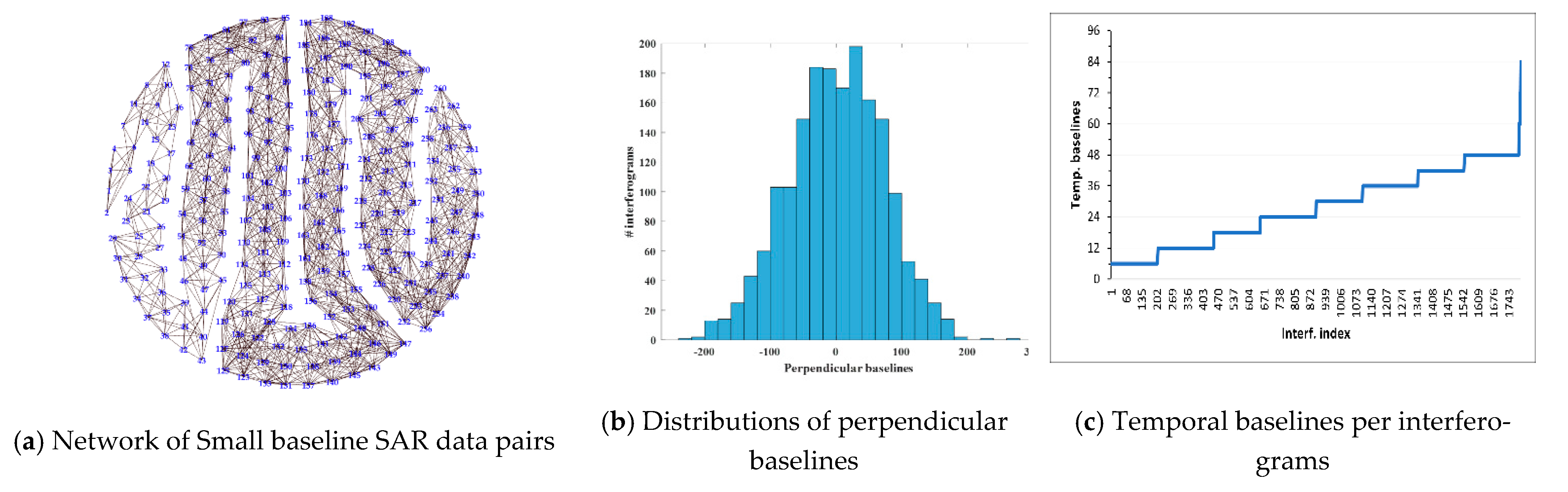
2. Datasets and Tools

The constellation of C-band SAR imaging Sentinel-1 A/B satellites, launched in 2014/16, has brought significant opportunities to the field of interferometric data processing. Operating day and night at all weather conditions along with their free of charge image availability at high temporal acquisition frequency boost their broad remote sensing applications. Unlike many other previous missions, the improvement in the temporal frequency along with recent methodologies [2,14,34] provide relatively dense and coherent signals that could mitigate phase unwrapping errors in the DInSAR TS analysis.

For illustrating the proposed approach, we have used Sentinel-1 SAR datasets—single look complex (SLC) images collected in Interferometric wide swath mode from the Venice lagoon, Italy. The area constitutes a densely urbanized environment, a tourist coastland, and rural areas. The availability of the data sets and richness in land cover types are also among the motivations behind the choice of the case area. For the study, 1795 multi-looked (2 × 10) interferograms were generated by constraining the maximum temporal baseline to 84 days and ±250 m as perpendicular baseline and based on the PSIG processing chain [33] tools from 263 Sentinel-1A/B SLC images (covering the period from October 10, 2014, to May 5, 2020). Sentinel-1A/B SLC images are available at the European Space Agency (ESA) Open Access Data Hub (https://scihub.copernicus.eu) and NASA’s Alaska Satellite Facility platform (https://search.asf.alaska.edu).

Figure 1 below illustrates the temporal and spatial baselines of interferograms used in the small baseline subset (SBAS) processing. From Figure 1a edges correspond to interferograms and nodes to the images. In this network, the redundancy of interferograms ranges from 5 to 16. It gets denser after the launch of Sentinel-1B.

3. Methods

The advanced DInSAR techniques involve simultaneous processing of multiple SAR acquisitions over the same area to reduce errors associated with the deformation estimates. The phase value of a target point in the differential interferograms contains the deformation phase, atmospheric delay phase, DEM error phase, and noise phase. The differential interferometric phase in the direction of a radar line of sight $\Delta {\mathsf{\phi }}_{\mathrm{j}}$ at a point ${\mathfrak{p}}_0$ of the ${\mathrm{j}}^{\mathrm{th}}$ interferogram is thus modelled as:

$$\Delta {\mathsf{\phi }}_{\mathrm{j}}\left({\mathfrak{p}}_0\right)=\Delta {\mathsf{\phi }}_{\mathrm{j}}^{\mathrm{defo}}\left({\mathfrak{p}}_0\right)+\Delta {\mathsf{\phi }}_{\mathrm{j}}^{\mathrm{rte}}\left({\mathfrak{p}}_0\right)+\Delta {\mathsf{\phi }}_{\mathrm{j}}^{\mathrm{atmo}}\left({\mathfrak{p}}_0\right)+\Delta {\mathsf{\phi }}_{\mathrm{j}}^{\mathrm{noise}}\left({\mathfrak{p}}_0\right)+2{\mathrm{k}}_{{\mathfrak{p}}_0}\mathsf{\pi }$$

(3)

where:

• $\Delta {\mathsf{\phi }}^{\mathrm{defo}}=\frac{4\mathsf{\pi }}{\mathsf{\lambda }}{\mathsf{\delta }}_{\mathrm{los}}$ stands for the phase difference resulting from the displacement of the target point that occurred between image acquisitions dates, ${\mathsf{\delta }}_{\mathrm{los}}$ is the component of displacement vector along the line-of-sight direction and λ denotes the radar wavelength.
• $\Delta {\mathsf{\phi }}^{\mathrm{rte}}=-\frac{4\mathsf{\pi }}{\mathsf{\lambda }}\frac{{\mathrm{b}}_{\perp }}{\mathrm{rsin}\vartheta }\Delta \mathrm{h}$ refers the residual topography induced on phase, $\Delta \mathrm{h}$ is the difference in height between the DEM and effective target. ${\mathrm{b}}_{\perp }$ is the interferometric perpendicular baseline, $\vartheta$ is the looking angle and $\mathrm{r}$ the slant-range distance from the sensor to target.
• $\Delta {\mathsf{\phi }}^{\mathrm{atmo}}$ is the phase component due to the variation of a medium of signal propagation between image acquisitions.
• $\Delta {\mathsf{\phi }}^{\mathrm{noise}}$ is for phase noise—due to temporal decorrelation, soil moisture, and thermal noise and in general due to all ambient influence that apport little and uncorrelated variation of phase.
• $\mathrm{k}$ in $2{\mathrm{k}}_{{\mathfrak{p}}_0}\mathsf{\pi }$ is the phase ambiguity due to the wrapped nature of phase measurements.

As the main goal of DInSAR is to reconstruct $\Delta {\mathsf{\phi }}_{\mathrm{j}}^{\mathrm{defo}}$ from $\Delta {\mathsf{\phi }}_{\mathrm{j}}$, various phase components must be separated, which presents a challenging task [35]. To compensate for the residual DEM errors [36] and the atmospheric components from the deformation phases, the method of periodogram followed by a least-squares procedure and spatial low-pass filters along with a temporal high-pass filter are used, respectively. Reconstruction of absolute differential phases from the wrapped phases—called PhU—is another important aspect of the multi-temporal DInSAR. The PhU procedure is formulated to resolve the inherent cycle ambiguities of interferometric phases by adding integer multiples of 2π to the wrapped differential phases [37]. The process represents a crucial and error-prone processing step. The errors could be attributed to high deformation rates, phase noise or isolated pixels. In the PSIG chain, the PhU algorithm involves a spatial 2D PhU using a Minimum Cost Flow method [27] accompanied by a temporal 1D phase estimation procedure. For big datasets, the estimation could be performed in temporal blocks to improve computational time. The estimation is undertaken pointwise in exploiting the temporal evolution of each point to detect and correct errors generated in the 2D PhU [38]. This procedure, which is a type of 2+1D PhU and represents the core of the PSIG chain, is described below.

3.1. Post Unwrapping Phase Estimation

Suppose $\ell$ interferograms are generated from $𝓃$ SAR images acquired in an ordered time sequence ${\left\{t_i\right\}}_{i=0}^{n-1}$ based on the multi-master small baseline principle. Let $\Phi$ be the vector of $\ell$ known unwrapped phases computed from the chronologically ordered master and co-master images. If $\widehat{\phi }$ stands for the vector of $𝓃$ unknown parameters with respect to time $t_0$, its values can be estimated from the system of equations [14]:

$$\mathbf{H}\widehat{\phi }=\Phi$$

(4)

where $H$ stands for the incidence matrix. Assuming $u^T=\left[{\mathrm{u}}_1,{\mathrm{u}}_2,\dots ,{\mathrm{u}}_{\ell }\right]$ and $v^T=\left[{\mathrm{v}}_1,{\mathrm{v}}_2,\dots ,{\mathrm{v}}_{\ell }\right]$ are acquisition time-index vectors, respectively, associated with the master and co-master image pairs used in the interferogram generation, the ${\mathrm{j}}^{\mathrm{th}}$ unwrapped interferogram could be described as:

$${\mathsf{\Phi }}_{\mathrm{j}}=\mathsf{\phi }\left(t_{v_{\mathrm{j}}}\right)-\mathsf{\phi }\left(t_{u_{\mathrm{j}}}\right),\hspace{1em}\forall \mathrm{j}\in [1,\ell ]$$

(5)

For instance, if the first differential interferogram is formed by the first master and the third co-master images, the associated differential interferogram would be ${\mathsf{\Phi }}_1= \mathsf{\phi }\left({\mathrm{t}}_2\right)-\mathsf{\phi }\left({\mathrm{t}}_0\right)$ and similarly if ${\mathsf{\Phi }}_2= \mathsf{\phi }\left({\mathrm{t}}_3\right)-\mathsf{\phi }\left({\mathrm{t}}_1\right)$, the first two rows of the incidence matrix is formulated as in $H$ in the system below:

$$\underset{H}{\underbrace{{\left[\begin{array}{ccccccc}0& 1& 0& 0& \dots & 0& 0\\ -1& 0& 1& 0& \dots & 0& 0\\ ⋮& ⋮& ⋮& ⋮& ⋮& ⋮& ⋮\\ .& .& .& .& .& .& 1\end{array} \right]}_{\ell \times \left(𝓃-1\right)}}}. \underset{\widehat{\mathsf{\phi }}}{\underbrace{{\left[\begin{array}{c}{\widehat{\mathsf{\phi }}}_1\\ {\widehat{\mathsf{\phi }}}_2\\ ⋮\\ {\hat{\mathsf{\phi }}}_{𝓃-1}\end{array} \right]}_{\left(𝓃-1\right)\times 1}}}=\underset{\mathsf{\Phi }}{\underbrace{{\left[\begin{array}{c}{\mathsf{\Phi }}_1\\ {\mathsf{\Phi }}_2\\ ⋮\\ { \mathsf{\Phi }}_{\ell }\end{array} \right]}_{\ell \times 1}}}$$

(6)

${\widehat{\mathsf{\phi }}}_{\mathrm{i}} \mathrm{for} 1\le \mathrm{i}\le 𝓃-1$, denotes the phases at different SAR acquisition dates ${\mathrm{t}}_i$. In the construction of Equation (6) the deformation at the first acquisition date, ${\widehat{\mathsf{\phi }}}_0$ is constrained to be zero to sane the rank of normal matrix (see below). When all the acquisitions belong to a single SBAS block, the incidence matrix $H$ becomes a column rank-full matrix. In which case, the deformation phases are estimated by using the LS approach. If $\mathbf{𝔀}$ is the associated weight matrix, the deformation vector $\widehat{\mathsf{\phi }}$ can be retrieved by solving Equation (7):

$$\widehat{\mathsf{\phi }}\mathbf{=}{\left(H^T\mathbf{𝔀}H\right)}^{-1}{H}^{\mathrm{T}}\mathbf{𝔀}\Phi$$

(7)

If otherwise, differential interferograms belong to different blocks, $H$ becomes rank deficient. This time, the SVD solution derived from the pseudo inverse of matrix $H$ is used to estimate $\widehat{\mathsf{\phi }}$ Equation (8):

$$\widehat{\mathsf{\phi }}\mathbf{=}V{S}^{+}{U}^T\Phi$$

(8)

where $H^{+}=V{S}^{+}{U}^T$ is the pseudo inverse of matrix $H$. U is an orthogonal $\ell \times \ell$ matrix whose first $𝓃$ columns are the eigenvectors of $H{H}^{\mathrm{T}}$; $V$ is an orthogonal $𝓃\times 𝓃$ matrix of columns that are the eigenvectors of $H^{\mathrm{T}}H$, and $S$ is $\ell \times 𝓃$ matrix containing the non-zero singular values of $H$. The solution of the system would be the one that minimizes the $L_2$ norm of both residuals of the system in Equation (4), and that of the estimated phase vector $\widehat{\mathsf{\phi }}$. More information on the SVD is available in [14,39]. In the PSIG approach, a unique block of interferograms is used with redundant observations. The phase estimation algorithm is also accompanied by outlier correction/rejection criterion involving the following steps [33]:

• LS estimation, computing the residuals.
• Temporally removing the highest outlier candidate from the network and performing a new LS estimation. The observation is considered as an outlier candidate when the corresponding residual is greater than the residual threshold.
• Checking the residual of the outlier candidate: if it is a multiple of 2π (within a given tolerance), the observation is corrected and reaccepted. For unwrapping tolerance, ${𝓊}_0$ if an error lies within $2𝓀\pi \pm {𝓊}_0, 𝓀\in \mathbb{Z}$ then it is considered as an unwrapping error and will be corrected. Otherwise, the decision of re-entering or rejecting the outlier candidate is based on the comparison of its old and new residuals.
• The procedure is executed iteratively for each observation until there are no remaining outlier candidates.

Residuals and redundancy of network of interferograms represent the main parameters in the 1D phase estimation step. The redundancy parameter relates the observations vector to the estimated residual vector [33,40] and helps to mitigate the distribution of errors from the LS estimates. The redundancy values are used as indicators of the reliability of observations [27]. Moreover, residuals are useful in the analysis of erroneous interferograms and/or images [33]. The residual of the ${\mathrm{i}}^{th}$ measurement point in the ${\mathrm{j}}^{th}$ interferogram denoted by ${\epsilon }_{ij}$ is computed by taking the difference of the unwrapped interferometric phase ${\mathsf{\Phi }}_{ij}$ and LS estimated phases of the associated master ${\widehat{\mathsf{\phi }}}_{{\mathrm{M}}_{\mathrm{ij}}}$ and co-master ${\widehat{\mathsf{\phi }}}_{{\mathrm{S}}_{\mathrm{ij}}}$ images.

$${\mathsf{\epsilon }}_{\mathrm{ij}}={\mathsf{\Phi }}_{\mathrm{ij}}-\left({\widehat{\mathsf{\phi }}}_{{\mathrm{S}}_{\mathrm{ij}}}-{\widehat{\mathsf{\phi }}}_{{\mathrm{M}}_{\mathrm{ij}}}\right)$$

(9)

In this study, we used the residual information to derive quality indicators for PSs, interferograms, images and for images in a TS based on the following scores.

3.2. Proposed Quality Indicators

QIs would be essential to assess the reliability of DInSAR measurements and to identify and quantify features with uncertainty both spatially and temporally. Accordingly, we have introduced four scores as QIs of measurement points as well as for TS, images and interferograms.

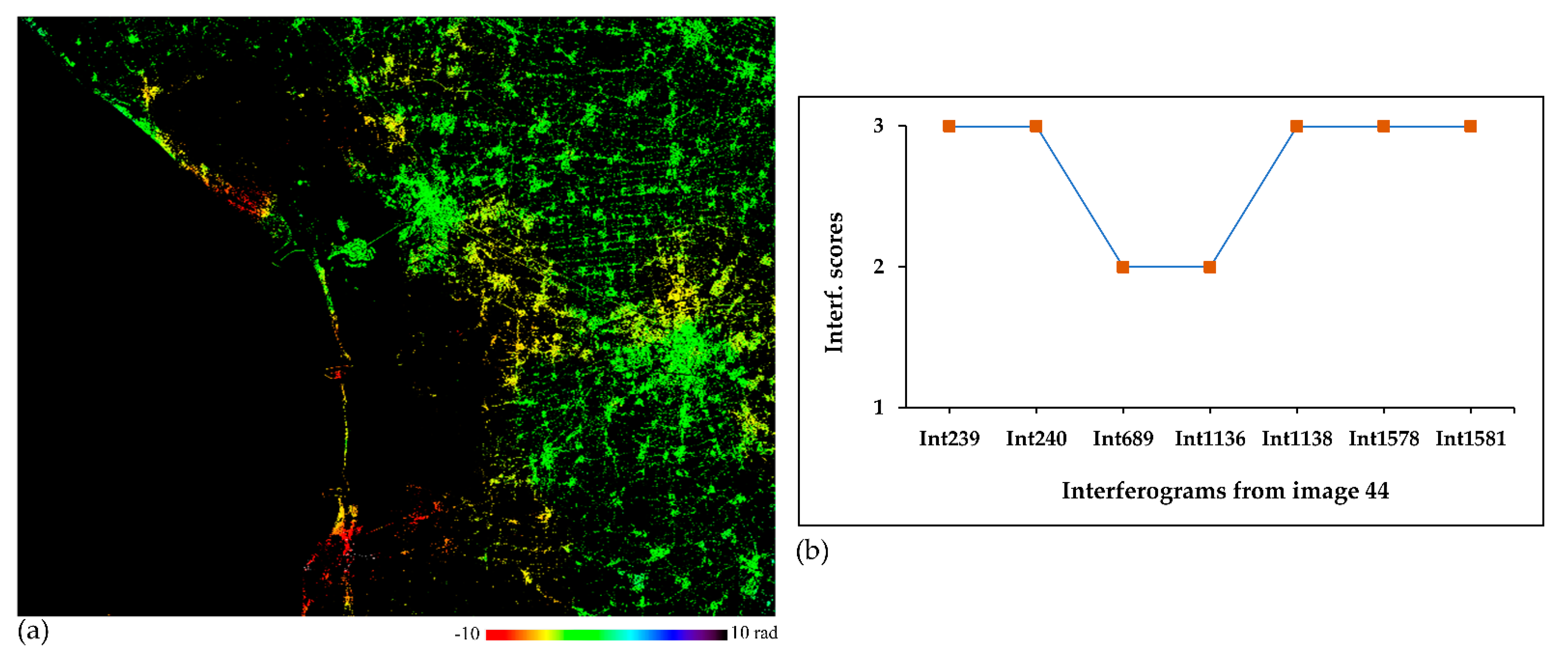
• Interferogram score ($S_{in}$)—a score assigned to interferograms. It indicates the global effect of PhU errors per interferogram. If needed, the interferogram scores would be used to exclude affected interferograms, if any, and hence to update the network and recompute the estimation.
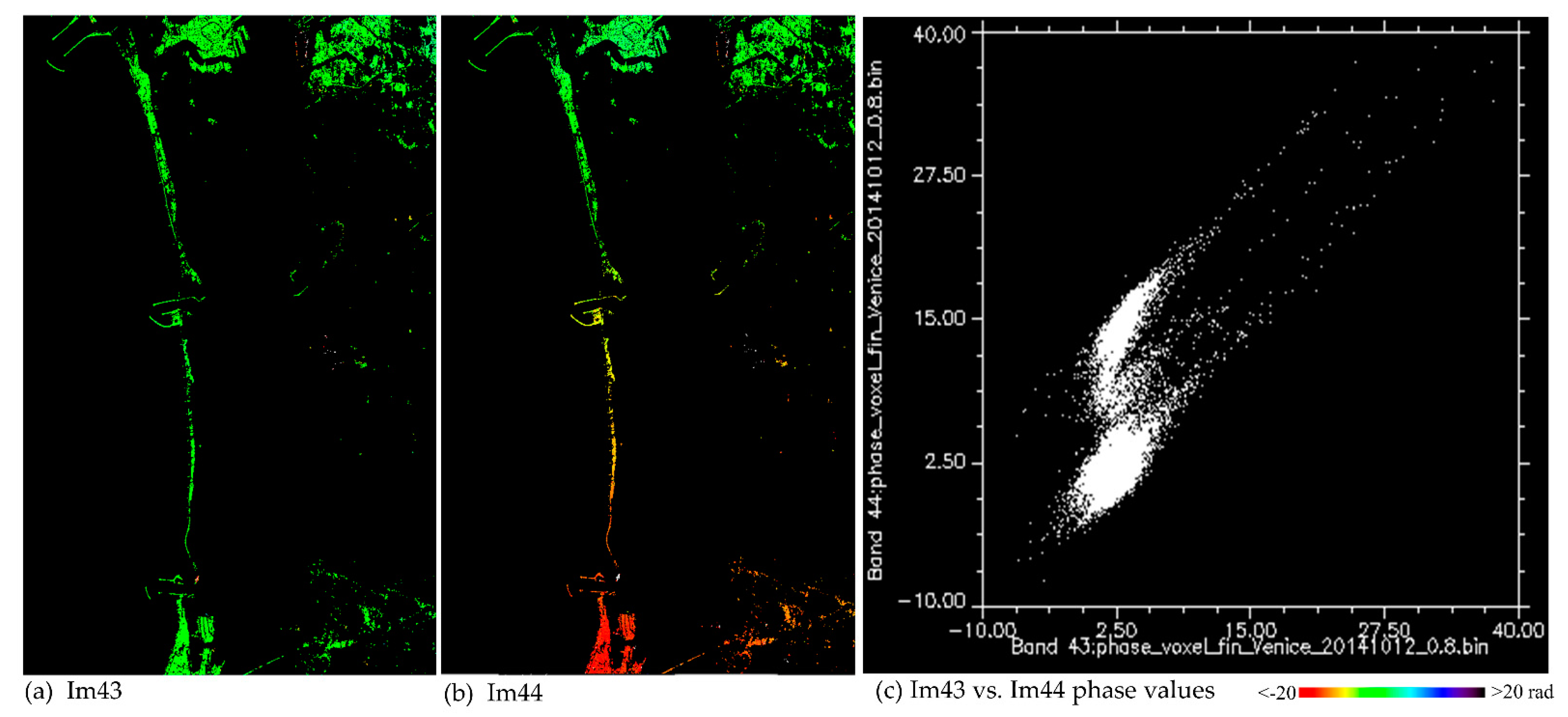
• Image score ($S_{im}$)—a score assigned to images. As with the case of interferograms, ${\mathrm{S}}_{\mathrm{im}}$ shows spatially global effects. This score could also be used to remove one or more images, adjust the network and recompute the estimation.
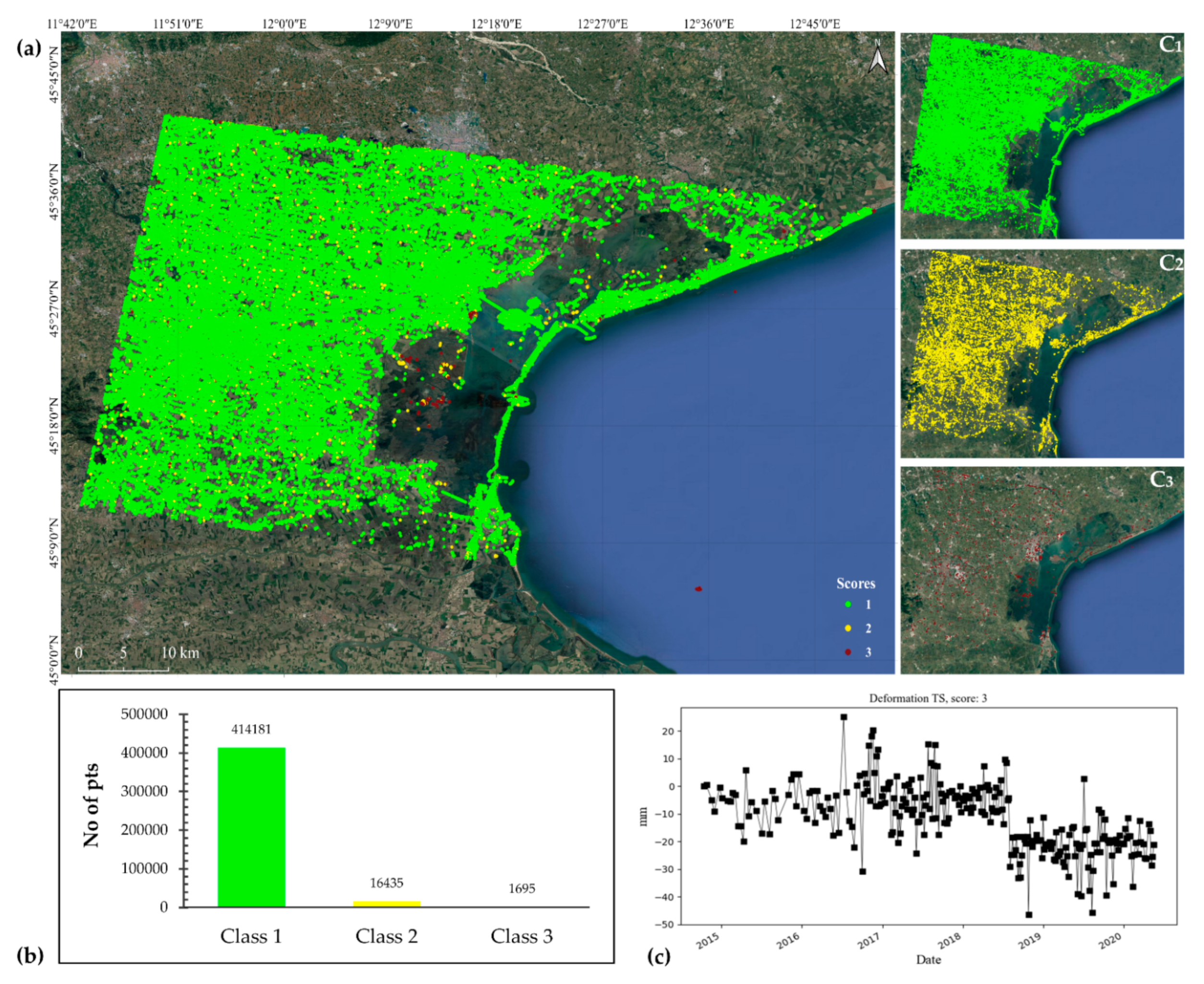
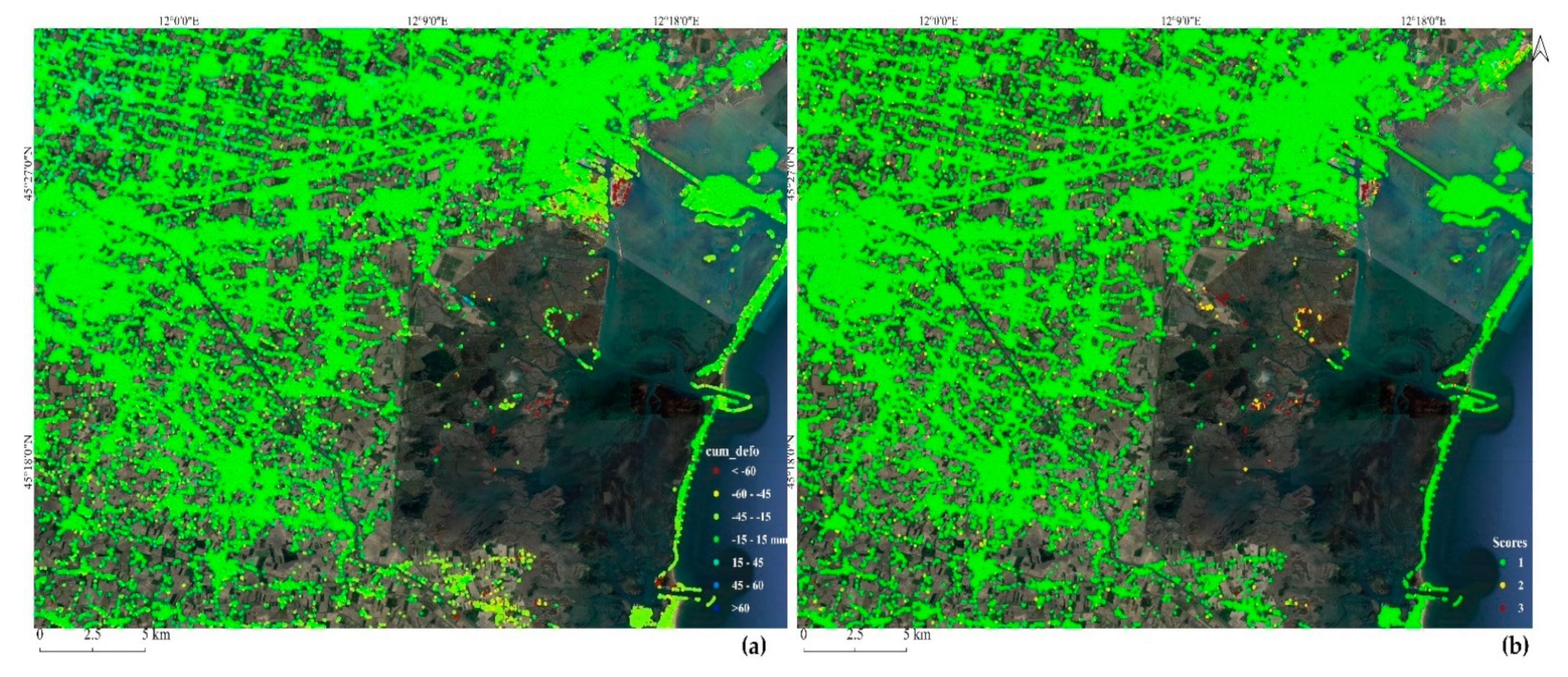
• Point score ($S_{pt}$)—a score assigned to each measurement point. It defines spatially local and temporally global characteristics of a point. The score also provides supplementary information in the interpretation of TS results by separating reliable points from unreliable ones.
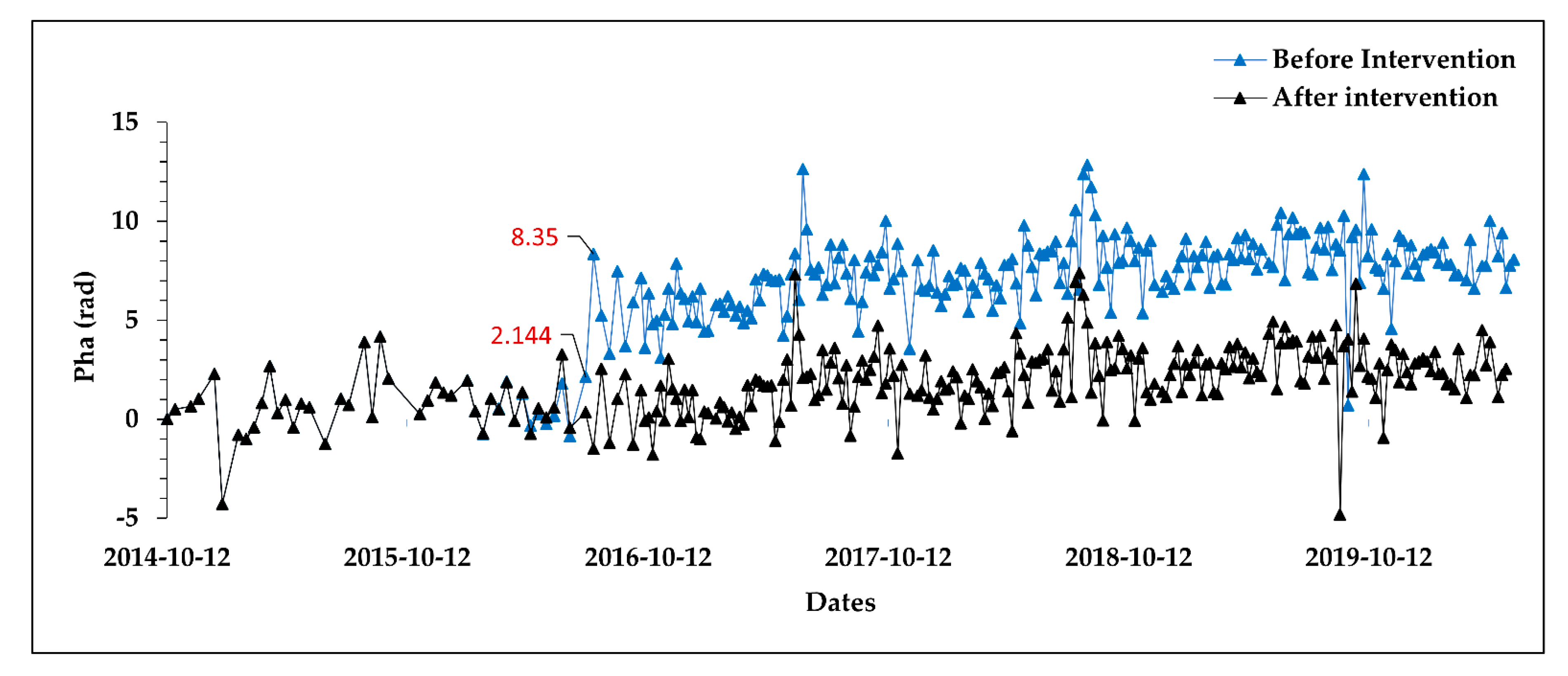
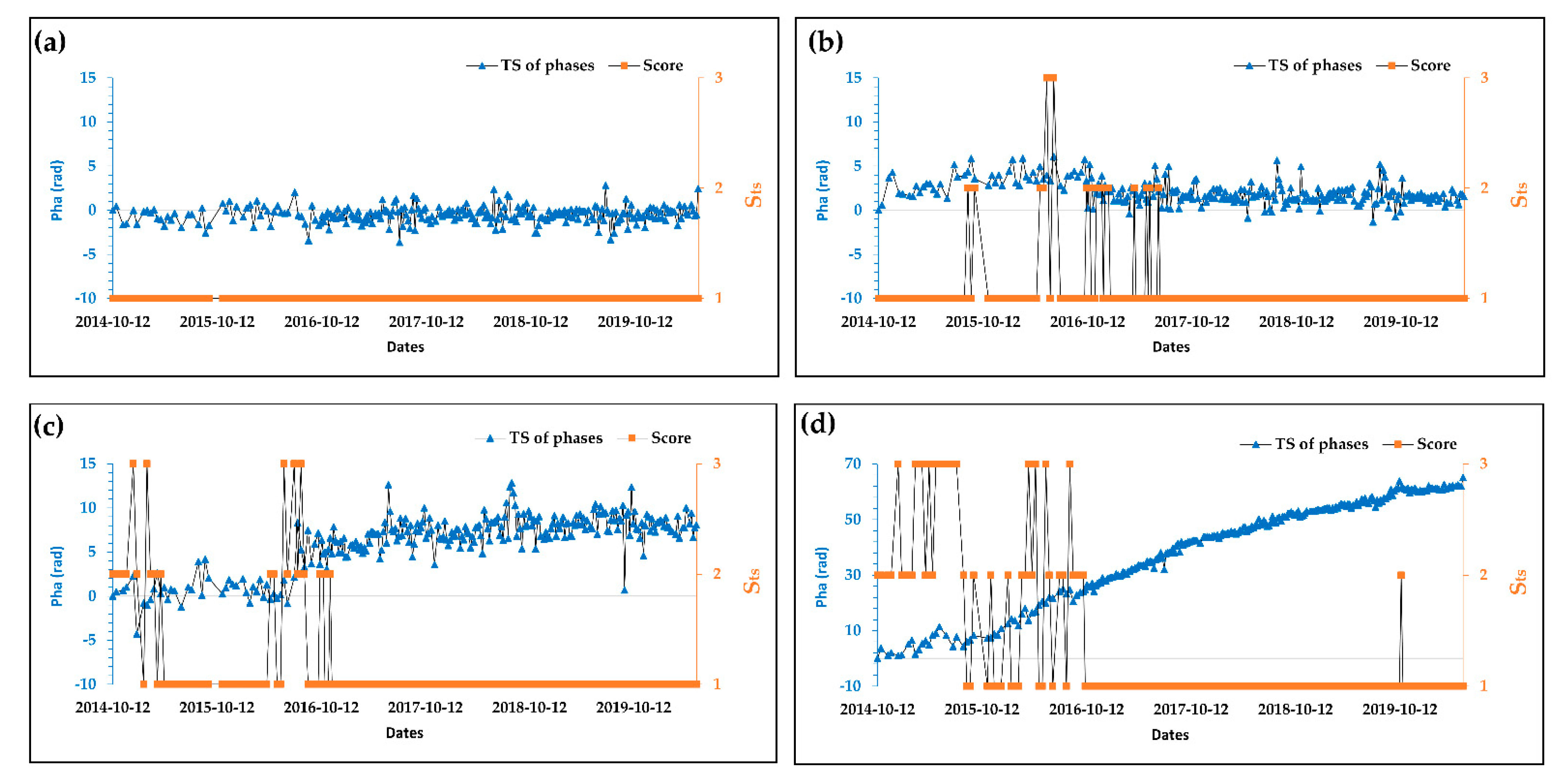
• TS scores ($S_{ts}$)—a detailed score associated with each date of SAR image acquisitions within a given TS of a point. This score indicates temporally local as well as spatially local effects of PhU error influences.

Let $𝓂$, $\ell$ and $𝓃$, respectively, refer to the number of images, the number of interferograms and the number of points processed. Automatic assignment of the above scores for interferograms, images, points and TS thus involves the following steps:

• Computing residuals from the first LS estimation Equation (4).
• Defining a binary matrix of order $n\times \ell$ based on the piecewise function ${\xi }_{ij}$:

  $${\xi }_{ij}=\{\begin{array}{l}1, \mathrm{if} \left|{\epsilon }_{ij}\right|>{\epsilon }_0\\ 0, \mathrm{otherwise} \end{array}$$

  (10)

  for $1\le i\le n$ and $1\le j\le \ell$. While ${\epsilon }_{ij}$ stands for the residual of $i^{th}$ point and ${\mathrm{j}}^{\mathrm{th}}$ interferogram, and ${\epsilon }_0$ denotes the residual threshold.
• Compute a matrix of order $𝓃\times 𝓂$ whose entries are obtained from ${𝓀}_{\mathrm{i}\mathfrak{r}}$ as:

  $${𝓀}_{\mathrm{i}\mathfrak{r}}={\displaystyle \sum }_{\mathrm{j}=1}^{{\mathfrak{q}}_{\mathfrak{r}}}{\xi }_{ij}$$

  (11)

  where ${\mathfrak{q}}_{\mathfrak{r}}$ represents the number of interferograms connected to image $\mathfrak{r}$ in the network.
• Values of the matrix derived in Equation (11) are then multiplied by the corresponding weights assigned per image—multiplicative inverses of the number of interferograms in the network associated with each image.

  $$\mathsf{{\rm B}}={\left[\begin{array}{ccc}{𝓀}_{11}& \cdots & {𝓀}_{1m}\\ ⋮& \ddots & ⋮\\ {𝓀}_{n1}& \cdots & {𝓀}_{nm}\end{array}\right]}_{nxm}\times {\left[\begin{array}{c}{𝓌}_1{}^{-1}\\ ⋮\\ {𝓌}_m{}^{-1}\end{array}\right]}_{mx1}$$

  (12)

  $\underset{\mathrm{j}}{\min }\left\{{𝓌}_{\mathrm{j}}\right\}\ge 4$ for $1\le \mathrm{j}\le \mathrm{m}$ also holds.
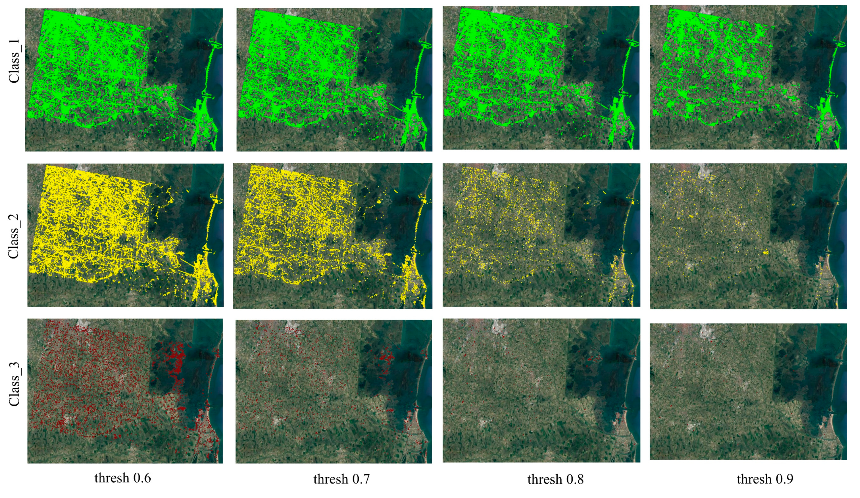
• The resulting weighted matrix $\mathsf{{\rm B}}$, Equation (12), is finally analysed to get scores for PSs and images. These scores correspond to three classes denoted by ${\mathrm{C}}_1$, ${\mathrm{C}}_2$ and ${\mathrm{C}}_3$ that are considered as quality indicators.

By analyzing all points within each of the images, a score providing a global picture on the reliability of the image is assigned. For each $\mathrm{j}$, and $1\le \mathrm{i}\le \mathrm{n}$ the ${\mathrm{j}}^{\mathrm{th}}$ image ${\mathrm{I}}_{\mathrm{j}}$ is assigned to either of the classes—${ \mathrm{C}}_1, { \mathrm{C}}_2$ or ${ \mathrm{C}}_3$ based on Equation (13).

$${ \mathrm{I}}_{\mathrm{j}}\in \{\begin{array}{l}{\mathrm{C}}_3, \mathrm{if} {\displaystyle {\displaystyle \sum }_{\mathrm{i}=1}^{\mathrm{n}}}\left[\frac{{𝓀}_{\mathrm{ij}}}{{𝓌}_{\mathrm{j}}}>{\mathsf{\alpha }}_0\right]>{ \mathsf{\alpha }}_2\\ {\mathrm{C}}_2, \mathrm{if} {\displaystyle {\displaystyle \sum }_{\mathrm{i}=1}^{\mathrm{n}}}\left[\frac{{𝓀}_{\mathrm{ij}}}{{𝓌}_{\mathrm{j}}}>{\mathsf{\alpha }}_1\right]>{ \mathsf{\alpha }}_3\\ { \mathrm{C}}_1, \mathrm{otherwise} \end{array}$$

(13)

The image score is thus the set ${\mathrm{S}}_{\mathrm{im}}=\left\{{\mathrm{I}}_{\mathrm{j}},1\le \mathrm{j}\le \mathrm{m} \right\}$. Similarly, assessing the values of the weighted matrix temporally enables us to judge reliabilities of the score of the ${\mathrm{i}}^{\mathrm{th}}$ point ${\mathfrak{p}}_i$. For instance, for each $\mathrm{i}$, and $1\le \mathrm{j}\le \mathrm{m}$; the ${\mathrm{i}}^{\mathrm{th}}$ point ${\mathfrak{p}}_i$ is assigned to either of the classes based on Equation (14).

$${\mathfrak{p}}_i\in \{\begin{array}{l}{\mathrm{C}}_3, \mathrm{if} {\displaystyle {\displaystyle \sum }_{\mathrm{j}=1}^{\mathrm{m}}}\left[\frac{{𝓀}_{\mathrm{ij}}}{{𝓌}_{\mathrm{j}}}>{\mathsf{\beta }}_0\right]>{ \mathsf{\beta }}_2\\ {\mathrm{C}}_2, \mathrm{if} {\displaystyle {\displaystyle \sum }_{\mathrm{j}=1}^{\mathrm{m}}}\left[\frac{{𝓀}_{\mathrm{ij}}}{{𝓌}_{\mathrm{j}}}>{\mathsf{\beta }}_1\right]>{ \mathsf{\beta }}_3\\ { \mathrm{C}}_1, \mathrm{otherwise} \end{array}$$

(14)

where [.] denotes the Iverson bracket and ${\mathsf{\alpha }}_{𝓈},{\mathsf{\beta }}_{𝓈}, \mathrm{for} 𝓈\in \left\{0,1,2,3\right\}$ are threshold parameters.

The set of all ${\mathfrak{p}}_i$s is the same as the union of the ${\mathrm{C}}_i$s and is given by ${\mathrm{S}}_{\mathrm{pt}}=\left\{{\mathfrak{p}}_{\mathrm{i}},1\le \mathrm{i}\le \mathrm{n} \right\}={{\displaystyle \cup }}_{\mathrm{i}=1}^3{\mathrm{C}}_{\mathrm{i}}$. For the case of interferogram scores, vectors of residuals of measurement points per interferogram at iteration zero would be considered to determine elements of ${\mathrm{S}}_{\mathrm{in}}$. Apart from the difference in the input dataset, the procedures to determine ${\mathrm{S}}_{\mathrm{in}}$ is similar to ${\mathrm{S}}_{\mathrm{im}}$. In the case of ${\mathrm{S}}_{\mathrm{ts}}$ a single measurement point would have as many scores as the length of the TS. At the $i^{th}$ TS a point would be assigned to one of the scores. While ${\mathrm{S}}_{\mathrm{pt}}$ defines whether a point is reliable or not, the ${\mathrm{S}}_{\mathrm{ts}}$ indicates the exact date(s) of concern.

Extensive data analysis and expert judgment have been followed in setting thresholds for assigning the features of interest to different classes automatically. While class ${\mathrm{C}}_1$ is meant to contain the most reliable elements, the elements in ${\mathrm{C}}_3$ are the least reliable. Those elements of ${\mathrm{C}}_3$ could also be excluded from subsequent processing steps if most of the PSs are not in the area of interest. Such action could be considered as part of the PSs selection strategy and would bear an advantage owing to its data reduction effect. On the other hand, detailed investigation—including analysis of possible effects of modifying the network and the resulting temporal baseline on the PhU needs to be made before taking similar measures for an image and interferogram assigned in ${\mathrm{C}}_3$. Scores of PSs can be geocoded and visualized in a GIS environment to ease understanding and interpretation of the spatial distribution of reliable measurement points. Below we discuss results obtained by implementing the tools for the Venice case area, Italy.

4. Results and Discussion

This section illustrates results achieved from the proposed quality scores. The validation of the scores was carried out for 432,311 points, 1795 interferograms and 263 images.

The first quality indicator—the interferograms score,${ \mathrm{S}}_{\mathrm{in}}$ tool was implemented on the residuals of the estimated phases at the first iteration. Generally, the interferograms considered in this study appear acceptable. However, lowering the threshold to 0.4 rad brought in 8% of the total number interferograms into the unreliable class. Figure 2a illustrates one of those interferograms grouped in ${\mathrm{C}}_3$. The second quality indicator—images score, ${\mathrm{S}}_{\mathrm{im}}$ had also justified that unreliable images are those associated with more unreliable interferograms.

Image 44 displays one of the two images classified in the unreliable class from the total of 263 images. Assessing the interferogram scores of this image, we found that five of the seven interferograms associated with image 44 are classified in ${\mathrm{C}}_3$ (Figure 2b). We have also noticed that many of the erroneous measurement points are located in the tourist coastland Sottomarina area—bottom part of the scene in Figure 3b.

Although the temporal gap between images 43 and 44 appear to represent 12 days, phase discontinuities are observed from the 43^rd to the 44^th cumulative phase (Figure 3c). With prior knowledge regarding the nature of the area and based on the phase information, the problem could be attributed to phase unwrapping errors. In line with this, we have explored the phase history of the PSs in the affected area. We discovered that a clear phase unwrapping error occurred in image 44. A phase jump of around 6.21 rad was recorded from 2016-07-09 to 2016-07-21. This particular result has supported the ${\mathrm{S}}_{\mathrm{im}}$ score. We then reprocessed the dataset by excluding those affected images and identified better TS information, as can be seen in Figure 4. The example in the figure justifies the role of the scores in the detection of PhU errors that are not correctly identified by the phase estimation approach.

The third quality indicator is the so-called point score, ${\mathrm{S}}_{\mathrm{pt}}$ tool. In this study, the tool was tested for 432,311 coherent measurement points with a threshold ${\mathsf{\beta }}_0=0.4$. We found that 95.81%, 3.80% and 0.39% of the points were, respectively, classified in ${\mathrm{C}}_1,{ \mathrm{C}}_2$ and ${\mathrm{C}}_3$ classes. This indicates that less than a percent of the processed points is unreliable. The spatial distribution of all scores and those classified in ${\mathrm{C}}_1,{ \mathrm{C}}_2$ and ${\mathrm{C}}_3$ are depicted in Figure 5.

The spatial distribution of the cumulative phase TS was also assessed in addition to the distribution of associated point scores. We have discovered that most of the points classified in ${\mathrm{C}}_3$ are found in and around the Venice lagoon as seen in Figure 6. This is in line with our expectations due to the scattering property of the land cover. Among the elements of ${\mathrm{C}}_3$, the plot in (c) of Figure 5 is a typical example of a TS with PhU error. One of the interesting facts regarding this result is—such TS are classified in the unreliable class by using the residual information at the first iteration of the phase estimation and not by directly using the TS phase information at the final iteration.

For each TS of a PS, we have also generated TS of scores ${\mathrm{S}}_{\mathrm{ts}}$— with each score corresponding to an acquisition date of the SAR image. Below, the TS scores for four of the processed PSs are demonstrated. These scores additionally indicate the reliabilities of a measurement point at a particular date/image. The scores in Figure 7a for instance are all one in the period, justifying the corresponding stable TS. The unwrapping jump in Figure 7c is also captured in the TS score. Moreover, it is worthy of note that score ${\mathrm{C}}_3$ of a TS does not always correspond to unwrapping errors as can be seen on some occasions at plots from (b–d) of Figure 7. The corrections at later iterations of the phase estimation could be a possible cause of such results.

Points Score-$S_{pt}$ for Point Selection

Here we describe how we could utilize the point score, ${\mathrm{S}}_{\mathrm{pt}}$ to set a threshold parameter for measurement point selection in DInSAR processing. For this purpose, the set of coherent measurement points was selected based on the metric shown on Equation (15) [38]. For a point $\mathfrak{p}$ in the azimuth-range plane $A_z\times R_g$, first an estimation of the spatial low-pass interferometric phase $\Delta {\mathsf{\phi }}_{\mathrm{k}}^{\mathrm{LP}}\left(\mathfrak{p}\right)$ is computed using a boxcar averaging window, then the spatial low-pass phase is subtracted modulo-$2\pi$ from the original interferometric phase $\Delta {\mathsf{\phi }}_{\mathrm{k}}\left(\mathfrak{p}\right)$, giving a high-pass estimate of the interferometric phase. For each pixel, the high-pass complex phase vectors are then averaged coherently to mitigate the effect of the phase noise—and the resulting metric is computed by taking the modulus of the resultant vector as:

$$\mathsf{\Omega }\left(\mathfrak{p}\right)=\frac{1}{\ell }\left|{\displaystyle \sum }_{\mathrm{k}=1}^{\ell }\exp [\mathrm{j}\left(\Delta {\mathsf{\phi }}_{\mathrm{k}}\left(\mathfrak{p}\right)-\Delta {\mathsf{\phi }}_{\mathrm{k}}^{\mathrm{LP}}\left(\mathfrak{p}\right)\right]\right|$$

(15)

where $\ell$ is the number of interferograms, and k is the interferogram index. The values of $\mathsf{\Omega }$ range between 0 and 1 inclusive. The higher the value of $\mathsf{\Omega }$ the more coherent the measurement point would be.

First, we tested the point selection on a representative subset of the case area by setting $\mathsf{\Omega }$ thresholds to 0.6, 0.7, 0.8 and 0.9 and we got the results in Figure 8.

To select the appropriate threshold, we used the labelling performance criteria Equation (16) derived based on the ${\mathrm{S}}_{\mathrm{pt}}$ information. The labelling performance indicates the percentage of points labelled in the more reliable group. The higher the value of $\mathfrak{q}$ the better the set of points involved in the processing would be.

$$\mathfrak{q}=\left(1-\frac{{\mathsf{\alpha }}_2{\mathrm{c}}_2+{\mathsf{\alpha }}_3{\mathrm{c}}_3}{{\mathsf{\alpha }}_1{\mathrm{c}}_1}\right)*100\%$$

(16)

where ${\mathrm{c}}_{\mathrm{i}}$ and ${\alpha }_i, 1\le i\le 3$ denotes the number of points in each class and associated weights, respectively. For this experiment, we obtained $\mathfrak{q}\ge 95\%$ as an acceptable range. Accordingly, we found the results by 0.8 and 0.9 thresholds in the range, and selected the former as a convenient choice due to the density of PSs (Figure 9). The decision to pick the right threshold parameter should also depend on the effect of the parameter on the PhU steps. The approach could be taken as an extended points selection technique. It can additionally be used along with other pixel selection criteria.

5. Conclusions

In this paper, we introduced quality indicator tools to multi-temporal DInSAR outputs based on post-PhU phase estimation residual information. Key features of the proposed technique include four scores used to quantify the reliabilities of measurement points, images in a TS, images and interferograms. The techniques proposed are applied pixel by pixel in space and time to associate reliability scores highlighting the influence of PhU errors. Moreover, the tools are valuable in quantifying spatially and temporally global and local effects of phase estimation errors. The results highlight the importance of the proposed quality indicators mainly for data reduction and in assisting the interpretation of TS outputs. We believe the tool will contribute its part at such a high time to integrate quality checks with DInSAR processing chains. Additionally, it is worth noting that the proposed tools are only applicable for multi-master redundant networks. Besides, more work is required in identifying errors due to phase unwrapping from errors attributed to other sources—including those from atmospheric artefacts. Thus, we have envisioned an upgrading of the depth and breadth of the tools mainly in improving the accuracy and compatibility for more processing chains.

References

- Pepe, A.; Calò, F. A Review of Interferometric Synthetic Aperture RADAR (InSAR) Multi-Track Approaches for the Retrieval of Earth’s Surface Displacements. Appl. Sci. 2017, 7, 1264. [Google Scholar] [CrossRef] [Green Version]
- Duan, W.; Zhang, H.; Wang, C.; Tang, Y. Multi-Temporal InSAR Parallel Processing for Sentinel-1 Large-Scale Surface Deformation Mapping. Remote Sens. 2020, 12, 3749. [Google Scholar] [CrossRef]
- Parker, A.L. InSAR Observations of Ground Deformation; Springer Theses; Springer International Publishing: Cham, Germany, 2017; ISBN 978-3-319-39033-8. [Google Scholar]
- Zhang, B.; Wang, R.; Deng, Y.; Ma, P.; Lin, H.; Wang, J. Mapping the Yellow River Delta land subsidence with multitemporal SAR interferometry by exploiting both persistent and distributed scatterers. ISPRS J. Photogramm. Remote Sens. 2019, 148, 157–173. [Google Scholar] [CrossRef]
- Wang, B.; Zhao, C.; Zhang, Q.; Peng, M. Sequential InSAR Time Series Deformation Monitoring of Land Subsidence and Rebound in Xi’an, China. Remote Sens. 2019, 11, 2854. [Google Scholar] [CrossRef] [Green Version]
- Ranjgar, B.; Razavi-Termeh, S.V.; Foroughnia, F.; Sadeghi-Niaraki, A.; Perissin, D. Land Subsidence Susceptibility Mapping Using Persistent Scatterer SAR Interferometry Technique and Optimized Hybrid Machine Learning Algorithms. Remote Sens. 2021, 13, 1326. [Google Scholar] [CrossRef]
- Di Martire, D.; Iglesias, R.; Monells, D.; Centolanza, G.; Sica, S.; Ramondini, M.; Pagano, L.; Mallorquí, J.J.; Calcaterra, D. Comparison between Differential SAR interferometry and ground measurements data in the displacement monitoring of the earth-dam of Conza della Campania (Italy). Remote Sens. Environ. 2014, 148, 58–69. [Google Scholar] [CrossRef]
- Yang, Z.; Li, Z.; Zhu, J.; Wang, Y.; Wu, L. Use of SAR/InSAR in Mining Deformation Monitoring, Parameter Inversion, and Forward Predictions: A Review. IEEE Geosci. Remote Sens. Mag. 2020, 8, 71–90. [Google Scholar] [CrossRef]
- Hooper, A.; Zebker, H.; Segall, P.; Kampes, B. A new method for measuring deformation on volcanoes and other natural terrains using InSAR persistent scatterers. Geophys. Res. Lett. 2004, 31, 1–5. [Google Scholar] [CrossRef]
- Crosetto, M.; Monserrat, O.; Cuevas-González, M.; Devanthéry, N.; Crippa, B. Persistent Scatterer Interferometry: A review. ISPRS J. Photogramm. Remote Sens. 2016, 115, 78–89. [Google Scholar] [CrossRef] [Green Version]
- Gens, R.; Van Genderen, J.L. Review Article SAR interferometry—issues, techniques, applications. Int. J. Remote Sens. 1996, 17, 1803–1835. [Google Scholar] [CrossRef]
- Shanker, P.; Casu, F.; Zebker, H.A.; Lanari, R. Comparison of Persistent Scatterers and Small Baseline Time-Series InSAR Results: A Case Study of the San Francisco Bay Area. IEEE Geosci. Remote Sens. Lett. 2011, 8, 592–596. [Google Scholar] [CrossRef]
- Ferretti, A.; Prati, C.; Rocca, F. Permanent scatterers in SAR interferometry. IEEE Trans. Geosci. Remote Sens. 2001, 39, 8–20. [Google Scholar] [CrossRef]
- Berardino, P.; Fornaro, G.; Lanari, R.; Sansosti, E. A new algorithm for surface deformation monitoring based on small baseline differential SAR interferograms. IEEE Trans. Geosci. Remote Sens. 2002, 40, 2375–2383. [Google Scholar] [CrossRef] [Green Version]
- Ferretti, A.; Fumagalli, A.; Novali, F.; Prati, C.; Rocca, F.; Rucci, A. A New Algorithm for Processing Interferometric Data-Stacks: SqueeSAR. IEEE Trans. Geosci. Remote Sens. 2011, 49, 3460–3470. [Google Scholar] [CrossRef]
- Touzi, R.; Lopes, A.; Bruniquel, J.; Vachon, P.W. Coherence estimation for SAR imagery. IEEE Trans. Geosci. Remote Sens. 1999, 37, 135–149. [Google Scholar] [CrossRef] [Green Version]
- Shanker, P.; Zebker, H. Persistent scatterer selection using maximum likelihood estimation. Geophys. Res. Lett. 2007, 34. [Google Scholar] [CrossRef]
- Zhao, C.; Li, Z.; Zhang, P.; Tian, B.; Gao, S. Improved maximum likelihood estimation for optimal phase history retrieval of distributed scatterers in InSAR stacks. IEEE Access 2019, 7, 186319–186327. [Google Scholar] [CrossRef]
- Hooper, A.; Segall, P.; Zebker, H. Persistent scatterer interferometric synthetic aperture radar for crustal deformation analysis, with application to Volcán Alcedo, Galápagos. J. Geophys. Res. Solid Earth 2007, 112. [Google Scholar] [CrossRef] [Green Version]
- Samsonov, S.; Tiampo, K. Polarization phase difference analysis for selection of persistent scatterers in SAR interferometry. IEEE Geosci. Remote Sens. Lett. 2011, 8, 331–335. [Google Scholar] [CrossRef]
- Navneet, S.; Kim, J.W. A new InSAR persistent scatterer selection technique using top eigenvalue of coherence matrix. IEEE Trans. Geosci. Remote Sens. 2018, 56, 1969–1978. [Google Scholar] [CrossRef]
- Tiwari, A.; Narayan, A.B.; Dikshit, O. Deep learning networks for selection of measurement pixels in multi-temporal SAR interferometric processing. ISPRS J. Photogramm. Remote Sens. 2020, 166, 169–182. [Google Scholar] [CrossRef]
- Samiei-Esfahany, S.; Martins, J.E.; van Leijen, F.; Hanssen, R.F. Phase Estimation for Distributed Scatterers in InSAR Stacks Using Integer Least Squares Estimation. IEEE Trans. Geosci. Remote Sens. 2016, 54, 5671–5687. [Google Scholar] [CrossRef] [Green Version]
- Li, S.; Zhang, S.; Li, T.; Gao, Y.; Chen, Q.; Zhang, X. An Adaptive Phase Optimization Algorithm for Distributed Scatterer Phase History Retrieval. IEEE J. Sel. Top. Appl. Earth Obs. Remote Sens. 2021, 14, 3914–3926. [Google Scholar] [CrossRef]
- Luzi, G.; Espín-López, P.F.; Pérez, F.M.; Monserrat, O.; Crosetto, M. A low-cost active reflector for interferometric monitoring based on sentinel-1 sar images. Sensors 2021, 21, 2008. [Google Scholar] [CrossRef]
- Marinkovic, P.; Ketelaar, G.; Van Leijen, F.; Hanssen, R. InSAR quality control: Analysis of five years of corner reflector time series. In Proceedings of the Fringe 2007 Workshop (ESA SP-649), Frascati, Italy, 26–30 November 2007. [Google Scholar]
- Costantini, M.; Farina, A.; Zirilli, F. A fast phase unwrapping algorithm for SAR interferometry. IEEE Trans. Geosci. Remote Sens. 1999, 37, 452–460. [Google Scholar] [CrossRef]
- Marano, S.; Palmieri, F.; Franceschetti, G. Discrete Green’s methods and their application to two-dimensional phase unwrapping. J. Opt. Soc. Am. A 2002, 19, 1319–1333. [Google Scholar] [CrossRef]
- Lauknes, T.R.; Zebker, H.A.; Larsen, Y. InSAR deformation time series using an L1-norm small-baseline approach. IEEE Trans. Geosci. Remote Sens. 2011, 49, 536–546. [Google Scholar] [CrossRef] [Green Version]
- Benoit, A.; Pinel-Puysségur, B.; Jolivet, R.; Lasserre, C. CorPhU: An algorithm based on phase closure for the correction of unwrapping errors in SAR interferometry. Geophys. J. Int. 2020, 221, 1959–1970. [Google Scholar] [CrossRef] [Green Version]
- Crosetto, M.; Solari, L.; Balasis-Levinsen, J.; Bateson, L.; Casagli, N.; Frei, M.; Oyen, A.; Moldestad, D.A.; Mróz, M. Deformation monitoring at European scale: The copernicus ground motion service. Int. Arch. Photogramm. Remote Sens. Spat. Inf. Sci. 2021, 43, 141–146. [Google Scholar] [CrossRef]
- Hanssen, R.F.; Van Leijen, F.J.; Van Zwieten, G.J.; Bremmer, C.; Dortland, S.; Kleuskens, M. Validation of Existing Processing Chains in TerraFirma Stage 2; Product Validation: Validation in the Amsterdam and Alkmaar Area; ESA TerraFirma Report ESRIN Contract No. 19366//05/I-E; Delft University of Technology: Delft, The Netherlands, 2008. [Google Scholar]
- Devanthéry, N.; Crosetto, M.; Monserrat, O.; Cuevas-González, M.; Crippa, B. An Approach to Persistent Scatterer Interferometry. Remote Sens. 2014, 6, 6662–6679. [Google Scholar] [CrossRef] [Green Version]
- Liu, F.; Pan, B. A New 3-D Minimum Cost Flow Phase Unwrapping Algorithm Based on Closure Phase. IEEE Trans. Geosci. Remote Sens. 2020, 58, 1857–1867. [Google Scholar] [CrossRef]
- Maubant, L.; Pathier, E.; Daout, S.; Radiguet, M.; Doin, M.-P.; Kazachkina, E.; Kostoglodov, V.; Cotte, N.; Walpersdorf, A. Independent Component Analysis and Parametric Approach for Source Separation in InSAR Time Series at Regional Scale: Application to the 2017–2018 Slow Slip Event in Guerrero (Mexico). J. Geophys. Res. Solid Earth 2020, 125. [Google Scholar] [CrossRef]
- Biescas, E.; Crosetto, M.; Agudo, M.; Monserrat, O.; Crippa, B. Two Radar Interferometric Approaches to Monitor Slow and Fast Land Deformation. J. Surv. Eng. 2007, 133, 66–71. [Google Scholar] [CrossRef]
- Ajourlou, P.; Samiei Esfahany, S.; Safari, A. A new strategy for phase unwrapping in InSAR time series over areas with high deformation rate: Case study on the southern Tehran subsidence. Int. Arch. Photogramm. Remote Sens. Spat. Inf. Sci. 2019, 42, 35–40. [Google Scholar] [CrossRef] [Green Version]
- Pepe, A.; Lanari, R. On the Extension of the Minimum Cost Flow Algorithm for Phase Unwrapping of Multitemporal Differential SAR Interferograms. IEEE Trans. Geosci. Remote Sens. 2006, 44, 2374–2383. [Google Scholar] [CrossRef]
- Golub, G.H.; Van Loan, C.F. Matrix Computations, 4th ed.; JHU Press: Baltimore, ML, USA, 2013; ISBN 978-1-4214-0794-4. [Google Scholar]
- Afsharnia, H.; Arefi, H.; Sharifi, M.A. Optimal weight design approach for the geometrically-constrained matching of satellite stereo images. Remote Sens. 2017, 9, 965. [Google Scholar] [CrossRef] [Green Version]
Publisher’s Note: MDPI stays neutral with regard to jurisdictional claims in published maps and institutional affiliations. |
© 2022 by the authors. Licensee MDPI, Basel, Switzerland. This article is an open access article distributed under the terms and conditions of the Creative Commons Attribution (CC BY) license (https://creativecommons.org/licenses/by/4.0/).
Share and Cite
Wassie, Y.; Mirmazloumi, S.M.; Crosetto, M.; Palamà, R.; Monserrat, O.; Crippa, B. Spatio-Temporal Quality Indicators for Differential Interferometric Synthetic Aperture Radar Data. Remote Sens. 2022, 14, 798. https://doi.org/10.3390/rs14030798
Wassie Y, Mirmazloumi SM, Crosetto M, Palamà R, Monserrat O, Crippa B. Spatio-Temporal Quality Indicators for Differential Interferometric Synthetic Aperture Radar Data. Remote Sensing. 2022; 14(3):798. https://doi.org/10.3390/rs14030798
Chicago/Turabian StyleWassie, Yismaw, S. Mohammad Mirmazloumi, Michele Crosetto, Riccardo Palamà, Oriol Monserrat, and Bruno Crippa. 2022. "Spatio-Temporal Quality Indicators for Differential Interferometric Synthetic Aperture Radar Data" Remote Sensing 14, no. 3: 798. https://doi.org/10.3390/rs14030798
APA StyleWassie, Y., Mirmazloumi, S. M., Crosetto, M., Palamà, R., Monserrat, O., & Crippa, B. (2022). Spatio-Temporal Quality Indicators for Differential Interferometric Synthetic Aperture Radar Data. Remote Sensing, 14(3), 798. https://doi.org/10.3390/rs14030798