Spatiotemporal Hybrid Random Forest Model for Tea Yield Prediction Using Satellite-Derived Variables

Abstract

Crop yield forecasting is critical for enhancing food security and ensuring an appropriate food supply. It is critical to complete this activity with high precision at the regional and national levels to facilitate speedy decision-making. Tea is a big cash crop that contributes significantly to economic development, with a market of USD 200 billion in 2020 that is expected to reach over USD 318 billion by 2025. As a developing country, Bangladesh can be a greater part of this industry and increase its exports through its tea yield and production with favorable climatic features and land quality. Regrettably, the tea yield in Bangladesh has not increased significantly since 2008 like many other countries, despite having suitable climatic and land conditions, which is why quantifying the yield is imperative. This study developed a novel spatiotemporal hybrid DRS–RF model with a dragonfly optimization (DR) algorithm and support vector regression (S) as a feature selection approach. This study used satellite-derived hydro-meteorological variables between 1981 and 2020 from twenty stations across Bangladesh to address the spatiotemporal dependency of the predictor variables for the tea yield (Y). The results illustrated that the proposed DRS–RF hybrid model improved tea yield forecasting over other standalone machine learning approaches, with the least relative error value (11%). This study indicates that integrating the random forest model with the dragonfly algorithm and SVR-based feature selection improves prediction performance. This hybrid approach can help combat food risk and management for other countries.

1. Introduction

Tea is the most popular beverage globally after water and has had a price increase of USD 0.05 per kg since the beginning of 2021. China is the leading producer of tea, producing approximately 2.79 million metric tonnes in 2019, followed by India (1.39 M metric tonnes), Kenya (0.45 M metric tonnes), Sri Lanka (0.30 M metric tonnes), and Indonesia (0.13 M metric tonnes) [1,2]. As tea consumption increases every year due to the increase in population in Bangladesh, most of the tea produced meets the national demand [3]. Bangladesh annually earns around BDT 1.775 billion, which is 0.81% of the GDP (Gross Domestic Product) in foreign currency in the export of tea [4]. Despite the involvement of about 0.15 million people directly and many indirectly in the tea industry as employees, the average yield is 1529${\mathrm{kgha}}^{-1}$, which is low compared to the other tea-producing countries [5,6]. This is due to the change in agroclimatic conditions that presents ecological stress [7]. Tea production depends on land suitability and climate variables like precipitation, temperature, and soil moisture [8]. Therefore, determining a suitable climate and variables is imperative to maximize yield. Constant timely monitoring of the growth and harvesting is also imperative for the tea industry.

Monitoring crops is achieved through field visits, interviewing farmers, and collating the data manually at the regional level, before presenting them to regional statistical officers [9]. This system is time-consuming, costly, and inconsistent [10], and information is only available long after harvesting [11]. Moreover, in cases such as the COVID-19 pandemic, the agricultural supply chain is highly affected by labor shortages, which delays major practices such as sowing, fertilizing, irrigation, and harvesting on time [12,13]. Remote sensing (RS) and other digital agricultural technologies can contribute to sustainable agricultural practices by minimizing human contact [13]. Several studies have used deterministic or probabilistic approaches for agricultural and soil component modeling [14,15,16]. However, these methods lack automation and can be time-consuming, complex, and resource-intensive [17,18]. As described by Mosleh et al. [9], remote sensing can be an effective alternative for countries like Bangladesh, providing significant benefits at a relatively low cost and readily available satellite images with a spatial coverage of large areas, offering error-free, reliable, and efficient analysis. The crop yield phenomenon is yet to be explored utilizing the satellite-derived information for Bangladesh.

Das et al. [19] used Sentinel-2 satellite images for RS with the analytical hierarchy process (AHP), and yield estimation was performed with the normalized difference vegetation index (NDVI) (R² = 0.69, 0.66, and 0.67) and the leaf area index (LAI) (R² = 0.68, 0.65, and 0.63) for 2017, 2018, and 2019, respectively. They reported that land evaluation is related to the yield and productivity of tea. Moreover, Rama Rao et al. [20] used vegetation indices such as the NDVI, simple ration (SR), and transformed vegetation index (TVI) to predict tea yield in Assam, India, and a substantial prediction performance with the highest correlation (R² = 0.83) was reported. Different researchers have used satellite-derived hydro-meteorological variables to predict crop yield. Schwalbert et al. [21] used satellite imagery and weather data to predict soybean yield by integrating machine-learning methods in southern Brazil. The combination of satellite imagery and weather data provided critical information in developing a more precise yield forecast. Peng et al. [22] developed a machine-learning model to predict crop yield using three satellite-based products to enhance the performance, revealing that the satellite-derived information could be helpful in crop yield prediction at any resolution. Rajapakse et al. [23] used satellite-derived LAI values and existing spatial, meteorological, and agronomic variables with statistical regression analysis and the analytical capabilities of GIS and investigated the relationship between LAI (Leaf Area/Sample surface Area) and the NDVI to develop a tea yield estimation model. However, the utilization of satellite-derived information in predicting the crop yield of Bangladesh is yet to be explored for tea, in particular.

The ability of data-driven models to obtain information without considering the complex relationship between the predictor and target variable is exploited frequently in different fields [22,24]. Islam et al. [3] used the Auto-Regressive Integrated Moving Average (ARIMA) model to forecast the internal tea production and consumption in Bangladesh for the next five years using secondary data from 1990 to 2015. Rahman et al. [25] used the ARIMA model to forecast tea production in Bangladesh using 1990–2013 data, finding the model to be well-fitted and giving forecasts for 2014, 2015, and 2016 of 65.56, 67.86, and 60.99 million kilograms, respectively. Hossain and Abdulla [26] have conducted similar studies using the ARIMA model to predict tea production from 1972–2013; the data and adequacy of the fitted model were tested using the run test and the Jarque–Bera test criteria, followed by residual test analysis. On the other hand, Saha et al. [6] compared the growth rates of the area, production, and yield of tea in Bangladesh before (1947–1970) and after (1972–2018) independence, and found an increase in the average area, production, and productivity by 1.05, 1.89, and 0.98%, respectively, after independence, using a growth model and decomposition analysis.

To increase the performance of any prediction problem, innovation in using the datasets and effectively applying the models is essential. Feature selection has shown to be an effective and efficient approach for preparing data (especially high-dimensional data) for various data-mining and machine-learning issues. Building simpler and clearer models, enhancing the data-mining speed, and producing clean, understandable data are all goals of feature selection [27]. This work uses two feature selection algorithms to optimize the training procedure and test different predictor variables picked by the feature selection algorithms. Dragonfly optimization (DR) in the first phase and support vector regression (S) in the second phase selected the most appropriate predictor variables. Using multiple feature selection methodologies to identify the predictors and efficiently quantify the Y features will provide a diverse understanding of the predictors. DR has been applied successfully to address feature selection problems [28,29,30,31]. In addition, support vector regression (SVR), as a machine-learning technique, is a potential approach to creating a combination of inputs. However, support vector regression (SVR) has long been recognized as a sophisticated machine-learning system with a sound theoretical foundation in statistical learning [32,33,34]. SVR explores a kernel-based ANN to address the drawbacks of conventional ANNs [35]. As a result, SVR has been shown to be very resilient and efficient for the nonlinear modeling of noisy mixed data [36,37,38]. The main principle underlying SVR is the use of mathematical functions (kernels) to move the original data sets from the input space to a high-dimensional feature space, simplifying the regression in the feature space [39]. SVR makes use of a variety of kernels, including linear, nonlinear, polynomial, and radial basis functions, to improve regression fitting on data with varying degrees of complexity [40].

This study aims to develop a novel hybrid machine-learning model integrating Random Forest (RF) with Dragonfly Optimization (DR) and support vector regression (S) to forecast tea yield in Bangladesh using remotely sensed hydro-meteorological data, as this has yet to be explored and implemented. Precisely, Dragonfly Optimization would select the relevant features from each variable from the respective stations, and support vector regression (S) in the second phase would help us develop a combination of the variables based on the prediction performance. The study used 22 climate variables between 1981 and 2020 to investigate the favorable climatic situation for tea yield as influenced by the predictor variables of 20 stations in Bangladesh. This study established a significant relationship between the inputs of neighboring stations and tea yield, which would be helpful for the identification of the hydro-meteorological scenarios of the entire area.

2. Study Area and Data

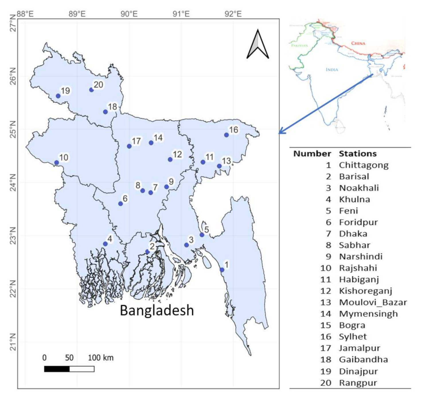
2.1. Study Area

The focus of this study was to investigate the impact of variabilities in the climate on crop yields. In Bangladesh (23.6850° N, 90.3563° E), 48.4% of the population is employed in agriculture, 70.1% of the land is devoted to agriculture, and agriculture accounts for 17.5% of the GDP [41]. Tea (Camellia Sinensis) was selected for the yield investigation study as it is susceptible to variables in the climate [7]. To achieve a good harvest of tea, very-specific conditions must be met. Crop yields are directly correlated to rainfall, humidity, and specific temperature [42]. As a South Asian country with a tropical monsoon climate, Bangladesh receives significant rainfall and has a perfect climate for growing tea during the monsoon season. Since 2008, the tea yield of Bangladesh has not increased compared to other nations, which is illustrated in Figure 1. An investigation of the reasons for this and a quantification of the tea yield is therefore essential.

Considering the above factors, investigating the impact of climate variability on tea yields in Bangladesh is well-suited for predicting agricultural crop yields. Interestingly, 96% of the annual tea production comes from the greater Sylhet area, 63% of which is contributed by the Moulvibazar district within the Sylhet division [25]. Bangladesh lies within the Indo-Gangetic plains of Southeast Asia in a complex delta with rich fertile soil. Three significant rivers (the Ganges, the Meghna, and the Brahmaputra), starting from the Himalayas, flow through the region into the Bay of Bengal. The country is subtropical, with a wet and humid climate [25]. On average, Bangladesh experiences about 1500 mm to 5000 mm of rainfall annually, with temperature and humidity in the range of 12–30 °C and 65–95%, respectively. In this study we have considered 20 stations in Bangladesh as illustrated in Figure 2. There are 150 tea estates in Sylhet, where most of the tea is produced in Bangladesh. This area is highly suitable due to the hilly nature of the landmass and an elevation in the range of 55 to 335 m. Water stress adversely affects the crop. A specific elevation is required for a greater crop yield as it reduces waterlogging due to heavy rainfall. This suits tea cultivation, which requires an average rainfall of 1000 mm per year. The plants also require a temperature range of 13–25 °C, which is within the temperature range seen throughout Bangladesh [19].

2.2. Satellite and Crop Data

Remote sensing was used to obtain satellite data on climate variability from Clouds and the Earth’s Radiant Energy System (CERES) and Modern-Era Retrospective analysis for Research and Applications, Version 2 (MERRA-2). MEERA-2 integrates satellite data with weather observations and models them as a continuous dataset in time and space. This modeling was conducted by the Goddard Earth Observing System, Version 5 (GEOS-5) [43]. The real-time weather observations were taken from the GOES satellite on a 5-kilometer image of the earth. The GEOS model and GOES satellite uses infrared energy to measure the amount of cloud cover. The model runs at 28 km/pixel to study the relation between weather and climate (GEOS-5: a high-resolution global atmospheric model, 2010). The satellite data from these two systems were used to gather specific data on the climate variables that affect yield in tea production. MEERA-2 provided temperature, humidity, wind-speed, surface soil wetness, and precipitation (mm/day) data. CERES provided data on the percentage of cloud and irradiance (W/m²). Historical data from the Foos and Agricultural Organization of the United Nations (FAO) were used for crop yield. FAOSTAT provides accessible data on crops from 245 countries from 1961. Using this extensive data from FAOSTAT, the tea production and crop yield of Bangladesh were modeled.

3. Materials and Methods

3.1. Theoretical Frameworks

This section summarizes the objective model (i.e., RF) and related algorithms (i.e., DR) used in this research study. The technical details of multivariate adaptive regressive splines (MARS) [44,45], extreme learning machine (ELM) [46,47], kernel ridge regression [48], and extreme gradient-boosting random forest (XGBRF) [49] are explained elsewhere.

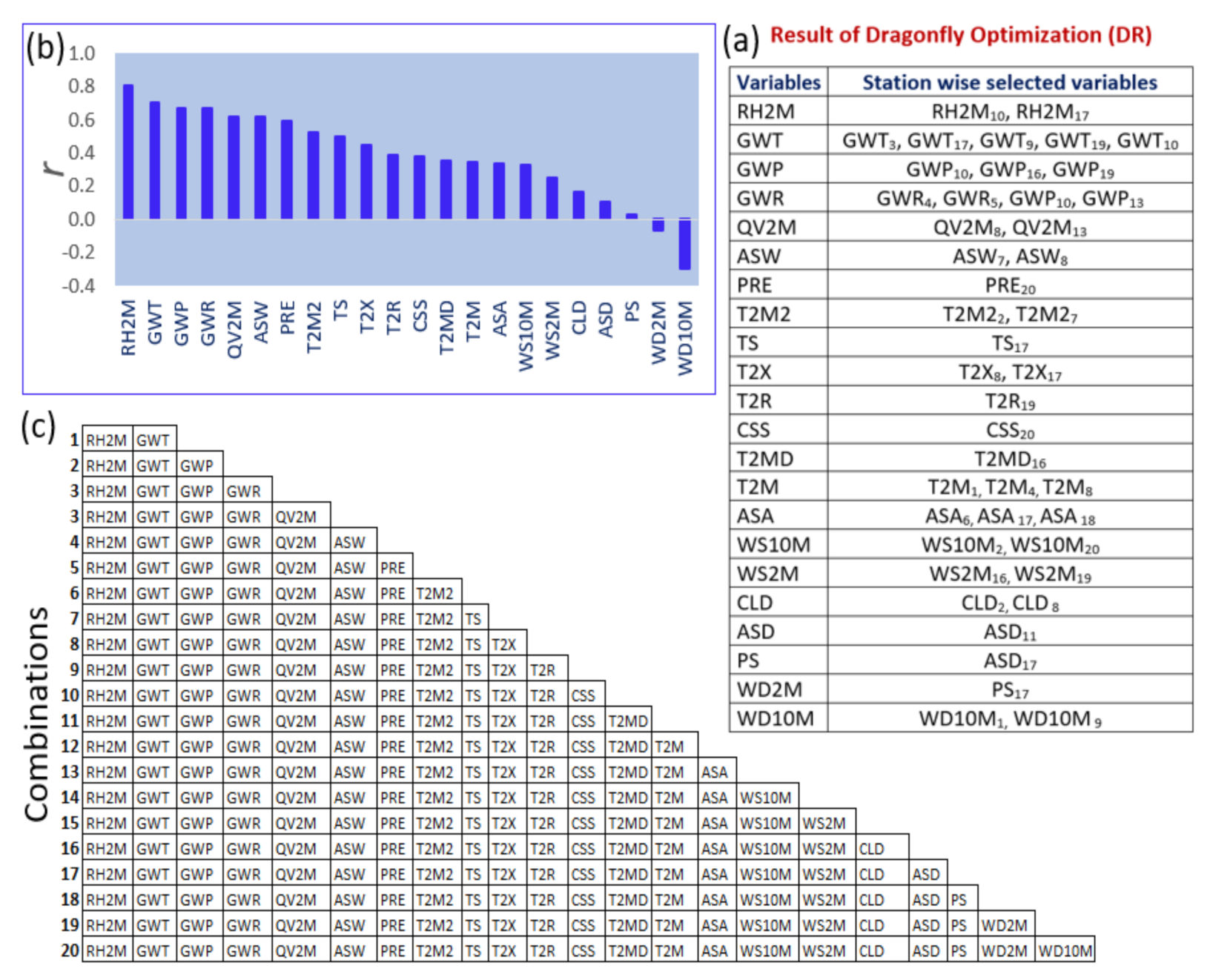
3.1.1. Dragonfly Optimization (DR)

The dragonfly algorithm (DR), proposed by Mirjalili [28], is a nature-inspired metaheuristic algorithm for solving optimization problems. Dragonflies, with 3000 different species, have two stages in their lifecycle, called nymph and adult [28,50]. The DR algorithm is mainly based on the hunting (called static swarm (feeding)) and migration mechanism of idealized dragonflies [31]. The dragonflies search for food sources over a small area by forming a small group of dragonflies in the hunting mechanism. The migration mechanism is characterized by a larger group of dragonflies flying with each other in one direction over a long distance so that the swarm migrates in a process. Five behaviors specify the actions of a dragonfly population: separation, alignment, cohesion, the behavior of foraging, and eluding enemies [51]. These behaviors are specified by the following equations:

1. Separation mechanism is characterized by avowing collisions with other neighbor individuals. This can be represented mathematically as:

$$S_i=-{\displaystyle \sum }_{j=1}^{N}X-X_j$$

(1)

where j ¼ 1; 2; …; N, i ¼ 1; 2;…; Np, N is the number of neighboring individuals, and Np is the number of population. X denotes the position of the current individual and X_j is the position of the jth neighboring individual. The velocity matching of individuals defines alignment to other neighboring search individuals, which is mathematically modeled as Equation (2):

$$A_{i }=\frac{{{\displaystyle \sum }}_{i=1}^N{V}_i}{N}$$

(2)

where V_j represents the jth neighborhood individual’s velocity and N is the neighborhood size. Cohesion specifies the tendency of individuals to move closer to each other or the neighborhood’s center of mass, which is mathematically represented as:

$$C_i=\frac{{{\displaystyle \sum }}_{j=1}^N{X}_j}{N}-X$$

(3)

where X is the current individual’s position, X_j specifies the jth neighboring individual of the X position, and N is the neighborhood size. Each individual survives through two key behaviors: attraction towards a food source, known as foraging, and escaping from enemies. The foraging behavior can be mathematically modeled as:

$$F_i=X^{+}-X$$

(4)

where $X^{+}$ represents the position of the food source and X represents the current individual’s position. The behavior of escaping from enemies can be represented as:

$$E_{i }=X^{-}+X$$

(5)

where $X^{-}$ represents the enemy’s position and X represents the current individual’s position. Step vector and position vector are used for solving optimization problems. Step vector can be mathematically represented as:

$$∆X_{t+1}=\left(s{S}_i+\alpha A_i+c{C}_i+f{F}_i+e{E}_i\right)+w∆X_t$$

(6)

where s represents the separation weight, S_i shows the separation of the ith individual, α is the alignment weight, A_i is the alignment of ith individual, c indicates the cohesion weight, C_i is the cohesion of the ith individual, f specifies the food factor, F_i symbolizes the food source of the ith individual, e is the enemy factor, E_i is the position of an enemy of the ith individual, w is the inertia weight, and t is the iteration number. The position vector can be represented as:

$$X^{t+1}=X^t+∆X^{t+1}$$

(7)

In the case of no adjacent individuals, the position vector is defined as:

$$X^{t+1}=Levy\left(d\right)\times X^t+X^t$$

(8)

where d is the dimension of the dragonfly individual.

The Levy flight strategy can be mathematically modeled as:

$$Levy\left(x\right)=0.01\times \frac{r_1\times \sigma }{{\left|r_2\right|}^{\frac{1}{\beta }}}$$

(9)

where $r_1$ and $r_2$ are the two stochastic numbers in (0,1) and β is a constant.

3.1.2. Random Forest (RF)

The random forest model is a popular supervised machine-learning algorithm developed by Breiman [52]. The RF model accumulates tree predictors associated with different values of random vectors sampled independently. In the training phase, a random forest model constructs decor-related decision trees, and the overall model output is obtained by averaging the output values of all the individual trees. The learner bagging algorithm is adopted in the random forest model for training any single tree [52]. The bootstrap samples of the training sets are repeatedly selected, and Gini impurity fits $t_b$ trees in these samples. Equation (10) calculates the predicted values for unseen complexes:

$$y=\frac{1}{B} {\displaystyle \sum }_{b=1}^B{t}_b\left(x\right)$$

(10)

The RF model obtains a better prediction result by modeling multiple trees instead of just one [53]. This methodology produces results with more accuracy than CART.

The overall RF model can be defined as:

(1)

Assemble $n_{trees}$ of bootstrapping, involving input predictors where n is the number of trees.

(2)

Develop an unpruned regression tree through randomization of input predictor samples for obtaining optimum split.

(3)

The tea yield is predicted from the aggregated prediction values from $n_{trees}$.

3.1.3. Support Vector Regression (S)

This research used support vector regression to select the spatiotemporal feature of the data. In his paper, Vapnik [53] developed the support vector regression (SVR) referred to as S. SVR can find the correlation between the input and output of a system from existing samples [54]. Using the following equation, the correlation is measured to predict the outputs from the inputs [55]:

$$f\left(x\right)=\omega \phi \left(x\right)+b$$

(11)

where $x$ represents the input vector, $\omega$ represents the weight vector of the input vector, and $\phi \left(x\right)$ is the kernel function (a nonlinear transfer function that transforms the input data to the higher dimensions) [55]. The Polynomial Kernel Function, Sigmoid Kernel Function, and Radial Basis Kernel Function (RBF) are a few popular kernel functions [56].

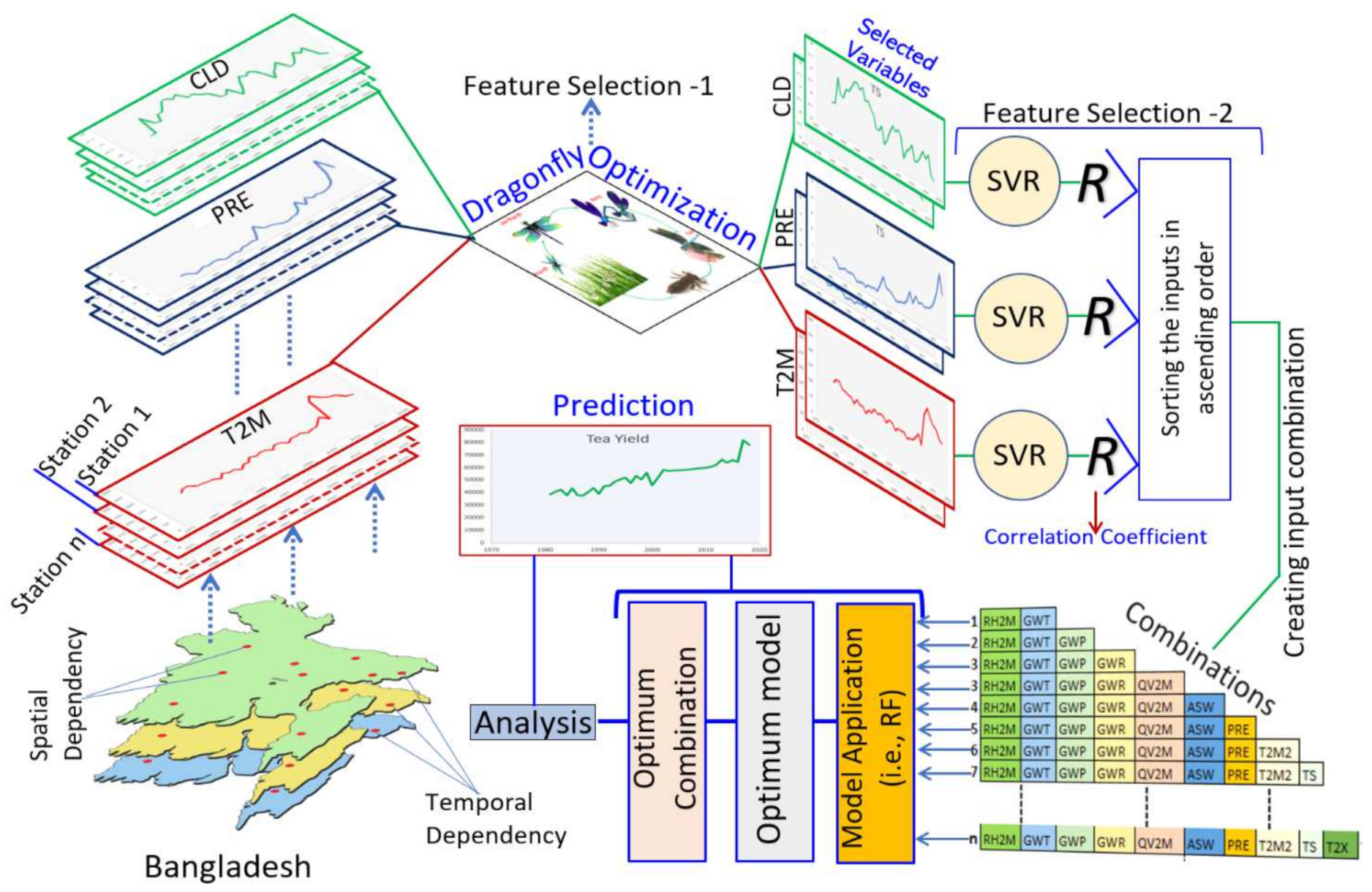
3.2. Development of DRS–RF Model

This research developed a hybrid machine-learning method (i.e., DRS–RF) coupled with dragonfly optimization algorithm and support vector regression using satellite-derived predictors to predict the tea yield of Bangladesh. The DRS–RF model was created on a PC with a 3.6 GHz Intel i7 processor and 16 GB of RAM. The proposed framework used the Python-based machine-learning library scikit-learn [57,58] to develop the RF and other benchmark models. The dragonfly algorithm was performed by MATLAB R2020b, and matplotlib [59] and QGIS tools were used for visualization. An integrated workflow of the present study to develop DRS–RF integrated with DR and support vector regression for tea yield prediction is shown in Figure 3. The development procedure of the hybrid DRS–RF model involved the following steps.

3.2.1. Feature Selection

The 22 variables from 20 stations of Bangladesh were collected from the MERRA-2 model to address the prediction problem of tea yield. The list of all predictor variables is tabulated in

Table 1. A description of the 22 predictors from the MERRA-2 satellite system used to design the hybrid DRS–RF model.

Acronyms	Description of Predictor Variables (Unit)
PS	Surface Pressure (kPa)
TS	Earth Skin Temperature (C)
T2M	Temperature at 2 Meters (C)
QV2M	Specific Humidity at 2 Meters (g/kg)
RH2M	Relative Humidity at 2 Meters (%)
WD2M	Wind Direction at 2 Meters (Degrees)
WS2M	Wind Speed at 2 Meters (m/s)
WD10M	Wind Direction at 10 Meters (Degrees)
WS10M	Wind Speed at 10 Meters (m/s)
T2MD	Dew/Frost Point at 2 Meters (C)
GWT	Surface Soil Wetness (1)
T2X	Temperature at 2 Meters Maximum (C)
T2M2	Temperature at 2 Meters Minimum (C)
GWP	Profile Soil Moisture (1)
GWR	Root Zone Soil Wetness (1)
CLD	Cloud Amount (%)
T2R	Temperature at 2 Meters Range (C)
PRE	Precipitation Corrected (mm/day)
ASA	All Sky Surface Albedo (Dimensionless)
ASW	All Sky Surface Longwave Downward Irradiance (W/m^2)
ASD	All Sky Surface Shortwave Downward Irradiance (MJ/m^2/day)
CSS	Clear Sky Surface PAR Total (W/m^2)

. Each variable of 20 stations was then run for the dragonfly optimization (DR) algorithm to select the significant variables from every station. Figure 4a shows the features selected by DR along with the respective stations (subscripted). After that, the study used support vector regression (S) as a feature selection approach in the 2nd step. The machine-learning approach is prevalent in selecting input variables [60]. The result of SVR is shown in Figure 4b, which shows that RH2M had the highest correlation coefficient (r), where WD10M showed the lowest. Based on the result of SVR shown in Figure 4b, the study constructed different combinations of predictors, adding them one by one in ascending order, as illustrated in Figure 4c. Because of the use of DR, the best-selected predictors were used for model application. With 100 iterations, the optimal number of dragonflies for the DR was fixed at 12.

3.2.2. Data Preparation

The screened variables from 20 stations were normalized to overcome the oversaturation problems of the model. The study normalized the following equations to ensure they received proportional attention in network training between (0,1) [45,61,62].

$${\mathsf{\Delta }}_{norm}=\frac{\mathsf{\Delta }-{\mathsf{\Delta }}_{min}}{{\mathsf{\Delta }}_{max}-{\mathsf{\Delta }}_{min}}$$

(12)

In Equation (12), $\mathsf{\Delta }$ is the respective variable, ${\mathsf{\Delta }}_{min}$ is the minimum variable, ${\mathsf{\Delta }}_{max}$ is the maximum, and ${\mathsf{\Delta }}_{norm}$ is the normalized variable. After normalizing the variables, the datasets were partitioned, 85% into training and 15% into testing; additionally, 15% of training datasets were kept for validation. The data partitioning was carried out by the trial-and-error method.

3.2.3. Model Application

Finally, the study developed the RF model to use the predictors’ data to predict the tea yield of Bangladesh. GridSearchCV was used to create an optimal architecture of the RF model (ccp_alpha = 0.1; min_impurity_decrease = 0.1; min_samples_leaf = 1; min_samples_split = 3; n_estimators = 200; random_state = 1). The performance of the proposed model was compared to that of standalone machine-learning models. Figure 3 shows the methodological steps of the proposed DRS–RF model.

3.2.4. Model Evaluation

Pearson’s Correlation Coefficient (r), root mean square error, and normalized root mean square error was used to assess the proposed machine-learning model (DRS–RF) and the benchmark models. Due to the geographical and climatological differences between the study stations, the study used relative RMSE (RRMSE) to compare tea yield. The following are the performance metrics, expressed in mathematical terms.

Correlation coefficient:

$$\left(r\right)={\left\{\frac{{{\displaystyle \sum }}_{i=1}^N\left(Y_{obs}-{\overline{Y}}_{obs}\right)\left(Y_{pred}-{\overline{Y}}_{pred}\right)}{\sqrt{{{\displaystyle \sum }}_{i=1}^N{\left(Y_{obs}-{\overline{Y}}_{obs}\right)}^2 {{\displaystyle \sum }}_{i=1}^N{\left(Y_{pred}-{\overline{Y}}_{pred}\right)}^2}}\right\}}^2$$

(13)

Relative Root Mean Square Error:

$$(\mathrm{RRMSE}, \%)=\frac{\sqrt{\frac{1}{N}{{\displaystyle \sum }}_{\mathrm{i}=1}^{\mathrm{N}}{\left(Y_{pred}-Y_{obs}\right)}^2}}{\frac{1}{N}{{\displaystyle \sum }}_{i=1}^N(Y_{obs})} \times 100$$

(14)

Mean Absolute Percentage Error:

$$\left(\mathrm{MAPE};\%\right)=\frac{1}{\mathrm{N}} \left({\displaystyle \sum }_N^{\mathrm{i}=1}\left|\frac{ ({\mathrm{Y}}_{pred}-Y_{obs})}{Y_{obs}} \right|\right)*100$$

(15)

In Equations (13)–(15), $Y_{obs}$ and $Y_{pred}$ represent the observed and predicted wheat yield values for ith test value; ${\overline{Y}}_{obs}$ and ${\overline{Y}}_{pred}$ refer to their average wheat yield, respectively; and N is defined as the number of observations (years).

4. Results

For predicting tea yield (Y) in Bangladesh, this study developed and tested a hybrid RF predictive model called BRS–RF, coupled with the dragonfly optimization algorithm (DR) and support vector regression (S) for feature selection to improve performance accuracy. The model was evaluated using statistical score metrics (Equations (13)–(15)) and diagnostic plots of both the observed and predicted Y for each dataset.

Table 2. Evaluation of hybrid DRS–RF vs. benchmark modes concerning different combinations, as specified in Figure 4. The correlation coefficient (r) and mean absolute percentage error (MAPE, %).

Combinations	KRR		MARS		ELM		RF		SVR		XGBRF
	R	MAPE	R	MAPE	R	MAPE	R	MAPE	R	MAPE	R	MAPE
	Standalone Approach
	0.897	21.36	0.390	20.90	0.387	33.78	0.763	14.86	0.955	21.72	0.945	20.79
Hybrid Approach (Using Dragonfly Optimization and SVR, DRS)
1	0.947	20.47	0.885	22.14	0.442	19.82	0.981	14.84	0.335	18.69	0.869	19.37
2	0.921	22.00	0.895	20.36	0.888	8.29	0.951	15.05	0.712	18.79	0.853	20.40
3	0.909	21.97	0.868	19.87	0.406	10.43	0.987	14.95	0.801	19.30	0.961	19.71
4	0.877	21.43	0.868	19.87	0.395	19.78	0.958	14.90	0.723	19.14	0.951	20.04
5	0.871	21.84	0.868	19.87	0.455	19.56	0.959	14.91	0.671	21.74	0.961	20.19
6	0.865	21.79	0.817	22.03	0.814	25.96	0.965	14.87	0.685	21.83	0.957	20.14
7	0.880	21.85	0.817	22.03	0.922	26.57	0.993	11.95	0.699	21.71	0.857	20.49
8	0.889	21.93	0.817	22.03	0.783	36.92	0.942	14.94	0.679	21.45	0.964	20.36
9	0.884	21.89	0.790	21.53	0.884	22.18	0.965	14.87	0.815	20.41	0.951	20.72
10	0.875	22.14	0.790	21.53	0.536	18.52	0.984	14.91	0.550	20.38	0.954	20.34
11	0.872	22.08	0.790	21.53	0.855	18.20	0.886	14.83	0.560	20.30	0.972	19.84
12	0.893	22.14	0.790	21.53	0.926	28.97	0.963	14.98	0.745	20.22	0.867	20.61
13	0.903	22.21	0.790	21.53	0.588	12.46	0.937	14.84	0.368	19.62	0.975	19.76
14	0.908	22.91	0.351	29.97	0.367	13.59	0.958	14.94	0.817	16.46	0.977	19.63
15	0.904	23.04	0.351	29.97	0.695	21.40	0.942	14.69	0.936	21.16	0.965	19.82
16	0.889	22.82	0.307	43.58	0.491	31.51	0.928	14.76	0.928	21.71	0.974	20.22
17	0.883	22.42	0.167	53.18	0.196	38.48	0.990	14.98	0.915	20.34	0.975	20.23
18	0.909	22.52	0.075	28.27	0.286	51.26	0.872	14.68	0.938	20.38	0.970	20.06
19	0.909	22.44	0.075	28.27	0.370	44.25	0.929	14.76	0.935	20.45	0.915	20.03
20	0.898	22.27	0.075	28.27	0.361	27.09	0.961	14.83	0.927	21.11	0.977	20.23
21	0.894	22.33	0.678	29.32	0.438	45.67	0.981	14.94	0.929	21.13	0.971	20.09

compares the observed and predicted Y for the testing data in terms of r and MAPE for different combinations and their respective standalone models. The input combinations prepared by dragonfly optimization and support vector regression were improved by our proposed DRS–RF model. The objective hybrid DRS–RF model obtained the highest r (0.993) and the lowest MAPE (11.95%) with combination 7, followed by the DRS–XGBRF model with combination 14. The DRS–KRR model with combination 1 included RH2M and GWT, which improved the performance (r = 0.947; MAPE = 20.47). The standalone model of RF showed poor performance; the hybrid machine-learning predictive model outperformed the other models using satellite-derived hydro-meteorological variables.

Figure 5 shows the results of an in-depth investigation of the correlation coefficient (r) and MAPE (%), which demonstrated that the proposed hybrid DRS–RF model performed significantly better than other models in predicting Y for the loop of 20 combinations. The r-value and MAPE (%) were distributed between the lower quartile (25th percentile) and the upper quartile (75th percentile). However, one outlier was discovered to be greater than the 25th percentile in terms of the r-value. In contrast, the MAPE showed a very condensed distribution, resulting in an improved performance in predicting the Y value with the RF model coupled with Dragonfly Optimization and support vector regression. The standalone models showed lower r-values, with Figure 5 indicating that the proposed hybrid machine-learning predictive model outperformed various competing methods.

To better understand the predictive performance of the proposed hybrid DRS–RF model, the study employed the RRMSE (%) value for the standalone models (i.e., KRR, MARS, ELM, RF, SVR, and XGBRF) and their respective hybrid models, along with the percent change of RRMSE (%) while applied to the proposed hybrid approach (i.e., DRS–RF). Figure 6 shows that the newly constructed DRS–RF model had the lowest RRMSE (18%), significantly improving the performance of the standalone RF model (12%). The standalone ELM model had the highest RRMSE (%) value (30%), and the lowest value was found for the RF model (29%). After analyzing the different combinations with the proposed hybrid models and several benchmark models, the proposed hybrid model produced significantly superior results to standalone machine-learning modeling when it came to Y predicting.

As shown in Figure 7, a scatterplot of the observed and predicted Y using the DRS–RF and standalone RF models indicated a precise prediction as an additional evaluation of the hybrid predictive model (i.e., DRS–RF). The scatter plots show that the coefficient of determination (R²) was related to the goodness-of-fit between the predicted and observed Y as well as a line of least-square fitting with the appropriate equation: Y = mx + c, where “m” is the gradient and “c” is the regression line’s y-intercept. As shown in Figure 7, the suggested model outperformed the baseline model by a wide margin, with an R² value that was significantly higher using a hybrid machine-learning model (i.e., DRS–RF). The magnitudes reported from the hybrid DRS–RF model were the closest to unity when measured in pairs (m|R²), with values of 0.986|0.07 (m|R²) in comparison to the RF model (0.582|0.06). The unity for the other models (i.e., DRS–KRR, DRS–MARS, and DRS–SVR) provided a lower value of R². The newly proposed hybrid RF predictive model outperformed the benchmark models using a carefully selected set of satellite-based predictor variables.

Figure 8 depicts the study site; the empirical cumulative distribution function (ECDF) examined the plots of various prediction skills in terms of the empirical cumulative distribution function (ECDF). The study plotted the normalized absolute prediction error (PE) in this figure. The generated error ranged from 0 to 0.25 within the 90th percentile when the proposed hybrid RF model was compared to the benchmark models, demonstrating that the DRS–RF model combined with dragonfly optimization and support vector regression performed the best. However, the ECDF plot for the other benchmark models showed poor distribution, comparatively.

5. Discussion

The inclusion of remote sensing (RS) satellite data, MERRA- 2 and CERES-syn1 data of climate variables, and tea yield data were significant in this study to assess their suitability for tea yield forecast. Twenty-two climate variables were individually tested before additional variables were added to test climatic conditions for tea production. Out of the 22 parameters tested, 10 parameters were significant for forecasting. Relative and specific humidity, surface soil wetness, root zone soil moisture, all-sky surface longwave downward irradiance, precipitation, the temperature at 2 m, and the earth skin temperature were shown to be essential factors for tea production in the study.

The proposed DRS–RF model generated spatial and temporal dependency, outperforming other standalone or hybrid models in tea yield prediction. The study considered 20 stations in Bangladesh and found suitable climatic conditions in Sylhet. RS data can be cost-effective, providing almost real-time information for tea and other crops [2,7,63,64,65]. RS data can sometimes act poorly due to the spectral mixing issue for the same greenery and shrubs in an exact location [66], and newer satellites such as Sentinel-2 with a return cycle of five days instead of 13–16 days and 13 high-resolution spectral bands can radically change the crop-monitoring and -predicting procedures [67]. The results show that combining climate and satellite data achieved the best performance using our proposed hybrid DRS–RF model to provide an accurate forecast for tea yield prediction. The proposed DRS–RF model provided the highest correlation coefficient (r) (0.933) and the lowest mean absolute error (MAPE) (11.95%) compared to all other tested standalone models (RF, KRR, MARS, ELM, RF, SVR, and XGBRF) and their respective hybrid models (Table 2). Out of the twenty-two variables first tested individually and then integrated one by one, combination 7 was revealed as achieving the best performance (Figure 4c). The water-supply-related variables such as relative humidity, soil moisture, and precipitation proved to be significant factors for tea yield, which agrees with previous studies [2,67,68]. The same studies also confirm the highest correlation coefficient using climate variables.

Additionally, this study explored the use of the RS satellite dataset and combined it with advanced machine algorithms to predict tea yield, as studies have previously explored with other crops [2]. In the future, further tea yield forecasting can be carried out incorporating deep-learning approaches [69,70,71] and including more features such as the elevation of the land [72] and vegetation indices, as described in [73]. The present study is important for developing countries such as Bangladesh, with land and climates suitable for producing cash crops such as tea. This carries more importance when tea is used for export purposes after satisfying the national demand. The analysis also suggested suitable locations where tea is not currently being produced, which essentially agreed with the findings of Saha et al. [6] and could be used to increase tea cultivation.

6. Conclusions

In Bangladesh, almost half of the total population is directly or indirectly dependent on agriculture, and most of the land is arable. Remote sensing data is imperative to modernize agriculture and provide farmers and policymakers with near-real-time information on climate variables to make an informed decision. This helps ensure better returns, minimize production cost losses, and improve seed yield and overall production. The novel hybrid random forest (RF) model was combined with dragonfly optimization for the first feature selection and support vector regression for the second feature selection to find the optimum combination with the DRS–RF model. The overall findings of the study can be summarized as follows:

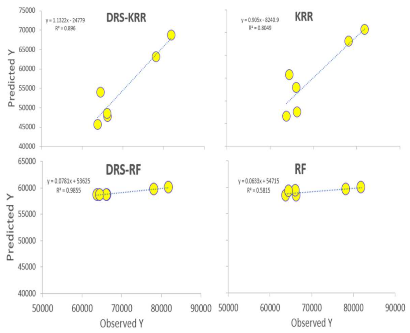
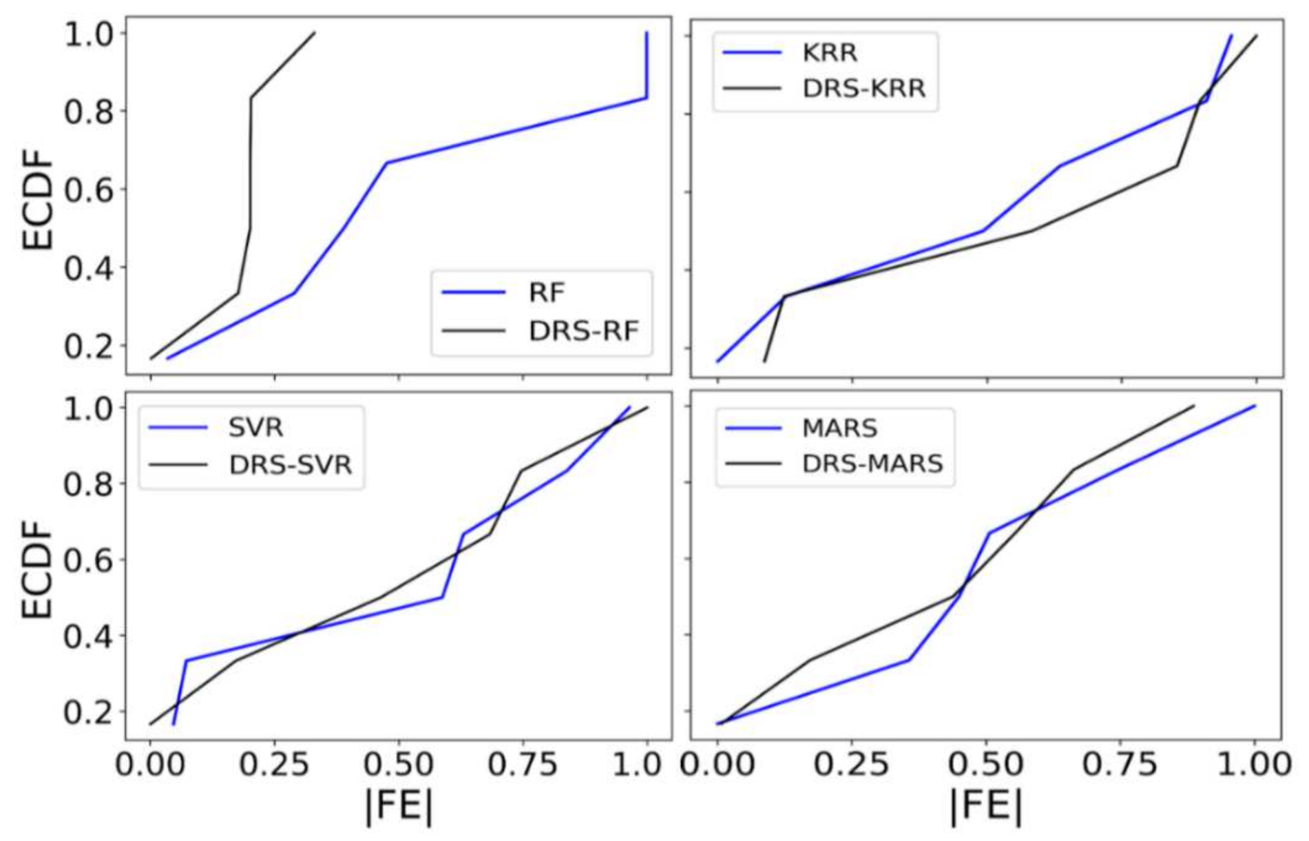
• The proposed hybrid DRS–RF model showed the best performance in predicting the tea yield by a significant margin.
• The DRS–RF model showed the highest correlation coefficient (r) (0.933) and the lowest mean absolute percentage error (MAPE) (11.95%) with combination 7, out of 20 combinations of hydro-meteorological variables.
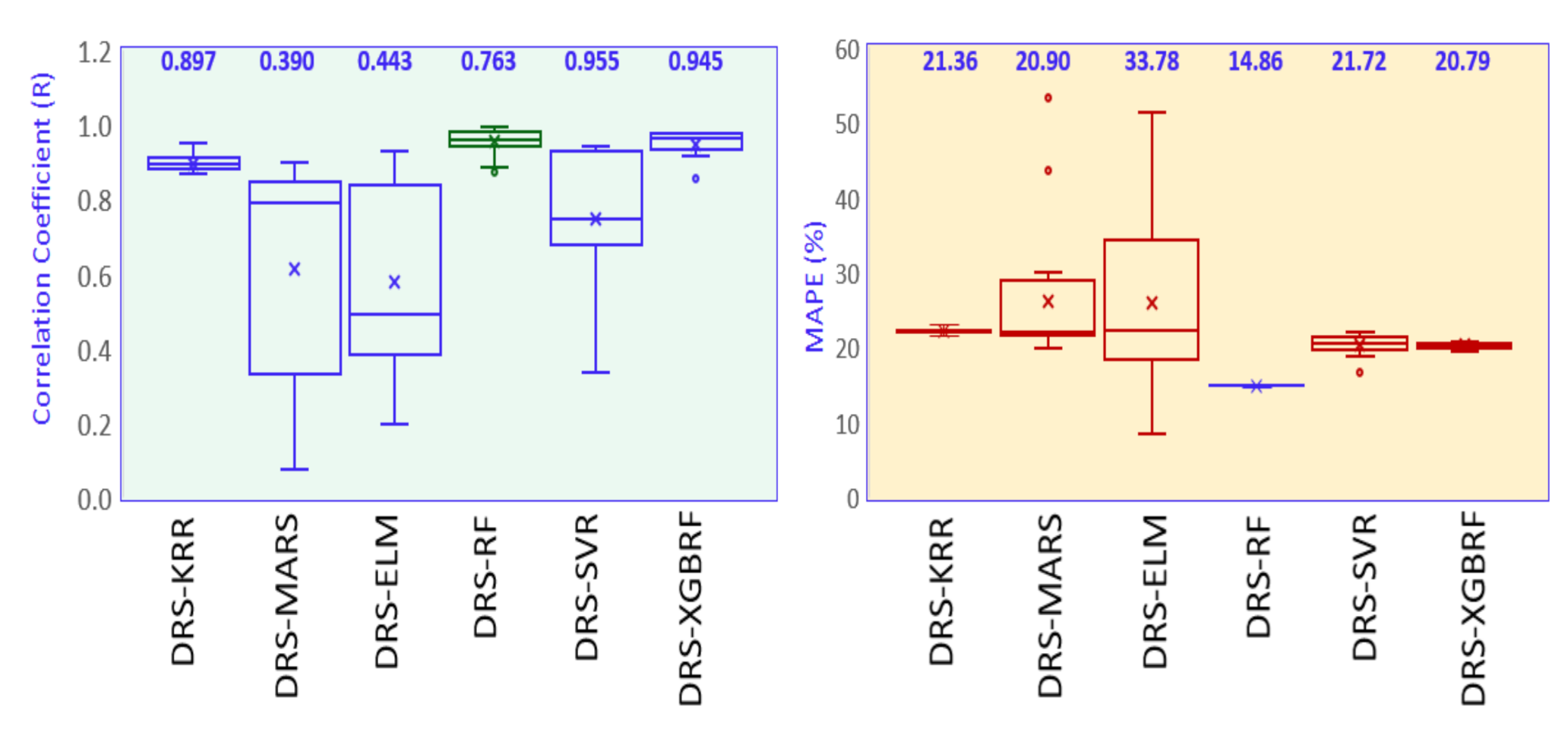
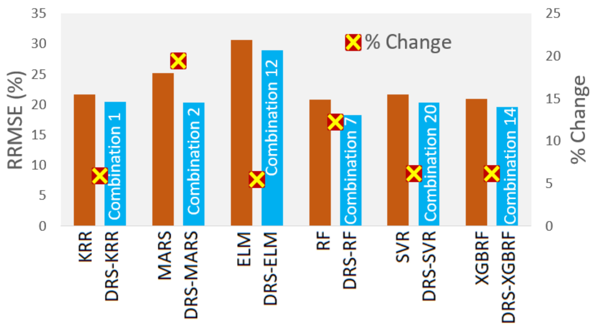
• The study also checked the standalone models RF, KRR, MARS, ELM, RF, SVR, and XGBRF and their respective hybrid models. The hybrid DRS–KRR and hybrid DRS–XGBRF models (which preferred combination 14) demonstrated significant performances with combination 1, with an r value of 0.947 and an MAPE of 20.47. The proposed model also showed the lowest relative root mean square error (RRMSE; 18%), whereas standalone Extreme Learning Machines (ELM) had an RRMSE value of 30%, followed by RF at 29%.
• The proposed model could be used for other crops with feature selection approaches in future works. Numerous authors have suggested that a popular and widely used deep-learning methodology could also be involved at the modeling stage [7,45,61,62]. Lastly, the model could be tested at several temporal horizons to give more accurate predictions for other geographies.

In a nutshell, using remote sensing data, the proposed hybrid model could be applied to numerous national and global problems, such as carbon emission and climate studies, to name a few, helping governments and policymakers reach economic, financial, and social sustainability.

References

1. Statista. Global Tea Consumption 2012–2025. Available online: https://www.statista.com/statistics/940102/global-tea-consumption/ (accessed on 30 December 2021).
2. Cai, Y.; Guan, K.; Lobell, D.; Potgieter, A.B.; Wang, S.; Peng, J.; Xu, T.; Asseng, S.; Zhang, Y.; You, L. Integrating satellite and climate data to predict wheat yield in Australia using machine learning approaches. Agric. For. Meteorol. 2019, 274, 144–159. [Google Scholar] [CrossRef]
3. Islam, M.A.; Sumy, M.S.A.; Uddin, M.A.; Hossain, M.S. Fitting ARIMA model and forecasting for the tea production, and internal consumption of tea (per year) and export of tea. Int. J. Mater. Math. Sci. 2020, 2, 8–15. [Google Scholar]
4. Kamruzzaman, M.; Parveen, S.; Das, A.C. Livelihood improvement of tea garden workers: A scenario of marginalized women group in Bangladesh. Asian J. Agric. Ext. Econ. Sociol. 2015, 7, 1–7. [Google Scholar] [CrossRef]
5. Islam, G.; Iqbal, M.; Quddus, K.; Ali, M. Present status and future needs of tea industry in Bangladesh. Proc.-Pak. Acad. Sci. 2005, 42, 305. [Google Scholar]
6. Saha, J.; Adnan, K.M.; Sarker, S.A.; Bunerjee, S. Analysis of growth trends in area, production and yield of tea in Bangladesh. J. Agric. Food Res. 2021, 4, 100136. [Google Scholar] [CrossRef]
7. Ahmed, A.; Deo, R.C.; Raj, N.; Ghahramani, A.; Feng, Q.; Yin, Z.; Yang, L. Deep Learning Forecasts of Soil Moisture: Convolutional Neural Network and Gated Recurrent Unit Models Coupled with Satellite-Derived MODIS, Observations and Synoptic-Scale Climate Index Data. Remote Sens. 2021, 13, 554. [Google Scholar] [CrossRef]
8. Cheserek, B.C.; Elbehri, A.; Bore, J. Analysis of links between climate variables and tea production in the recent past in Kenya. Donnish J. Res. Environ. Stud. 2015, 2, 5–17. [Google Scholar]
9. Mosleh, M.K.; Hassan, Q.K.; Chowdhury, E.H. Application of remote sensors in mapping rice area and forecasting its production: A review. Sensors 2015, 15, 769–791. [Google Scholar] [CrossRef] [Green Version]
10. Prasad, A.K.; Chai, L.; Singh, R.P.; Kafatos, M. Crop yield estimation model for Iowa using remote sensing and surface parameters. Int. J. Appl. Earth Obs. Geoinf. 2006, 8, 26–33. [Google Scholar] [CrossRef]
11. Noureldin, N.; Aboelghar, M.; Saudy, H.; Ali, A. Rice yield forecasting models using satellite imagery in Egypt. Egypt. J. Remote Sens. Space Sci. 2013, 16, 125–131. [Google Scholar] [CrossRef] [Green Version]
12. Aday, S.; Aday, M.S. Impact of COVID-19 on the food supply chain. Food Qual. Saf. 2020, 4, 167–180. [Google Scholar] [CrossRef]
13. Seleiman, M.F.; Selim, S.; Alhammad, B.A.; Alharbi, B.M.; Juliatti, F.C. Will novel coronavirus (COVID-19) pandemic impact agriculture, food security and animal sectors? Biosci. J. 2020, 36, 1315–1326. [Google Scholar] [CrossRef]
14. Meenken, E.; Wheeler, D.; Brown, H.; Teixeira, E.; Espig, M.; Bryant, J.; Triggs, C. Framework for uncertainty evaluation and estimation in deterministic agricultural models. In Nutrient Management in Farmed Landscapes; Occasional Report; Massey University: Palmerston North, New Zealand, 2020. [Google Scholar]
15. Kingsley, J.; Afu, S.M.; Isong, I.A.; Chapman, P.A.; Kebonye, N.M.; Ayito, E.O. Estimation of soil organic carbon distribution by geostatistical and deterministic interpolation methods: A case study of the southeastern soils of nigeria. Environ. Eng. Manag. J. 2021, 20, 1077–1085. [Google Scholar] [CrossRef]
16. Holman, I.; Tascone, D.; Hess, T. A comparison of stochastic and deterministic downscaling methods for modelling potential groundwater recharge under climate change in East Anglia, UK: Implications for groundwater resource management. Hydrogeol. J. 2009, 17, 1629–1641. [Google Scholar] [CrossRef]
17. Sharma, E.; Deo, R.C.; Prasad, R.; Parisi, A.V. A hybrid air quality early-warning framework: An hourly forecasting model with online sequential extreme learning machines and empirical mode decomposition algorithms. Sci. Total Environ. 2020, 709, 135934. [Google Scholar] [CrossRef]
18. Sharma, E.; Deo, R.C.; Prasad, R.; Parisi, A.V.; Raj, N. Deep Air Quality Forecasts: Suspended Particulate Matter Modeling With Convolutional Neural and Long Short-Term Memory Networks. IEEE Access 2020, 8, 209503–209516. [Google Scholar] [CrossRef]
19. Das, A.C.; Noguchi, R.; Ahamed, T. Integrating an Expert System, GIS, and Satellite Remote Sensing to Evaluate Land Suitability for Sustainable Tea Production in Bangladesh. Remote Sens. 2020, 12, 4136. [Google Scholar] [CrossRef]
20. Rama Rao, N.; Kapoor, M.; Sharma, N.; Venkateswarlu, K. Yield prediction and waterlogging assessment for tea plantation land using satellite image-based techniques. Int. J. Remote Sens. 2007, 28, 1561–1576. [Google Scholar] [CrossRef]
21. Schwalbert, R.A.; Amado, T.; Corassa, G.; Pott, L.P.; Prasad, P.V.; Ciampitti, I.A. Satellite-based soybean yield forecast: Integrating machine learning and weather data for improving crop yield prediction in southern Brazil. Agric. For. Meteorol. 2020, 284, 107886. [Google Scholar] [CrossRef]
22. Peng, B.; Guan, K.; Zhou, W.; Jiang, C.; Frankenberg, C.; Sun, Y.; He, L.; Köhler, P. Assessing the benefit of satellite-based solar-induced chlorophyll fluorescence in crop yield prediction. Int. J. Appl. Earth Obs. Geoinf. 2020, 90, 102126. [Google Scholar] [CrossRef]
23. Rajapakse, R.; Tripathi, N.K.; Honda, K. Modelling tea (Camellia (L) O. kuntze) yield using satellite derived LAI, land use and meteorological data. In Proceedings of the 21st Asian Conference on Remote Sensing ACRS 2000, Taipei, Taiwan, 4–8 December 2000. [Google Scholar]
24. Feng, Y.; Peng, Y.; Cui, N.; Gong, D.; Zhang, K. Modeling reference evapotranspiration using extreme learning machine and generalized regression neural network only with temperature data. Comput. Electron. Agric. 2017, 136, 71–78. [Google Scholar] [CrossRef]
25. Rahman, A. Modeling of Tea Production in Bangladesh Using Autoregressive Integrated Moving Average (ARIMA) Model. J. Appl. Comput. Math. 2017, 6, 349. [Google Scholar] [CrossRef] [Green Version]
26. Hossain, M.; Abdulla, F. Forecasting the tea production of Bangladesh: Application of ARIMA model. Jordan J. Math. Stat. 2015, 8, 257–270. [Google Scholar]
27. Li, J.; Cheng, K.; Wang, S.; Morstatter, F.; Trevino, R.P.; Tang, J.; Liu, H. Feature selection: A data perspective. ACM Comput. Surv. 2017, 50, 1–45. [Google Scholar] [CrossRef]
28. Mirjalili, S. Dragonfly algorithm: A new meta-heuristic optimization technique for solving single-objective, discrete, and multi-objective problems. Neural Comput. Appl. 2016, 27, 1053–1073. [Google Scholar] [CrossRef]
29. Cui, X.; Li, Y.; Fan, J.; Wang, T.; Zheng, Y. A hybrid improved dragonfly algorithm for feature selection. IEEE Access 2020, 8, 155619–155629. [Google Scholar] [CrossRef]
30. Too, J.; Mirjalili, S. A hyper learning binary dragonfly algorithm for feature selection: A COVID-19 case study. Knowl.-Based Syst. 2021, 212, 106553. [Google Scholar] [CrossRef]
31. Hammouri, A.I.; Mafarja, M.; Al-Betar, M.A.; Awadallah, M.A.; Abu-Doush, I. An improved dragonfly algorithm for feature selection. Knowl.-Based Syst. 2020, 203, 106131. [Google Scholar] [CrossRef]
32. Deo, R.C.; Kisi, O.; Singh, V.P. Drought forecasting in eastern Australia using multivariate adaptive regression spline, least square support vector machine and M5Tree model. Atmos. Res. 2017, 184, 149–175. [Google Scholar] [CrossRef] [Green Version]
33. Lazri, M.; Ameur, S. Combination of support vector machine, artificial neural network and random forest for improving the classification of convective and stratiform rain using spectral features of SEVIRI data. Atmos. Res. 2018, 203, 118–129. [Google Scholar] [CrossRef]
34. Roodposhti, M.S.; Safarrad, T.; Shahabi, H. Drought sensitivity mapping using two one-class support vector machine algorithms. Atmos. Res. 2017, 193, 73–82. [Google Scholar] [CrossRef]
35. Tripathi, S.; Srinivas, V.V.; Nanjundiah, R.S. Downscaling of precipitation for climate change scenarios: A support vector machine approach. J. Hydrol. 2006, 330, 621–640. [Google Scholar] [CrossRef]
36. Devak, M.; Dhanya, C.; Gosain, A. Dynamic coupling of support vector machine and K-nearest neighbour for downscaling daily rainfall. J. Hydrol. 2015, 525, 286–301. [Google Scholar] [CrossRef]
37. Li, W.; Yang, M.; Liang, Z.; Zhu, Y.; Mao, W.; Shi, J.; Chen, Y. Assessment for surface water quality in Lake Taihu Tiaoxi River Basin China based on support vector machine. Stoch. Environ. Res. Risk Assess. 2013, 27, 1861–1870. [Google Scholar] [CrossRef]
38. Shi, Y.; Song, L.; Xia, Z.; Lin, Y.; Myneni, R.B.; Choi, S.; Wang, L.; Ni, X.; Lao, C.; Yang, F. Mapping annual precipitation across mainland China in the period 2001–2010 from TRMM3B43 product using spatial downscaling approach. Remote Sens. 2015, 7, 5849–5878. [Google Scholar] [CrossRef] [Green Version]
39. Pour, S.H.; Shahid, S.; Chung, E.-S.; Wang, X.-J. Model output statistics downscaling using support vector machine for the projection of spatial and temporal changes in rainfall of Bangladesh. Atmos. Res. 2018, 213, 149–162. [Google Scholar] [CrossRef]
40. Deka, P.C. Support vector machine applications in the field of hydrology: A review. Appl. Soft Comput. 2014, 19, 372–386. [Google Scholar]
41. Food and Agriculture Organization of the United Nations. Available online: https://www.fao.org/home/en/ (accessed on 29 December 2021).
42. Wijeratne, M. Vulnerability of Sri Lanka tea production to global climate change. Water Air Soil Pollut. 1996, 92, 87–94. [Google Scholar] [CrossRef]
43. Reichle, R.H.; Liu, Q.; Koster, R.D.; Draper, C.S.; Mahanama, S.P.; Partyka, G.S. Land surface precipitation in MERRA-2. J. Clim. 2017, 30, 1643–1664. [Google Scholar] [CrossRef]
44. Ghali, U.M.; Usman, A.; Degm, M.A.A.; Alsharksi, A.N.; Naibi, A.M.; Abba, S. Applications of artificial intelligence-based models and multi-linear regression for the prediction of thyroid stimulating hormone level in the human body. Int. J. Adv. Sci. Technol. 2020, 29, 3690–3699. [Google Scholar]
45. Ahmed, A.M.; Deo, R.C.; Feng, Q.; Ghahramani, A.; Raj, N.; Yin, Z.; Yang, L. Deep learning hybrid model with Boruta-Random forest optimiser algorithm for streamflow forecasting with climate mode indices, rainfall, and periodicity. J. Hydrol. 2021, 599, 126350. [Google Scholar] [CrossRef]
46. Şahin, M. Comparison of modelling ANN and ELM to estimate solar radiation over Turkey using NOAA satellite data. Int. J. Remote Sens. 2013, 34, 7508–7533. [Google Scholar] [CrossRef]
47. Heddam, S. Use of Optimally Pruned Extreme Learning Machine (OP-ELM) in Forecasting Dissolved Oxygen Concentration (DO) Several Hours in Advance: A Case Study from the Klamath River, Oregon, USA. Environ. Processes 2016, 3, 909–937. [Google Scholar] [CrossRef]
48. Naik, J.; Satapathy, P.; Dash, P. Short-term wind speed and wind power prediction using hybrid empirical mode decomposition and kernel ridge regression. Appl. Soft Comput. 2018, 70, 1167–1188. [Google Scholar] [CrossRef]
49. Zhang, W.; Wu, C.; Zhong, H.; Li, Y.; Wang, L. Prediction of undrained shear strength using extreme gradient boosting and random forest based on Bayesian optimization. Geosci. Front. 2021, 12, 469–477. [Google Scholar] [CrossRef]
50. Jafari, M.; Chaleshtari, M.H.B. Using dragonfly algorithm for optimization of orthotropic infinite plates with a quasi-triangular cut-out. Eur. J. Mech.-A/Solids 2017, 66, 1–14. [Google Scholar] [CrossRef]
51. Li, L.-L.; Zhao, X.; Tseng, M.-L.; Tan, R.R. Short-term wind power forecasting based on support vector machine with improved dragonfly algorithm. J. Clean. Prod. 2020, 242, 118447. [Google Scholar] [CrossRef]
52. Breiman, L. Random Forests. Mach. Learn. 2001, 45, 5–32. [Google Scholar] [CrossRef] [Green Version]
53. Tso, G.K.F.; Yau, K.K.W. Predicting electricity energy consumption: A comparison of regression analysis, decision tree and neural networks. Energy 2007, 32, 1761–1768. [Google Scholar] [CrossRef]
54. Vapnik, V. The Nature of Statistical Learning Theory; Springer: New York, NY, USA, 1995; Volume 2, p. 209. [Google Scholar]
55. Dodangeh, E.; Panahi, M.; Rezaie, F.; Lee, S.; Bui, D.T.; Lee, C.-W.; Pradhan, B. Novel hybrid intelligence models for flood-susceptibility prediction: Meta optimization of the GMDH and SVR models with the genetic algorithm and harmony search. J. Hydrol. 2020, 590, 125423. [Google Scholar] [CrossRef]
56. Ghimire, S.; Deo, R.C.; Raj, N.; Mi, J. Deep solar radiation forecasting with convolutional neural network and long short-term memory network algorithms. Appl. Energy 2019, 253, 113541. [Google Scholar] [CrossRef]
57. Kramer, O. Scikit-learn. In Machine Learning for Evolution Strategies; Springer: Cham, Switzerland, 2016; pp. 45–53. [Google Scholar] [CrossRef]
58. Pedregosa, F.; Varoquaux, G.; Gramfort, A.; Michel, V.; Thirion, B.; Grisel, O.; Blondel, M.; Prettenhofer, P.; Weiss, R.; Dubourg, V. Scikit-learn: Machine learning in Python. J. Mach. Learn. Res. 2011, 12, 2825–2830. [Google Scholar]
59. Barrett, P.; Hunter, J.; Miller, J.T.; Hsu, J.-C.; Greenfield, P. Matplotlib—A Portable Python Plotting Package. In Proceedings of the Astronomical Data Analysis Software and Systems XIV, Pasadena, CA, USA, 24–27 October 2004; Volume 347, p. 91. [Google Scholar]
60. Ranković, V.; Radulović, J.; Radojević, I.; Ostojić, A.; Čomić, L. Neural network modeling of dissolved oxygen in the Gruža reservoir, Serbia. Ecol. Model. 2010, 221, 1239–1244. [Google Scholar] [CrossRef]
61. Ahmed, A.A.M.; Deo, R.C.; Feng, Q.; Ghahramani, A.; Raj, N.; Yin, Z.; Yang, L. Hybrid deep learning method for a week-ahead evapotranspiration forecasting. Stoch. Environ. Res. Risk Assess. 2021, 1–19. [Google Scholar] [CrossRef]
62. Ahmed, A.M.; Deo, R.C.; Ghahramani, A.; Raj, N.; Feng, Q.; Yin, Z.; Yang, L. LSTM integrated with Boruta-random forest optimiser for soil moisture estimation under RCP4. 5 and RCP8. 5 global warming scenarios. Stoch. Environ. Res. Risk Assess. 2021, 35, 1851–1881. [Google Scholar] [CrossRef]
63. Doraiswamy, P.C.; Moulin, S.; Cook, P.W.; Stern, A. Crop yield assessment from remote sensing. Photogramm. Eng. Remote Sens. 2003, 69, 665–674. [Google Scholar] [CrossRef]
64. Anderson, M.C.; Norman, J.M.; Mecikalski, J.R.; Otkin, J.A.; Kustas, W.P. A climatological study of evapotranspiration and moisture stress across the continental United States based on thermal remote sensing: 2. Surface moisture climatology. J. Geophys. Res. Atmos. 2007, 112, 1–13. [Google Scholar] [CrossRef]
65. Teng, W.; de Jeu, R.; Doraiswamy, P.; Kempler, S.; Mladenova, I.; Shannon, H. Improving world agricultural supply and demand estimates by integrating NASA remote sensing soil moisture data into USDA world agricultural outlook board decision making environment. In Proceedings of the American Society of Photogrammetry and Remote Sensing 2010 Annual Conference, San Diego, CA, USA, 26–30 April 2010. [Google Scholar]
66. Dihkan, M.; Guneroglu, N.; Karsli, F.; Guneroglu, A. Remote sensing of tea plantations using an SVM classifier and pattern-based accuracy assessment technique. Int. J. Remote Sens. 2013, 34, 8549–8565. [Google Scholar] [CrossRef]
67. Zhao, Y.; Potgieter, A.B.; Zhang, M.; Wu, B.; Hammer, G.L. Predicting wheat yield at the field scale by combining high-resolution Sentinel-2 satellite imagery and crop modelling. Remote Sens. 2020, 12, 1024. [Google Scholar] [CrossRef] [Green Version]
68. Landau, S.; Mitchell, R.; Barnett, V.; Colls, J.; Craigon, J.; Payne, R. A parsimonious, multiple-regression model of wheat yield response to environment. Agric. For. Meteorol. 2000, 101, 151–166. [Google Scholar] [CrossRef]
69. Elavarasan, D.; Vincent, P.D. Crop yield prediction using deep reinforcement learning model for sustainable agrarian applications. IEEE Access 2020, 8, 86886–86901. [Google Scholar] [CrossRef]
70. Wang, A.X.; Tran, C.; Desai, N.; Lobell, D.; Ermon, S. Deep transfer learning for crop yield prediction with remote sensing data. In Proceedings of the 1st ACM SIGCAS Conference on Computing and Sustainable Societies; Menlo Park/San Jose, CA, USA, 20–22 June 2018, pp. 1–5. [CrossRef]
71. Khaki, S.; Wang, L. Crop yield prediction using deep neural networks. Front. Plant Sci. 2019, 10, 621. [Google Scholar] [CrossRef] [PubMed] [Green Version]
72. Das, A.C.; Noguchi, R.; Ahamed, T. An Assessment of Drought Stress in Tea Estates Using Optical and Thermal Remote Sensing. Remote Sens. 2021, 13, 2730. [Google Scholar] [CrossRef]
73. Wójtowicz, M.; Wójtowicz, A.; Piekarczyk, J. Application of remote sensing methods in agriculture. Commun. Biometry Crop Sci. 2016, 11, 31–50. [Google Scholar]
Figure 1. A comparison of tea yield between 2008 and 2018 over the neighboring countries of Bangladesh.
Remotesensing 14 00805 g001
Figure 2. The study area and selected 20 stations which were used to extract the predictor variables to develop the hybrid DRS–RF model.
Remotesensing 14 00805 g002
Figure 3. An integrated workflow of the present study to develop DRS–RF integrated with DR and support vector regression for tea yield prediction.
Remotesensing 14 00805 g003
Figure 4. (a) The selected predictors with their respective stations (subscripted) using a butterfly optimization algorithm; (b) correlation coefficient (r) of the SVR model for feature selection; (c) the input combinations prepared by selecting the best resulting variables one-by-one in ascending order.
Remotesensing 14 00805 g004
Figure 5. Box plots of proposed hybrid models (i.e., DRS–RF) along with their respective standalone counterparts in predicting tea yield in terms of Correlation Coefficient (r) and MAPE (%).
Remotesensing 14 00805 g005
Figure 6. The RRMSE of the proposed model and other comparison models and the respective change in percentage from the standalone model.
Remotesensing 14 00805 g006
Figure 7. Scatter plot of predicted vs. observed Y using the proposed hybrid model and comparison models. A least-square regression line and coefficient of determination (R2) with a linear fit equation are shown in each subpanel.
Remotesensing 14 00805 g007
Figure 8. Empirical Cumulative Distribution Function (CDF) of prediction error |FE| of Y generated by the proposed DRS–RF vs. benchmark models.
Remotesensing 14 00805 g008