Article

DGS-SLAM: A Fast and Robust RGBD SLAM in Dynamic Environments Combined by Geometric and Semantic Information

1
School of Geodesy and Geomatics, Wuhan University, Wuhan 430079, China
2
School of Geomatics Science and Technology, Nanjing Tech University, Nanjing 211800, China
*
Author to whom correspondence should be addressed.
Remote Sens. 2022, 14(3), 795; https://doi.org/10.3390/rs14030795
Submission received: 27 December 2021 / Revised: 28 January 2022 / Accepted: 1 February 2022 / Published: 8 February 2022

Abstract

:
Visual Simultaneous Localization and Mapping (VSLAM) is a prerequisite for robots to accomplish fully autonomous movement and exploration in unknown environments. At present, many impressive VSLAM systems have emerged, but most of them rely on the static world assumption, which limits their application in real dynamic scenarios. To improve the robustness and efficiency of the system in dynamic environments, this paper proposes a dynamic RGBD SLAM based on a combination of geometric and semantic information (DGS-SLAM). First, a dynamic object detection module based on the multinomial residual model is proposed, which executes the motion segmentation of the scene by combining the motion residual information of adjacent frames and the potential motion information of the semantic segmentation module. Second, a camera pose tracking strategy using feature point classification results is designed to achieve robust system tracking. Finally, according to the results of dynamic segmentation and camera tracking, a semantic segmentation module based on a semantic frame selection strategy is designed for extracting potential moving targets in the scene. Extensive evaluation in public TUM and Bonn datasets demonstrates that DGS-SLAM has higher robustness and speed than state-of-the-art dynamic RGB-D SLAM systems in dynamic scenes.

Graphical Abstract

1. Introduction

Simultaneous localization and mapping (SLAM) [1] is a crucial technology to achieve the autonomous perception of intelligent robots for applications such as augmented reality, indoor navigation, and autonomous vehicles [2,3,4]. It enables the robot’s positional estimation and scene construction in unknown environments by analyzing its onboard sensors. Visual SLAM [5] uses the camera as the primary sensor, which has the advantages of low cost, easy installation, and rich environmental information. Due to the increasing amount of attention from scholars in the past few decades, many VSLAM systems with good performance have been developed, such as LSD-SLAM [6], DSO [7], and ORB-SLAM2 [8].
Although existing VSLAM systems have achieved successful performance in some cases, there are still some problems to be solved. For example, most VSLAM algorithms rely heavily on the static world assumption. In this assumption, the environment is static, and the change of field of view only comes from the camera’s motion, which limits its applicability in the real world. Dynamic objects such as moving people, animals, and vehicles will lead to many incorrect data associations, which will further have severe negative impacts on pose estimation and scene construction. The effect of dynamic feature points can be reduced using methods such as bundle adjustment (BA) [8] or Random Sample Consensus (RANSAC) [9]. However, the static area must account for most of the scene, which is not necessarily satisfied in the real world. For example, in crowded places, dynamic objects tend to occupy more areas, which will cause the algorithm to fail. Therefore, improving the robustness of visual SLAM algorithms in dynamic environments remains a considerable challenge.
The critical problem of dynamic SLAM is to segment dynamic objects in the environment and determine the correct data association. We classify dynamic SLAM solutions into two classes: geometry-based methods [10,11,12,13,14,15,16,17,18,19] and semantic-based methods [20,21,22,23,24,25,26,27,28,29,30,31]. Geometry-based approaches detect dynamic objects in a scene by constructing multiple sets of geometric constraints. However, they ignore the potential motility of the target, which leads to the missed detection of moving targets. Semantic-based approaches detect and remove dynamic targets from the environment by instance segmentation networks. Although such algorithms have good performance in dynamic target segmentation, there are two main problems. Most semantic-based dynamic SLAM algorithms perform instance segmentation for each frame, which consumes many computing resources and is not suitable for real-time and small robot applications. On the other hand, the instance segmentation network can only detect potential moving targets with prior knowledge and cannot judge their actual moving properties.
To address these issues, we extend the work of ORB-SLAM3 and propose a fast and robust dynamic RGB-D SLAM system (DGS-SLAM) based on the combination of geometric models and semantic information. The main contributions of this paper are summarized as follows:
  • A dynamic object detection algorithm is proposed to decrease the impact of dynamic objects on camera ego-motion estimation. It combines the geometric motion information of the current frame and the potential motion information of the historical semantic frames to adaptively segment of dynamic objects.
  • A semantic segmentation module based on the semantic frame selection strategy is designed. It can provide enough potential motion information when the scene and dynamic objects change, and it significantly reduces the computational cost of the system.
  • Extensive experiments are carried out on public TUM and Bonn datasets with state-of-the-art dynamic SLAM methods. The experimental results show that DGS-SLAM has competitive localization accuracy and runtime results.
The rest of this paper is organized as follows: Section 2 discusses related work. Section 3 introduces our proposed system in detail. Section 4 details the experimental process and comparative analysis of the experimental results. Section 5 discusses the experimental results. Finally, we conclude our work and present future research directions in Section 6.

2. Related Work

2.1. Visual SLAM

The main task of VSLAM is to solve the camera position and construct the scene graph by pixel matching of image sequences. After more than a decade of development, many practical open-source SLAM algorithms have emerged. MonoSLAM [32] uses the Extended Kalman Filter (EKF) [33] as the back-end to track sparse feature points on the front-end, but MonoSLAM has only a single thread and can only handle a limited number of sparse features. In the same year, Klein et al. proposed the first keyframe-based visual SLAM system PTAM [34]. PTAM proposed a dual-threaded architecture of tracking and mapping, which realized parallel processing of camera trajectory tracking and environment map construction. Meanwhile, bundle adjustment is used to obtain higher localization accuracy. The ORB-SLAM2 [8] system proposed by Mur Artal et al. is one of the most well-known SLAM systems. It extends the algorithm framework of PTAM and adds a loop closure thread on the basis of tracking and local mapping threads, which effectively reduces the cumulative error. ORB-SLAM2 improves and optimizes feature point extraction and keyframe selection, which has good operation efficiency and stability. Based on ORB-SLAM2, ORB-SLAM3 [35] tightly integrates visual and inertial information and adds a multiple map system (ATLAS [36]), which can work in real-time in various environments. However, these methods cannot distinguish between static and dynamic targets in the scene, which can cause VSLAM systems to degrade the accuracy of localization and map building due to incorrect data association. Therefore, further research is necessary to explore visual SLAM algorithms in dynamic environments.

2.2. Geometry-Based Dynamic SLAM

The main idea of geometry-based approaches is to use robust weighting functions or motion consistency constraints to reject outliers and improve localization accuracy. Kim et al. [17] eliminated outliers by estimating the nonparametric background model of depth scenes and realized camera motion estimation based on the background model. Li et al. [16] proposed a frame-to-keyframe edge-based RGB-D SLAM, which adds the static weights of the foreground edge points of the keyframe to the Intensity Assisted Iterative Closest Point method (IAICP) to calculate the current frame pose. Sun et al. [12] proposed an RGB-D-based online motion removal method. This method constructs and incrementally updates the foreground model and uses the optical flow method for tracking. In addition, they [19] extended their previous work by using optical flow to identify and remove dynamic feature points with RGB images as the only input. Staticfusion [15] realizes static background reconstruction by simultaneously estimating the camera motion as well as a probabilistic static segmentation. Dai et al. [14] proposed establishing Delaunay triangulation and comparing the changes of triangle edges in adjacent frames to determine the correlation of feature points to distinguish dynamic and static map points.
Geometry-based methods improve the performance of existing systems to a certain extent and often have a faster speed. However, they lack semantic information and cannot detect moving targets using prior knowledge of the scene. The robustness of geometry-based methods in dynamic scenes is often lower than that of semantic-based SLAM.

2.3. Semantic-Based Dynamic SLAM

Semantic-based dynamic SLAM methods use a deep learning network to segment the input image and obtain each target’s mask and semantic label. Then potential targets in the scene are removed based on the semantic information in a single image frame. To improve the stability of dynamic object recognition, most semantically-based dynamic SLAMs perform instance segmentation for each input frame. For example, DS-SLAM [29], based on ORB-SLAM2 and SegNet [37], uses polar line constraints to make motion consistency judgments on other semantic segmentation targets. This system only considers predefined dynamic objects, such as persons. DynaSLAM [30] combines Mask R-CNN [38] and multi-view geometry for dynamic object detection in the RGB-D data and implements background inpainting. However, its multi-view geometry algorithm suffers from the region growing algorithm, which takes much time to detect dynamic objects if there are many dynamic points in the scene. VDO-SLAM [31] jointly computes and optimizes camera pose, dynamic and static points, and pose of moving objects and uses dense optical flow to maximize the number of tracking points on moving objects. However, its need instance segmentation and optical flow tracking for each frame cause it to be processed only offline.
Some approaches use a keyframe-based semantic segmentation strategy to improve the algorithm’s operational efficiency. For example, Detect-SLAM [28] integrates ORB-SLAM2 with a single-shot multibox detector (SSD) [39] to make the two functions mutually beneficial. It detects only the moving objects in keyframes and performs moving probability propagation by feature matching in the tracking thread. RDS-SLAM [23] proposes a non-blocked model to update and propagate semantic information through moving probability, which can realize real-time tracking of dynamic scenes. Although these methods can achieve faster operation, they rely too much on the instance segmentation results of keyframes, and no corresponding semantic segmentation frame selection strategy is designed for the characteristics of dynamic environments.

3. Methods

An overview of DGS-SLAM, which is implemented based on the RGB-D mode of ORB-SLAM3, is illustrated in Figure 1. When a new frame is acquired, our system will start to complete the scene’s motion segmentation and camera ego-motion estimation. First, we use the dynamic object detection module to efficiently segment the motion objects in each frame based on the geometric motion information of the current frame and the potential motion information of the historical semantic frames. Second, the current frame pose is computed by an improved tracking module. After that, we input the current frame into the semantic segmentation module for judgment. If the semantic frame selection strategy is satisfied, the potential motion information in the semantic frames is extracted using a lightweight deep learning network. Finally, the back-end optimization and loop closing modules of ORB-SLAM3 are used to maintain the current map. Compared to the original ORB-SLAM3, we modified the tracking thread and added the following two modules:
1.
Dynamic object detection module: First, we compute the initial pose of the current frame using the coarse tracking algorithm. Second, we use the K-means algorithm to perform spatial clustering and then build a residual model of the clustering results. Finally, we combine the semantic information of the prior dynamic objects and the residual distribution of the current frame to calculate an adaptive threshold to complete the motion segmentation of the scene.
2.
Semantic segmentation module: The semantic segmentation module first makes a judgment on the input frames. If it is a semantic frame, instance segmentation is performed, and the semantic label and mask of the potential dynamic objects are input to the dynamic object detection module.
Figure 1. Overview of DGS-SLAM.
Remotesensing 14 00795 g001

3.1. Dynamic Object Detection Module

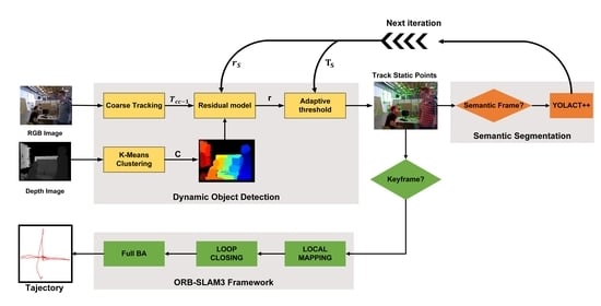
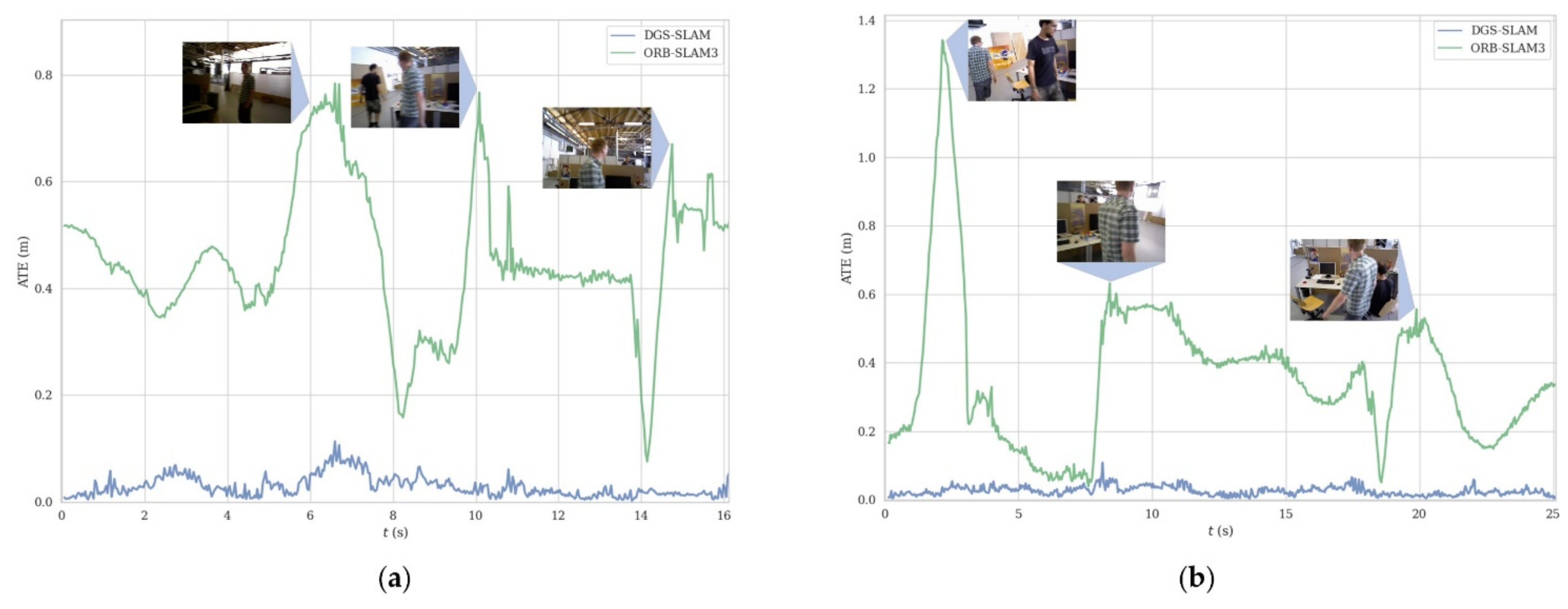
The instance segmentation network can detect motion objects labeled in the training set. However, relying only on semantic segmentation results will have two problems. On the one hand, some moving objects, such as balloons, tables, and chairs, are not priori dynamic objects and cannot be recognized by the semantic detection module. On the other hand, there are stationary cars or people in scenes with low dynamics. The semantic network cannot judge their real motion properties, leading to incorrect segmentation of dynamic objects, thus reducing the number of feature points and the localization accuracy. To this end, we design a dynamic object detection module by combining geometric motion information and potential motion information to achieve segmentation of dynamic objects in the scene.
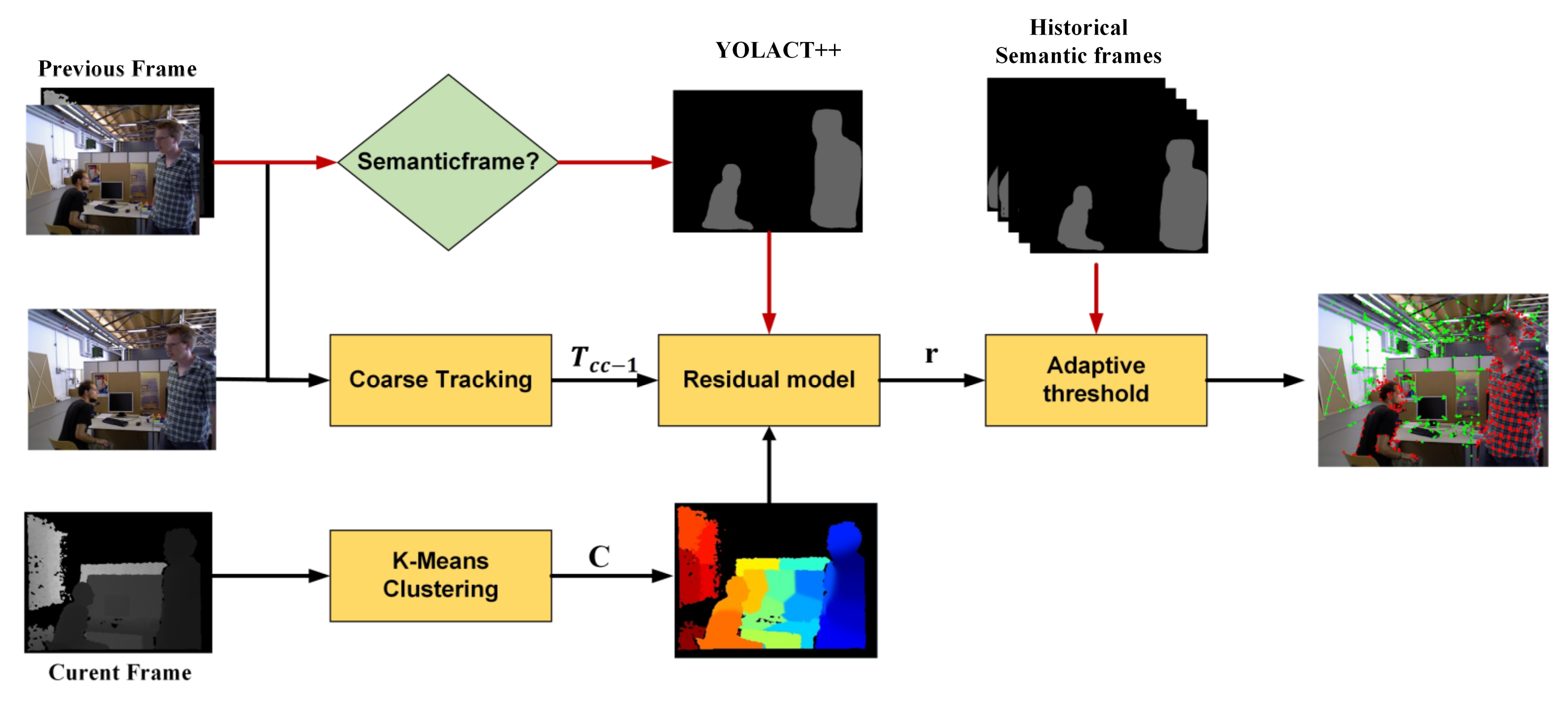
The flowchart of the dynamic object detection module is shown in 
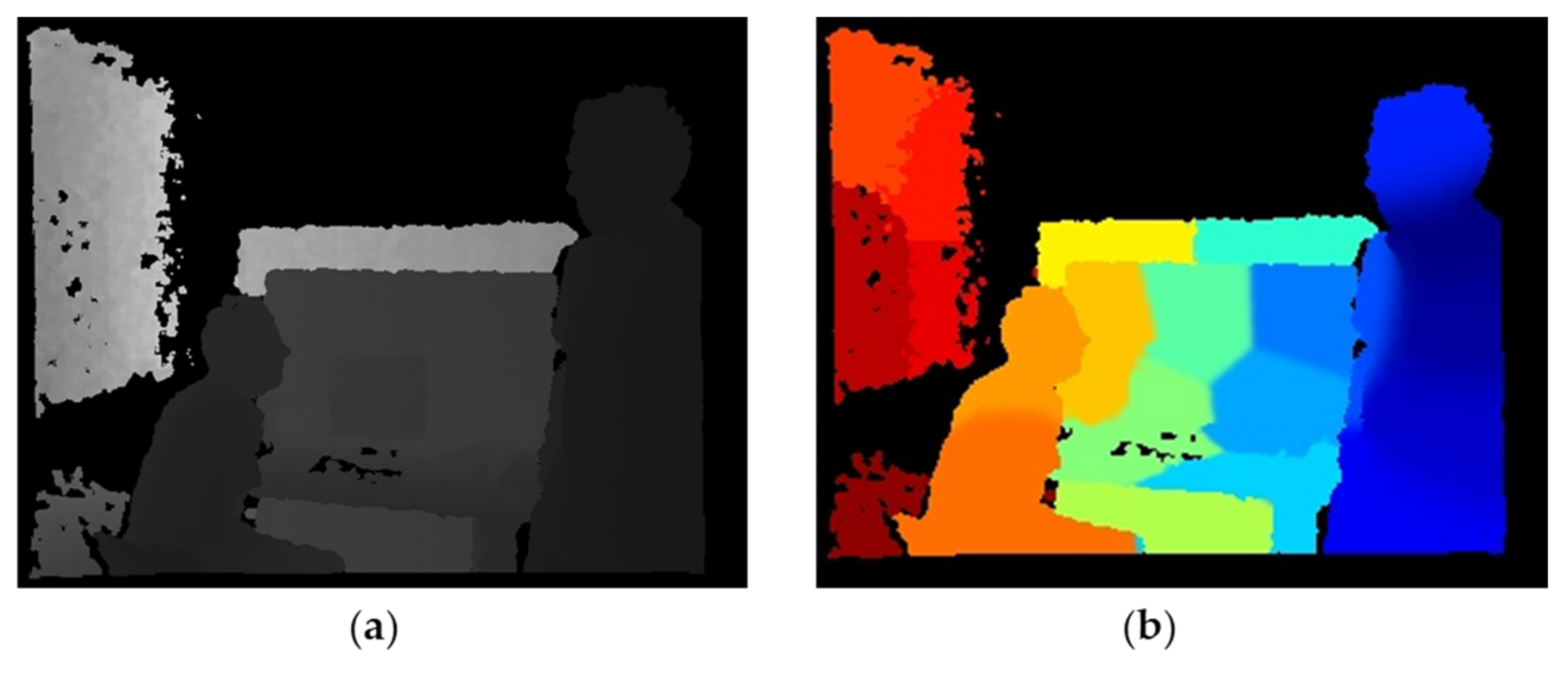
Figure 2. First, we use the depth and spatial information-based K-means clustering algorithm for clustering segmentation of depth images. The motion segmentation problem of image pixels can be transformed into the motion segmentation of clusters. Second, we calculate the initial pose of adjacent RGB images using coarse tracking. Then the residual model is built based on the initial pose of the camera, the spatial correlation of the clusters, and the continuity of the motion. Finally, the adaptive threshold is calculated based on the residual distribution of the current frame and the instance segmentation results of the historical semantic frames to realize the motion segmentation of the scene. The dynamic object detection module can not only integrate geometric and semantic information but also run alone without semantic information input.

3.1.1. Scene Clustering

Many current scene segmentation methods use pixel-wise segmentation. However, they lack the spatial correlation of the overall region, which easily generates noise and reduces the segmentation accuracy. Compared with pixel-wise segmentation, the spatial clustering approach has two advantages. On the one hand, each cluster can be viewed as a rigid body, thus transforming pixel-level non-rigid scenes into cluster-level rigid scenes. On the other hand, spatial clustering prevents false detection caused by single-point measurement noise and dramatically simplifies the complexity of motion segmentation. Therefore, we segment each new depth image into K clusters using the K-means algorithm, where points close to each other in 3D space are grouped together. First, we generate 3D point coordinates using depth values and inverse projection functions. Then K points are randomly selected as the center of mass of the initial clustering. By calculating the distance between each 3D spatial point and the cluster center, the belonging relationship is judged. Finally, several iterations are repeated until the position of the center point does not change, and the segmentation of the spatial scene is completed (Figure 3).

3.1.2. Residual Model

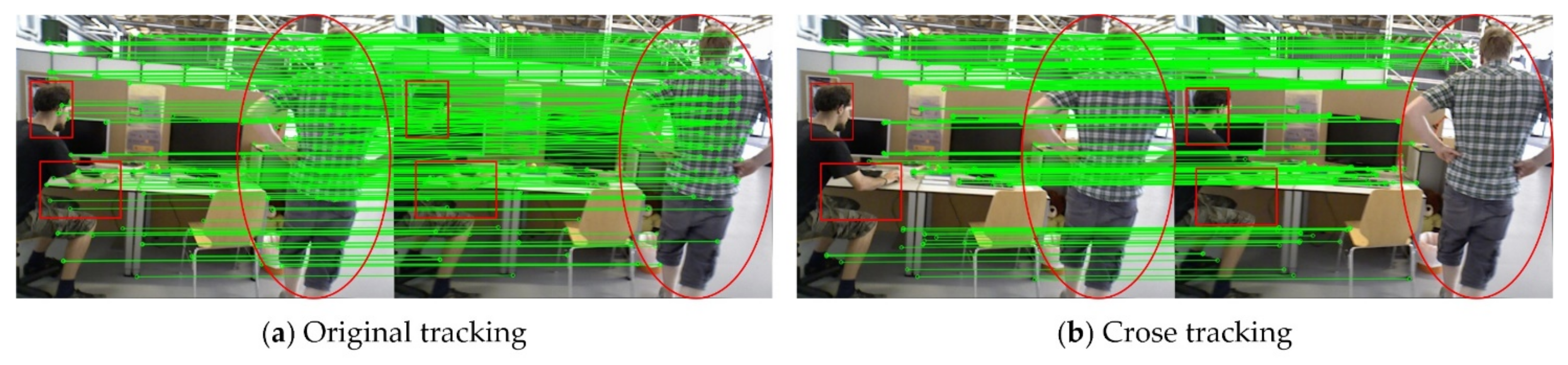
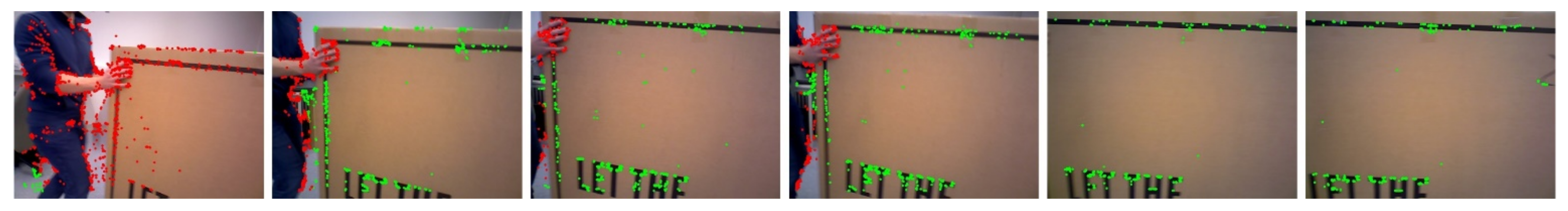
If the camera is stationary in dynamic scenes, the motion segmentation problem becomes very simple. However, the camera is often in motion, and the overall scene is clearly in motion, making it hard to identify dynamic objects directly. To achieve dynamic object detection, the initial pose of the current frame needs to be computed to determine which clusters follow the motion pattern of the camera and which clusters do not. Therefore, we perform coarse tracking of the system to calculate the initial pose of the current frame. According to the motion model, we project the static feature points in the previous frame to the current frame to find the matching points and minimize the reprojection error to optimize the initial pose T cc 1 . As shown in 
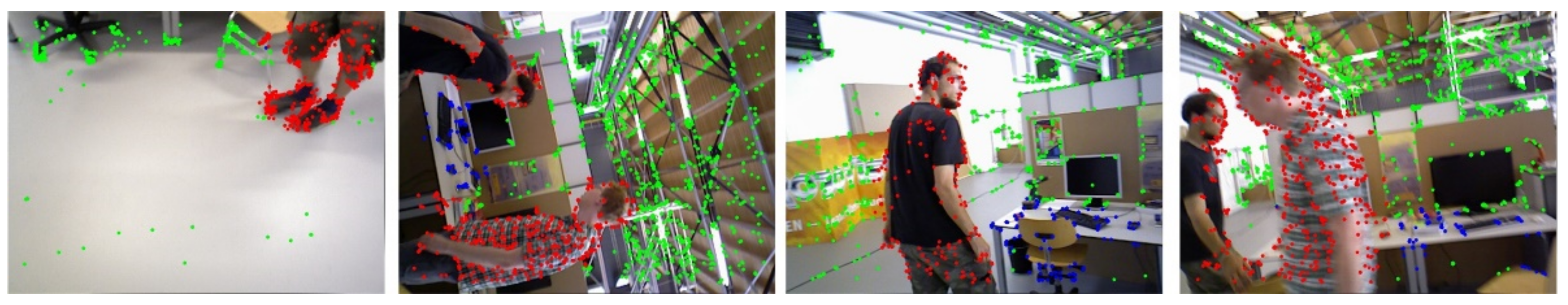
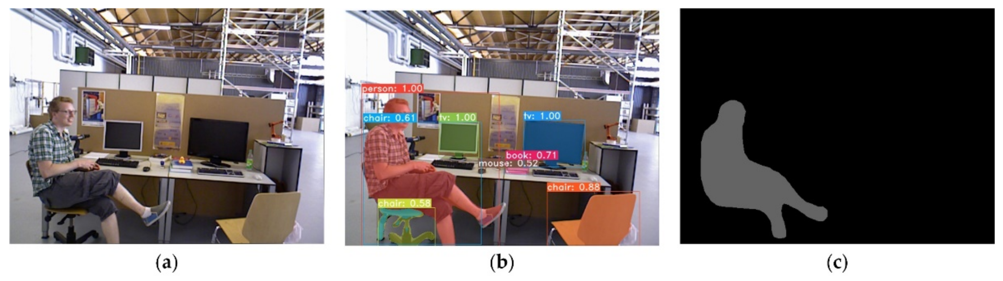
Figure 4, the original ORB matching establishes many incorrect correspondences on the human body, which provides unstable data association for camera tracking. In contrast, coarse tracking uses only the static feature points of the previous frame, which reduces the influence of dynamic objects on the positional computation and makes the initial positional T c c 1 with high accuracy, which is helpful for subsequent motion segmentation of the current frame.
To identify the dynamic and static parts of the scene, motion segmentation needs to be performed according to the residual of the cluster. Therefore, we established a residual model to calculate the residual of each cluster:
r = r D + r S + r P
where r D is the data residual, r S is the spatial residual, and r P is the priori residual.
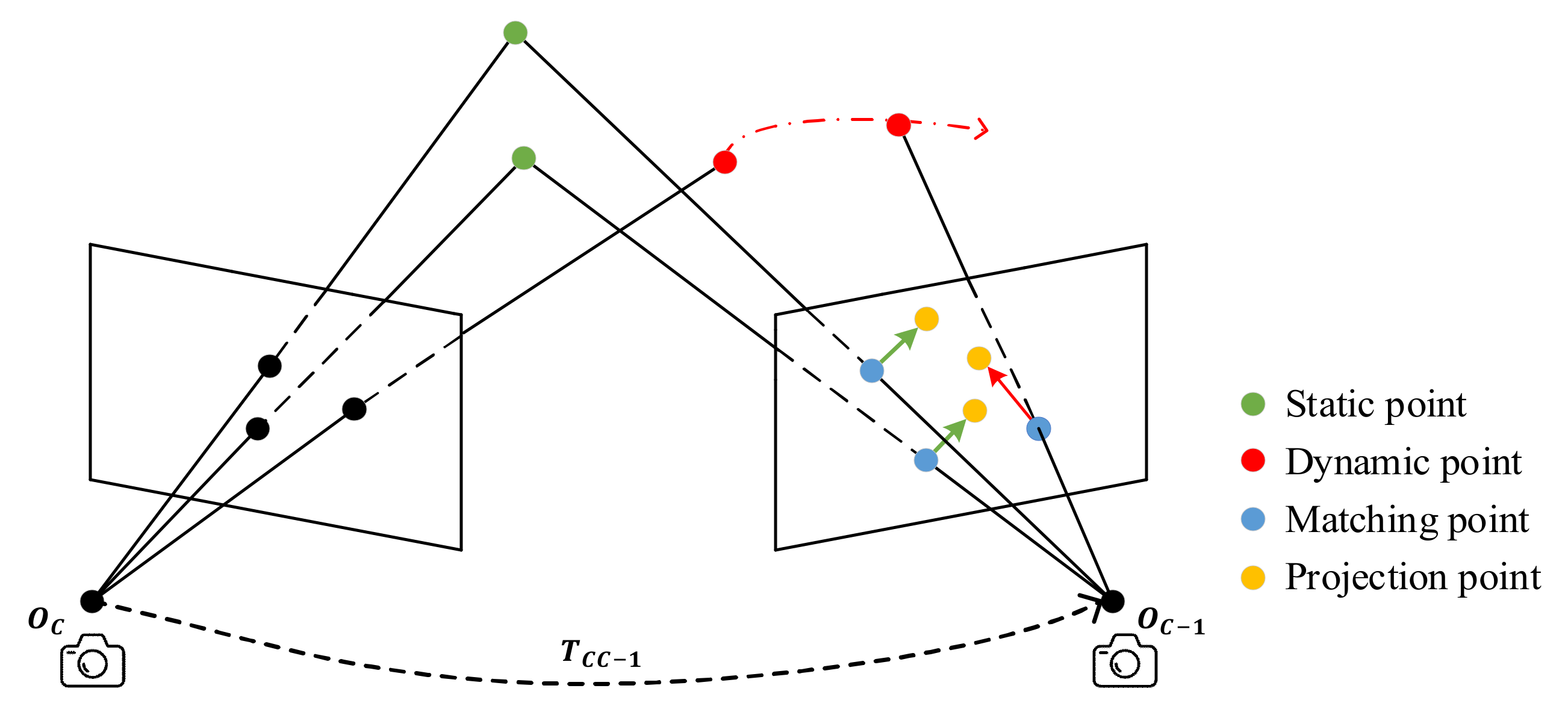
The data residual r D is the most important part of the residual model. As shown in Figure 5, the initial camera pose T cc 1 calculated by coarse tracking transforms the projection of feature points from the previous frame to the current frame (yellow points). Due to noise and initial pose errors, the static projection point and the matching point (green point) often do not coincide, but their distances and directions are usually similar (green arrows). However, the projection points corresponding to the dynamic points (red points) are significantly different from the matching points in both size and direction (red arrows) from the static points. The dynamic regions in the image can be determined based on this information, so we construct the data residual term r D :
r D = r Z + α i r I
where r Z and r I represent the pixel depth and intensity residual, respectively. α i is the weight to balance the contribution of depth residuals and intensity residuals. The depth residual r z i and intensity residual r I i of cluster c i can be calculated, respectively, as:
r z i = 1 n     Z ¯ j c i n || Z p j || T cc 1 π 1 p j 1 , Z p j 1 | z | | 2
r I i = 1 n j c i n || I p j 1 ( p j 1 ) | | 2
where p j 1 2 is the pixel coordinate of the previous frame, and current frame pixel p j is the projection point of p j 1 . Z ¯ is the average depth of c i , n is the number of pixels in c i , and | | z represents the Z coordinate values of the 3D points. Z x and I x represent the depth and intensity of pixels, respectively. Intensity is converted from the color image (0.299R + 0.587G + 0.114B), and depth is from the depth image. The function π 1 :   2 3 projects 2D point p = u , v to 3D point P = X , Y , Z according to the pinhole model as follows:
P = π 1 p , Z = u o x f , v o y f , Z
where o x , o y is the camera principal point.
In theory, if the initial pose T cc 1 is accurate, then static objects have low depth and intensity residuals, while moving objects have high residuals. Dynamic targets can be detected based on the data residual. However, in practice the process is much more complicated because data residual is not always a good metric to evaluate precise image alignment. Therefore, we borrow and improve the idea of Jaimez’s method [15] and add spatial residual.
The purpose of spatial residual r S is to encourage contiguous clusters of the same object have similar segmentation results. As shown in 
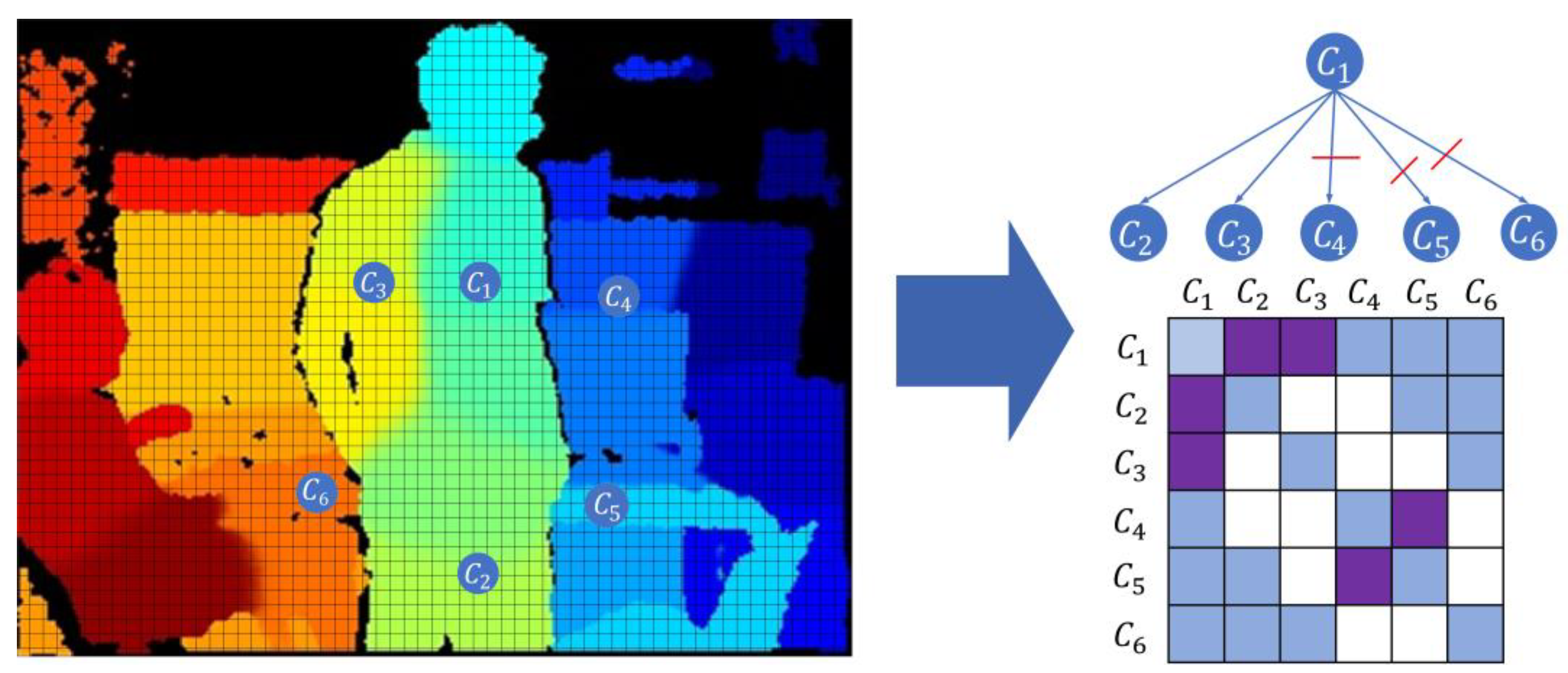
Figure 6, the person is divided into several adjacent clusters after K-means clustering, but they may have similar motion states. Therefore, we build the connectivity graph by determining the clusters’ spatial connectivity status and correlation, which assists in computing the spatial residual r S . The specific steps are as follows:
  • Statistically analyze the spatial connectivity of the clustering and compute the average depth difference Δ Z ¯ of the boundary pixels of each pair of neighboring clusters as:
    Δ Z i ¯ = 1 n k = 1 n Z C i k - C j k  
    where C i k and C j k are the neighboring clusters and n is the number of neighboring cluster boundary pixels. Z(x)∈R represent the depth of pixels.
  • Compare Δ Z i ¯ with the threshold value Δ Z t . If Δ Z i ¯ is less than Δ Z t , the two clusters are spatially correlated. Then we can build the connectivity graph as shown in Figure 6. Finally, based on the connectivity graph, the spatial residual r R i of cluster c i is calculated as:
    r R i = λ R j = 1 K G ij r D j r D i
    where K is the number of spatially connected clusters to the cluster c i . r D i and r D j are the data item residuals of clusters i and j, respectively. G ij is the clustering correlation function: it is equal to 1 when clusters i and j are spatially correlated and is 0 otherwise.
Figure 6. The process of building connectivity graph. C 1 to C 6 are the clusters after K-means clustering. The table on the right shows its connectivity graph. The blue cells indicate that two clusters have spatial connectivity, and the purple cells indicate that two clusters have spatial connectivity and spatial correlation.
Remotesensing 14 00795 g006
In addition, we believe that the objects in the scene always tend to keep the previous motion state in a shorter period, so we add the a priori residual term r P . r P contains two parts: the residual r i 1 of the previous frame and the residual r S i 1 of the corresponding region in the semantic mask of the previous frame. The priori residual r P i   of cluster c i is defined as:
r P i = λ T n j c i n r i 1 p j 1 + r S i 1 p j 1 r D i p j
where p j 1 is the pixel coordinate of previous frame, p j is the is the projection point of p j 1 in current frame, n is the number of pixels in c i . If previous frame is semantic frame and p j 1 is included in the semantic mask, r S i 1 p j 1 = 0.3 , else r S i 1 p j 1 = 0 .

3.1.3. Scene Motion Segmentation
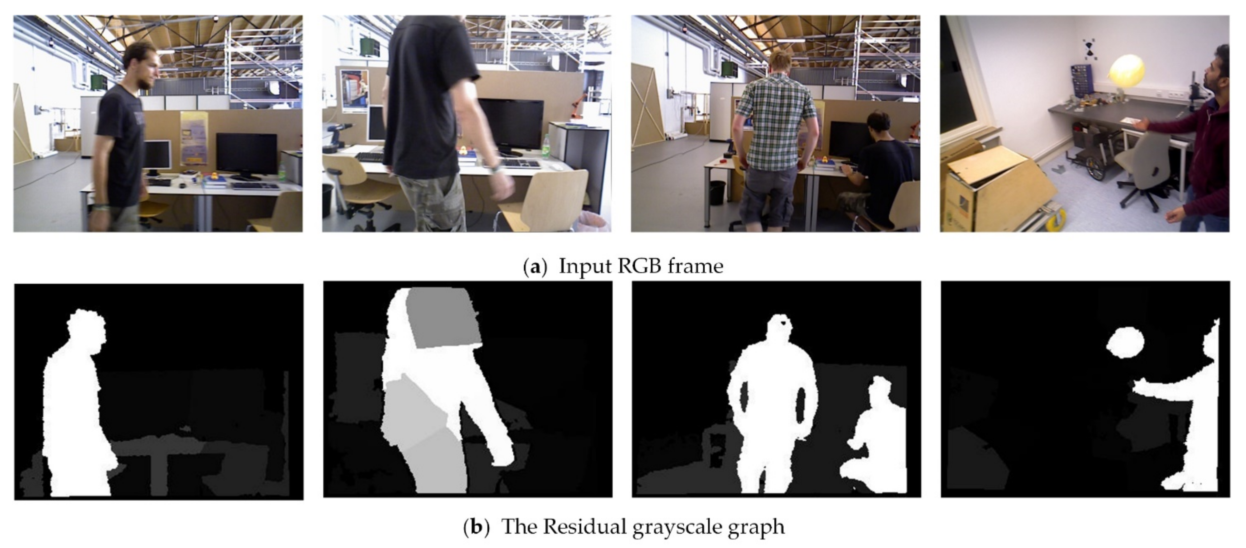
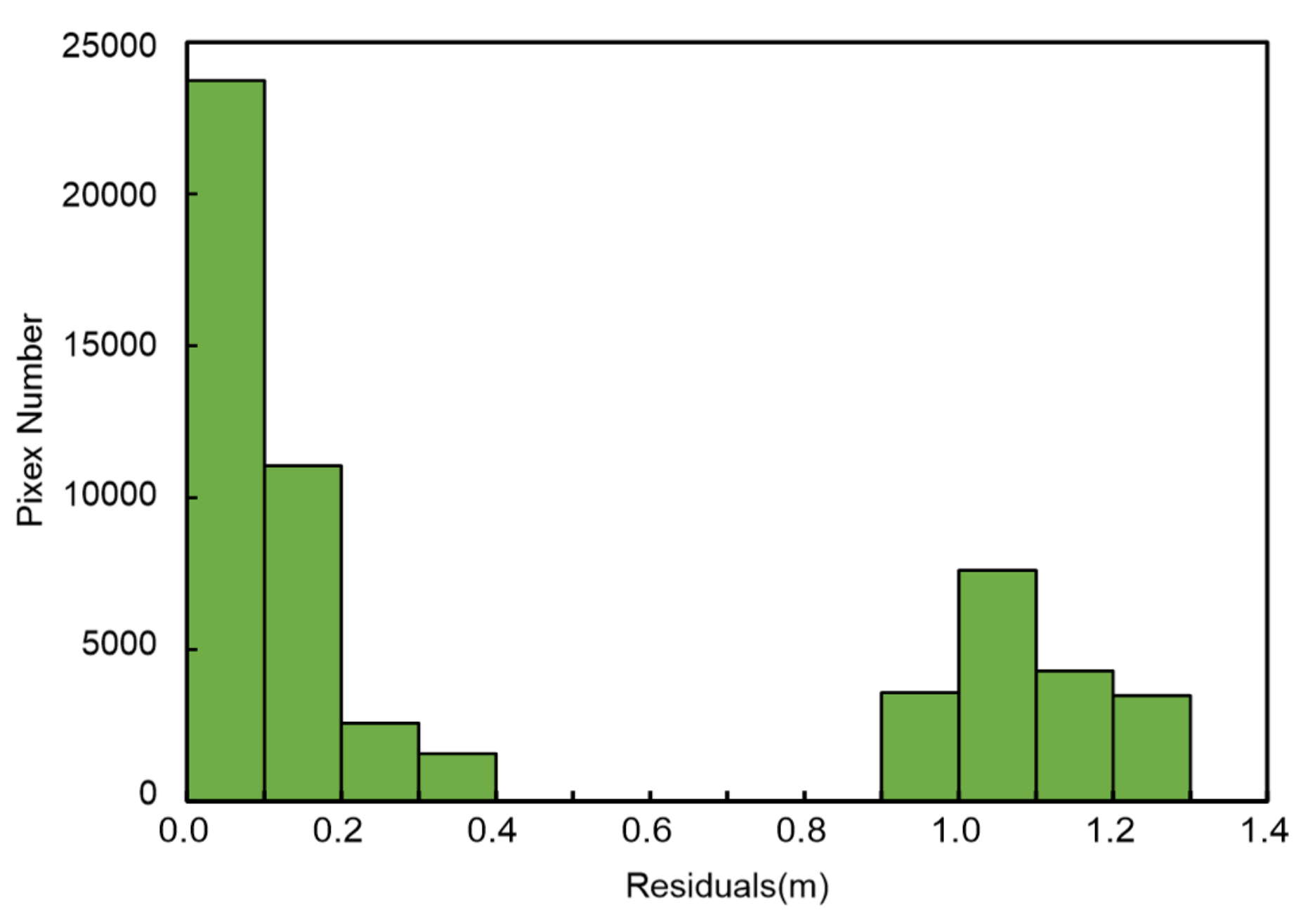
As shown in Figure 7, the residual gray graph generated by the residual model shows that the residual values of static and dynamic objects are significantly different. Because the motion of the dynamic object itself is independent of the camera, it has a high residual. The residual of static objects is usually small or close to zero. However, the residual distribution is not always the same in different scenarios, so it is difficult to divide the high and low residuals through a fixed threshold. Therefore, we design an adaptive threshold algorithm to realize scene motion segmentation.
Considering the residual distribution of each cluster and the semantic information of the instance segmentation, we define the adaptive residual threshold T as:
T = α T C + 1 α T S
where T C is a residual distribution threshold calculated based on the residual distribution of the current frame, and T S is a semantic residual threshold calculated based on the weighting of historical semantic frames. α serves to balance the current frame and historical semantic frames. A higher value implies more sensitivity to the current segmentation result. Otherwise, it indicates more consideration of historical information from semantic detection. In our experiments, we set α = 0.7. Because semantic detection is unreliable in some scenes, it is easy to treat stationary people or cars as dynamic objects, thus lowering the threshold to misclassify other static objects as dynamic.
A.
Residual Distribution Threshold T C
Figure 8 shows an example histogram of the residual distribution for a highly dynamic scene. The residual distribution consists of two distinct peaks corresponding to the residuals in the static and dynamic regions. If the trough between the two peaks can be identified as a threshold, the two types of objects can be easily separated. However, the residual distribution is often discontinuous, with spikes and jitter, making it difficult to calculate an accurate cutoff point. We extend the idea of the Otsu [40] method to segment the histogram of residual distribution for each frame, which is used to calculate the residual value T C between the dynamic objects and static objects. The specific calculation process is as follows:
  • Compute the normalized residuals histogram. Assume that the initial threshold T 0 divides the histogram into two parts, namely dynamic objects D and static objects S. Let n i be the number of pixels in cluster I, N S be the number of static object pixels, N D be the number of dynamic objects pixels, and K be the number of image clusters. Then, the normalized value p i is
p i = n i N S .
  • Calculate the pixel ratio ω s and the average residual value m S for static objects in the range [0, k]:
ω s = i S n i N S + N D
m S = i S r i p i
  • Calculate the global average residual m H :
m H = i = 1 K r i p i
  • Calculate the inter-class variance between dynamic and static objects:
σ 2 = ω s m S m H 2 + ω d m D m H 2
  • The threshold T C is the value of k that maximizes σ 2 :
T C = argmaxσ 2   k
Figure 8. Example of a residuals histogram in a highly dynamic scene.
Remotesensing 14 00795 g008
When the scene is static, the threshold T is calculated to be small, which will incorrectly classify some static objects as dynamic. We set the segmentation function to adjust the threshold T to suit different application scenarios.
0.2 ,   if   T C < 0.2 T C ,   if   T C > 0.2
B.
Semantic Residual Threshold T S
In addition, we use the semantic segmentation results to calculate the semantic residual threshold T S to improve the reliability of the adaptive threshold T. Instance segmentation cannot determine whether the target is moving or not, so we choose the five frames with the highest overlap to calculate T S . First, we traverse the semantic frame database and calculate the overlap O i between the semantic frame and the current frame by the rotation matrix R and the translation vector t:
O i = 0.7 || R i R C | | 2 + 0.3 || t i t C | | 2
Second, we select the five frames with the highest overlap among them and calculate the average residual value T S i of the semantic maskfor each frame:
T S i = 1 n s j = 1 n s r j
where n s is the number of semantic frame mask pixels. Finally, we calculate the semantic residual threshold T s based on the overlap weighting and average residual T S i of each semantic frame:
T S = i = 5 5 O i T S i j = 0 5 O i
We input T C and T S into Equation (9) to calculate the adaptive threshold T for the current frame. We then use T to classify the clusters of the current frame and determine their motion state:
Status C i = static , r i < T 2 unknown , T 2 < r i < T dynamic , r i > T

3.2. Camera Ego-Motion Estimation

Through the dynamic object detection module, we can generate the mask of dynamic objects. Because the segmentation boundaries of the mask are high-gradient areas, a large number of feature points will be detected. In practice, the segmentation of object boundaries is sometimes unreliable, as shown in Figure 9. If directly applying the mask image, many dynamic feature points will be detected at the boundaries of the mask. Therefore, we dilate the mask to fill the holes and expand object boundaries.
As shown in Figure 10, after the dilation operation, we classified the feature points into three subsets based on the region’s motion state: dynamic, static, and unknown subsets. Based on the feature point classification results, we modify the tracking threads of 3. First, for the static feature of the previous frame, their matches in the current frame are found by comparing the ORB descriptor distances. Then, to reduce the influence of dynamic objects, we remove the dynamic feature points. Finally, for the remaining two types of feature points, we use static feature points to estimate the camera ego-motion. If the number of static feature points is insufficient, we also use feature points from the unknown subset. If the tracking still fails, we use feature points in the dynamic subset to guarantee camera tracking. In addition, we further optimize the camera poses by loop closing and full BA to make the pose estimation more robust and accurate.

3.3. Semantic Segmentation Module

The dynamic object detection module can segment dynamic objects without semantic information. However, when the dynamic objects of the scene or the camera pose change drastically, the geometric information alone is not sufficient to support the dynamic object detection module to segment the dynamic scene robustly in the long term. Therefore, we design the semantic segmentation module, which can perform instance segmentation when appropriate to provide the dynamic object detection module with potential motion information of the scene.

3.3.1. Semantic Frame Selection Strategy

To detect dynamic objects using semantic information, most current semantic dynamic SLAM algorithms need to extract the semantic information of each input frame, which consumes many computational resources and is difficult to run in real-time or at high speed. In addition, some dynamic SLAMs use keyframe-based semantic detection to save time. However, their keyframe extraction strategy only continues the original platform’s strategy and has not been changed for dynamic environments. Unlike them, we design the semantic frame selection strategy according to the changes of dynamic objects in the scene and the camera motion. This strategy not only ensures that there is enough prior information of dynamic objects when the scene and objects change but also greatly reduces the computing cost of the system. Our specific semantic frame selection strategy is shown as follows:
1.
The static tracking points of the current frame are less than 10% of the total feature points.
2.
The pixel ratio of the dynamic objects in two consecutive frames is higher than 20% of the average ratio of the previous five frames, and the dynamic objects occupy at least 10% of the scene area.
3.
The average relative change in translation and rotation of the three adjacent frames is higher than 50% of the average transformation of the previous five frames. The relative changes in translation Δ t and rotation Δ R are defined as:
Δ t = || t cur t last || Δ R = arccos tr R cur R last T 1 2
where t cur and t last represent the current frame and previous frame translation vector, respectively; R cur and R last are the current frame and previous frame rotation matrix, respectively; tr · stands for the trace of a matrix.
4.
No new semantic frame were generated for 30 consecutive frames.
The purpose of design strategy 1 is to improve the segmentation accuracy through semantic segmentation when the dynamic object detection module incorrectly divides static objects into dynamic objects, resulting in too few static tracking points. The condition of strategy 2 is that when the proportion of dynamic pixels in the scene increases significantly, it indicates that new dynamic objects enter the scene or some objects are changing their mobility. At this time, semantic segmentation provides motion a priori information so that the dynamic object detection module can better segment and track dynamic objects. Strategy 3 is established because when the camera rotates or translates rapidly, it may not be able to segment the scene accurately only by geometric detection, and semantic detection is needed to provide more information. Strategy 4 updates the semantic input information in the dynamic object detection module and improves the system’s robustness for long-term operation. In addition, to avoid wasting system computing resources, we do not select semantic frames within five frames after the previous semantic frame. In other cases, as long as any strategy is satisfied, the input frame is recognized as a semantic frame and performs instance segmentation.

3.3.2. Segmentation of Potentially Moving Objects

To ensure the speed and accuracy of segmentation, we choose the lightweight one-stage segmentation network YOLACT++ (You Only Look At CoefficienTs) [41,42] to segment RGB images pixel-wise and generate masks of potential moving objects. YOLACT++ is pre-trained on the MS COCO [43] dataset and can classify 80 classes of targets. Moreover, YOLACT++ has near real-time dynamic object segmentation capability and can achieve an accuracy of 34.1 mAP at 33.5 fps, which is very close to the current SOTA model.
For the objects detected by YOLACT++, we process only the potential objects among them, such as people, cars, and animals. The masks of these objects are input to the dynamic object detection module as a priori information to assist the system in the segmentation of dynamic objects (Figure 11).

4. Experimental Results and Analysis

To evaluate the effectiveness of DGS-SLAM, we conducted a series of experiments on two public dynamic scene datasets. First, we quantitatively evaluated and analyzed the semantic selection strategy of DGS-SLAM. Then, the experimental results of the system in different configurations were analyzed and compared with the original ORB-SLAM3 (RGB-D mode only without IMU) to quantify the improvement of DGS-SLAM in dynamic scenes. Finally, we marked a comparative analysis with the most advanced dynamic RGB-D SLAM methods (including semantic-based and geometry-based methods).
All experiments were performed on an AMD 5900HX laptop with 16 GB RAM and an Nvidia GPU GTX3070. For the semantic segmentation module, we used the Resnet50-FPN model pre-trained on the COCO dataset in the encoder part. For the dynamic object detection module, we down-sampled the input RGB-D image to 320*240, and the other parameters in the experiments are shown in Table 1. These parameters were determined through several experiments and experience and had some impact on the performance.
The error metrics for evaluation were the commonly-used root-mean-square-error (RMSE) of the absolute trajectory error (ATE) [44] in m, and RMSE of the relative pose Error (RPE), which comprises the translational drift in m/s and rotational drift in °/s. The ATE measures the global consistency of the trajectory, and RPE measures the odometer drift per second. We evaluated the tracking accuracy and demonstrated the performance by comparing with state-of-the-art VSLAM methods using, when possible, the results from the original papers.

4.1. TUM RGB-D Dataset

The TUM RGB-D dataset [44] consists of RGB and depth images (640x480) collected by a Kinect RGB-D camera at 30 Hz frame rate and camera ground truth trajectories obtained from a high precision motion capture system. It includes 39 indoor scene sequences, of which we selected dynamic sequences to evaluate our system. We divided these dynamic sequences into two categories: low and high dynamic sequences. The low dynamic sequences included three fr3/sitting (fr3/s for short) sequences: fr3/s_xyz, fr3/s_half, and fr3/s_xyz. In these sequences, two people sit at a table with slight body movements. The highly dynamic sequences contain four fr3/walking (fr3/w for short) sequences: fr3/w_half, fr3/w_rpy, fr3/w_static, and fr3/w_xyz. In the highly dynamic sequences, two people walk quickly around the table in the office. These sequences are very challenging for SLAM systems because dynamic objects occupy a large portion of the camera view.
First, we quantitatively evaluated the semantic frame selection strategy of DGS-SLAM. We integrated the designed semantic frame-based and the currently popular keyframe-based strategy into DGS-SLAM separately and conducted comparative experiments. The number of semantic segmentations and the ATE values for each of the two strategies are shown in Table 2. It can be seen that the DGS-SLAM based on the semantic frame strategy performed fewer semantic segmentations while obtaining lower ATE. Because the keyframe selection strategy selects frames with good quality and low overlap to represent local frames, it is intended for relocalization, loop closing, and full BA. It is not suitable as a judgment basis for performing semantic detection. In contrast, our semantic frame selection strategy was designed based on the segmentation results of dynamic object detection and the motion changes of the scene. It can provide semantic information when the segmentation results are unstable, the dynamic objects of the scene change, and the camera moves violently to maintain the system’s stable operation.
Second, we visualized the performance of DGS-SLAM in two highly dynamic sequences. As shown in Figure 12, we used an open-source measurement tool evo (github.com/MichaelGrupp/evo (accessed on 26 December 2021).) to plot the ATE distribution curves for the two highly dynamic sequences. The blue line represents the ATE of the original ORB-SLAM3, and the green line represents the ATE after eliminating the effect of dynamic objects by our method. When dynamic objects appeared in the scene, the ATE of ORB-SLAM3 increased dramatically. However, our method dramatically reduced the ATE value of the system at the same moment by removing the dynamic objects in the scene and tracking only the reliable static points.
Then, we evaluated the accuracy of the system in different configurations and compared it with the original ORB-SLAM3 (RGB-D mode only without IMU). In this case, DGS-SLAM (S) removed dynamic objects using only the YOLACT++ network for each image frame. DGS-SLAM (G) performed motion segmentation of the scene using only the geometric part of the dynamic object detection module, where the semantic input information in the residual model and adaptive thresholding was zero. DGS-SLAM combined semantic and geometric information and used all the functions of our system.
As shown in Table 3, for low dynamic sequences, our algorithm had similar accuracy as ORB-SLAM3. Because the two people in the scene had only slight movements, ORB-SLAM3 had strong robustness using a uniformized feature extraction strategy and the RANSAC algorithm to filter some outlier anomalies effectively. In addition, low dynamic motion was usually not continuous in the sequence, and the moving objects were always stationary in some frames. Therefore, the overall improvement of our method was limited. For highly dynamic sequences, the dynamic objects in the scene occupied a large proportion of the region, which could not be filtered by the original optimization strategy of the ORB-SLAM3 algorithm. In contrast, our method could remove the influence of dynamic objects in the scene on camera ego-motion estimation. Therefore, DGS-SLAM(G), DGS-SLAM(S), and DGS-SLAM all achieved significant improvements in accuracy, and DGS-SLAM combining semantic and geometric information achieved the highest accuracy. In addition, to illustrate the system improvement more visually, we plotted the ATE distribution of DGS-SLAM with different configurations versus ORB-SLAM3 for low and high dynamic sequences using the evo tool (see Figure 13).
Finally, we compared the experimental results of DGS-SLAM with the current state-of-the-art dynamic VSLAM algorithms, including the geometry-based algorithms, VO-SF [18], StaticFusion [15], and the DSLAM [14]; and the semantic-based algorithms, DS-SLAM [29], DynaSLAM [30], KMOP-VSLAM [25], and RDMO-SLAM [24]. Table 4, Table 5 and Table 6 summarize the comparison results of ATE and RPE, respectively. In low dynamic scenes, our method almost achieved the highest localization accuracy for two main reasons. One is that our system was based on ORB-SLAM3, one of the most stable VSLAM systems at present, with perfect back-end optimization and loop closing. Second, our system was different from other semantic-based methods that rely excessively on semantic segmentation network results. We only input the semantic segmentation results into the residual model and adaptive thresholding in the dynamic object detection module to assist its segmentation for dynamic objects. As shown in Figure 14, the person on the left in the scene remained stationary, and the person on the right had an upper limb swinging action. Instead of removing the whole semantic network output mask, our system removed only the motion part through the dynamic object detection module. This increased the number of reliable feature points and improved the localization accuracy.
In highly dynamic scenes, our approach outperformed most algorithms and achieved similar results to DynaSLAM. However, unlike their strategy for semantic detection, we only performed instance segmentation on semantic frames, and the other frames were dynamically segmented only by the efficient dynamic object detection module. In addition, in the dynamic object detection module, we down-sampled the input RGB and depth images to improve the computational speed. As a result, we achieved similar performance with less time and semantic information. Later we analyzed our runtime. The trajectories of DGS-SLAM and ORB-SLAM3, DynaSLAM, and RDS-SLAM in highly dynamic scenes are shown in Figure 15, which also demonstrate that our algorithm had reliable accuracy of bit pose estimation in dynamic scenes.

4.2. Bonn RGB-D Dynamic Dataset

Our second dataset used the Bonn RGB-D dynamic dataset [13], provided by the University of Bonn. This dataset acquired RGB-D images by ASUS Xtion Pro LIVE and camera ground truth trajectories with an Optitrack Prime 13 motion capture system. The Bonn dataset includes 24 highly dynamic scenes where people perform different tasks, such as carrying boxes and playing with balloons. Moreover, in some scenes, dynamic scenes occupy most of the scene, which extremely tests the robustness of the SLAM algorithm.
First, we evaluated the results of dynamic object detection. Comparing DGS-SLAM with DynaSLAM (which has the highest segmentation accuracy in dynamic SLAM), the results are shown in Figure 16. Figure 16a shows the experimenter in the scene playing a balloon with a fast-moving speed. The instance segmentation network did not detect the moving balloon and even incorrectly determined the stationary wooden box as a moving object. DynaSLAM inherits the segmentation results from the semantic detection network, and its multi-view geometry method did not detect the balloon either. However, our method only used the a priori information input from the semantic segmentation module to assist the dynamic object detection module in segmenting moving objects, which was less affected by its segmentation results. The results also showed that our method successfully detected the balloon and was not affected by the results of semantic detection network errors. Figure 16b shows the three experimenters moving rapidly in the scene, and one of them was holding a laptop computer. The moving persons were successfully detected in the mask output by the instance segmentation network, but the laptop was not detected. The laptop was not an a priori moving object but was carried by people to change its position. DynaSLAM and DGS-SLAM could not only detect the moving experimenter in the scene but also successfully detected the carried laptop by the geometric algorithm.
Then, we compared our tracing performance with counterpart state-of-the-art VSLAMs, namely ORB-SLAM3, StaticFusion, ReFusion [13], and DynaSLAM methods in the Bonn RGB-D dynamic dataset, as shown in Table 7. In low dynamic sequences, where dynamic objects occupied a small proportion of the scene, our method had limited improvement over ORB-SLAM3 and other methods. In highly dynamic scene sequences, DGS-SLAM achieved similar or better localization accuracy than DynaSLAM and substantially outperformed the other methods. However, in some sequences, DynaSLAM did not achieve robust tracking in the long term. For example, DynaSLAM lost tracking in the moving_obstructing_box and moving_obstructing_box2 sequences. In the moving_obstructing_box sequence shown in Figure 17, the moving person and the box occupied the whole scene, and the box surface was flat and lacked texture features. After DGS-SLAM and DynaSLAM deleted the dynamic area, the static feature points were not sufficient to continue tracking the camera. However, we improved the tracking strategy of dynamic SLAM so that DGS-SLAM tracked dynamic and unknown feature points to ensure continuous camera tracking after lost tracking. DynaSLAM did not take any measures to cause tracking failure. In conclusion, our method had stronger robustness than other methods while maintaining high tracking accuracy in dynamic scenes.

4.3. Running Time Analysis

To evaluate the DGS-SLAM efficiency, we counted the average running time of the different modules. Table 8 shows the total frames, semantic frames, and average running times of DGS-SLAM for some sequences on two dynamic datasets. The average running time of DGS-SLAM processing each frame fluctuated between 34 and 38 ms. Because our segmentation strategy was only instance segmentation of semantic frames, each segmentation took a lot of time. Therefore, the proportion of semantic frames greatly influenced the overall running time. For example, in highly dynamic sequences such as fr3/w_half and fr3/w_rpy, dynamic objects moved frequently and required high robustness of the SLAM system. To ensure the tracking accuracy of the camera, the semantic frame selection strategy we designed notably increased the number of semantic frames, which also increased the overall running time of the system accordingly. However, our other modules had high efficiency, and the proposed system could maintain a running frame rate above 25 Hz.
Table 9 compares the execution time of DGS-SLAM with the original ORB-SLAM3, DS-SLAM, and DynaSLAM under the same computing platform. It can be seen that DGS-SLAM had an advantage in both semantic segmentation and dynamic object detection modules in terms of computing time. In the dynamic object detection module, DGS-SLAM only determined the cluster motility instead of segmenting pixel-wise, which significantly simplified the complexity of segmentation. To further accelerate detection, we also downsampled input RGB-D images to reduce the amount of computed data. In the semantic detection module, we used the lightweight instance segmentation network YOLACT++, which could segment at 30 FPS with RTX 3070. Moreover, unlike DS-SLAM and DynaSLAM, which perform instance segmentation for all frames, we only extracted semantic information of semantic frames to assist the lightweight dynamic object detection module in segmenting each scene frame, which greatly sped up the operation of the system. Overall, the operating frame rate of the system could reach more than 25 Hz, which essentially achieved the requirement of real-time operation. Moreover, the real-time performance of DGS-SLAM could be further improved with the improvement of experimental conditions.

5. Discussion

In this paper, we propose an RGB-D SLAM system combined with geometric and semantic information, which can run fast and robustly in dynamic environments. Traditional geometry-based SLAM methods are less accurate than semantic-based SLAM methods in dynamic environments under normal conditions. However, semantic-based SLAM methods have difficulty meeting the real-time requirements of SLAM systems in terms of runtime. In this case, we innovatively design a semantic frame selection strategy and propose a dynamic object detection method based on a residual model. The system can reach a good balance between pose estimation accuracy and time efficiency. To evaluate the experiment’s reliability, we compare the performance of various SLAM algorithms with our method on the TUM and Bonn datasets. The experimental results demonstrate the strong localization accuracy and efficient system runtime of the algorithm in dynamic environments.
First, we combine data residuals, spatial residuals, and a priori residuals of geometric and semantic information to design a multinomial residual model calculation method. An adaptive residual threshold algorithm is proposed using previous residual results. The algorithm combines the weighted residual threshold of the historical semantic frame and the residual distribution threshold of the current frame, which enhances the detection ability of dynamic targets. Second, the general keyframe selection strategy in the SLAM systems is not suitable for semantic detection, while we design a semantic frame selection strategy with static tracking points, dynamic pixel occupation probability, and camera pose change threshold, taking into account the changes of dynamic objects and camera motion in the scene. The proposed method greatly reduces the computational cost and increases the robustness of the system.
In terms of robustness of localization and camera ego-motion estimation, the system’s overall performance was evaluated and validated in this paper on two dynamic datasets and compared with the most advanced algorithms based on geometry and semantics. The results for ATE and RPE are presented in Table 4, Table 5 and Table 6. DGS-SLAM obtains the most competitive experimental results for high and low dynamic sequences. In contrast to ORBSLAM3, it is based on the assumption of a static world, resulting in lower accuracy among dynamic scenarios. We propose an integrated residual model and adaptive thresholding for dynamic object detection, which substantially improves the localization accuracy and increases the robustness of the ORB-SLAM3 system in highly dynamic scenes. Compared with the most popular system DynaSLAM, which directly removes potential motion targets as dynamic regions, the proposed algorithm inputs potential motion information into the dynamic object detection module to further determine their true motion. This strategy can improve the positioning accuracy of the system. In addition, our algorithm modifies the tracking strategy of the camera to improve the system’s ability to continuously track in highly dynamic scenes compared to DynaSLAM.
In terms of computational efficiency, this paper compared the average running times of DGS-SLAM and other SLAM systems on two datasets. From Table 9, it is clear that DGS-SLAM has a great advantage in terms of computing time compared to the DS-SLAM and DynaSLAM semantic-based SLAM algorithms. In the dynamic object detection module, we only determine the motion of the clusters and do not perform pixel-wise segmentation. In the semantic segmentation module, we do not semantically segment all frames but only extract the semantic information of the semantic frames, which greatly accelerates the operation speed of the system.

6. Conclusions

In this paper, we propose a robust RGB-D SLAM system for dynamic environments. To reduce the impact of dynamic objects on camera ego-motion estimation, we design a semantic segmentation module based on semantic frames and a dynamic object detection module based on residual models. Among them, the semantic segmentation module combines the motion of the scene and the dynamic object to judge the input frames. If the semantic frame selection strategy is satisfied, instance segmentation is performed to generate masks of potential dynamic objects and input to the dynamic object detection module as a priori motion information. The dynamic object detection module first performs spatial clustering on the current frame. Then it combines geometric and prior information to build a residual model. Finally, we use the a priori motion information of the historical semantic frames and the geometric residual information of the current frame to calculate the adaptive threshold to segment the scene. In addition, we improve the tracking algorithm of ORB-SLAM3 in combination with the detection results to be able to work consistently and robustly in dynamic environments.
We performed quantitative evaluations on the challenging TUM RGB-D dataset as well as the Bonn RGB-D dynamic dataset and compared the results with other state-of-the-art dynamic VSLAM methods. The experimental results show that our method achieves state-of-the-art localization accuracy and robustness in dynamic environments while maintaining near real-time operation speed.
In future work, we plan to extend the DGS-SLAM in two directions. First, we will introduce learning-based deep clustering methods, such as PCIA [45], to further improve segmentation results. Second, we will explore the tracking and prediction of dynamic targets, which is the basis for multi-robot collaboration, virtual reality, and autonomous driving work.

Author Contributions

X.H.; Data curation, H.X.; Funding acquisition, L.Y.; Investigation, X.H., Y. C. and P.W.; Methodology, Li Yan, Xiao Hu and L.Z.; Project administration, X.H.; Resources, Y.C. and H.X.; Software, X.H.; Supervision, L.Z. and P.W.; Visualization, X.H.; Writing—review & editing, L.Z. and X.H. All authors have read and agreed to the published version of the manuscript.

Funding

National Key Research and Development Project of China: 2020YFD1100200; The Science and Technology Major Project of Hubei Province under Grant: 2021AAA010.

Conflicts of Interest

The authors declare no conflict of interest.

References

  1. Cadena, C.; Carlone, L.; Carrillo, H.; Latif, Y.; Scaramuzza, D.; Neira, J.; Reid, I.; Leonard, J.J. Past, Present, and Future of Simultaneous Localization and Mapping: Toward the Robust-Perception Age. IEEE Trans. Robot. 2016, 32, 1309–1332. [Google Scholar] [CrossRef] [Green Version]
  2. Zhao, Y.; Yan, L.; Chen, Y.; Dai, J.; Liu, Y. Robust and Efficient Trajectory Replanning Based on Guiding Path for Quadrotor Fast Autonomous Flight. Remote. Sens. 2021, 13, 972. [Google Scholar] [CrossRef]
  3. Zhao, L.; Yan, L.; Hu, X.; Yuan, J.; Liu, Z. Efficient and High Path Quality Autonomous Exploration and Trajectory Planning of UAV in an Unknown Environment. ISPRS Int. J. Geo-Inf. 2021, 10, 631. [Google Scholar] [CrossRef]
  4. Dai, J.; Yan, L.; Liu, H.; Chen, C.; Huo, L. An Offline Coarse-To-Fine Precision Optimization Algorithm for 3D Laser SLAM Point Cloud. Remote. Sens. 2019, 11, 2352. [Google Scholar] [CrossRef] [Green Version]
  5. Chen, Y.; Yan, L.; Xu, B.; Liu, Y. Multi-Stage Matching Approach for Mobile Platform Visual Imagery. IEEE Access 2019, 7, 160523–160535. [Google Scholar] [CrossRef]
  6. Engel, J.; Schöps, T.; Cremers, D. LSD-SLAM: Large-Scale Direct Monocular SLAM. In Proceedings of the Computer Vision – ECCV 2014, Zurich, Switzerland, 6–12 September 2014; Springer International Publishing: Cham, Switzerland, 2014; pp. 834–849. [Google Scholar]
  7. Engel, J.; Koltun, V.; Cremers, D. Direct Sparse Odometry. IEEE Trans. Pattern Anal. Mach. Intell. 2018, 40, 611–625. [Google Scholar] [CrossRef]
  8. Mur-Artal, R.; Tardós, J.D. ORB-SLAM2: An Open-Source SLAM System for Monocular, Stereo, and RGB-D Cameras. IEEE Trans. Robot. 2017, 33, 1255–1262. [Google Scholar] [CrossRef] [Green Version]
  9. Fischler, M.A.; Bolles, R.C. Random Sample Consensus: A Paradigm for Model Fitting with Applications to Image Analysis and Automated Cartography. In Readings in Computer Vision; Elsevier: Amsterdam, The Netherlands, 1987; pp. 726–740. [Google Scholar]
  10. Fu, D.; Xia, H.; Qiao, Y. Monocular Visual-Inertial Navigation for Dynamic Environment. Remote. Sens. 2021, 13, 1610. [Google Scholar] [CrossRef]
  11. Wang, R.; Wan, W.; Wang, Y.; Di, K. A New RGB-D SLAM Method with Moving Object Detection for Dynamic Indoor Scenes. Remote Sensing 2019, 11, 1143. [Google Scholar] [CrossRef] [Green Version]
  12. Sun, Y.; Liu, M.; Meng, M.Q.-H. Motion Removal for Reliable RGB-D SLAM in Dynamic Environments. Robot. Auton. Syst. 2018, 108, 115–128. [Google Scholar] [CrossRef]
  13. Palazzolo, E.; Behley, J.; Lottes, P.; Giguère, P.; Stachniss, C. ReFusion: 3D Reconstruction in Dynamic Environments for RGB-D Cameras Exploiting Residuals. In Proceedings of the 2019 IEEE/RSJ International Conference on Intelligent Robots and Systems (IROS), Macau, China, 3–8 November 2019; pp. 7855–7862. [Google Scholar]
  14. Dai, W.; Zhang, Y.; Li, P.; Fang, Z.; Scherer, S. RGB-D SLAM in Dynamic Environments Using Point Correlations. IEEE Trans. Pattern Anal. Mach. Intell. 2020, 44, 373–389. [Google Scholar] [CrossRef]
  15. Scona, R.; Jaimez, M.; Petillot, Y.R.; Fallon, M.; Cremers, D. StaticFusion: Background Reconstruction for Dense RGB-D SLAM in Dynamic Environments. In Proceedings of the 2018 IEEE International Conference on Robotics and Automation (ICRA), Brisbane, Australia, 21–25 May 2018; pp. 3849–3856. [Google Scholar]
  16. Li, S.; Lee, D. RGB-D SLAM in Dynamic Environments Using Static Point Weighting. IEEE Robot. Autom. Lett. 2017, 2, 2263–2270. [Google Scholar] [CrossRef]
  17. Kim, D.-H.; Kim, J.-H. Effective Background Model-Based RGB-D Dense Visual Odometry in a Dynamic Environment. IEEE Trans. Robot. 2016, 32, 1565–1573. [Google Scholar] [CrossRef]
  18. Jaimez, M.; Kerl, C.; Gonzalez-Jimenez, J.; Cremers, D. Fast Odometry and Scene Flow from RGB-D Cameras Based on Geometric Clustering. In Proceedings of the 2017 IEEE International Conference on Robotics and Automation (ICRA), Singapore, 29 May–3 June 2017; pp. 3992–3999. [Google Scholar]
  19. Cheng, J.; Sun, Y.; Meng, M.Q.-H. Improving Monocular Visual SLAM in Dynamic Environments: An Optical-Flow-Based Approach. Adv. Robot. 2019, 33, 576–589. [Google Scholar] [CrossRef]
  20. Wang, Z.; Zhang, Q.; Li, J.; Zhang, S.; Liu, J. A Computationally Efficient Semantic SLAM Solution for Dynamic Scenes. Remote. Sens. 2019, 11, 1363. [Google Scholar] [CrossRef] [Green Version]
  21. Yang, D.; Bi, S.; Wang, W.; Yuan, C.; Wang, W.; Qi, X.; Cai, Y. DRE-SLAM: Dynamic RGB-D Encoder SLAM for a Differential-Drive Robot. Remote. Sens. 2019, 11, 380. [Google Scholar] [CrossRef] [Green Version]
  22. Yuan, Z.; Xu, K.; Zhou, X.; Deng, B.; Ma, Y. SVG-Loop: Semantic–Visual–Geometric Information-Based Loop Closure Detection. Remote. Sens. 2021, 13, 3520. [Google Scholar] [CrossRef]
  23. Liu, Y.; Miura, J. RDS-SLAM: Real-Time Dynamic SLAM Using Semantic Segmentation Methods. IEEE Access 2021, 9, 23772–23785. [Google Scholar] [CrossRef]
  24. Liu, Y.; Miura, J. RDMO-SLAM: Real-Time Visual SLAM for Dynamic Environments Using Semantic Label Prediction With Optical Flow. IEEE Access 2021, 9, 106981–106997. [Google Scholar] [CrossRef]
  25. Liu, Y.; Miura, J. KMOP-VSLAM: Dynamic Visual SLAM for RGB-D Cameras Using K-means and OpenPose. In Proceedings of the 2021 IEEE/SICE International Symposium on System Integration (SII), Fukushima, Japan, 11–14 January 2021; pp. 415–420. [Google Scholar]
  26. Cheng, J.; Wang, Z.; Zhou, H.; Li, L.; Yao, J. DM-SLAM: A Feature-Based SLAM System for Rigid Dynamic Scenes. ISPRS Int. J. Geo-Inf. 2020, 9, 202. [Google Scholar] [CrossRef] [Green Version]
  27. Li, A.; Wang, J.; Xu, M.; Chen, Z. DP-SLAM: A Visual SLAM with Moving Probability towards Dynamic Environments. Inf. Sci. 2021, 556, 128–142. [Google Scholar] [CrossRef]
  28. Zhong, F.; Wang, S.; Zhang, Z.; Chen, C.; Wang, Y. Detect-SLAM: Making Object Detection and SLAM Mutually Beneficial. In Proceedings of the 2018 IEEE Winter Conference on Applications of Computer Vision (WACV), Lake Tahoe, NV, USA, 12–15 March 2018; pp. 1001–1010. [Google Scholar]
  29. Yu, C.; Liu, Z.; Liu, X.-J.; Xie, F.; Yang, Y.; Wei, Q.; Fei, Q. DS-SLAM: A Semantic Visual SLAM towards Dynamic Environments. In Proceedings of the 2018 IEEE/RSJ International Conference on Intelligent Robots and Systems (IROS), Madrid, Spain, 1–5 October 2018; pp. 1168–1174. [Google Scholar]
  30. Bescos, B.; Fácil, J.M.; Civera, J.; Neira, J. DynaSLAM: Tracking, Mapping, and Inpainting in Dynamic Scenes. IEEE Robot. Autom. Lett. 2018, 3, 4076–4083. [Google Scholar] [CrossRef] [Green Version]
  31. Zhang, J.; Henein, M.; Mahony, R.; Ila, V. VDO-SLAM: A Visual Dynamic Object-Aware SLAM System. arXiv 2020, 11052. [preprint]. [Google Scholar]
  32. Davison, A.J.; Reid, I.D.; Molton, N.D.; Stasse, O. MonoSLAM: Real-Time Single Camera SLAM. IEEE Trans. Pattern Anal. Mach. Intell. 2007, 29, 1052–1067. [Google Scholar] [CrossRef] [Green Version]
  33. Yan, L.; Zhao, L. An Approach on Advanced Unscented Kalman Filter from Mobile Robot-slam. Int. Arch. Photogramm. Remote. Sens. Spat. Inf. Sci. 2020, 43, 381–389. [Google Scholar] [CrossRef]
  34. Klein, G.; Murray, D. Parallel Tracking and Mapping for Small AR Workspaces. In Proceedings of the 2007 6th IEEE and ACM International Symposium on Mixed and Augmented Reality, Nara, Japan, 13–16 November 2007; pp. 225–234. [Google Scholar]
  35. Campos, C.; Elvira, R.; Rodríguez, J.J.G.; Montiel, J.M.M.; Tardós, D.J. ORB-SLAM3: An Accurate Open-Source Library for Visual, Visual–Inertial, and Multimap SLAM. IEEE Trans. Robot. 2021, 37, 1874–1890. [Google Scholar] [CrossRef]
  36. Elvira, R.; Tardós, J.D.; Montiel, J.M.M. ORBSLAM-Atlas: A Robust and Accurate Multi-Map System. In Proceedings of the 2019 IEEE/RSJ International Conference on Intelligent Robots and Systems (IROS), Macau, China, 3–8 November 2019; pp. 6253–6259. [Google Scholar]
  37. Badrinarayanan, V.; Kendall, A.; Cipolla, R. SegNet: A Deep Convolutional Encoder-Decoder Architecture for Image Segmentation. IEEE Trans. Pattern Anal. Mach. Intell. 2017, 39, 2481–2495. [Google Scholar] [CrossRef]
  38. He, K.; Gkioxari, G.; Dollár, P.; Girshick, R. Mask R-CNN. In Proceedings of the 2017 IEEE International Conference on Computer Vision (ICCV), Venice, Italy, 22–29 October 2017; pp. 2980–2988. [Google Scholar]
  39. Liu, W.; Anguelov, D.; Erhan, D.; Szegedy, C.; Reed, S.; Fu, C.-Y.; Berg, A.C. Single Shot MultiBox Detector. In Proceedings of the Computer Vision – ECCV 2016, Amsterdam, The Netherlands, 11–14 October 2016; Leibe, B., Matas, J., Sebe, N., Welling, M., Eds.; Springer International Publishing: Cham, Switzerland, 2016; pp. 21–37. [Google Scholar]
  40. Otsu, N. A Threshold Selection Method from Gray-Level Histograms. IEEE Trans. Syst. Man Cybern. 1979, 9, 62–66. [Google Scholar] [CrossRef] [Green Version]
  41. Bolya, D.; Zhou, C.; Xiao, F.; Lee, Y.J. YOLACT: Real-Time Instance Segmentation. In Proceedings of the 2019 IEEE/CVF International Conference on Computer Vision (ICCV), Seoul, Korea, 27 October–2 November 2019; pp. 9156–9165. [Google Scholar]
  42. Bolya, D.; Zhou, C.; Xiao, F.; Lee, Y.J. YOLACT++: Better Real-Time Instance Segmentation. IEEE Trans. Pattern Anal. Mach. Intell. 2020, 1, 1. [Google Scholar] [CrossRef]
  43. Lin, T.-Y.; Maire, M.; Belongie, S.; Hays, J.; Perona, P.; Ramanan, D.; Dollár, P.; Zitnick, Z.L. Microsoft COCO: Common Objects in Context. In Proceedings of the Computer Vision – ECCV 2014, Zurich, Switzerland, 6–12 September 2014; Springer International Publishing: Cham, Switzerland; pp. 740–755. [Google Scholar]
  44. Sturm, J.; Engelhard, N.; Endres, F.; Burgard, W.; Cremers, D. A Benchmark for the Evaluation of RGB-D SLAM Systems. In Proceedings of the 2012 IEEE/RSJ International Conference on Intelligent Robots and Systems, Vilamoura-Algarve, Portugal, 7–12 October 2012; pp. 573–580. [Google Scholar]
  45. Huang, J.; Gong, S.; Zhu, X. Deep Semantic Clustering by Partition Confidence Maximisation. In Proceedings of the 2020 IEEE/CVF Conference on Computer Vision and Pattern Recognition (CVPR), Seattle, WA, USA, 13–19 June 2020; pp. 8846–8855. [Google Scholar]
Figure 2. Flowchart of the dynamic object module. The red arrows represent the input of the semantic segmentation module, and the black arrows represent the execution procedures of the dynamic object detection module.
Remotesensing 14 00795 g002
Figure 3. The input and output of K-means. (a) The input depth image. (b) The output result of K-means clustering.
Remotesensing 14 00795 g003
Figure 4. Comparison of the two ORB matching strategies. (a) Camera pose tracking by original ORB matching. (b) Camera pose tracking by the static feature points of the previous frame. The red box indicates the presence of dynamic objects in the region. Coarse tracking uses only static feature points from the previous frame, reducing the effect of dynamic objects on the matching result.
Remotesensing 14 00795 g004
Figure 5. The principle of data residual. We can evaluate the dynamic of feature points using camera ego-motion.
Remotesensing 14 00795 g005
Figure 7. Example results of the residual model. (a) The original input RGB frame. (b) The residual grayscale graph. To visualize the residual results, we make the gray value of the maximum residual 256. The rest of the clusters calculate the corresponding gray value according to the ratio of their residuals to the maximum residual and generate the residual gray map.
Remotesensing 14 00795 g007
Figure 9. Example of mask dilation. (a) The original dynamic object mask. (b) The mask after dilation. (c) The dynamic feature points before mask dilation. (d) The dynamic feature points after mask dilation. Outliers on the boundaries of dynamic objects are removed. Features in red are dynamic features, and those in green are static features.
Remotesensing 14 00795 g009
Figure 10. Classification results of feature points. The features in blue belong to unknown subset. Green features belong to static subset, and red features belong to dynamic subset.
Remotesensing 14 00795 g010
Figure 11. The input and output of YOLACT++. (a) The input RGB image. (b) The output result of YOLACT++. (c) Mask of potential moving objects.
Remotesensing 14 00795 g011
Figure 12. ATE Distribution for ORB-SLAM3 (green) and DGS-SLAM (blue) on two highly dynamic datasets. (a) 1341846647–1341846664s part of the fr3/w_rpy sequence; (b) 1341846434–1341846460s part of the fr3/w_half sequence. The RGB images of blue lines show the dynamic objects in the scenes.
Remotesensing 14 00795 g012
Figure 13. APE distribution for ORB-SLAM3 and different configurations of DGS-SLAM. (a) fr3/s_ static. (b) fr3/w_rpy. (c) fr3/w_static The rectangular portions represent the distribution area of 3/4 APE data, and the other portions represent the distribution area of the remaining APE data. The top of the graph (horizontal line or small black dot) indicates the maximum value of APE, and the bottom line represents the minimum.
Remotesensing 14 00795 g013
Figure 14. The first row is the input RGB images. The second row is the mask output by the instance segmentation network. The third row is the feature point classification result output by DynaSLAM (red points are dynamic points, and green points are static points). The fourth row is the feature point classification result output by DGS-SLAM.
Remotesensing 14 00795 g014
Figure 15. The estimated camera trajectories of different methods. (a) Results of ORB-SLAM3. (b) Results of DynaSLAM. (c) Results of RDS-SLAM (d) Results of DGS-SALM. The first row is fr3/walking_halfsphere. The second row is fr3/w_rpy. The third row is fr3/w_static. The fourth row is fr3/w_xyz. The red line refers to the difference between the ground truth and the estimated trajectory.
Remotesensing 14 00795 g015
Figure 16. Example results of dynamic object detection on the Bonn RGB-D dynamic dataset. (a) The ballon2 sequence. (b) The crowd2 sequence. The first row is the input RGB images. The second row is the mask output by the instance segmentation network. The red masks in the third and fourth lines are the dynamic regions segmented by DynaSLAM and DGS-SLAM, respectively.
Remotesensing 14 00795 g016
Figure 17. Example results of feature point classification on the moving_obstructing_box.
Remotesensing 14 00795 g017
Table 1. Parameters of our approach used in all experiments.
ParameterValue
Clusters Num K24
Weight α i 0.15
Weight λ R 0.5
Weight λ T 0.5
Table 2. Comparison of two semantic segmentation strategies.
SequenceTotal FramesStrategyInstance Segmentation TimesATE (m)
fr3/s_half1074Semantic frame1690.0182
keyframe3210.0220
fr3/s_half680Semantic frame290.0057
keyframe160.0066
fr3/s_xyz1219Semantic frame680.0092
keyframe850.0107
fr3/w_half1021Semantic frame1410.0259
keyframe2530.0294
fr3/w_rpy866Semantic frame1360.0301
keyframe2260.0364
fr3/w_static717Semantic frame520.0059
keyframe1100.0063
fr3/w_xyz827Semantic frame850.0156
keyframe1640.0173
Table 3. Evaluation of ATE for ORB-SLAM3 and different configurations of DGS-SLAM. The best results are highlighted in bold (m).
SequenceORB-SLAM3DGS-SLAM (S)DGS-SLAM (G)DGS-SLAM
fr3/s_ half0.01860.01890.02080.0182
fr3/s_ static0.00880.00670.00610.0057
fr3/s_xyz0.00840.01270.01020.0092
fr3/w_half0.39090.02590.03540.0259
fr3/w_rpy0.71590.03310.06080.0301
fr3/w_static0.01930.00610.00690.0059
fr3/w_xyz0.82510.01660.02090.0156
Table 4. Comparison of ATE on the TUM dataset. The best results are highlighted in bold (m).
SequenceGeometry-Based MethodsSemantic-Based MethodsDGS-SLAM
VO-SFStaticFusionDSLAMDGS-SLAM (G)DS-SLAMDynaSLAMKMOP-VSLAMRDMO-SLAM
fr3/s_ half0.1800.0400.02350.0208-0.0194--0.0182
fr3/s_ static0.0290.013-0.00610.00650.0078-0.00660.0057
fr3/s_xyz0.1110.0400.03970.0102-0.0145--0.0092
fr3/w_half0.7390.3910.04890.03540.03030.02790.1760.03040.0259
fr3/w-rpy--0.17910.06300.44420.02910.0490.12830.0301
fr3/w_static0.3270.0140.02610.00690.00810.00640.0320.01260.0059
fr3/w_xyz0.8740.1270.06010.02090.02470.01630.0190.02260.0156
Table 5. Comparison of RPE in translational drift on the TUM dataset. The best results are highlighted in bold (m/s).
SequenceGeometry-Based MethodsSemantic-Based MethodsDGS-SLAM
VO-SFStaticFusionDSLAMDGS-SLAM (G)DS-SLAMDynaSLAMKMOP-VSLAMRDMO-SLAM
fr3/s_ half0.0750.0300.03890.0307-0.0285--0.0276
fr3/s_ static0.0240.0110.02310.00990.00780.0112-0.00900.0082
fr3/s_xyz0.0570.0280.02190.0149-0.0208--0.0134
fr3/w_half0.3350.2070.05270.05010.02970.03940.0700.02940.0366
fr3/w_rpy--0.22520.08570.15030.04150.0650.13960.0432
fr3/w_static0.1010.0130.03270.01240.01020.01020.0330.0160.0101
fr3/w_xyz0.2770.2320.06510.02960.3330.02350.0260.02990.0228
Table 6. Comparison of RPE in rotational drift on the TUM dataset. The best results are highlighted in bold (º/s).
SequenceGeometry-Based MethodsSemantic-Based MethodsDGS-SLAM
VO-SFStaticFusionDSLAMDGS-SLAM (G)DS-SLAMDynaSLAMKMOP-VSLAMRDMO-SLAM
fr3/s_ half2.982.111.88360.8099-0.8342--0.7876
fr3/s_ static0.710.430.72280.32560.27350.3307-0.2910.3206
fr3/s_xyz1.440.920.84660.5897-0.6249--0.5938
fr3/w_half6.695.042.40480.50110.81420.88391.5950.79150.8848
fr3/w_rpy--5.69020.08563.00420.87881.1052.54720.9213
fr3/w_static1.680.380.80850.30010.26900.26590.6270.33850.2639
fr3/w_xyz5.112.661.64420.64310.27350.62120.6890.7990.6425
Table 7. Comparison of ATE in the Bonn RGB-D Dynamic Dataset. The best results are highlighted in bold (m).
SequenceORB-SLAM3StaticFusionReFusionDynaSLAMDGS-SLAM
Low Dynamicballoon_tracking0.03310.2210.3020.04180.0321
balloon_tracking20.02900.3660.3220.03110.0277
kidnapping_box0.02670.3360.1480.02960.0252
kidnapping_box20.02320.2630.1610.02400.0215
moving_no_box20.03190.3640.1790.02970.0281
placing_no_box20.02760.1770.1410.01990.0204
removing_no_box0.01630.1360.0410.01660.0149
removing_no_box20.02020.1290.1110.02080.0199
High Dynamicballoon0.0690.2330.1750.03020.0228
balloon20.1120.2930.2540.02480.0244
crowd1.413.5860.2040.01630.0176
crowd20.60270.2150.1550.02610.0226
crowd30.52430.1680.1370.02300.0241
moving_no_box0.41810.1410.0710.02820.0180
moving_o_box0.39010.3310.343LOST0.2463
moving_o_box20.62160.3090.528LOST0.3065
person_tracking0.57910.4840.2890.03830.0609
person_tracking20.76810.6260.4630.02950.0484
placing_no_box0.90270.1250.1060.14010.0158
placing_no_box30.13370.2560.1740.06700.0337
placing_o_box0.29650.3300.571LOST0.2403
removing_o_box0.37410.3340.2220.24660.2684
synchronous0.82840.4460.410.09550.0393
synchronous21.27170.0270.0220.00650.0063
Table 8. The total frames, semantic frames, and run time of each frame (ms).
SequenceTotal FramesSemantic FramesSemantic
Segmentation
Dynamic Object DetectionTrackingEach Frame
fr3/s_xyz1219681.7610.0822.4234.26
fr3/w_half10211414.4911.7722.2738.53
fr3/w_rpy8661365.1910.9121.6437.74
balloon438241.8812.6819.9834.54
crowd2895782.8212.7519.1634.74
placing_o_box993561.8312.2519.9734.06
Table 9. Comparison of computation times on the fr3/w_halfsphere (ms).
MethodSemantic PartGeometry PartEach Frame
ORB-SLAM3--23.8
DS-SLAM36.6327.0763.25
DynaSLAM214.67241.15499.39
DGS-SLAM5.1911.7738.53
Publisher’s Note: MDPI stays neutral with regard to jurisdictional claims in published maps and institutional affiliations.

