A Novel Speckle Suppression Method with Quantitative Combination of Total Variation and Anisotropic Diffusion PDE Model

Abstract

Speckle noise seriously affects synthetic aperture radar (SAR) image application. Speckle suppression aims to smooth the homogenous region while preserving edge and texture in the image. A novel speckle suppression method based on the combination of total variation and partial differential equation denoising models is proposed in this paper. Taking full account of the local statistics in the image, a quantization technique—which is different from the normal edge detection method—is supported by the variation coefficient of the image. Accordingly, a quantizer is designed to respond to both noise level and edge strength. This quantizer automatically determines the threshold of diffusion coefficient and controls the weight between total variation filter and anisotropic diffusion partial differential equation filter. A series of experiments are conducted to test the performance of the quantizer and proposed filter. Extensive experimental results have demonstrated the superiority of the proposed method with both synthetic images and natural SAR images.

1. Introduction

Speckle noise exists inherently in active imaging systems such as synthetic aperture radar (SAR) and ultrasonic scanning image systems [1]. There are many granular specks distributed on the image, which is called speckle noise. Speckle is commonly interpreted as a kind of locally correlated noise that reduces image contrast and conceals fine feature details, causing negative effects on target detection and recognition [2,3] scene segmentation [4], and image registration [5]. In consideration of the damaging effect of speckle on images, speckle suppression is required to smooth uniform areas of the images and preserve the features, like edges and textures.

However, feature-preserving speckle suppression is a challenging task, because speckle noise is locally dependent in the form of multiplicative noise. It means that the pixel intensity is affected by the scatterers in the image resolution element due to speckle noise, which increases the difficulty of identifying features. Hence, distinguishing the features robustly from the noisy image is half the battle of de-speckling. Essentially, image denoising and edge detection depend on each other. For feature extraction in intensity SAR images, difference-based methods [6] perform badly due to the multiplicative property of speckle while the ratio-based methods are attracting more and more attention [7,8]. Therefore, it is necessary and feasible to obtain useful information from the image itself, rather than the outside of image, to indicate the features. Despite polarimetric SAR images containing multi-channel polarization data [9], the image from each channel can also be regarded as a single-channel SAR image. Therefore, all the studies and discussions in this paper are based on single-channel SAR images.

Various speckle suppression filters are proposed to solve the abovementioned challenges, which can be mainly categorized into the transform-domain ones [10,11] and spatial-domain ones [12,13,14,15,16,17,18,19,20,21,22,23,24,25,26,27,28]. The transform-domain filters may bring artificial frequencies in the recovered images and ubiquitously have a high computational cost due to the transformation and anti-transformation steps. Meanwhile, these methods also produce location information loss in filter processing, which results in the unstable feature-preserving ability.

As for the spatial-domain filters, local adaptive methods are adopted widely to rectify a pixel by averaging its neighboring pixels, such as Frost filters, bilateral filters, and their variants [12,13,14,15]. They perform well in the stationary conditions but are not as effective in nonstationary regions due to lacking support of feature positioning, which indicates that diffusion filters are better in feature preservation [16] for their anisotropic property. In recent years, the nuclear norm minimization method has been attracting significant research interest [28]. The nuclear norm minimization regularizes each singular value to pursue the convexity of the objective function. Although many variations have been proposed, these methods cannot remove noise discriminately for the variation of speckle intensity in different regions.

Besides, another solution for noise reduction is the patch-based method, such as non-local means (NLM) [19] filter and probabilistic patch-based (PPB) filter [20]. These filters remove noise by a weighted average of similar features utilizing the similarities on the image. However, the key point of patch-based methods is the reasonable selection for patch size, which is highly related to the performance of the filter. On the other hand, NLM filters usually mix different features into the same patch cluster when many features are taken into consideration, causing important details indiscernible after filtering [21]. Although various optimization methods for NLM and PPB are proposed to reduce the computational burden [22], the aforementioned dilemmas have not been solved completely.

In terms of diffusion filtering, the speckle reduction anisotropic diffusion (SRAD) method has been proposed by Yu and Acton [17] to better preserve the image details more. The SRAD filter adds a parameter related to the noise estimate into the diffusion coefficient to improve the de-speckling performance. An edge detector is utilized to adjust the diffusion coefficient adaptively [16], which makes the filter isotropic in uniform regions and anisotropic in sharp edges. Moreover, a log-Gabor filter is adopted to guide the anisotropic diffusion [23], which abandons the difference-based gradient to distinguish edges in filtering process. Nevertheless, it fails to achieve satisfactory feature preservation. Mastriani and Giraldez [26] proposed enhanced directional smoothing (EDS) to remove speckle from SAR images. Although EDS is anisotropic, the effect of EDS is too faint to improve the image quality due to non-use of diffusion coefficient. Recently, a new diffusion coefficient for the fractional-order anisotropic diffusion filter [24] is used to properly preserve low-contrast edges by exploiting the edge identification of the phase asymmetry metric, which performs well in ultrasound images. Similar to the former methodology, Yahya et al. [25] achieve the balance between total variation (TV) model and anisotropic diffusion model by a weight function to denoise and extract the edge in the noisy image and also proposed a diffusion stopping criterion based on the moving average of the second derivative of the correlation between the noisy image and the filtered image. Jing et al. [27] proposed the recurrent guidance filter (RGF) to realize edge-preserving while filtering iteration.

As pointed out before, to address these problems, in this paper, a novel speckle suppression method is proposed based on the TV model and anisotropic diffusion partial differential equation (ADPDE) model. Different from the existing edge detectors, we propose a quantizer based on the local variation coefficient of image in two size-adaptive concentric windows, thus to quantify the relationship between each pixel with image features and provide guidance for diffusion coefficient and final combination model. Experimental results have confirmed that the quantizer outperforms other methods in positioning and dynamic response. Finally, speckle reduction experiments have further verified the superiority and robustness of our approach.

The remainder of this article is organized as follows. Section 2 recalls the theoretical backgrounds about speckle noise, the TV model and the ADPDE model. With this in view, the details of the quantizer and proposed method are introduced whereafter. In Section 3, we verify the performance of quantizer proposed in this paper (Section 3.1), and present the results observed on both simulated images (Section 3.2) and actual SAR images (Section 3.3). A short discussion of the proposed methods and experimental results are included in Section 4 and, finally, some issues and future plans, as well as a brief conclusion, are drawn in Section 5.

2. Materials and Methods

2.1. Theoretical Backgrounds

In the following, the principle of speckle is first introduced at the beginning. We analyze the speckle generation in three aspects. After that, the TV model and ADPDE model are presented respectively. The Euler–Lagrange equation is utilized to demonstrate the feasibility of combining these two models. More details will be elaborated on as follows.

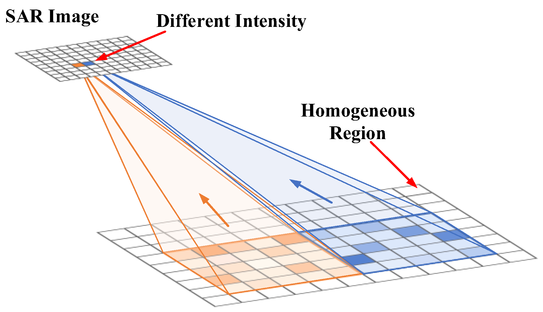
2.1.1. Principle of Speckle Noise

In the analysis of SAR imaging, three apparent causes of this granular distortion can be pointed out: propagation, antenna pattern, and the imaging process, which all result in speckle [29]. As for the effect of propagation, interference of the de-phased but coherent scattered waves after reflection and propagation results in the granular spots called speckles. Another reason for speckle is the antenna pattern which affects the antenna characteristics in the range direction. This also leads to the large correction computation in the processing systems. Finally, the special imaging process causes the speckle. In the SAR imaging process, the different amplitude spread functions combined with different phases may result in speckle imposed on the image. Speckle and signal have the same statistical properties except for the difference in power. For the single-look SAR image, its amplitude and power obey the Rayleigh distribution and the exponent distribution, respectively [30]. For a multi-look SAR image in real scenarios, the probability density function of its power is the Gamma distribution, which can be obtained by convolution of exponent distribution

$$p_{\mathit{I},N}(\mathit{I})=\frac{N^N{\mathit{I}}^{N-1}}{{\overline{\mathit{I}}}^N\mathrm{\Gamma }(N)}\exp \left(-\frac{\mathit{I}}{2{\sigma }^2}\right)$$

(1)

where $\mathit{I}$, $\overline{\mathit{I}}$, N, and σ denote the power, mean power, the number of looks, and the noise parameter, respectively, and $\mathrm{\Gamma }(\cdot )$ represents the $\mathrm{\Gamma }$ function. The principle of speckle formation in the imaging process is shown in Figure 1. The intensity of each pixel of the captured SAR image (cf. the pixel of upper rectangle in Figure 1) is jointly determined by all the scatterers within the ground resolution cell (cf. all squares representing scatterers are surrounded by a box denoting ground resolution unit). Although it is in the uniform region, the number and intensity of scatterers in each unit are random and sumless, so the intensity of adjacent pixels in the SAR image is different with each other.

Consequently, a SAR image polluted by speckle degenerates to $\mathit{I}=\mathit{U}\circ \xi$, where $\mathit{I}$ and $\xi$ represent the power of the original and speckle, and $\mathit{U}$ is the power of noise-free image. The operator of $\circ$ refers to the element-wise multiplication. The aim of de-speckling is to restore $\mathit{U}$ from $\mathit{I}$. (1) can be rewritten as

$$p_{\mathit{I},N}(\mathit{I}|\mathit{U})=\left[N^N{\mathit{I}}^{N-1}\oslash {\mathit{U}}^N\mathrm{\Gamma }(N)\right]\circ e^{-\left(N\mathit{I}\oslash \mathit{U}\right)}$$

(2)

where ⊘ denotes the element-wise division operator.

2.1.2. Total Variation Model

The TV filter [31] is also known as the Rudin–Osher–Fatemi (ROF) filter. The TV equation for a discrete image $\mathit{I}$ is

$$\mathit{I}{(x,y)}_{\mathrm{TV}}={\displaystyle \sum _{(x,y)\in \mathit{\Omega }}\left|\nabla \mathit{I}(x,y)\right|}$$

(3)

where $(x,y)$ are the pixel coordinates, $\nabla$ and $|\cdot |$ denote gradient operator and modulo operator, respectively, and $\mathit{\Omega }$ represents the domain of $\mathit{I}$. It is worth mentioning that, different from gradient operation which aims at edge detection, the gradient operator here must be difference-based for difference-based gradient reflects the intensity difference of pixels. The gradient operator is shown as

$$\nabla \mathit{I}(x,y)=\left(\begin{array}{c}\mathit{I}(x+1,y)-\mathit{I}(x,y)\\ \mathit{I}(x,y+1)-\mathit{I}(x,y)\end{array}\right)$$

(4)

because difference-based gradient reflects the true intensity difference of pixels. Then, the energy function of (3) is

$$E(\mathit{I})={\displaystyle \sum _{\mathit{\Omega }}\left|\nabla \mathit{I}\right|}$$

(5)

By letting

$$E(\mathit{I})={\displaystyle \sum _{(x,y)\in \mathit{\Omega }}{F}^{\mathrm{TV}}(x,y,\mathit{I},{\mathit{I}}_x,{\mathit{I}}_y)}$$

(6)

where $F^{\mathrm{TV}}(x,y,\mathit{I},{\mathit{I}}_x,{\mathit{I}}_y)=\sqrt{{\mathit{I}}_x^2+{\mathit{I}}_y^2}$, ${\mathit{I}}_x=\partial \mathit{I}/\partial x$, and ${\mathit{I}}_y=\partial \mathit{I}/\partial y$. The partial derivatives of $F^{\mathrm{TV}}(x,y,\mathit{I},{\mathit{I}}_x,{\mathit{I}}_y)$ can be obtained as

$$F_{\mathit{I}}^{\mathrm{TV}}=0,F_{{\mathit{I}}_x}^{\mathrm{TV}}={\mathit{I}}_x\oslash \sqrt{{\mathit{I}}_x^2+{\mathit{I}}_y^2},F_{{\mathit{I}}_y}^{\mathrm{TV}}={\mathit{I}}_y\oslash \sqrt{{\mathit{I}}_x^2+{\mathit{I}}_y^2}$$

The Euler–Lagrange equation corresponding to (5) is

$$0=-F_{\mathit{I}}^{\mathrm{TV}}+\frac{\partial }{\partial x}{F}_{{\mathit{I}}_x}^{\mathrm{TV}}+\frac{\partial }{\partial y}{F}_{{\mathit{I}}_y}^{\mathrm{TV}}=\frac{\partial ({\mathit{I}}_x\oslash \sqrt{{\mathit{I}}_x^2+{\mathit{I}}_y^2})}{\partial x}+\frac{\partial ({\mathit{I}}_y\oslash \sqrt{{\mathit{I}}_x^2+{\mathit{I}}_y^2})}{\partial y}=\nabla \cdot \left(\nabla \mathit{I}\oslash \left|\nabla \mathit{I}\right|\right)$$

(7)

Therefore, the Euler–Lagrange equation of the TV model can be expressed as

$$\mathrm{div}\left(\nabla \mathit{I}\oslash |\nabla \mathit{I}|\right)=0$$

(8)

where $\mathrm{div}(\cdot )$ is the divergence operation. TV model can form single edges during the filtration, although these edges are weak and discontinuous. In practice, TV filter can smooth the noise in homogeneous regions well. However, for $\left|\nabla \mathit{I}\right|$ in a noisy image cannot position the edges accurately, the feature protection ability of the TV filter is not satisfactory.

2.1.3. Anisotropic Diffusion Filter PDE Model

Traditional anisotropic diffusion filter is developed from the well-known Fick’s law [32]: $\nabla \cdot (\nabla f\left(\left|\nabla \mathit{I}\right|\right)\circ \nabla \mathit{I})$. To find the combination method for TV model and ADPDE model, the energy function of the ADPDE filter for a discrete image $\mathit{I}$ is given by

$$E(\mathit{I})={\displaystyle \sum _{\mathit{\Omega }}\left({\Psi }^2\ln (1/f(|\nabla \mathit{I}|))\right)}$$

(9)

where $f(|\nabla \mathit{I}|)$ is the diffusion coefficient and $\Psi >0$ denotes the fixed threshold. Specifically, the diffusion coefficient is

$$f(|\nabla \mathit{I}|)=\frac{1}{1+{(|\nabla \mathit{I}|/\Psi )}^2}$$

(10)

The higher the threshold, the weaker diffusion intensity. The relationship between the diffusion coefficient and threshold is shown in Figure 2. Accordingly, (9) can be rewritten as

$$E(\mathit{I})={\displaystyle \sum _{\mathit{\Omega }}\left\{{\Psi }^2\ln \left[1+{(|\nabla \mathit{I}|/\Psi )}^2\right]\right\}}$$

(11)

Similar to the operation of (6), let $F^{\mathrm{AD}}(x,y,\mathit{I},{\mathit{I}}_x,{\mathit{I}}_y)={\Psi }^2\ln [1+{(|\nabla \mathit{I}|/\Psi )}^2]$ here. The partial derivatives of $F^{\mathrm{AD}}(x,y,\mathit{I},{\mathit{I}}_x,{\mathit{I}}_y)$ can be organized as

$$\begin{array}{l}{F}_{\mathit{I}}^{\mathrm{AD}}=0\\ F_{{\mathit{I}}_x}^{\mathrm{AD}}=2{\mathit{I}}_x\oslash \left\{1+[({\mathit{I}}_x^2+{\mathit{I}}_y^2)/{\mathrm{\Psi }}^2]\right\}=2{\mathit{I}}_x\oslash \left[1+{(|\nabla \mathit{I}|/\Psi )}^2\right]=2{\mathit{I}}_x\circ f(|\nabla \mathit{I}|)\\ F_{{\mathit{I}}_y}^{\mathrm{AD}}=2{\mathit{I}}_y\oslash \left\{1+[({\mathit{I}}_x^2+{\mathit{I}}_y^2)/{\mathrm{\Psi }}^2]\right\}=2{\mathit{I}}_y\oslash \left[1+{(|\nabla \mathit{I}|/\Psi )}^2\right]=2{\mathit{I}}_y\circ f(|\nabla \mathit{I}|)\end{array}$$

Therefore, the Euler–Lagrange equation corresponding to (9) is

$$0=-F_{\mathit{I}}^{\mathrm{AD}}+\frac{\partial F_{{\mathit{I}}_x}^{\mathrm{AD}}}{\partial x}+\frac{\partial F_{{\mathit{I}}_y}^{\mathrm{AD}}}{\partial y}=\frac{\partial }{\partial x}({\mathit{I}}_x\circ f(|\nabla \mathit{I}|))+\frac{\partial }{\partial y}({\mathit{I}}_y\circ f(|\nabla \mathit{I}|))=\nabla \cdot (\nabla \mathit{I}\circ f(|\nabla \mathit{I}|))$$

(12)

Consequently, the Euler–Lagrange equation of anisotropic diffusion filter can be expressed as

$$\mathrm{div}[f(|\nabla \mathit{I}|)\circ \nabla \mathit{I}]=0$$

(13)

The ADPDE filter is adaptive to the pixel position, which changes from a mean filter to a high-pass filter as the pixel moves from the homogeneous region to the edge. However, the staircase phenomenon appears after ADPDE filtering in the uniform regions. Moreover, its filtering effect depends on $\Psi$, which controls the diffusion intensity.

Based on the above analysis, the TV model cannot achieve accurate feature identification, while the ADPDE model brings staircase phenomenon when dealing with homogeneous regions. Therefore, the TV model and the ADPDE model are actually complementary to each other. Moreover, the Euler–Lagrange equation inspires us to combine the two models for better filtering.

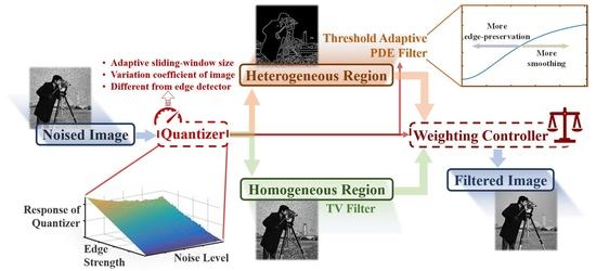
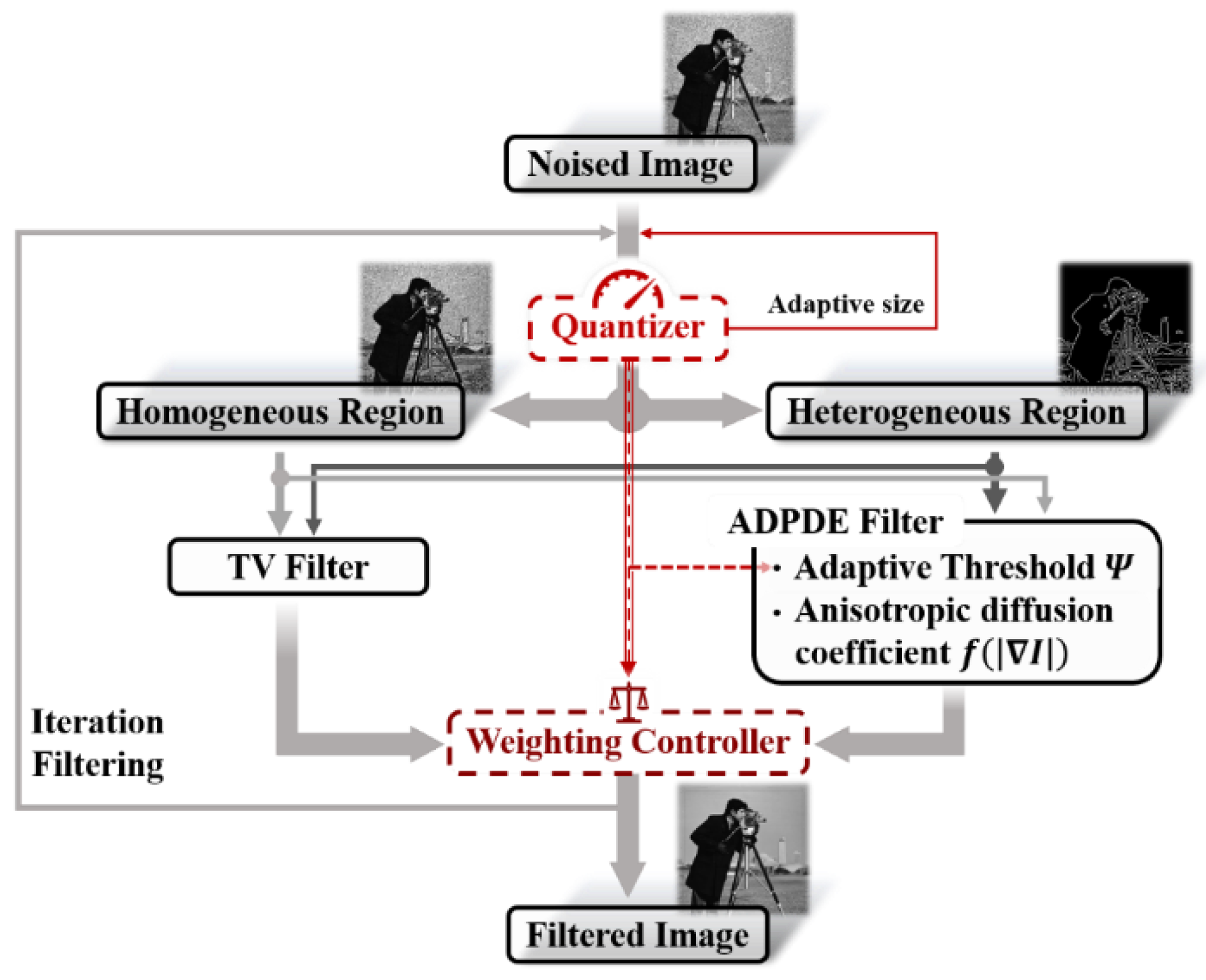
2.2. Proposed Method

An important premise of denoising is accurate feature identification, which is also a key point for the combination of TV model and ADPDE model. In order to represent features, a quantifiable representation method is proposed at the beginning. Accordingly, a quantizer is designed to not only provide the reasonable reference for the threshold $\Psi$ in (9), but also act as a weight controller between the TV and the ADPDE model, resulting in better denoising and edge-preservation. Then, the threshold adaptive ADPDE model and the combination model of TV and ADPDE equipped with the weight controller are introduced.

2.2.1. Pixel Position Quantizer

Conventionally, the edge detectors obtain binarization results stably to distinguish edges. The rationale for this is that the responses of ideal edge detection operators in homogeneous and heterogeneous regions are very different, regardless of the noise intensity. However, the quantizer in this paper aims to represent the positional properties of pixels continuously, which helps to control the diffusion process.

The variation coefficient (VC) has been chosen as the input of quantizer. That is because the VC is not bound by of measurement scale and dimension to describe the dispersion degree of various data [4,26], and the VC is defined as

$$v_c^{\mathbb{W}}=\frac{\sigma }{\mu }$$

(14)

where $\sigma$ and $\mu$ represent the standard deviation and mean value, and $\mathbb{W}$ is the data source. The larger the VC is, the more discrete the data is. Combined with a zero-crossing filter, the ratio of $v_c^{{\mathbb{W}}_1}$ and mean $v_c^{{\mathbb{W}}_1}$ in the concentric window ${\mathbb{W}}_2$, is regarded as the numerical value for the quantization indicator. If the length of ${\mathbb{W}}_1$ and ${\mathbb{W}}_2$ are $d_1$ and $d_2$, respectively, we make $d_2\ge 3d_1$. Specifically, the quantizer is defined as

$$q_i(x,y)={\left[\frac{v_c^{{\mathbb{W}}_1}(x,y)}{{\displaystyle {\sum }_{{\mathbb{W}}_2}{v}_c^{{\mathbb{W}}_1}(x,y)/\left|{\mathbb{W}}_2\right|}}\right]}^{0+}$$

(15)

where ${[\cdot ]}^{0+}$ denotes the zero-crossing filter. The denominator in (15) is the average of $v_c^{\mathbb{W}}$, which represents the mean dispersion in ${\mathbb{W}}_2$. The result q_i is larger in heterogeneous regions and smaller in homogeneous regions. Moreover, to overcome the quantizer’s dependence on the window size, the size of sub-window ${\mathbb{W}}_1$ is defined as

$$d_1=\{\begin{array}{l}\min [d_1+2,d_{1,\max }],\mathrm{if}{v}_c^{{\mathbb{W}}^{\prime }}\le T_1\\ \max [d_1-2,d_{1,\min }],\mathrm{if}{v}_c^{{\mathbb{W}}^{\prime }}>T_1\end{array}$$

(16)

where ${\mathbb{W}}^{\prime }$ represents the pixels around the border of ${\mathbb{W}}_1$, and $d_{1,\min }$ and $d_{1,\max }$ are the size limit for ${\mathbb{W}}_1$. The window side has an impact on the proposed quantizer; smaller $d_{1,\min }$ or larger $d_{1,\max }$ makes quantizer more sensitive to noise, while larger $d_{1,\min }$ or smaller $d_{1,\max }$ will produce the opposite effect and lose the distinguishability to features (we predefined $d_{1,\min }=3$ and $d_{1,\max }=11$ empirically in this paper). $T_1$ is a threshold obtained by

$$T_1=\left(1+\sqrt{\frac{1+2{\sigma }^2}{\left|{\mathbb{W}}^{\prime }\right|-1}}\right)\cdot \sigma$$

(17)

The schematic diagram of size adaptive window is shown in Figure 3. The experiment results regarding the quantizer’s performance are shown in Section 3.1.

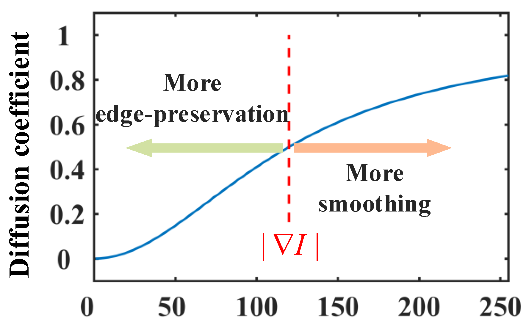
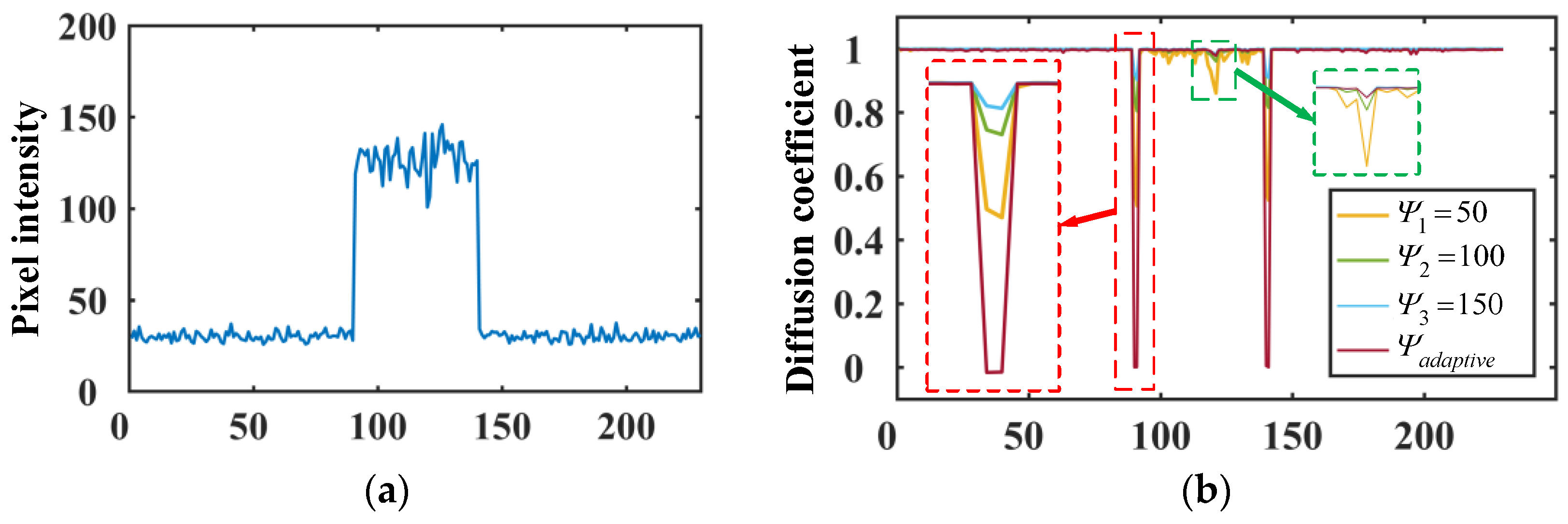
2.2.2. Threshold Adaptive ADPDE Model

So far, a stable pixel position quantizer with a dynamic response based on VC has been proposed. We adopt it here to control the threshold in (10) to enhance edge-preserving ability of the ADPDE method. The adaptive threshold ${\Psi }_{\mathrm{AT}}$ at $(x,y)$ is obtained by

$${\mathit{\Psi }}_{\mathrm{AT}}(x,y)=|\nabla \mathit{I}(x,y)|\cdot a^{q_i(x,y)-b}$$

(18)

where $a\in (0,1)$ and $b\in (-\infty ,0]$ are the hyperparameters. An example for the effect of Ψ_AT on diffusion coefficient is shown in Figure 4. Accordingly, it can be seen that the diffusion coefficient obtained by (10) with the proposed adaptive threshold brings the weakest diffusion intensity, which means the best feature preservation.

Due to the adaptive threshold, the diffusion intensity in ADPDE model decreases more at the sharper edges to keep the image feature. The diffusion coefficient is represented as $f_{\mathrm{AT}}(|\nabla \mathit{I}|)$. Accordingly, the threshold-adaptive ADPDE can be modeled as

$$\frac{\partial \mathit{I}(x,y)}{\partial t}=\mathrm{div}\left\{|\nabla \mathit{I}(x,y)|/[1+{(|\nabla \mathit{I}(x,y)|/{\Psi }_{\mathrm{AT}}(x,y))}^2]\right\}$$

(19)

By using the gradient descent method, the final solution of the threshold-adaptive ADPDE model can be expressed as

$$\{\begin{array}{l}{\mathit{I}}_{n+1}(x,y)={\mathit{I}}_n+\Delta t\cdot \mathrm{div}\left\{|\nabla \mathit{I}(x,y)|/[1+{(|\nabla \mathit{I}(x,y)|/{\Psi }_{\mathrm{AT}}(x,y))}^2]\right\}\\ {\mathit{I}}_0(x,y)=\mathit{I}(x,y)\end{array}$$

(20)

where $\Delta t$ represents the step-size.

We summarize the threshold-adaptive ADPDE algorithm in Algorithm 1.

Algorithm 1 Threshold adaptive ADPDE filter

Input: The noised image ${\mathit{I}}_0$, iteration times $n$, step size $\Delta t$ for iteration.

Output: The filtered image $\mathit{I}$.

Initialize:$i=1$,$a\in (0,1)$,$b\in (-\infty ,0]$.

Begin

1: for $i\le n$ do

2:        Obtain the magnitude $|\nabla {\mathit{I}}_{i-1}|$ of image ${\mathit{I}}_{i-1}$;

3:        Obtain the quantizer response $q_{i-1}$ on ${\mathit{I}}_{i-1}$ by (15);

4:        Calculate the adaptive threshold ${\mathit{\Psi }}_{\mathrm{AT}}^{i-1}$ for every pixel by (18);

5:        Get the diffusion coefficient $f_{\mathrm{AT}}(|\nabla {\mathit{I}}_{i-1}|)$ by (10);

6:        Generate the new image result ${\mathit{I}}_i$ by gradient descent method in (20).

10:        $i=i+1$;

11: end

12: The output image $\mathit{I}={\mathit{I}}_n$;

End

2.2.3. Combination Model of TV and ADPDE

By integrating the advantages of the TV model and the threshold-adaptive ADPDE model, better filtering results can be achieved. According to (8) and (13), the combination model can be expressed as

$$\frac{\partial \mathit{I}}{\partial t}={\mathit{S}}_w\circ \mathrm{div}(f_{\mathrm{AT}}(|\nabla \mathit{I}|)\circ \nabla \mathit{I})+\left(1-{\mathit{S}}_w\right)\circ \mathrm{div}\left(\nabla \mathit{I}\oslash |\nabla \mathit{I}|\right)$$

(21)

where ${\mathit{S}}_w$ is regarded as a switching controller, which the aforementioned quantizer is embedded in, to realize the automatic switchover between TV and ADPDE models. ${\mathit{S}}_w$ is defined as

$${\mathit{S}}_w(x\text{,}y)=e^{\left(\frac{-1}{q\left(x\text{,}y\right)}\right)}$$

(22)

In the homogeneous areas, the novel model emphasizes the role of the second term on the left of (21). In this case, $q_i(x,y)$ would be small. Therefore, the strong diffusion will smooth more there, which in turn is conductive to more effective noise suppression. In the heterogeneous areas, the role of the first term on the left of (21) will be highlighted. The features can be preserved effectively.

For more details, the Euler–Lagrange equations of TV and ADPDE can be rewritten as

$$\mathrm{div}\left(\nabla \mathit{I}\oslash |\nabla \mathit{I}|\right)=\left({\mathit{I}}_x^2\circ {\mathit{I}}_{\mathrm{yy}}-2{\mathit{I}}_x\circ {\mathit{I}}_y\circ {\mathit{I}}_{\mathrm{xy}}+{\mathit{I}}_y^2\circ {\mathit{I}}_{\mathrm{xx}}\right)\oslash \sqrt{{({\mathit{I}}_x^2+{\mathit{I}}_y^2)}^3}$$

(23)

and

$$\begin{array}{ll}\mathrm{div}(f_{\mathrm{AT}}& (|\nabla \mathit{I}|)\circ \nabla \mathit{I})=({\mathit{\Psi }}_{\mathrm{AT}}^2\circ {\mathit{I}}_{\mathit{xx}}+{\mathit{\Psi }}_{\mathrm{AT}}^2\circ {\mathit{I}}_{\mathit{yy}}-{\mathit{I}}_x^2\circ {\mathit{I}}_{\mathit{xx}}+{\mathit{I}}_y^2\circ {\mathit{I}}_{\mathit{xx}}\\ & -4{\mathit{I}}_x\circ {\mathit{I}}_y\circ {\mathit{I}}_{\mathit{xy}}+{\mathit{I}}_x^2\circ {\mathit{I}}_{\mathit{yy}}-{\mathit{I}}_y^2\circ {\mathit{I}}_{\mathit{yy}})/{\left[\left({\mathit{\Psi }}_{\mathrm{AT}}^2+{\mathit{I}}_x^2+{\mathit{I}}_y^2\right)\oslash {\mathit{\Psi }}_{\mathrm{AT}}\right]}^2\end{array}$$

(24)

where ${\mathit{I}}_{xx}={\partial }^2\mathit{I}/\partial x^2$, ${\mathit{I}}_{yy}={\partial }^2\mathit{I}/\partial y^2$, and ${\mathit{I}}_{xy}={\partial }^2\mathit{I}/\partial xy$.

In general, the quantizer proposed in this paper acts as the weighting controller between TV and ADPDE models, and the controller of diffusion intensity in the ADPDE model. An overview of proposed denoising method is shown in Figure 5, and here we name our method quantitative anisotropic diffusion (QAD) filter.

3. Results

In this section, the feature positioning accuracy and dynamic response capability of the proposed quantizer have been verified firstly. To demonstrate the effectiveness and robustness of the proposed QAD filter, we applied it to a synthetic dataset and natural datasets with different systems and different bands. All the datasets were converted to the single-look matrix format, without a multi-look operation.

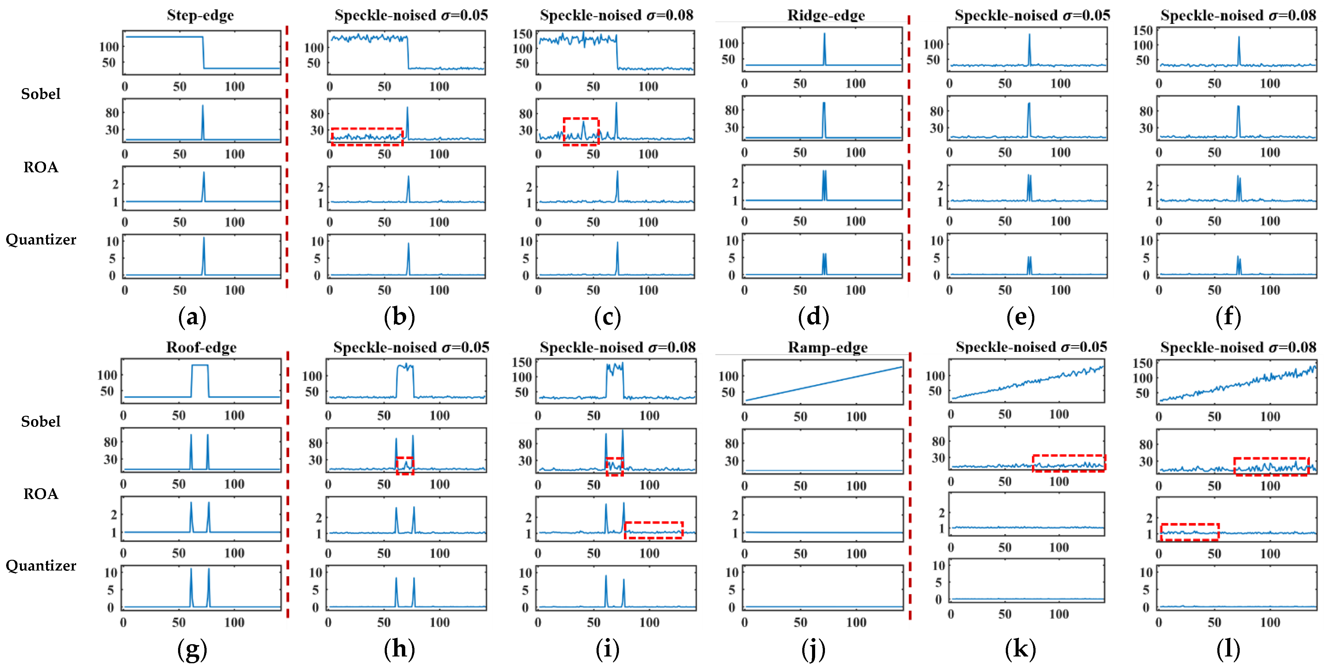
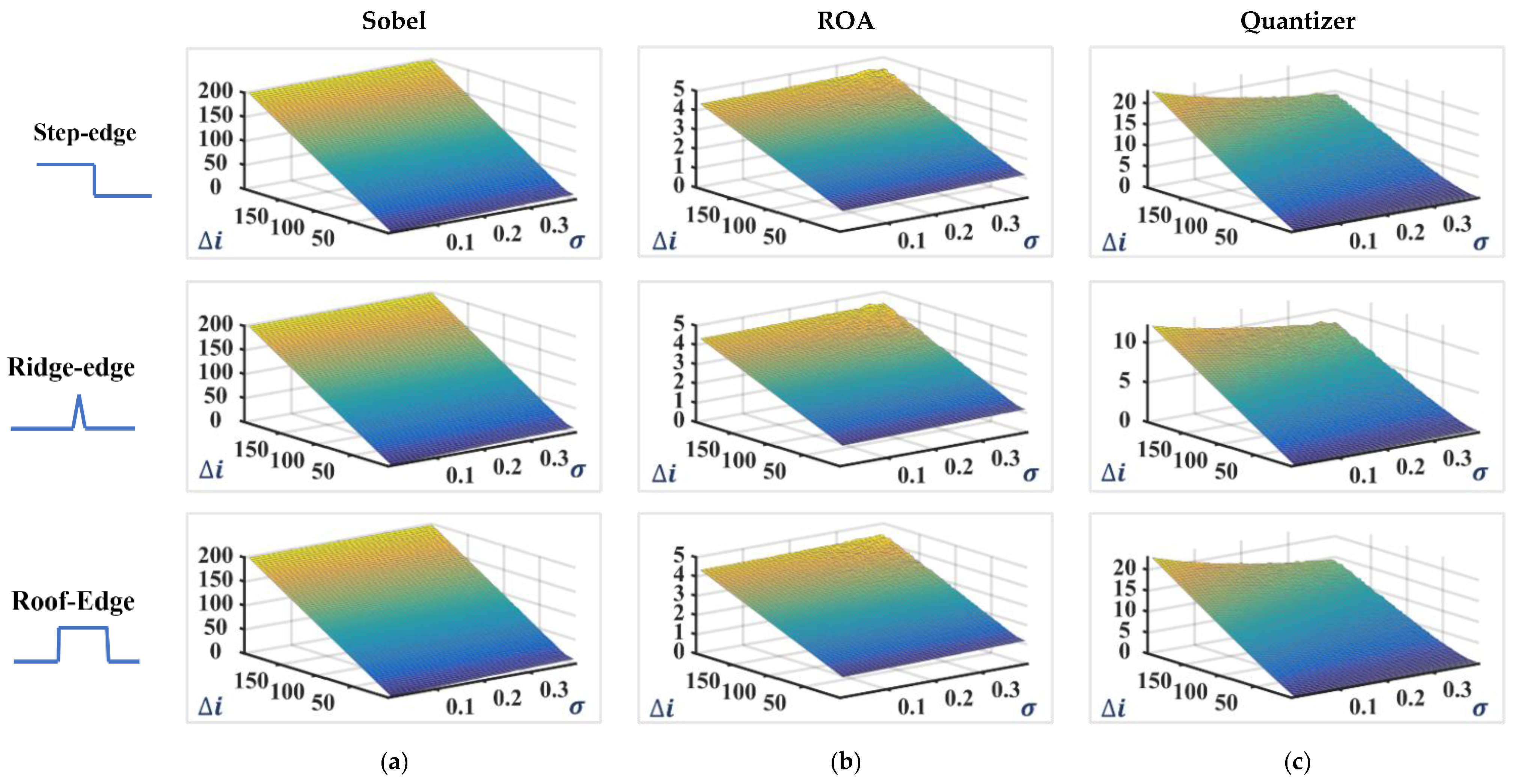
3.1. Monte Carlo Simulations for the Quantizer

Firstly, in order to confirm the edge positioning accuracy of proposed quantizer, we compare the edge response of some comparative methods. Conventional edge detector responds differently in heterogeneous and homogeneous areas, and the classical detection method is gradient-based or ratio-based. Sobel detector [6] and ratio of average (ROA) [7] detector are the typical gradient-based and ratio-based methods, respectively. For a 1-D signal $s$, the Sobel detector can be rewritten as

$$q_{\mathrm{Sobel}}=\mathrm{abs}\left[s\right(x+1)-s(x\left)\right]$$

(25)

The 1-D ROA detector can be written as

$$q_{\mathrm{ROA}}=\max (\frac{M(s(x-r:x))}{M(s(x:x+r))},\frac{M(s(x:x+r))}{M(s(x-r:x))})$$

(26)

where $M(\cdot )$ is mean operation and $r$ represents the radius of ROA detector. Here we set $r=2$, tentatively. Various edge-like synthetic 1-D signals are selected to test the responses of different approaches. We choose the step-, pulse-, square-, and slope-signal to denote the step-, ridge-, roof-, and ramp-like edges respectively. Detection results are displayed in Figure 6. Note that a deviation of one pixel is allowed while detecting ridge-like edge. That is because both sides of the ridge are steep enough to be recognized as edges. Due to the multiplicative property of speckle noise, the disturbance caused by speckle grows larger while signal intensity is higher. It results in more errors generated from the Sobel detector, which are shown in Figure 6b,c,h,i,k,l. The ROA detector performs unstably both in high-intensity regions and nearby the edges, which is pointed out in Figure 6i,l. Conversely, the proposed quantizer can respond precisely to edges with or without speckle.

Secondly, a series of Monte Carlo experiments are carried out to prove the dynamic response capability of the proposed quantizer. In the experiments, step signal, pulse signal, and square signal are used to represent the step-edge, ridge-edge, and roof-edge, and the intensity difference Δ_i of these signals at the edge position ranges from 0 to 200 with interval 2.5. To simulate a noisy situation, speckle noise is injected, whose σ changes from 0 to 0.4 with an interval of 0.01. This results in 3200 test groups and 500 Monte Carlo simulations are conducted in every test group.

The results of Monte Carlo experiments are shown in Figure 7. The proposed quantizer response grows as $\Delta i$ increases, so do Sobel and ROA detector. However, the noise at edges needs to be more thoroughly filtered when the noise is stronger. Otherwise, the remaining noises would still affect the denoising result. It can be seen that Sobel and ROA detectors respond stably as noise increases, which means that these edge detectors always preserve the noise at edges as shown in Figure 7a,b. Note that the smooth surface of Sobel detector results from the averaging of Monte Carlo experiments. In fact, the result of the Sobel detector is unstable. In conclusion, the proposed quantizer can respond according to both $\Delta i$ and $\sigma$, which can adjust diffusion process to keep the features and denoise as can be seen from Figure 7c.

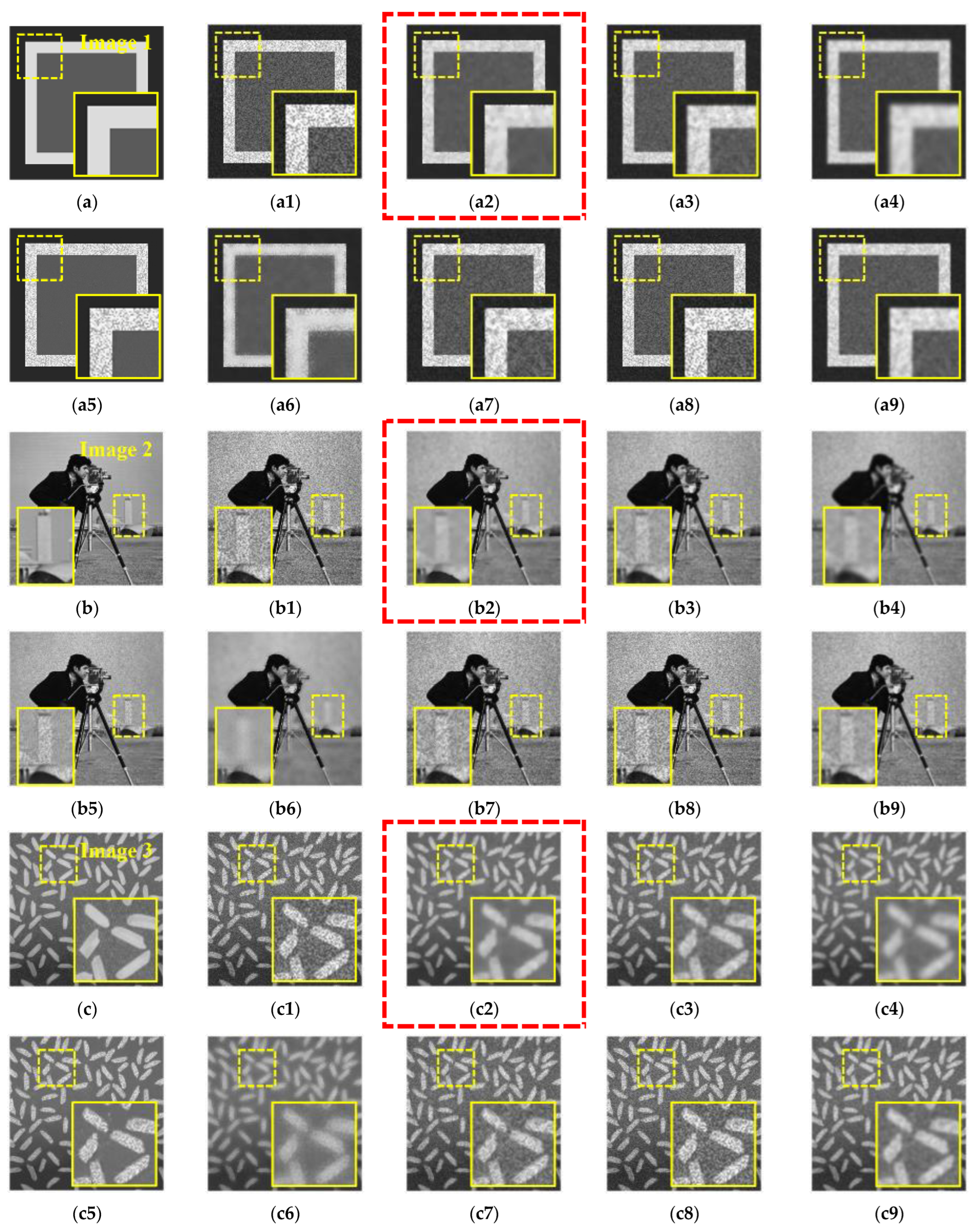
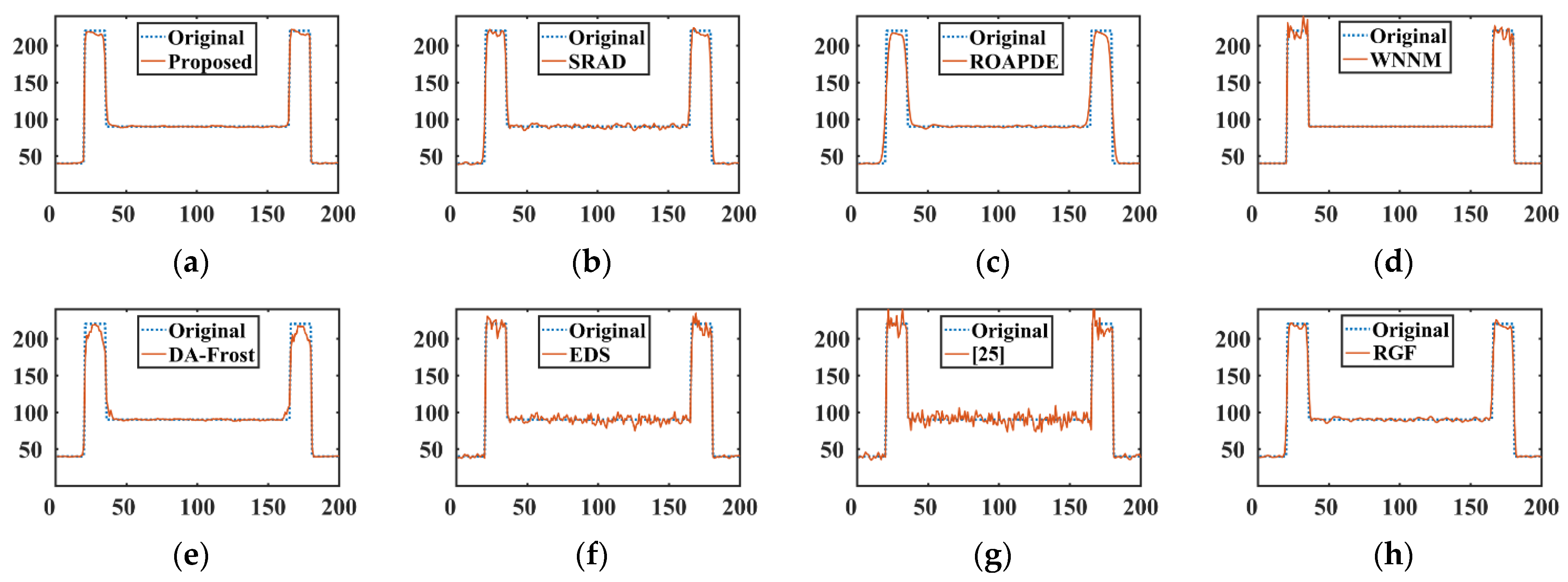
3.2. Speckle Suppression on Synthetic Images

In this subsection, we conduct extensive experiments on image denoising to verify the effectiveness of the proposed method. We compared our algorithm (QAD) with two kinds of filters. One kind of filters belong to the category of the PDE-based filters, such as SRAD [17] and ROAPDE, which uses ROA edge detector to guide diffusion filtering. The other kind of methods are advanced at present, such as the weighted nuclear norm minimization filter (WNNM) [28], the double adaptive Frost filter (DA-Frost) [14], enhanced directional smoothing filter (EDS) [26], recurrent guidance filter (RGF) [27] and the method in [25]. Note that the method in [25] can de-speckle, which has been proved by authors. The source codes of most competing methods are obtained from the original authors and we used the default parameter settings. The experimental results of speckle suppression on synthetic images are shown in Figure 8. Due to limited space, please enlarge the tables and figures on the screen for better comparison. To evaluate the quality of the recovered images, equivalent number of looks, peak signal-to-noise ratio, and structure similarity index measure metrics are used, and their mathematical expressions are shown in

Table 1. Evaluation indexes for images.

Index	Formula	Parameters
Equivalent number of looks (ENL) [33]	$\mathrm{ENL}=\frac{{\mu }^2}{{\sigma }^2}$	μ-Intensity average of image σ-Intensity variance of image
Peak signal-to-noise ratio (PSNR) [34]	$\mathrm{PSNR}=20\log \left(\frac{\mathrm{Max}}{\mathrm{MSE}}\right)$	Max-The maximum intensity of the image MSE- Mean square error [34]
Structure similarity index measure (SSIM) [35]	$\mathrm{SSIM}=\frac{(2\mu ’\mu +C_1)(2\sigma ’\sigma +C_2)}{(\mu {’}^2+{\mu }^2+C_1)(\sigma {’}^2+{\sigma }^2+C_2)}$	C1, C2-Two constants to avoid the denominator being zero. We set C1 = 6.5025 and C2 = 58.5225 in this paper.

. In addition, the greater ENL means the better visual effects of the denoising algorithm; the larger PSNR shows the denoising algorithm ability is stronger; and the SSIM closer to 1 means the image has better quality.

We firstly use all methods to conduct the speckle suppression experiments on some synthetic images. On the one hand, in order to verify the de-noising effect of real SAR images, we manually draw a rectangular frame simulation to simulate the single building in SAR images. On the other hand, classical optical images are used as simulation diagrams to test the robustness of different methods to deal with complex image situations. The speckle noise with standard deviation of 0.03 is added to the synthetic image set uniformly.

The parameters $(a,b,d_{1,\min },d_{1,\max })$ in the proposed QAD filter are set to $(0.005,-1.5,3,11)$. Moreover, the PDE-based methods iterate uniformly for 160 times with $\Delta t=0.01$ for de-speckling. The experimental results of the synthetic image set are shown in Figure 6. The indicators of all the simulation results are recorded in

Table 2. Indexes of simulation images.

Image	Index	QAD	SRAD	ROAPDE	WNNM	DA-Frost	EDS	Method in [25]	RGF
1	ENL	1148.208	188.8266	788.4655	2456.825	732.6817	47.5501	19.5870	265.1043
	PSNR	28.3762	24.4482	21.7142	25.3275	24.3889	22.5461	19.3740	24.3943
	SSIM	0.9920	0.9794	0.9593	0.9789	0.9791	0.9698	0.9392	0.9792
2	ENL	173.7292	72.0986	124.7040	170.5701	187.0147	35.7569	18.8991	79.6633
	PSNR	26.9975	25.5037	22.6524	26.9237	25.9660	23.7714	20.7938	25.3325
	SSIM	0.9832	0.9761	0.9519	0.9834	0.9786	0.9662	0.9362	0.9751
3	ENL	127.1609	77.2870	123.3472	81.7275	160.5184	45.4357	20.2846	86.8317
	PSNR	25.4831	26.0161	23.6909	25.8179	22.2074	23.1071	19.9500	25.9086
	SSIM	0.9748	0.9602	0.9447	0.9628	0.9181	0.9447	0.8970	0.9693

.

From the objective evaluation criteria shown in Table 2, it can be observed that the proposed QAD filter can keep the structure information of the image better, which makes the SSIM of QAD higher than others. Meanwhile, one can observe that the proposed QAD filter outperforms other competing methods in most cases in terms of ENL and PSNR. For image 1, the ENLs of QAD over SRAD, ROAPDE, DA-Frost, EDS, method in [25] and RGF are as much as 959.3814, 359.7425, 415.5263, 1100.658, 1128.621, 883.1037, respectively. In terms of image 2, the ENLs of QAD over SRAD, ROAPDE, WNNM, EDS, method in [25] and RGF are as much as 101.6306, 49.0252, 3.1591, 137.9723, 154.8301, and 94.0659, respectively. As for image 3, the ENLs of QAD are 49.8739, 3.8137, 81.7252, 106.8763, 40.3292 higher than SRAD, ROAPDE, WNNM, EDS, method in [25] and RGF. In terms of PSNR, it can be seen that the proposed QAD can also achieve better performance than other competing methods in most cases. The only exception is in image 3 for which there are many features to protect, resulting in PSNR of QAD being suboptimal. Nonetheless, the result of QAD still obtains better ENL and SSIM. The WNNM can better suppress speckle in dark regions, which is the reason that the ENL of WNNM is larger than QAD in image 1. There still is noticeable residual speckle in bright regions after WNNM filtering as shown in Figure 8(b5,c5), so that its ENL is less than QAD for image 2 and 3. The theoretical reason is that WNNM method reduces the singular values of image matrix in different weight but same number, leading the number of singular values in bright regions to be more than that in dark regions.

Another Monte Carlo comparative experiment is conducted to demonstrate the superiority of QAD method. We added speckle noise to three simulation images, and then applied the denoising methods mentioned above. After experiments, a row of pixels is selected arbitrarily in each result image to compare with that of the original image to demonstrate the image restoration ability of different methods. The comparison results are shown in Figure 9, Figure 10 and Figure 11, respectively. As shown in Figure 9d, WNNM fails in the high-intensity region while effectively removes the noise in the low-intensity homogeneous region. EDS and method in [25] remain the clutter obviously. ROAPDE and DA-Frost methods blur the edge seriously, which leads to the fuzzy features in the image. It seems that SRAD and RGF perform as well as the proposed method, but we can still find out the fine intensity fluctuations in Figure 9b,h are more evident than Figure 9a. That indicates proposed QAD method has better filtering ability. Similar to Figure 9, the proposed QAD method makes a balance between denoising and feature preservation in Figure 10. The second synthetic image has some narrow inconspicuous features with low intensity. It can be seen from Figure 10 that almost all methods blur them. However, the proposed QAD method keeps both the wide low-intensity and the narrow high-intensity features subtly, as shown in Figure 10a. There are many clutters in the third original synthetic image, as the blue curve shows in Figure 11. Most of the filtering methods blur them. It is worth paying attention to the restorations for predominant features by various methods. As shown in Figure 11d, the result of WNNM seems to be the best. However, almost no change can be found from the filtering result of method in [25], which can be verified by Figure 11g. Figure 11a shows that the proposed QAD method protects the features with various widths very well. In general, the 1-D results of proposed QAD method are closest to original data.

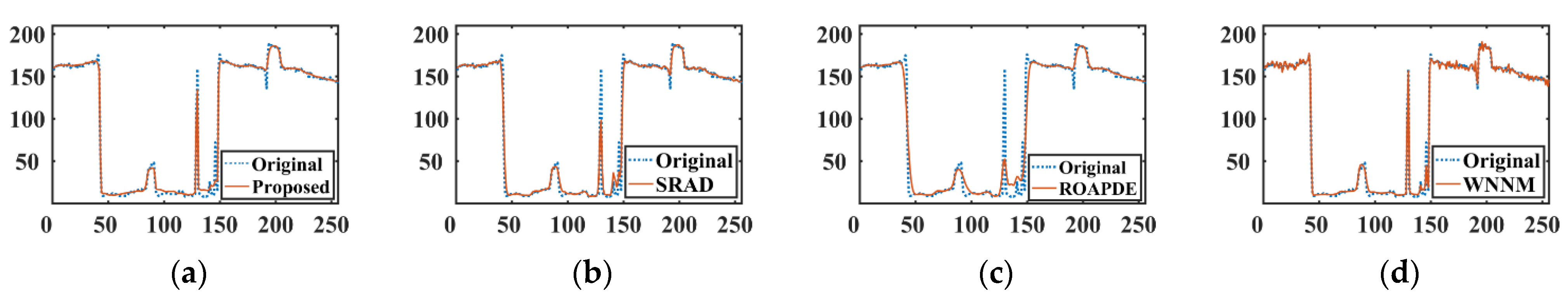
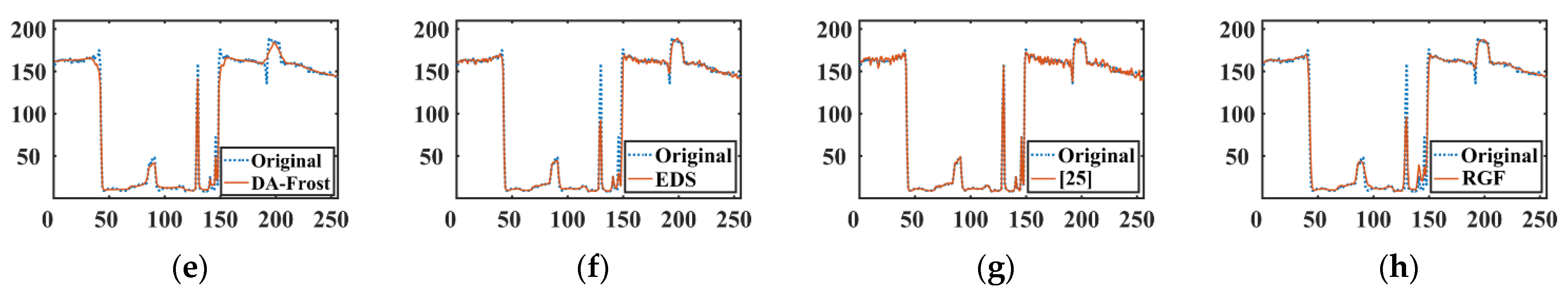
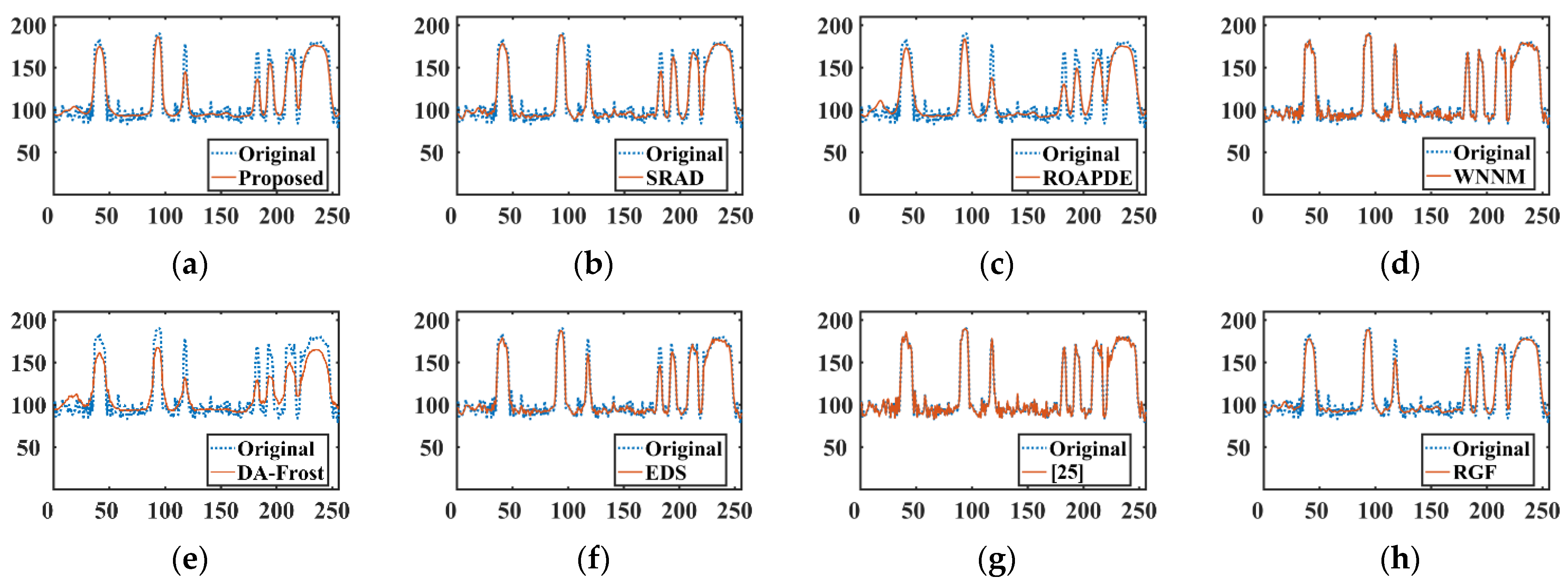
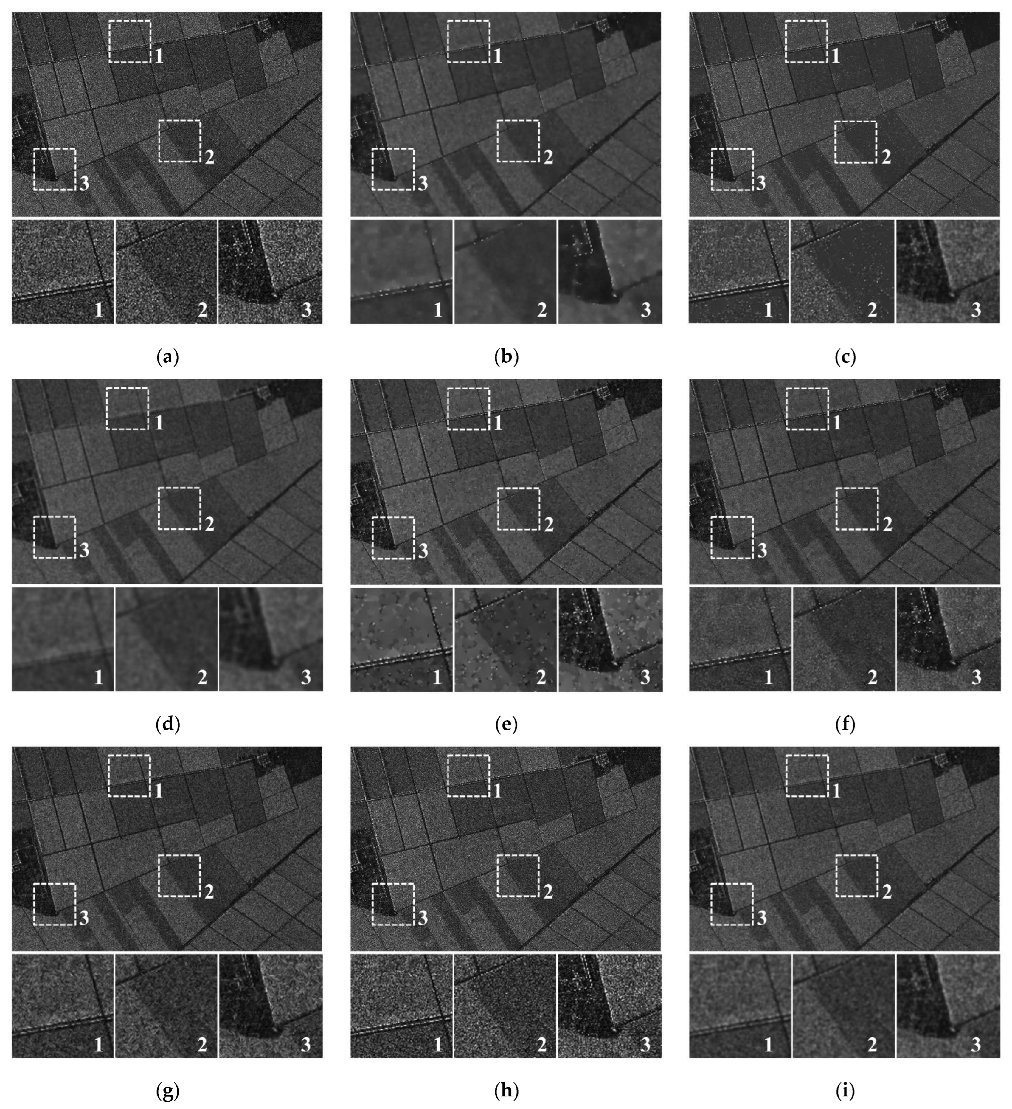
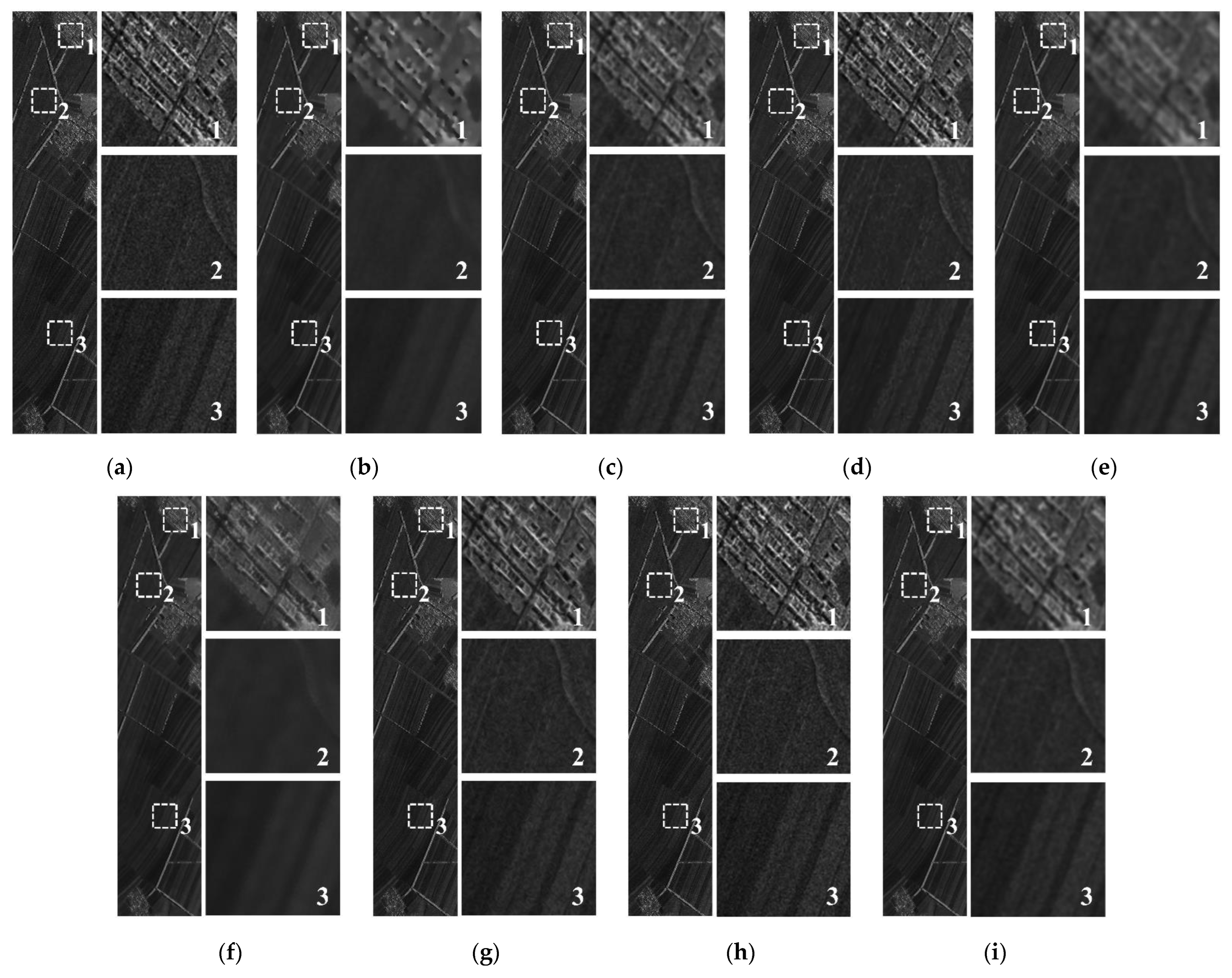
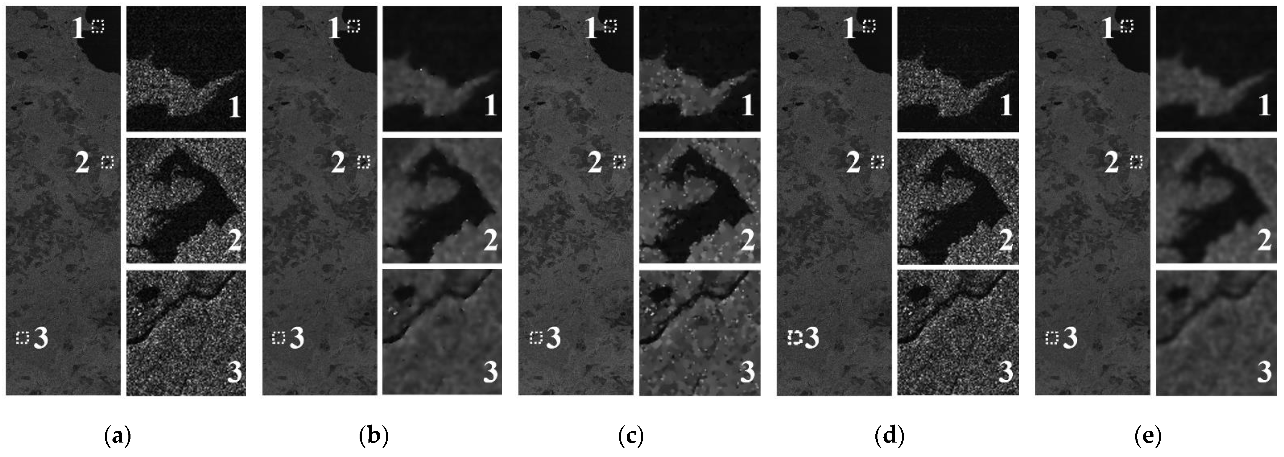
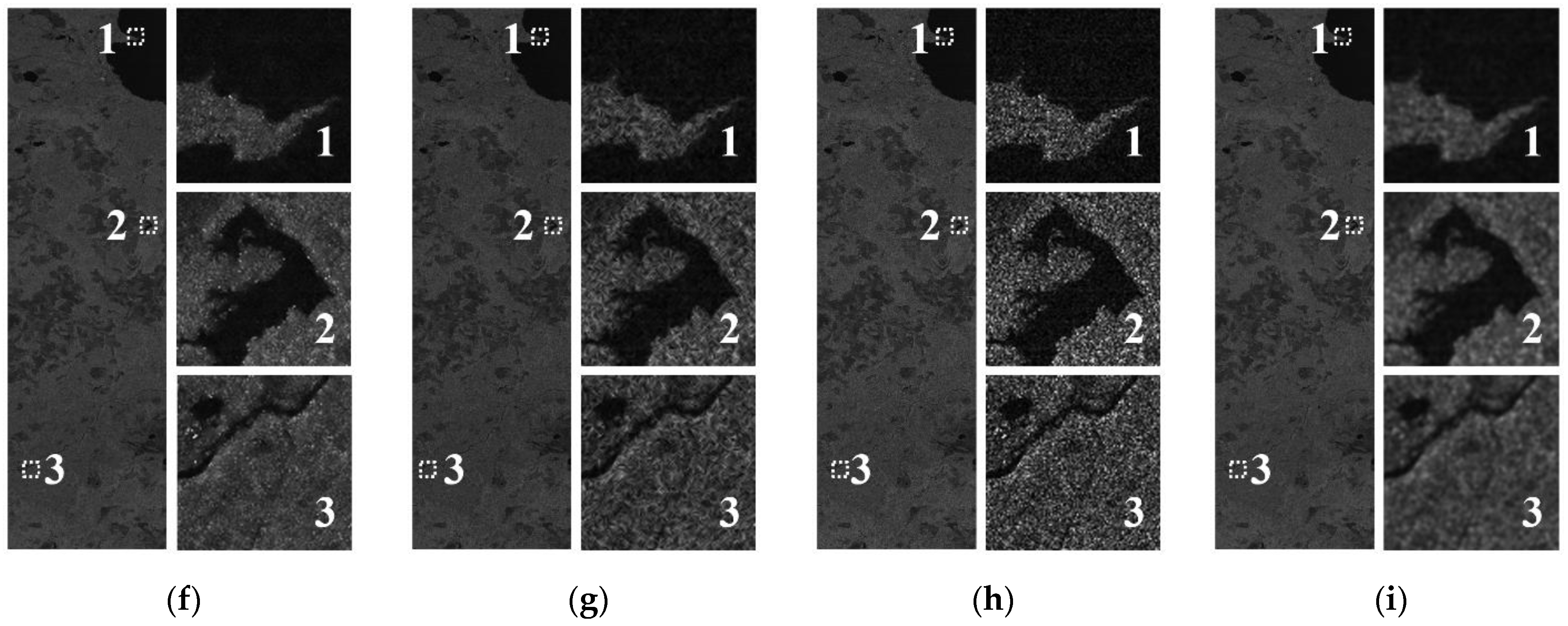
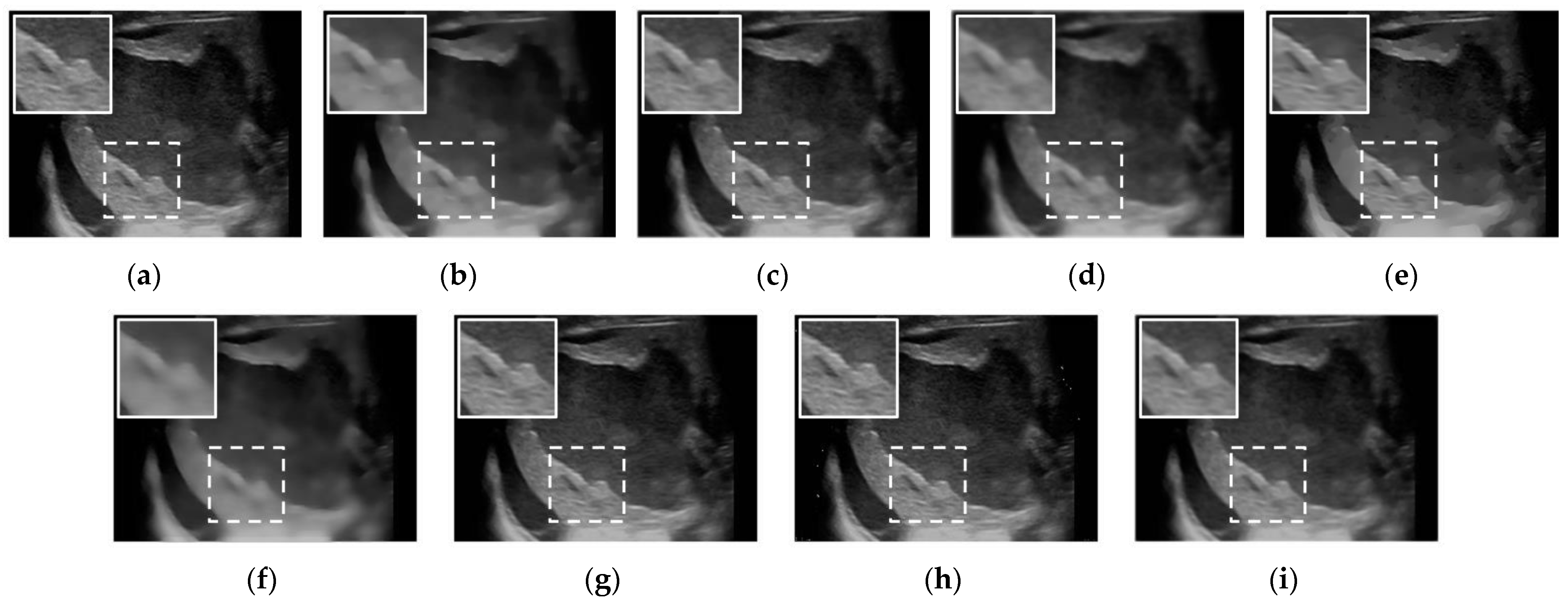
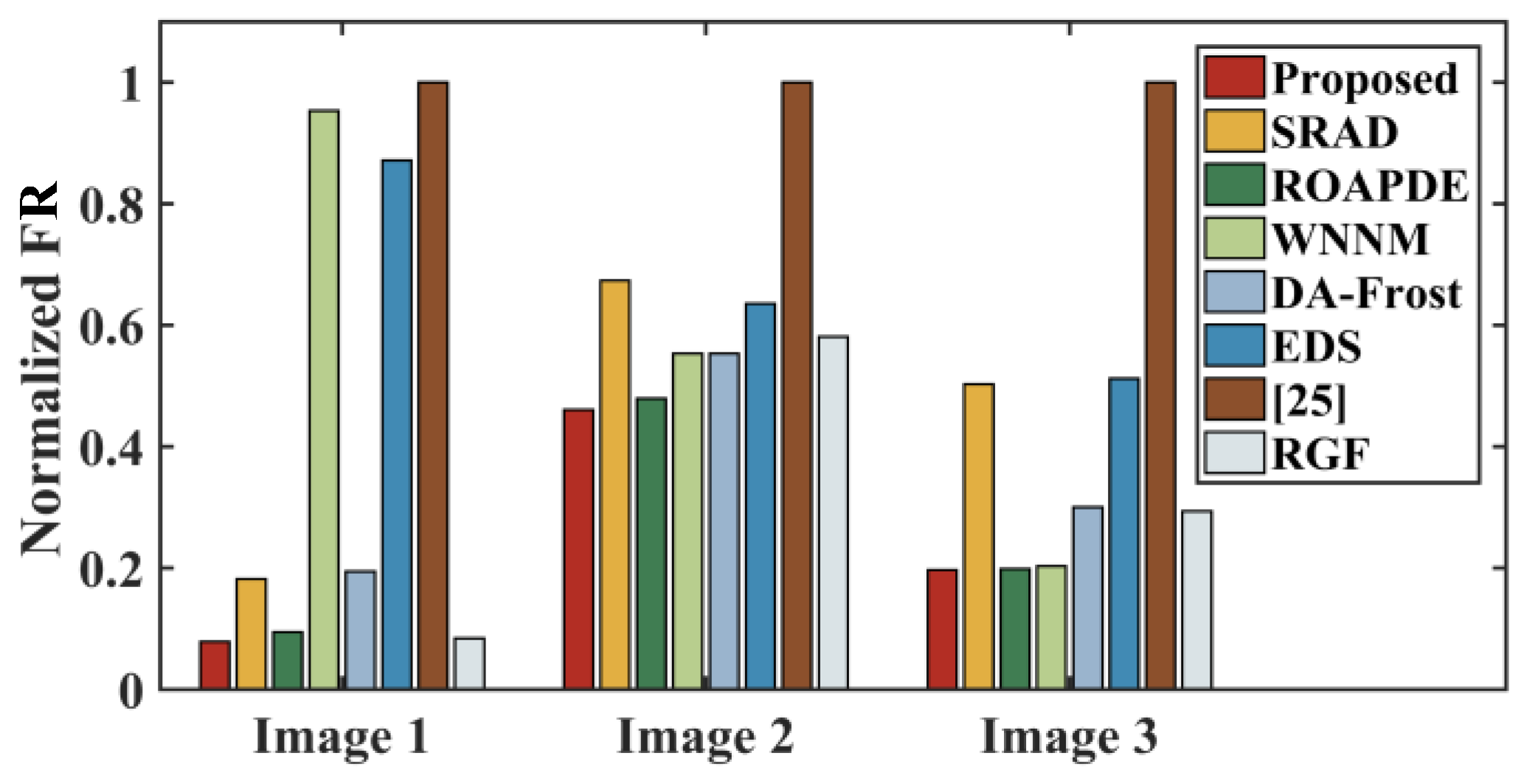
3.3. Speckle Suppression on Natural Images

In this subsection, three natural SAR images are used as datasets for speckle suppression. The first dataset is X-band high-resolution airborne SAR data from Liaoning, China. A region of 788 × 520 pixels was selected, where dark areas, bright areas, and vegetation with rich boundaries are included. The second dataset is also high-resolution airborne SAR data from Liaoning, China, but it is S-band and 402 × 2000 in size. The S-band SAR image contains many buildings and farmlands with rich homogenous regions, edges, and dark areas. The third dataset is GF-3 C-band high-resolution spaceborne SAR data in Russia, whose size is 1314 × 4471. The SAR datasets are supported by the Aerospace Information Research Institute, Chinese Academy of Sciences and China Centre for Resources Satellite Data and Application. The experimental results show that the proposed QAD method achieves good results on high-resolution images in X-, S-, and C-bands images, which proves the robustness of the QAD. The original X-, S-, and C-bands images are shown in Figure 12a, Figure 13a and Figure 14a, respectively.

Due to low flight altitude, the speckle noise is more noticeable and stronger in airborne SAR images. By contrast, the spaceborne SAR image is less noisy. Therefore, the de-speckling goals of airborne image and spaceborne image are different. A stronger denoising process is needed in airborne images while better feature preservation is required in spaceborne images. More experimental results of airborne SAR images and spaceborne SAR image are shown in Figure 12, Figure 13 and Figure 14, respectively. For better visualization of the results, we selected three small scenes from X-band, S-band, C-band, and ultrasound images to compare the detail preservation and speckle suppression. ENLs of all regions are recorded in

Table 3. ENLs of regions in Figure 11 and Figure 12.

Image	Region	Original	QAD	SRAD	ROAPDE	WNNM	DA-Frost	EDS	Method in [25]	RGF
X-band	Region 1	3.7552	78.9749	28.6375	77.1546	6.3818	18.7063	9.8756	3.7607	33.3181
	Region 2	3.1325	30.8681	17.3108	30.3656	8.2419	11.6715	7.6006	3.1375	19.3260
	Region 3	1.9163	7.1138	6.3428	8.9477	3.0102	4.1101	3.6157	1.9189	6.7453
S-band	Region 1	3.4429	8.4866	7.3068	12.9362	3.5752	9.2775	4.7948	3.4463	7.9731
	Region 2	14.0738	70.1042	29.4621	44.3013	24.6344	66.3731	22.2277	14.1087	31.4164
	Region 3	14.5170	39.8835	27.0439	33.2399	24.8324	39.2225	21.5914	14.5341	28.2677
C-band	Region 1	0.8809	1.7718	1.6442	1.8236	0.9461	1.5046	1.4087	0.8819	1.6997
	Region 2	1.4821	4.2169	3.8279	4.2096	1.5261	3.1057	2.6813	1.4843	4.0827
	Region 3	2.2523	13.2380	10.4906	21.9790	2.3085	6.8664	5.0904	2.2554	12.5298

.

Figure 12 covers a wide area of fields, each of which is considered homogeneous internally. As such, denoising assignment for Figure 12a is aimed at smoothing the interior of each farmland and preserving the boundaries clearly. As can be seen from Figure 12a, there is something with high reflectance at the boundary of some fields, which should be protected as far as possible for better feature preservation. The result of ROAPDE, as Figure 12d shows, is inferior because the strong reflection features at the boundary are lost. Referring to Table 3, the proposed QAD has the best filtering effect, which means better performance in both denoising and detail preservation, on the X-band SAR image in this paper, as shown in Figure 12b. These phenomena can also be observed in Figure 13b and Figure 14b. Figure 13a shows the suburban area. It contains a concentration of buildings and a lot of farmlands. The ROAPDE method holds strong smoothing capabilities, but it tends to over-blur borders and outlines of buildings as is shown by Figure 13d and Figure 14d, which is also the reason that ENLs of ROAPDE are larger than most comparing methods. It can be concluded that the ROA edge detector fails to extract the edges in SAR images and simply embedding an edge detector into PDE filter has no obvious effect. Combining with the ENLs in Table 3, we can conclude that the proposed QAD method has achieved the most satisfactory suppression result.

Figure 14 covers a large area of ground scene, which contains many indistinguishable ground targets. Therefore, in the de-noising processing of this space-borne C-band SAR image, attention should be paid to protecting the terrain profiles and smoothing the uniform areas. For this particular figure, many methods fail to remove speckle noise—such as SRAD, ROAPDE, DA-Frost, EDS, method in [25]—and RGF, as can be seen from obvious speckles in Figure 14c,d,f–i. Figure 14e shows that the WNNM method over-smooths the edges resulting in low-identification of features. The proposed QAD method filters the speckle noise effectively everywhere and remains the distinct outlines of terrains.

Specifically, the ENLs of QAD over SRAD, ROAPDE, WNNM, DA-Frost, EDS, method in [25] and RGF are 50.3374, 1.8203, 72.5931, 60.2686, 69.0993, 75.2142, 45.6568, respectively, in region 1 of the X-band image. When there are more details, QAD method adjusts diffusion effect to keep features, resulting in the ENLs of QAD are 1.1798, −4.4496, 4.9114, −0.7909, 3.6918, 5.0403, 0.5135, and 8.4866 larger than QAD over SRAD, ROAPDE, WNNM, DA-Frost, EDS, method in [25] and RGF.

Furthermore, the last dataset is an ultrasound data with 300 × 225 in size from [24] to test the potential of QAD method. Medical ultrasound images contain many important and subtle features, so the ability of edge protection is vital in the process of speckle suppression. The denoising results of all methods are demonstrated in Figure 15. It can be seen that the speckle on tissue surface is filtered out by QAD and the edges are preserved. The filtering effect of the proposed method is more natural visually and can effectively retain the details pattern in the image.

4. Discussion

The experimental results presented in the previous section show that the QAD method proposed in this paper possesses great de-speckling ability, both in the aspects of smoothing and feature-preservation. As a practical consequence, the quality of SAR images captured by different sensors, bands, and scenes can be improved by the proposed method effectively. Most of parameters in the QAD method are self-adapting or fixed except for the step size in (20), which can be set small enough in case. Smaller step size makes the filtering more refined and vice versa.

The performance of the proposed quantizer is further discussed here. VC is originally used to reflect the dispersion of data. In this paper, it is used to indicate the fluctuation of pixels in the neighborhood ${\mathbb{W}}_1$. A size-variable slide window makes the evaluation of the neighborhood centered on each pixel more logical and flexible. When the quantizer determines the attribute of an arbitrary pixel $p$, the VC corresponding to that point will be compared with the mean of VCs in the concentric larger neighborhood ${\mathbb{W}}_2$. When $p$ belongs to the edge area, ${\mathbb{W}}_2$ contains more homogeneous regions than ${\mathbb{W}}_1$, and the output of quantizer is close to zero. Conversely, the output value of the quantizer is 1 when $p$ is in a uniform region, as shown in Figure 4b. The side of ${\mathbb{W}}_2$ should change with that of ${\mathbb{W}}_1$, which is set as threefold in this paper. The worse quantitative ability could be caused when the ratio between the size of two neighborhoods is improper. The difference between the quantizer and traditional edge detectors is illustrated in Section 3.1. Figure 7 shows that our quantizer takes both noise level and edge contrast into consideration, resulting in a reasonable response for denoising.

The proposed QAD method uses quantizer twice. Firstly, the quantizer’s output is applied to determine the threshold, according to (18), for the ADPDE method. It controls the diffusion coefficient to change the smoothness of ADPDE method. Therefore, threshold-adaptive ADPDE filter has stronger edge-preserving ability. Secondly, the proposed quantizer helps to balance the proportions of the TV method and the ADPDE method. The results of both methods, therefore, are taken into consideration to get the QAD result. The proportion of the processing results of these methods varies in different regions. Our quantizer provides a reference for this issue. Ultimately, a quantitative anisotropic diffusion de-speckling method is proposed to improve the image processing quality.

Finally, the applicability of the method presented in this study should be assessed. The method is developed for de-speckling in natural SAR images. Any SAR intensity image can be filtered by it. Experimental results verified that the proposed method can denoise for both synthetic images and natural SAR images with different bands effectively. To demonstrate the effects of QAD more comprehensively, we present another analysis for the experiment results in Section 3.2. There is an unassisted measure of quality proposed in [36]. A first-order residual (FR) is used to measure the speckle residual of filtered image. This first-order descriptor is comprised of two terms: one for mean preservation, and another for preservation of the ENL. An ideal de-speckling operation would make FR tend to zero. Here we select nine uniform regions to calculate the local ENL and local mean for the filtered images in Figure 8 and their ratio of images. Please refer to [36] for more details. For convenience, the normalized FRs of each group are shown in Figure 16. It can be seen that the proposed method can remove speckle more thoroughly compared with other methods. The normalized FRs of proposed method results are 0.0788, 0.4609, and 0.1972 corresponding to the three synthetic experimental results, which means the best de-speckling.

5. Conclusions

In this paper, the QAD method for speckle suppression combining TV model and ADPDE model is proposed. Firstly, a technique for quantizing pixel position attribute is proposed to design a quantizer for adaptive processing. Different from edge detectors, this quantizer can generate effective response values considering both noise level and pixel position. Firstly, a threshold adaptive ADPDE filter is designed by embedding the quantizer into diffusion coefficient of the ADPDE model. Secondly, the output of quantizer is also utilized to control the weight of TV filter and ADPDE filter, so as to achieve an excellent filtering effect.

A series of experiments are carried out to evaluate the performance of the proposed quantizer and QAD filter. The experimental results have verified feature positioning accuracy and dynamic response capability of the proposed quantizer, which means the quantizer responds to both noise level and edge strength. Therefore, the quantizer has the potential to support many kinds of adaptive processing, which is not limited to threshold determining and weight measurement in this paper. In extensive speckle suppression experiments, the synthetic images and real SAR images are used to verify the de-speckling effect of the QAD method. ENL, PSNR, and SSIM are used as objective quantitative performance measures to demonstrate the denoising performance. Accordingly, both qualitative and quantitative analyses have shown significant superiority of our method over other state-of-the-art comparative methods.

References

1. Lang, F.; Yang, J.; Li, D. Adaptive-Window Polarimetric SAR Image Speckle Filtering Based on a Homogeneity Measurement. IEEE Trans. Geosci. Remote Sens. 2015, 53, 5435–5446. [Google Scholar] [CrossRef]
2. Chen, S.W.; Cui, X.C.; Wang, X.S.; Xiao, S.P. Speckle-free SAR image ship detection. IEEE Trans. Image Process. 2021, 30, 5969–5983. [Google Scholar] [CrossRef] [PubMed]
3. Chen, L.; Jiang, X.; Li, Z.; Liu, X.; Zhou, Z. Feature-Enhanced Speckle Reduction via Low-Rank and Space-Angle Continuity for Circular SAR Target Recognition. IEEE Trans. Geosci. Remote Sens. 2020, 58, 7734–7752. [Google Scholar] [CrossRef]
4. Jahan, F.; Zhou, J.; Member, S.; Awrangjeb, M.; Member, S. Inverse Coefficient of Variation Feature and Multilevel Fusion Technique for Hyperspectral and LiDAR Data Classification. IEEE J. Sel. Top. Appl. Earth Obs. Remote Sens. 2020, 13, 367–381. [Google Scholar] [CrossRef] [Green Version]
5. Nguyen, T.H.; Nguyen, T.H.; Daniel, S.; Guériot, D.; Sintès, C.; Le Caillec, J.M. Coarse-to-Fine Registration of Airborne LiDAR Data and Optical Imagery on Urban Scenes. IEEE J. Sel. Top. Appl. Earth Obs. Remote Sens. 2020, 13, 3125–3144. [Google Scholar] [CrossRef]
6. Jin, S.; Kim, W.; Jeong, J. Fine directional de-interlacing algorithm using modified Sobel operation. IEEE Trans. Consum. Electron. 2008, 54, 587–862. [Google Scholar] [CrossRef]
7. Touzi, R.; Lopes, A.; Bousquet, P. A Statistical and Geometrical Edge Detector for SAR Images. IEEE Trans. Geosci. Remote Sens. 1988, 26, 764–773. [Google Scholar] [CrossRef]
8. Fu, X.; You, H.; Fu, K. A statistical approach to detect edges in SAR images based on square successive difference of averages. IEEE Geosci. Remote Sens. Lett. 2012, 9, 1094–1098. [Google Scholar] [CrossRef]
9. Ma, X.; Shen, H.; Zhang, L.; Yang, J.; Zhang, H. Adaptive Anisotropic Diffusion Method for Polarimetric SAR Speckle Filtering. IEEE J. Sel. Top. Appl. Earth Obs. Remote Sens. 2015, 8, 1041–1050. [Google Scholar] [CrossRef]
10. Randhawa, S.K.; Sunkaria, R.K.; Puthooran, E. Despeckling of ultrasound images using novel adaptive wavelet thresholding function. Multidimens. Syst. Signal Processing 2019, 30, 1545–1561. [Google Scholar] [CrossRef]
11. Gupta, D.; Anand, R.S.; Tyagi, B. Speckle filtering of ultrasound images using a modified non-linear diffusion model in non-subsampled shearlet domain. IET Image Process. 2015, 9, 107–117. [Google Scholar] [CrossRef]
12. Woods, J.W.; Biemond, J. Comments on “A Model for Radar Images and Its Application to Adaptive Digital Filtering of Multiplicative Noise”. IEEE Trans. Pattern Anal. Mach. Intell. 1984, PAMI-6, 658–659. [Google Scholar] [CrossRef]
13. Zhang, J.; Wu, L.; Lin, G.; Cheng, Y. An Integrated De-speckling Approach for Medical Ultrasound Images Based on Wavelet and Trilateral Filter. Circuits Syst. Signal Processing 2016, 36, 297–314. [Google Scholar] [CrossRef]
14. Sun, Z.; Zhang, Z.; Chen, Y.; Liu, S.; Song, Y. Frost Filtering Algorithm of SAR Images with Adaptive Windowing and Adaptive Tuning Factor. IEEE Geosci. Remote Sens. Lett. 2020, 17, 1097–1101. [Google Scholar] [CrossRef]
15. Lee, J.-S. Speckle Suppression And Analysis For Synthetic Aperture Radar Images. Opt. Eng. 1986, 25, 255636. [Google Scholar] [CrossRef]
16. Chen, Q.; Montesinos, P.; Sen, Q.; Xia, D.S. Ramp preserving Perona—Malik model. Signal Processing 2010, 90, 1963–1975. [Google Scholar] [CrossRef]
17. Yu, Y.; Acton, S.T. Speckle reducing anisotropic diffusion. IEEE Trans. Image Processing 2002, 11, 1260–1270. [Google Scholar] [CrossRef] [Green Version]
18. Aja-Fernández, S.; Alberola-López, C. On the estimation of the coefficient of variation for anisotropic diffusion speckle filtering. IEEE Trans. Image Processing 2006, 15, 2694–2701. [Google Scholar] [CrossRef]
19. May, V.; Keller, Y.; Sharon, N.; Shkolnisky, Y. An Algorithm for Improving Non-Local Means Operators via Low-Rank Approximation. IEEE Trans. Image Processing 2016, 25, 1340–1353. [Google Scholar] [CrossRef] [Green Version]
20. Deledalle, C.A.; Denis, L.; Tupin, F. Iterative weighted maximum likelihood denoising with probabilistic patch-based weights. IEEE Trans. Image Processing 2009, 18, 2661–2672. [Google Scholar] [CrossRef] [Green Version]
21. Zhao, W.; Lv, Y.; Liu, Q.; Qin, B. Detail-Preserving Image Denoising via Adaptive Clustering and Progressive PCA Thresholding. IEEE Access 2018, 6, 6303–6315. [Google Scholar] [CrossRef]
22. Karnaukhov, V.N.; Mozerov, M.G. Fast Non-Local Mean Filter Algorithm Based on Recursive Calculation of Similarity Weights. J. Commun. Technol. Electron. 2018, 63, 1475–1477. [Google Scholar] [CrossRef]
23. Gómez Flores, W.; Pereira, W.C.d.A.; Infantosi, A.F.C. Breast Ultrasound Despeckling Using Anisotropic Diffusion Guided by Texture Descriptors. Ultrasound Med. Biol. 2014, 40, 2609–2621. [Google Scholar] [CrossRef] [PubMed]
24. Mei, K.; Hu, B.; Fei, B.; Qin, B. Phase Asymmetry Ultrasound Despeckling With Fractional Anisotropic Diffusion and Total Variation. IEEE Trans. Image Processing 2020, 29, 2845–2859. [Google Scholar] [CrossRef] [PubMed]
25. Abdullah Yahya, A.; Tan, J.; Su, B.; Liu, K.; Hadi, A.N. Image edge detection method based on anisotropic diffusion and total variation models. J. Eng. 2019, 2019, 455–460. [Google Scholar] [CrossRef]
26. Mastriani, M.; Giraldez, A.E. Enhanced Directional Smoothing Algorithm for Edge-Preserving Smoothing of Synthetic-Aperture Radar Images. Meas. Sci. Rev. 2014, 4, 1–11. [Google Scholar]
27. Jing, W.; Jin, T.; Xiang, D. Edge-Aware Superpixel Generation for SAR Imagery With One Iteration Merging. IEEE Geosci. Remote Sens. Lett. 2020, 18, 1600–1604. [Google Scholar] [CrossRef]
28. Gu, S.; Zhang, L.; Zuo, W.; Feng, X. Weighted nuclear norm minimization with application to image denoising. Proc. IEEE Comput. Soc. Conf. Comput. Vis. Pattern Recognit. 2014, 2862–2869. [Google Scholar] [CrossRef] [Green Version]
29. Wang, C.; Xu, L.; Clausi, D.A.; Wong, A. A Bayesian Joint Decorrelation and Despeckling of SAR Imagery. IEEE Geosci. Remote Sens. Lett. 2019, 16, 1393–1397. [Google Scholar] [CrossRef]
30. Di Martino, G.; Iodice, A.; Riccio, D.; Ruello, G. Equivalent number of scatterers for SAR speckle modeling. IEEE Trans. Geosci. Remote Sens. 2014, 52, 2555–2564. [Google Scholar] [CrossRef]
31. Rudin, L.I.; Osher, S.; Fatemi, E. Nonlinear total variation based noise removal algorithms. Phys. D 1992, 60, 259–268. [Google Scholar] [CrossRef]
32. Ma, J.; Plonka, G. Combined curvelet shrinkage and nonlinear anisotropic diffusion. IEEE Trans. Image Processing 2007, 16, 2198–2206. [Google Scholar] [CrossRef] [PubMed] [Green Version]
33. Anfinsen, S.N.; Doulgeris, A.P.; Eltoft, T. Estimation of the equivalent number of looks in polarimetric sar imagery. In Proceedings of the International Geoscience and Remote Sensing Symposium (IGARSS), Boston, MA, USA, 7–11 July 2008; Volume 4, pp. 487–490. [Google Scholar]
34. Karimi, N.; Taban, M.R. A convex variational method for super resolution of SAR image with speckle noise. Signal Processing Image Commun. 2021, 90, 116061. [Google Scholar] [CrossRef]
35. Huang, Y.; Xia, W.; Lu, Z.; Liu, Y.; Chen, H.; Zhou, J.; Fang, L.; Zhang, Y. Noise-Powered Disentangled Representation for Unsupervised Speckle Reduction of Optical Coherence Tomography Images. IEEE Trans. Med. Imaging 2021, 40, 2600–2614. [Google Scholar] [CrossRef]
36. Gomez, L.; Ospina, R.; Frery, A.C. Unassisted quantitative evaluation of despeckling filters. Remote Sens. 2017, 9, 389. [Google Scholar] [CrossRef] [Green Version]
Figure 1. The generation principle of speckle: the upper and lower rectangles represent the SAR image and the corresponding ground area, respectively. The orange and blue boxes denote the minimum resolution units on the ground. Here, we divide the resolution unit into 25 cells, for example, and each cell has at least one scatter whose intensity of reflection is represented by the color depth.
Remotesensing 14 00796 g001
Figure 2. The relationship between diffusion coefficient and threshold: for a fixed gradient | I | = 120 , with the increase of the threshold Ψ , the larger diffusion coefficient means stronger edge retention and vice versa.
Remotesensing 14 00796 g002
Figure 3. Adaptive window size. Assuming that it is currently in a homogeneous region, the window corresponding to pixel p has a small radius. As the position changes, the window radius increases when q is reached. The highlighted pixels consist of the window boundary.
Remotesensing 14 00796 g003
Figure 4. Effect of adaptive threshold on diffusion coefficient in the ADPDE model: (a) is a row pixel intensity noised by speckle, and (b) is the diffusion coefficient calculated by different fixed thresholds and adaptive threshold.
Remotesensing 14 00796 g004
Figure 5. Overview of the proposed QAD method. The input image I 0 is first evaluated quantitatively by the proposed size-adaptive quantizer. Then, I 0 is filtered by TV and ADPDE methods. The adaptive threshold Ψ AT is obtained according to the output of quantizer. After the TV filter and threshold-adaptive ADPDE output their result, a weighting controller integrates them by (21).
Remotesensing 14 00796 g005
Figure 6. Test results of different approaches on various edge-type signals: various edge-type synthetic signals as shown in the first subplot in (a,d,g,j) are used to test the accuracy and stability of each method. Speckle noises with a mean of 1 and different standard derivation are added to them, as shown in the first subplot in (b,c,e,f,h,i,k,l). And the detection results are illustrated below them. As a result, the Sobel detector makes the most mistakes, and the detection result of the ROA detector is not stable enough.
Remotesensing 14 00796 g006
Figure 7. Monte Carlo experiment results for different methods on different edge-like signals added with Speckle noise. (a) Results of Sobel detector for various synthetic edge-like signals noise by speckle. (b,c) Results of ROA detector and proposed quantizer, respectively, for various signals.
Remotesensing 14 00796 g007
Figure 8. Experiment results of speckle suppression on synthetic images: (ac9) are the original images. For each row, the images with number from 1 to 9 represent speckle noised image and filtering results of QAD, SRAD, ROAPDE, WNNM, DA-Frost, EDS, methods in [25] and RGF, respectively. The detail of each image is also displayed in the corner. The denoising results of the proposed method are highlighted by red dotted boxes.
Remotesensing 14 00796 g008
Figure 9. 1-D data comparation for image 1. (ah) are the Monte Carlo experiments results of applying proposed QAD, SRAD, ROAPDE, WNNM, DA-Frost, EDS, method in [25], and RGF on the first synthetic image.
Remotesensing 14 00796 g009
Figure 10. 1-D data comparation for image 2. (ah) Monte Carlo experiment results of applying proposed QAD, SRAD, ROAPDE, WNNM, DA-Frost, EDS, method in [25], and RGF on the second synthetic image.
Remotesensing 14 00796 g010aRemotesensing 14 00796 g010b
Figure 11. 1-D data comparation for image 3. (ah) Monte Carlo experiment results of applying proposed QAD, SRAD, ROAPDE, WNNM, DA-Frost, EDS, method in [25], and RGF on the third synthetic image.
Remotesensing 14 00796 g011
Figure 12. Speckle suppression results for the X-band SAR image: (a) The original images. (bi) Filtering results of QAD, SRAD, ROAPDE, WNNM, DA-Frost, EDS, method in [25] and RGF, respectively. The details of each image are also displayed beside.
Remotesensing 14 00796 g012
Figure 13. Speckle suppression results for the S-band SAR image: (a) The original images. (bi) aFiltering results of QAD, SRAD, ROAPDE, WNNM, DA-Frost, EDS, method in [25] and RGF, respectively. The details of each image are also displayed beside.
Remotesensing 14 00796 g013
Figure 14. Speckle suppression results for the C-band SAR image: (a) The original images. (bi) Filtering results of QAD, SRAD, ROAPDE, WNNM, DA-Frost, EDS, method in [25] and RGF, respectively. The details of each image are also displayed beside.
Remotesensing 14 00796 g014aRemotesensing 14 00796 g014b
Figure 15. Speckle suppression results for the ultrasonic image: (a) is the original images. (bi) are filtering results of QAD, SRAD, ROAPDE, WNNM, DA-Frost, EDS, method in [25] and RGF, respectively. The details of each image are also displayed beside.
Remotesensing 14 00796 g015
Figure 16. Normalized FR results. The lowest bar means the best speckle suppression performance. It is shown that in all cases, the proposed method outperforms other methods in denoising.
Remotesensing 14 00796 g016