Article

Fine-Scale Improved Carbon Bookkeeping Model Using Landsat Time Series for Subtropical Forest, Southern China

1
School of Geography, South China Normal University, Guangzhou 510631, China
2
Key Laboratory of Natural Resources Monitoring in Tropical and Subtropical Area of South China, Ministry of Natural Resources, Guangzhou 510631, China
*
Author to whom correspondence should be addressed.
These authors contributed equally to this work.
Remote Sens. 2022, 14(3), 753; https://doi.org/10.3390/rs14030753
Submission received: 24 December 2021 / Revised: 29 January 2022 / Accepted: 31 January 2022 / Published: 6 February 2022

Abstract

:
Subtropical forests easily suffer anthropogenic disturbance, including deforestation and reforestation management, which both highly affect the carbon pools. This study proposes spatial-temporal tracking of the carbon density dynamics to improve bookkeeping in the carbon model and applied to subtropical forest activities in Guangzhou, southern China, during the period of 1995 to 2014. Based on the overall accuracy of 87.5% ± 1.7% for forest change products using Landsat time series (LTS), we found that this is a typical period of deforestation conversion to reforestation activity accompanied with urbanization. Additionally, linear regression, random forest regression and allometric growth fitting were proposed by using forest field plots to obtain reliable per-pixel carbon density estimations. The cross-validation (CV) of random forest with LTS-derived parameters reached the highest accuracy of R2 and RMSE of 0.763 and 7.499 Mg ha−1. The RMES of the density estimation ranged between 78 and 84% of the mean observed biomass in the study area, which outperformed previous studies. Over the 20-year period, the study results showed that the explicit carbon emissions were (6.82 ± 0.26) × 104 Mg C yr−1 from deforestation; emissions increased to (1.02 ± 0.04) × 105 Mg C yr−1 given the implicit carbon not yet released to the atmosphere in the form of decomposing slash and wood products. In addition, a carbon uptake of about 1.91 ± 0.73 × 10⁵ Mg C yr−1, presented as the net carbon pool. Based on the continuous detection capability, biennial reforestation activity has increased carbon density by a growth rate of 1.55 Mg ha−1, and the emission factors can be identified with LTS-derived parameters. In general, the study realizes the spatiotemporal improvement of carbon density and flux dynamics tracking, including the abrupt and graduate change based on fine-scale forest activity. It can provide more comprehensive and detailed feedback on the carbon source and sink change process of forest activities and disturbances.

Graphical Abstract

1. Introduction

Accurate accounting of forest carbon storage in vegetation is essential for global carbon budgets. Tropical forests are an important carbon sink and have been estimated to remove 1.2 Pg C yr−1 from the atmosphere in recent decades [1,2]. In current years, forest management was found to be a new force in the formation of carbon sinks, including tropical and subtropical forests in India and China [3]. For example, the total aboveground biomass (AGB) across Guangdong in southern China, even with the strongest economic strength, markedly increased by 55.9% from 1986 to 2016 due to reforestation projects in the last three decades [4,5]. Land-use change is the primary source of ecosystem services loss [6], carbon emissions [7], increased temperature [8], and so on. Meanwhile, land cover and land-use change present a more multidirectional transition than the bi-directional change from forest to city or the reverse case [9]. Hence, accurate information on current fine-scale LULC change and evolving trends are necessary for carbon emission estimation and carbon neutrality analysis.
With limited field-inventory programs, remote sensing has been widely used to estimate forest AGB or carbon content. LULC change results in significant carbon emissions to the atmosphere, which can be monitored by using remote sensing [1,10,11]. Based on state-of-the-art carbon emission estimations, the Intergovernmental Panel on Climate Change (IPCC) (2003) recommends that many developing countries measure tropical forest carbon fluxes using the gain-loss approach. The bookkeeping in [12] is an empirical IPCC gain-loss model applied to the assessment of land-use change, forest management or succession, and large disturbances for carbon flux [13]. The model was also combined with the physical process of the carbon cycle to take the anthropogenic carbon emissions into consideration [14]. The principal proposed emissions (or uptakes) are estimated by multiplying the impacted area of land by the carbon content per unit [15]. In this way, the profiles of land and carbon content need to be obtained using each year’s datasets.
However, previous studies have pursued extending the spatial average with limited samples rather than tracking the carbon content into continuous forest growth. In fact, the carbon stock content rapidly increased for the young and middle-aged trees but slowly increased for the mature forests. Allometric equations are good for characterizing growth and estimating forest biomass based on the forest structure parameters [16], especially for subtropical plants [17]. Meanwhile, most carbon density in subtropical forest areas will indirectly change with environmental and human disturbances. Poorter et al. [18] showed that the recovery of aboveground biomass (AGB) after 20 years could vary from 20 to 225 Mg ha−1. The IPCC AR5 reported that the bookkeeping model described high inter-annual variations (IAVs) in the global forest and that the substantial contributions of the managed land variance (approximately 1/3) were ignored by global carbon budget estimations [19].
To accurately account for the anthropogenic contributions of carbon loss from forests and carbon removal from atmospheric CO2 at the regional scale, land-use change data and the related historical emission factors in the gain/loss approach need to be evaluated. Hence, the development of new and reliable methods for land-use change is necessary [20], especially in subtropical forests, which easily suffer anthropogenic impacts and rapid urbanization [21,22]. In addition, when using a single emission factor, such approaches rarely capture the spatial variation in forest complicated conditions and growth rates.
In recent years, freely available high-quality remote sensing data collected by a suite of state-of-the-art space-borne sensors (e.g., Landsat, Sentinel-1 and -2, MODIS, VIIRS, etc.) was abundant for developing methods for LULC change detection by using dense time-series data [23,24,25,26,27]. However, the carbon content and change areas estimated with forest management details using remote sensing in cloudy and rainy areas were full of challenges. First, forest carbon storage is directly determined by forest spatial structure, as indicated by tree sizes, stem densities, and forest types. Previous studies have presented many statistical methods to describe the nonlinear relationship between satellite spectral reflectance and ground forest structure [28]. Machine learning algorithms have been widely applied because nonparametric regression can deal with complex nonlinear relationships, addressing the effects of terrain surface, forest coverage, and land cover mosaics [29,30,31,32].
Therefore, it is necessary to investigate whether the carbon absorption from reforestation balances historical carbon emissions from deforestation. Rather than a statistical flux comparison, the study proposed to use long-term Landsat time series imageries with field survey plots to track spatiotemporal historical carbon densities and changed areas dynamics. Importantly, to assess and understand the carbon flux dynamics and trends herein, we present a fine-scale carbon bookkeeping model compliant with IPCC Tier 3 to do the following:
  •  Estimate the historical carbon content using field plots and dense time-series images.
  •  Develop an explicit bookkeeping model to track fine-scale subtropical forest activity and emission parameters considering the stable growth and disturbance processes.

2. Study Area and Data
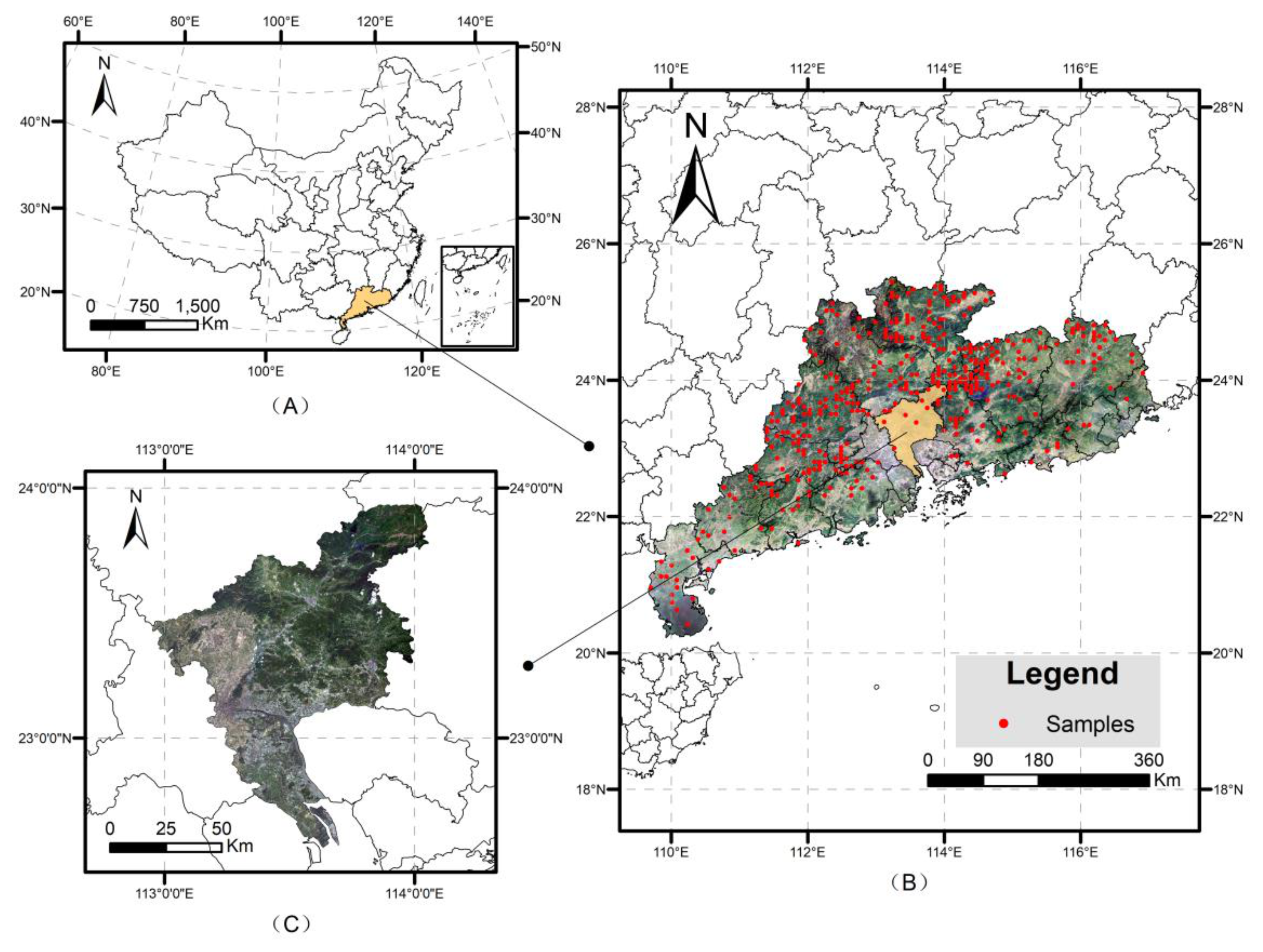
2.1. Study Area

Guangzhou (22°26′–23°56′ N, 112°57′–114°03′ E) is located on the northern edge of the Pearl River Delta in southern China [33] (Figure 1). Stretching across the Tropic of Cancer, Guangzhou has a subtropical, marine monsoon climate with an annual average temperature of 21.4–21.9 °C. The annual precipitation is 1.612–1.909 mm concentrated between April and September [34]. The typical vegetation is subtropical mountain evergreen broad-leaved forest in the north, subtropical evergreen seasonal rainforest in the middle, and tropical evergreen seasonal rainforest in the south.

2.2. Landsat and Field Plots Data

To leverage a large number of Landsat satellite images for research during the period of 1995 to 2015, we used the GEE (Google Earth Engine) platform to process TM and ETM+ data to meet the geometric and radiation quality requirements. GEE users can access and perform the Landsat satellite database in real time and use the Google cloud computing infrastructure to store the results.
Landsat Level-1T (L1T) TOA reflectance data for the six reflective bands of TM and ETM+, along with the collection timestamp, were extracted from the Landsat Archive for the study area and timeframe. A total of 1774 images were used in the study, with stack imageries of 855 Landsat-5 and 919 Landsat-7. The spatial resolution of remote sensing images is 30 m × 30 m, and the cloud cover is below 10%. Nevertheless, these data have been atmospherically corrected using Landsat Disturbance Adaptive Processing System (LEDAPS) correction [35], and include a cloud, shadow, water, and snow mask produced using the C Function of the Mask algorithm (CFMask) [36,37,38], as well as a per-pixel saturation mask.
The sixth consecutive survey of forest resources in Guangdong Province was conducted 14 years ago. The continual inventory system of forest resources in Guangdong was established in 1978. A 25.82 m × 25.82 m plot was established with the intersections of each grid (6 km × 8 km) as reference points. In total, 3685 plots were established in Guangdong. The forest inventory data used in this study contained forest area, geographic locations of plots, stand type, names of dominant species, and forest age.
Finally, a total of 415 sample plots were selected on the basis of forest type, area, age class, and spatial distribution from the inventory in 2007 for carbon density estimation in Guangzhou. Each plot had hundreds of trees with which to examine the tree height and DBH at the height of 1.3 m; approximately 40 thousand trees were calculated in the study. The forest age groups included young, middle-aged, near-mature, mature, and over-mature forests (see Figure 1). The carbon density of each stand could be estimated using the allometric growth function fitting the regression relationship between the biomass and the diameter of the stems, branches, and roots of logged trees in the Pearl River [39]. The regression relationship—using tree height and diameter at breast height of 1.3 m as main predictors—was able to estimate the total biomass of stem, branch, and roots [39]. Meanwhile, we selected the forest field plots collected at Dinghu National Natural Forest Reserve in Zhaoqing city from 2008 to 2014 as the temporal validation samples.

2.3. Subtropical Forest Activities

With the development of urbanization, four kinds of forest activity mainly occurred in Guangdong, including stable forests in the protected area, deforestation, reforestation, and forest management. Given the transition into agriculture (or other), the case was regarded as deforested land. Additionally, the definition of reforestation includes areas regenerated naturally or with the aid of silvicultural measures. Forest management mainly focused on logging-plantation shifts, which return to forest regeneration, except for the long-term natural transition from primary forest to plantation trees. As a result, the logging-plantation shifting consists of carbon emissions and uptake. This means that the carbon sources and pools in the shifting process need to be estimated separately. In total, deforestation and logging activity, as well as slash decomposition, can be regarded as the carbon emission flux. The regrowth and re-planting of forests are both determined carbon pools. Finally, the stable forest growth since 1995 still needs to be accounted for in the increasing carbon uptake, especially with the rapidly increasing density of the middle-aged, near-mature forest.

3. Methods

Remote sensing and geographic information systems (GISs) have been applied to provide land-use change information [40] to determine the different carbon emission factors for forest communities. Time series imagery can be used to simulate the per-pixel function of the emission process and continued factors [41,42]. Nevertheless, high spatial resolution can detect fine-scale LULC changes, even degradation, fire, and withdrawal [42]. Moreover, coarser-resolution pixels could generate more spectral mixtures and spectral heterogeneities of possible forest cover and bare land. Model building was carried out in three steps: (i) Landsat time-series image processing—the GEE platform was used to process the TM and ETM+ data, which meets geometric and radiometric quality requirements. (ii) Change detection by the CCDC algorithm [26] and forest activity were identified according to the transition of biennial land cover and land-use classes. (iii) The dynamics of emission factors were linked with the forest activity process to promote fine-scale bookkeeping model development.

3.1. Fine-Scale Carbon Bookkeeping Model

The bookkeeping model [12] is an empirical IPCC gain-loss model for carbon flux estimation. Two types of information are needed: the conversion rates of each ecosystem and changes per hectare in carbon that follow a change in land use [26]. Allometric growth curves were used to describe how forest changes underwent different disturbances [12]. For example, the assumptions on the response curves for reforestation were delineated as the three stages (fast growth of young and middle-aged forest, slow growth of mature forest, and relative few growths of over-mature forest) for biomass growth and carbon uptake. In deforestation, the aboveground biomass decreased directly, and the timber was discharged according to the wood products. The three products accounted for were fuel woods in a year, paper and book in 10 years, and building and furniture products over approximately 100 years. Moreover, the slash was correlated with the primary carbon density and emitted with the various decay functions. Hence, accurate forest densities and growth curves are crucial in developing a spatially explicit carbon bookkeeping model fitting.

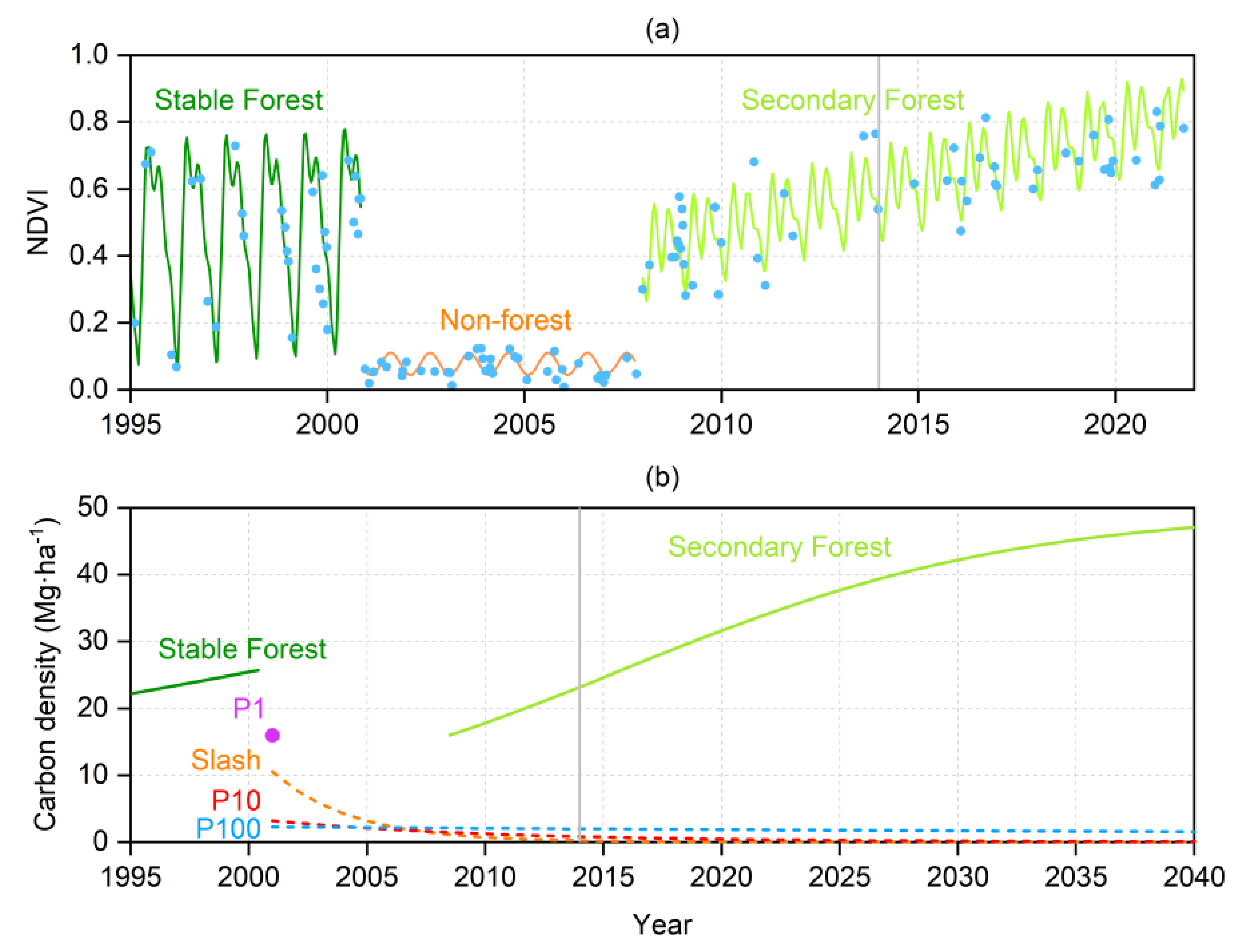
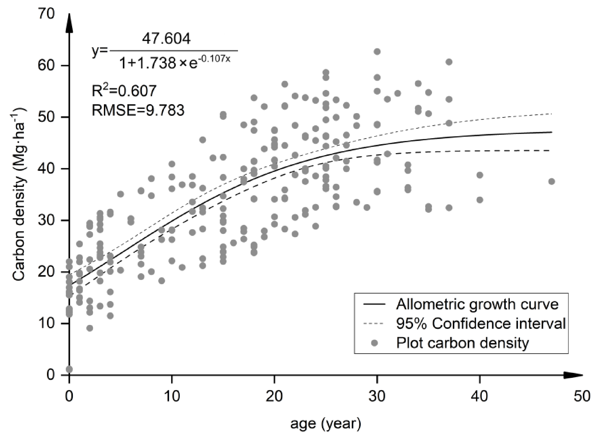
3.1.1. Estimation of Carbon Density

To obtain accurate carbon density estimations in spatial coverage, linear regression and random forest regression were examined and compared in performance of accuracy and correlation. Additionally, the possibility of establishing a temporally explicit growth curve was explored according to the carbon density accumulation of the plots. Hereinafter, 70 percent of samples were used to train the models for linear regression, random forest regression, and growth curve fitting. The remaining 30 percent of samples were used to evaluate the accuracy. The plots in 2014 collected in Dinghu mountain were used to examine the model trained in 2007. To study the continuity of time and space, the spectral index was extracted from Landsat satellite images, and the optimal variables were selected as spatial features, including NDVI, RVI, and the greenness of the tasseled cap transform (TCG) component. In addition, the harmonic coefficients of the harmonic regression model using Landsat time series (LTS) images and terrain variance were taken as the explanatory variables. LTS can delineate the growing trend and seasonal dynamics using harmonic regression parameters (Equation (1)), referred to as LTS-derived metrics. The DEM delineates the forest community related to the terrain elevation and had effects on the spectral response. Therefore, a total of 9 vegetation indices, listed in Table 1 and 18 harmonic coefficients derived from Equation (1) were used to train the regression models.
T S ( i , x ) = a 0 , i + a 1 , i cos ( 2 π T x ) + b 1 , i sin ( 2 π T x ) + c 1 , i x
where T is the number of days per year (T = 365); x is date; i is the ith Landsat band of the following variables; a0,i is the coefficient for overall value; a1,i and b1,i are coefficients for intra-annual change; c1,i is the coefficient for interannual change; TS(i,x) is the fitted reflectance value for the ith Landsat band at date x used to calculate the variables NDVI, RVI, and the TCG component. A total of 18 LTS coefficients were derived from Equation (1) for NDVI, RVI, and the greenness of the TCG. Each index can fit with six coefficients, including the overall value a0,i, the intra-annual change a1,i and b1,i in a year, and a2,i and b2,i in a half year, and the interannual change c1,i.
Additionally, stepwise regression was used to reduce the influence of collinearity problems. The significance level F test was used to examine the significant correlation of variables in the equation. The regression results and accuracy were evaluated using Equation (2):
C d e n = a * N D V I + b * R V I + c * G + d * D E M + ε
The parameters of linear regression Equation (2) were determined to be 39.107, 1.995, 4.581, 0.018, and −0.025; the R2 reached 0.67, and RMSE was 8.718 Mg ha−1.
As a supervised and nonparametric statistical learning technology, RF uses multiple decision trees to make decisions and averages the results of these trees [49,50]. It is an algorithm that processes a large amount of data in a relatively short calculation time, requires fewer adjustment parameters, and is robust to overfitting. The RF regression function can be expressed as:
C d e n = f ( N D V I , R V I , G , C o e f s , D E M )
where Coefs represents the 18 LTS-derived coefficients derived from Equation (1).
To determine the direct relationship between forest age and carbon density, this study fitted the logistic curve equation of tree age as Figure 2. The logistic growth curve is an S-shaped curve, and the equation is as follows:
Y ( t ) = M 1 + a e k t
where Y(t) is the density measure of tree growth in terms of forest age t; M is the maximum density value in general conditions; when y = k/2, x = ln(a)/k, which is the inflection point of the curve; the growth rate starts from fast to slow. a and k are parameters related to the growth rate. The growth function allows one to estimate tree parameters from a biological perspective, such as the difference between primary and secondary plantations.

3.1.2. Forest Activity Detection

To record the rapid LULC change in a complex subtropical forest area, CCDC identified the per-pixel change and calculated the area in Guangzhou from 2000 to 2014 [20,26]. The CCDC algorithm fitted a harmonic model to the time series of remote sensing observations. Given that consecutive observations deviate substantially from the model predictions, a break was labeled; the new harmonic model was initiated after the break, and the coefficients of the models were used in a random forest classifier [51]. The RF classification assigned LULC labels to the time series segments before and after the detected change. First, by using all the available Landsat observations and time series analysis, the predicted synthetic images did not have clouds, cloud shadows, snow, or Landsat 7 SLC-off scan gaps. Second, as the time series models were capable of modeling the seasonality of the data, they avoided some of the problems caused for compositing approaches resulting from vegetation phenology or sun angle effects [52]. Furthermore, forest activity was identified according to the specific carbon emission and uptake, as stated in Section 2.3.

3.1.3. Tracking Carbon Emissions and Uptake

Because large-scale reforestation programs have run since the 1990s’ in Guangdong, we broadened the tracking to obtain LULC change during two periods of 1990–1995 and 1995–2000 using the CCDC methodology. The estimates were derived from a stratified random sample of 1243 units that were selected from a spatially explicit disturbance dataset [26]. Forest activities were easily found, including reforestation and deforestation due to urban extension in the past two decades, and managed forestland, of which logging accounted for 5.57 percent of deforestation, and planting accounted for approximately 7.30 percent of reforestation. In addition, most of the reforestation in the study period has maintained stable growth and fast carbon accumulation for the middle-aged and near-mature forests, of which the carbon fraction needs to be accounted for. Furthermore, the confidence intervals of the four forest activity areas provided uncertainty in tracking the carbon flux (see Table 2).
Since aboveground biomass varies spatially, the amount of carbon loss due to a disturbance would vary accordingly. Therefore, we did not use a single emission factor to represent carbon loss due to disturbance. Instead, a forest pixel case that undergoes a change from deforestation to regrowth was regarded as the carbon loss and uptake as well as the accordingly decomposed process of slash and wood production after the disturbance (see Figure 3). The accurate carbon density estimations in 2007 were used to initiate the four decomposed functions with various emission rates of slash and wood production (1-year, 10-year, and 100-year emission processes as Section 3.1 stated). The carbon emission is the sum of the slash and three decomposed wood productions (Equation (5)), of which each took the same decomposed function (Equations (6) and (7)). Previous studies indicated that the subtropical forest had a higher decay rate than that in the temperate forest [53].
C c l e a r , i = P 1 , i + P 10 , i + P 100 , i + S l a s h P o o l i
P e m i s s i o n , i = P x , i * D R p
S l a s h e m i s s i o n , i = S l a s h P o o l i * ( 1 e D R S l a s h )
where i is year, Cclear,i is the total amount of forest removed in that year; P1,i, P10,i and P100,i, respectively, represent the 1-year, 10-year, and 100-year carbon pool formed by the conversion of removed forest; DRP is the decay rate of P1, P10, and P100; P1 is completely discharged in the next year, and the decay rates of P10 and P100 are taken as 0.1 and 0.01, respectively [54]; DRSlash is the decay rate, taken as 0.3 in subtropical forests [54].

3.2. Accuracy Assessment

The application of ”Good practice” strategy can not only provide a scientific validation design, including sample size and strata location distribution, but also ensure bias-adjusted area estimation. Additionally, cross-validation of R2 and RMSE are accuracy metrics that can be used for carbon density assessments. Both approaches provided accuracy, as expected, but also yielded identical confidence intervals and error ranges for process validation. The spatial patterns before and after disturbance can be mapped for visualization. Hence, the validation results can be presented either in a spatially explicit visualization, such as maps of carbon density, net flux using emissions minus uptake, or in temporal confidence interval statistics (e.g., annual or cumulative).
R 2 = i = 1 n ( y i y ^ i ) 2 i = 1 n ( y i y ¯ ) 2
R M S E = 1 n i = 1 n ( y i y ^ i ) 2
where n is the test sample size; yi is the value of the ith test sample; y ¯ i is the estimated value corresponding to the ith sample point; and y ¯ is the mean value of the test samples.

4. Results

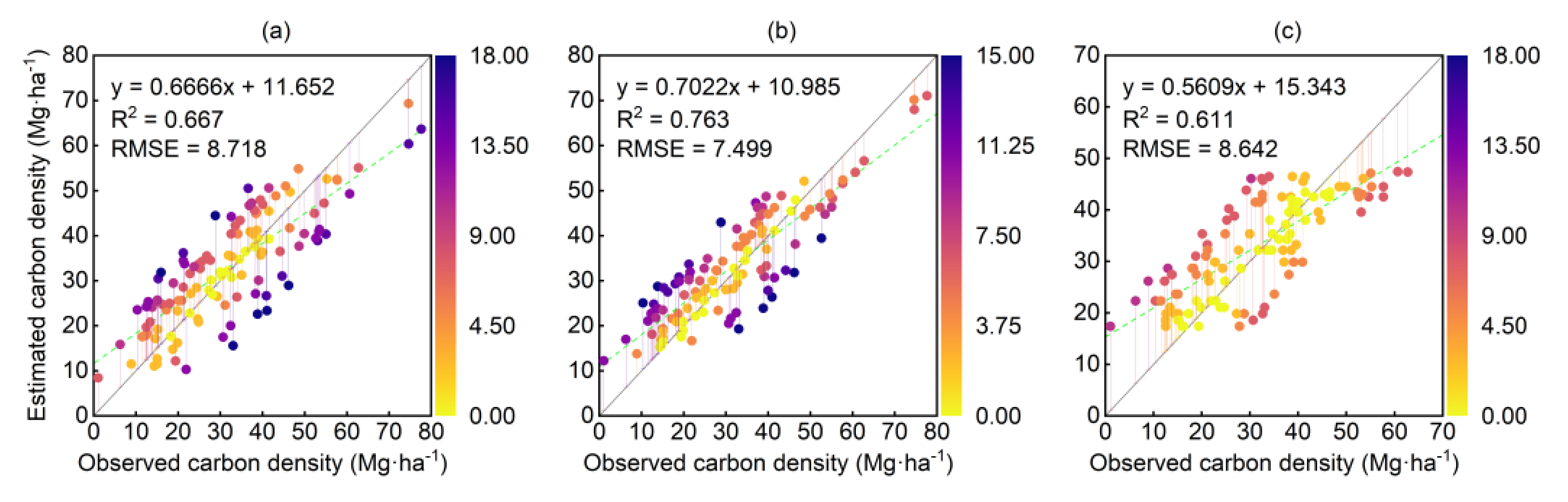
4.1. Carbon Density Estimations

To compare performance, the carbon density estimations using the linear regression Equation (2), random forest, and allometric growth curves were generated and listed as the R2 and RMSE based on the same validation sets (see Figure 4). In spatial detail, random forest had a higher R2 of 0.763 and a smaller RMSE of 7.499 Mg ha−1 than the linear regression, which improved by 0.10 and 1.22 Mg ha−1, respectively. The results suggested that the prediction explains more than 75% of the variance. As the temporal prediction validation, R2 and RMSE were 0.620 and 7.412 Mg ha−1 and were obtained using 215 field plots in Dinghu National subtropical forest reserve. Nevertheless, linear regression also successfully fit the relationship between carbon density and VIs with R2 and RMSE values of 0.67 and 8.78 Mg ha−1 in the study area. The regression function could be adapted for other years without field plots. As for the cloudy images, growth curve fitting was one possible method for carbon estimation constrained by the growth characteristics. By comparison, the random forest served as the estimated method of carbon density in 2007, and the linear regression method can be used for estimation in other years. Importantly, the value in 2007 was regarded as the benchmark of other years.
Meanwhile, it is noted that overestimated low values and underestimated high values existed for the two methods, linear regression and random forest, but the allometric growth curve can mitigate the bias. Too high and low estimations beyond the sum of mean plus/minus two times standard deviation mainly focused on the young forest and over-mature forest. Another is the abnormal value which was smaller than that of the last year and larger than that of the next year. These two outliers needed to be replaced with values estimated by the growth curve using the adjacent two years. As Table 3 shows, there was a highly consistent fitting of density with the field plots, according to the statistics of five forest stages. This demonstrates the reliable density estimation using a combination of random forest and linear regression methods with allometric growth curves.

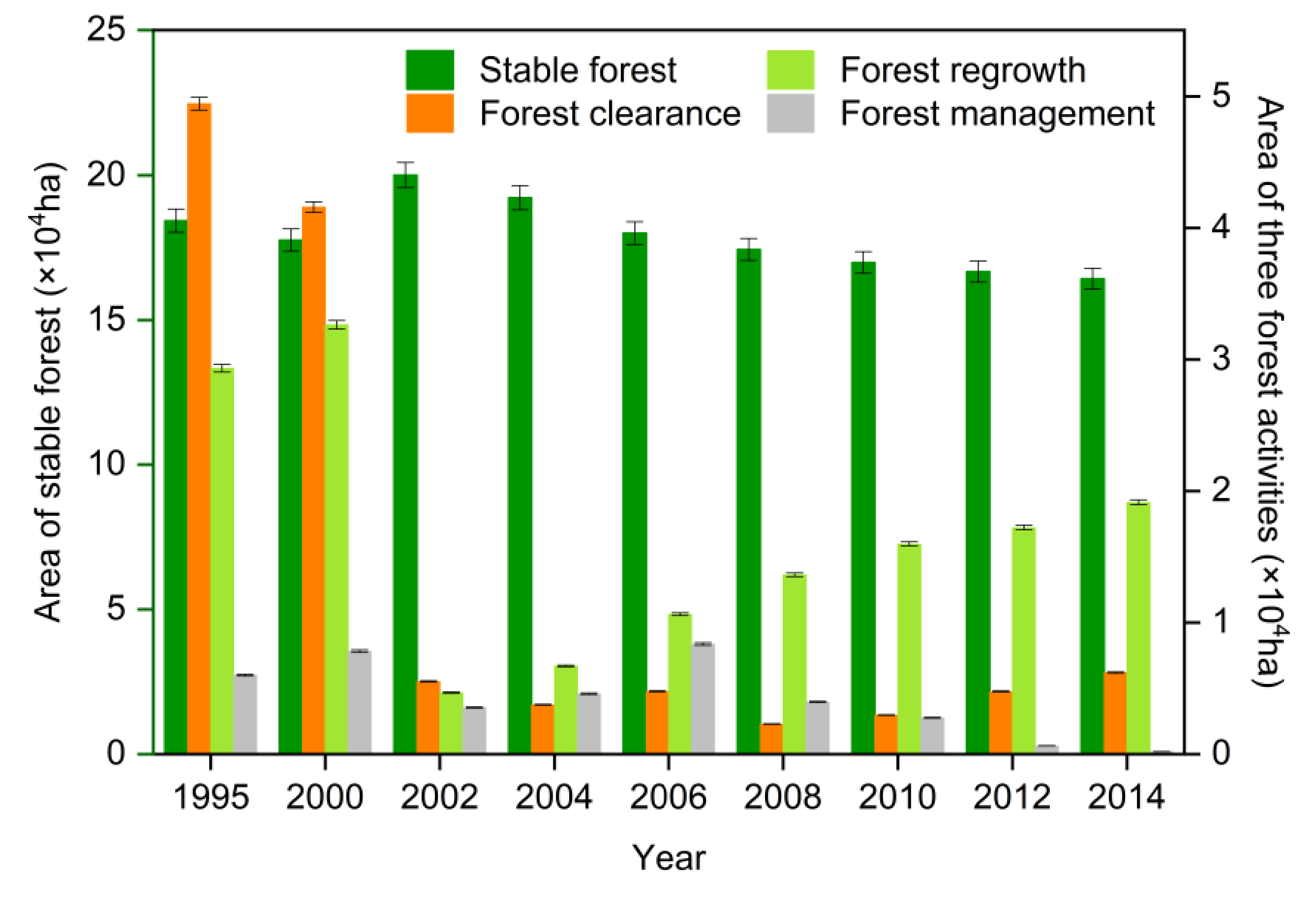
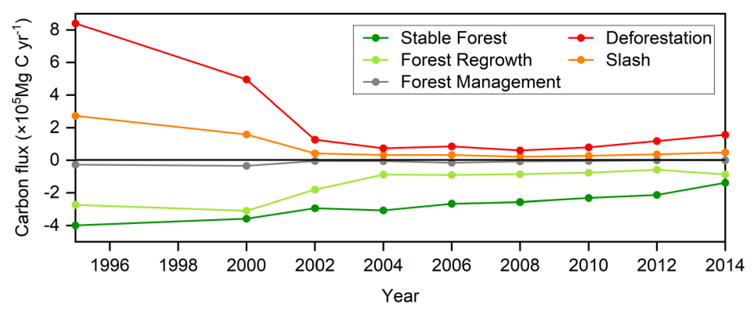
4.2. Biennial Areas and Flux of Forest Activities

According to the accuracy validation of “Good Practice”, the confidence intervals (CI) were calculated as 1.96 multiplied by the standard error of the adjusted change area [22]. This area can provide uncertainty of the area bias for carbon flux estimation (see Figure 5). Hence, the adjusted area with the confidence of different forest activities varied. According to Table 2, deforestation, reforestation, and management activities had high confidence in biennial area estimation, and in this case, the stable forest had relatively low confidence of approximately 1.09%. In Figure 6, forest clearance and regrowth were the dominant activities before 2000, and fine management for regrowth started in 2000. Correspondingly, as Figure 7 shows, the highest carbon emissions of approximately 8.4 × 10⁵ Mg C yr−1 occurred in 1995, and the highest net carbon uptake of approximately 3.5 × 10⁵ Mg C yr−1 occurred in 2002. The net uptake equals the carbon emission minus the carbon uptake, and the uncertainty was estimated correspondingly.

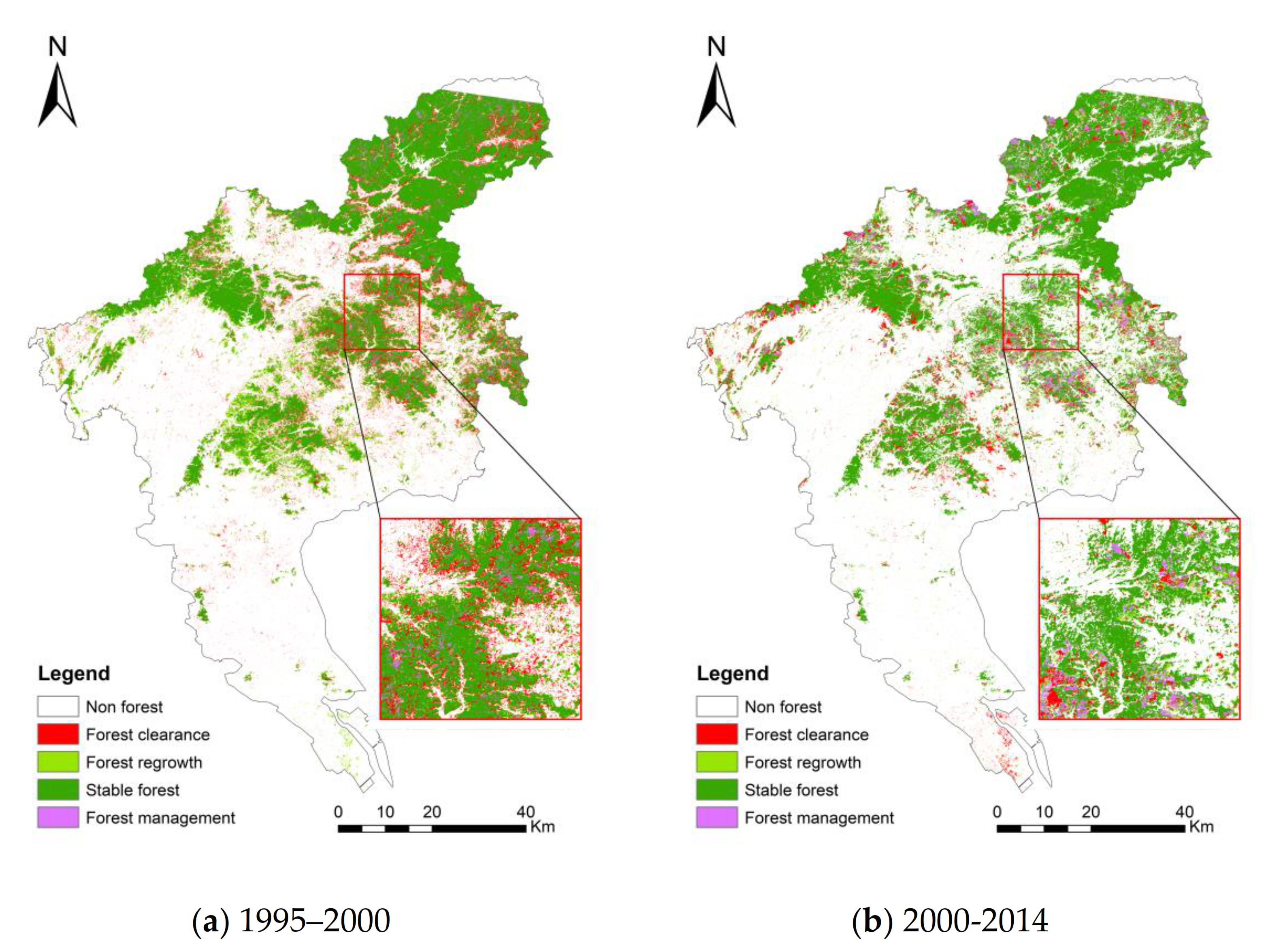
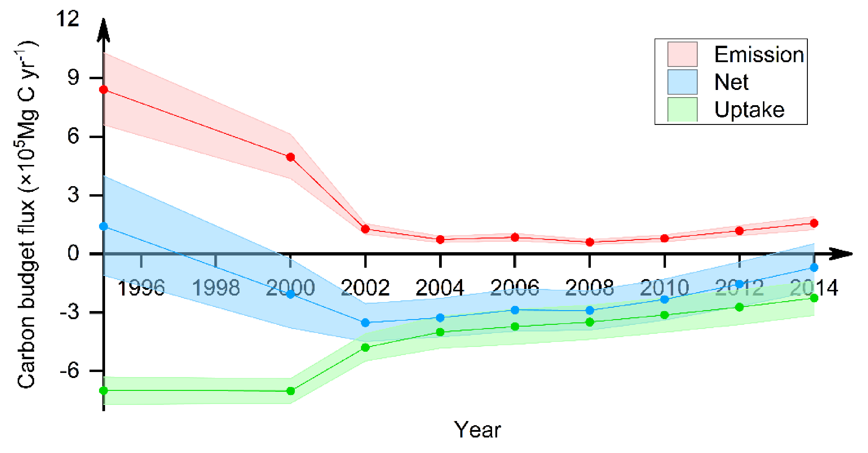
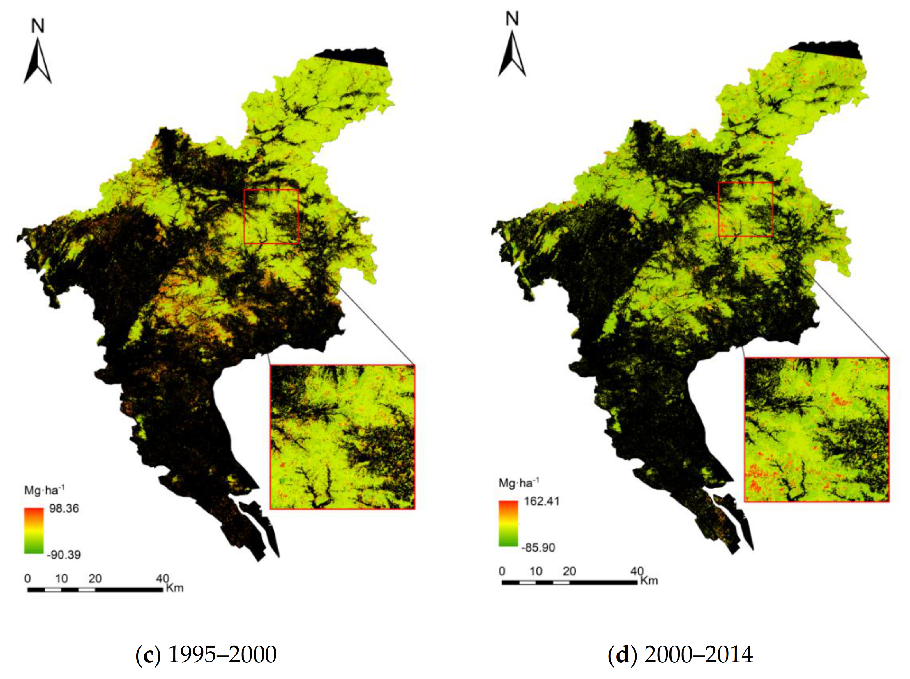
4.3. Spatiotemporal Pattern of Carbon Flux

Time series analysis is capable of checking pixel status in a single year or tracking the total changes pre- and post-urbanization at any given time. Figure 5 shows the change maps generated for Guangzhou between 1995 and 2014. A remarkably large proportion of the study area has changed (34%), and most (71%) have changed only once [22]. As Figure 4 indicates, the tipping point occurred near 2000 from carbon release to uptake, four forest activities, and the corresponding flux statistics of uptake and emission were spatially explicitly mapped before and after 2000. Specifically, Figure 8a,b shows the land cover maps in Guangzhou during the periods of 1995–2000 and 2000–2014. Obvious forest clearance occurred before 1995, and the urban areas have expanded substantially. The shrunk forest area was replaced with cities. Importantly, the reforestation policy was implemented after 1995, and the forest change types were concluded as four kinds in Table 2. As in Figure 5, the forest loss percentage was decreased, and the forest gain fraction increased. Correspondingly, the high-emission pixel locations were consistent with the area of forest clearance that was delineated by the proposed fine-scale carbon accounting methods and forest activity. In contrast, high carbon uptake was located in the northern mountain areas (see in Figure 1).

5. Discussion

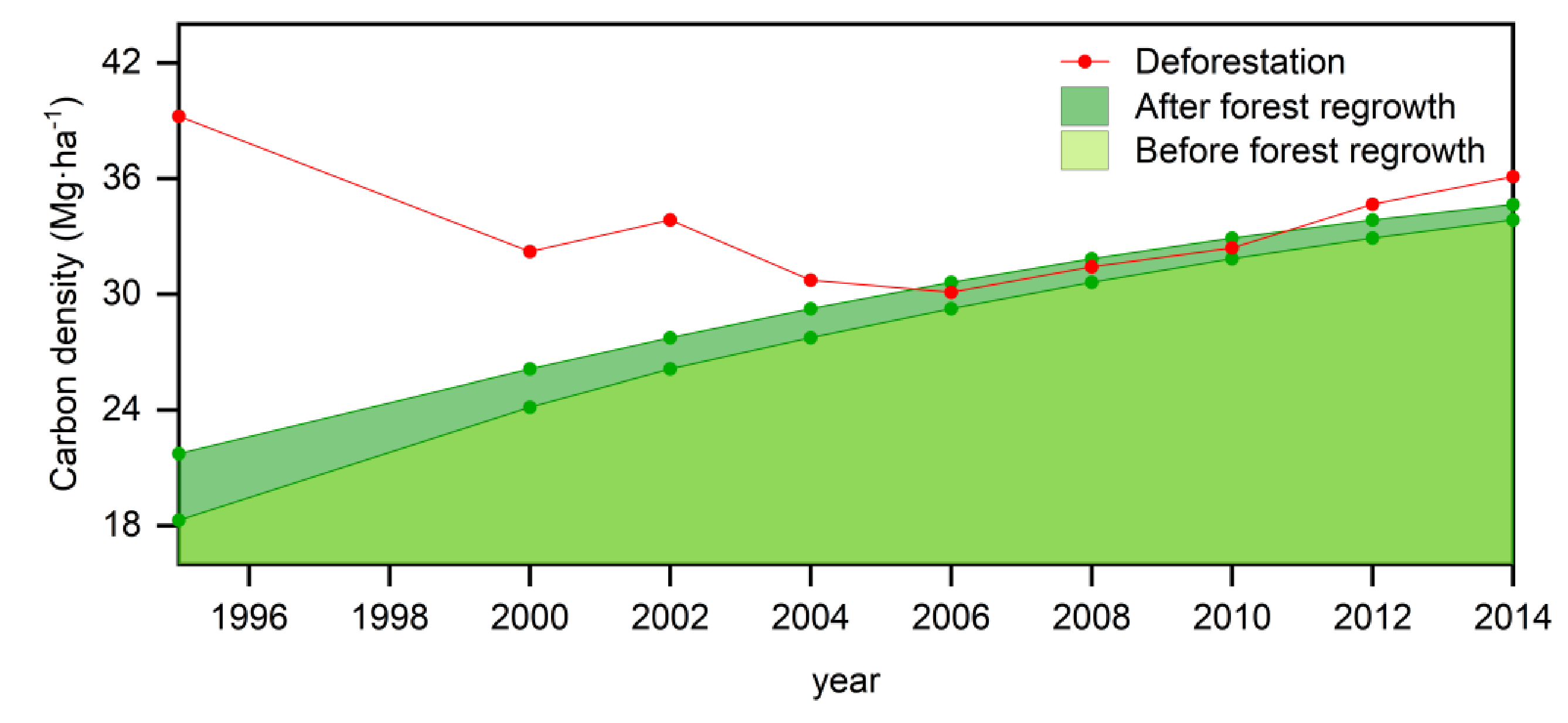
5.1. Trends of Carbon Density Series

The spatial accounting of carbon flux was supported to estimate the density and emission factors according to the forest activity of each pixel. Compared with the original model, using a single factor for the whole forest or forest patch, Figure 9 shows that the mean carbon density value of reforestation improved more than that of before forest regrowth, approximately 5%, 1.55 Mg ha−1. This growth is consistent with the forest survey in the previous study [18]. In addition, we noticed that the carbon density of deforested land showed far higher values than that of the regrowth forest. This demonstrated that regrown forests could positively increase carbon density, but the deforested land would have serious carbon emission capability [19]. As Figure 6 shows, the net carbon flux presents a positive carbon pool, but the carbon emission would be rapidly increased after 2010. The trends of decreased carbon uptake flux should be paid attention to in forest management.

5.2. Comparison with Other Studies

This study proposed a reliable estimation of temporal continuous carbon density using random forest regression to generate data in 2007, based on which the linear regression could generate data for other years. Regarding per-pixel carbon density as a benchmark, the growth curve function was fitted by using the plots of five stand ages and was capable of adjusting the outliers in the adjacent years. The results indicated a temporal continuous prediction capability. This was different from Tang et al., whose research presented an original AGB map benchmark and growth curve fitting from a plot were to predict carbon density [3].
Correspondingly, in carbon density prediction, previous studies reported that the RMSE of the tropical forest biomass estimation using random forest ranged between 68 and 87% of the mean observed biomass in Arizona, and between 61 and 69% in Minnesota [55]. The RMSE of high cover forest in Borneo was approximately 62.8 Mg ha−1, with a mean value of 173.3 Mg ha−1 [55]. Wu et al. suggested that the RF algorithm outperformed R2 (0.63) and RMSE (26.44 Mg ha−1) more than stochastic gradient boosting when using Landsat-based AGB estimation in northwestern Zhejiang Province [56]. Chi et al. revealed that the R2 of the estimated AGB combined with the RF model of Landsat, GLAS, and DEM was 0.72, and the RMSE was 25.24 Mg ha−1 [57]. Our results showed relatively better accuracy than the above studies. The RMSE of density estimation ranged between 78 and 84% of the mean observed biomass in the study area (see in Table 3). Moreover, the carbon density in 2003 in this study was consistent with the field survey of 22.60 Mg ha−1 [5]. Additionally, unlike 1 km MODIS data, 30 m Landsat pixels can provide accurate forest activity area estimations, fine-scale emission function fitting, and emission factors, especially in the logging-regrowth forest management process. Another merit for using Landsat pixels is the same size (25.82 m) as the plots and the advantage of constructing a good relationship between forest activity and the spatial-temporal response of the Landsat images.
Hence, the study not only provided the bias of estimation in random forest, but also proposed to use the allometric growth curve to optimize bias of the too low and too high density estimation by taking the growth characteristics into consideration. By comparison, previous research used the Monte Carlo method to simulate carbon density scope [42]; this study obviously advances the prediction with ground forest growth. Correspondingly, CCDC is capable of tracking land cover change per pixel and providing time-series parameters to drive the bookkeeping model. These methods can be used in others regions or with other data, such as sentinel imagery, given that time series can determine change detection at different scales. For example, in degradation or recovery, in homogeneous spatial or temporal segments, prediction of carbon density and identification of the emission factors could be reliable.

5.3. Limitations

In general, the spatial-temporal tracking method proposed here can mitigate the carbon flux bias by taking the spatial heterogeneity of subtropical forests into consideration. Meanwhile, it also allows us to analyze the forest disturbance effects on carbon. Some questions still need to be improved. (1) Monitoring forest age and structure is important to improve the understanding of the fractions transferred into different carbon pools. (2) Accounting for the degradation effects in the future that are equally as important as the growth of the stable forest in this study. The utilization of SAR, Lidar data would be helpful to simulate or identify the fine-scale bio-parameters of the carbon process. In the future, with the development of remote sensing technology, the model assimilated with more imagery series or ground observation stations, high-resolution series, and multisource imagery could be leveraged to approach the IPCC reporting criteria of unbiasedness.

6. Conclusions

This research implements a spatially explicit bookkeeping model on the Landsat pixel scale. The forest survey data in 2007 in Guangdong Province was used to train and validate the carbon density regression model in spatial coverage as well as to fit the growth curve in temporal coverage. Comprehensive carbon emissions can be identified according to the forest activity transfer process. Therefore, the change detection of deforestation, reforestation, and management in biennial intervals, as well as the growth of stable forest, can be concluded from the consecutive change detection in the case study of Guangzhou. Based on the overall accuracy of 87.5% ± 1.7% for LULC change products, the total forest loss areas were estimated to be 70,206.03 ± 344.01 ha, and other lands transferred to forests were estimated to be approximately 53,556.48 ± 267.78 ha over 1995–2014.
In detail, linear regression, random forest regression, and allometric growth fitting were proposed to obtain reliable per-pixel carbon density estimations by using forest field sampling plots. The results demonstrate that the proposed method is consistent with IPCC tier aims, and outperformed those of previous studies. Moreover, the growth rate from the allometric growth fitting is consistent with the investigation. From 1995 to 2014, the model estimated that a total of (1.02 ± 0.04) × 105 Mg C yr−1 was emitted, while (1.91 ± 0.73) × 105 Mg C yr−1 was sequestered; the net exchange was (0.89 ± 7.67) × 105 Mg C yr−1. This result suggested that the carbon flux of subtropical forests in the study area had a positive carbon uptake pool. Reforestation is an important carbon sequence process, especially the general carbon accumulation from young to near-matured stable forests, which is ignored by traditional research. In general, the spatiotemporal model realizes carbon density and flux dynamics tracking, including the abrupt and gradual change based on fine-scale forest activity. It can provide more comprehensive and detailed feedback on the carbon source and sink change process of forest activities.

Author Contributions

Conceptualization: X.W., R.L. and Y.F.; methodology: X.W. and R.L.; software: X.W. and R.L.; validation: X.W., R.L. and Y.F.; formal analysis: X.W., R.L. and Y.F.; writing-original draft preparation: X.W.; writing-review & editing: Y.F. and H.D.; visualization: R.L.; supervision: Y.F.; funding acquisition: Y.F. All authors have read and agreed to the published version of the manuscript.

Funding

This research was funded by the National Natural Science Foundation of China (grant no. 42071399).

Institutional Review Board Statement

Not applicable.

Informed Consent Statement

Not applicable.

Data Availability Statement

Data from this research will be available upon request to the authors.

Conflicts of Interest

The authors declare no conflict of interest.

References

  1. Le Quéré, C.; Moriarty, R.; Andrew, R.M.; Canadell, J.G.; Sitch, S.; Korsbakken, J.I.; Friedlingstein, P.; Peters, G.P.; Andres, R.J.; Boden, T.A.; et al. Global carbon budget. Earth Syst. Sci. Data 2015, 7, 349–396. [Google Scholar] [CrossRef] [Green Version]
  2. Metcalf, C.J.E.; Graham, A.L.; Huijben, S.; Barclay, V.C.; Long, G.H.; Grenfell, B.T.; Read, A.F.; Bjørnstad, O.N. Partitioning regulatory mechanisms of within-host malaria dynamics using the effective propagation number. Science 2011, 333, 984–988. [Google Scholar] [CrossRef] [PubMed] [Green Version]
  3. Tang, X.; Hutyra, L.R.; Arévalo, P.; Baccini, A.; Woodcock, C.E.; Olofsson, P. Spatiotemporal tracking of carbon emissions and uptake using time series analysis of landsat data: A spatially explicit carbon bookkeeping model. Sci. Total Environ. 2020, 720, 137409. [Google Scholar] [CrossRef]
  4. Shen, W.; Li, M.; Huang, C.; Tao, X.; Wei, A. Annual forest aboveground biomass changes mapped using ICESat/GLAS measurements, historical inventory data, and time-series optical and radar imagery for Guangdong province, China. Agric. For. Meteorol. 2018, 259, 23–38. [Google Scholar] [CrossRef] [Green Version]
  5. Zhou, C.; Wei, X.; Zhou, G.; Yan, J.; Wang, X.; Wang, C.; Liu, H.; Tang, X.; Zhang, Q. Impacts of a large-scale reforestation program on carbon storage dynamics in guangdong, China. For. Ecol. Manag. 2008, 255, 847–854. [Google Scholar] [CrossRef]
  6. Hasan, M.E.; Zhang, L.; Dewan, A.; Guo, H.; Mahmood, R. Spatiotemporal pattern of forest degradation and loss of ecosystem function associated with rohingya influx: A geospatial approach. Land Degrad. Dev. 2021, 32, 3666–3683. [Google Scholar] [CrossRef]
  7. Song, X.P.; Hansen, M.C.; Stehman, S.V.; Potapov, P.V.; Tyukavina, A.; Vermote, E.F.; Townshend, J.R. Global land change from 1982 to 2016. Nature 2018, 560, 639–643. [Google Scholar] [CrossRef]
  8. Pascual, J.I.; Lorente, N.; Song, Z.; Conrad, H.; Rust, H.P. Selectivity in vibrationally mediated single-molecule chemistry. Nature 2003, 423, 525–528. [Google Scholar] [CrossRef]
  9. Reba, M.; Seto, K.C. A Systematic review and assessment of algorithms to detect, characterize, and monitor urban land change. Remote Sens. Environ. 2020, 242, 111739. [Google Scholar] [CrossRef]
  10. Baccini, A.; Walker, W.; Carvalho, L.; Farina, M.; Sulla-Menashe, D.; Houghton, R.A. Tropical forests are a net carbon source based on aboveground measurements of gain and loss. Science 2017, 358, 230–234. [Google Scholar] [CrossRef] [Green Version]
  11. Hansen, M.C.; Loveland, T.R. A review of large area monitoring of land cover change using landsat data. Remote Sens. Environ. 2012, 122, 66–74. [Google Scholar] [CrossRef]
  12. Houghton, R.A.; Hobbie, J.E.; Melillo, J.M.; Moore, B.; Peterson, B.J.; Shaver, G.R.; Woodwell, G.M. Changes in the carbon content of terrestrial biota and soils between 1860 and 1980: A net release of CO"2 to the atmosphere. Ecol. Monogr. 1983, 53, 235–262. [Google Scholar] [CrossRef]
  13. Le Noë, J.; Matej, S.; Magerl, A.; Bhan, M.; Erb, K.H.; Gingrich, S. Modeling and empirical validation of long-term carbon sequestration in forests (France, 1850–2015). Glob. Chang. Biol. 2020, 26, 2421–2434. [Google Scholar] [CrossRef] [Green Version]
  14. Lienert, S.; Joos, F. A bayesian ensemble data assimilation to constrain model parameters and land-use carbon emissions. Biogeosciences 2018, 15, 2909–2930. [Google Scholar] [CrossRef] [Green Version]
  15. Global Forest Observations Initiative (GFOI). Integration of Remote-Sensing and Ground-Based Observations for Estimation of Emissions and Removals of Greenhouse Gases in Forests: Methods and Guidance from the Global Forest Observations Initiative Integration of Remote-Sensing and Ground-Based Observations for Estimation of Emissions and Removals of Greenhouse Gases in Forests, 2nd ed.; UN Food and Agriculture Organization: Rome, Italy, 2016; pp. 1–224. [Google Scholar]
  16. He, L.; Chen, J.M.; Pan, Y.; Birdsey, R.; Kattge, J. Relationships between net primary productivity and forest stand age in U.S. forests. Global Biogeochem. Cycles 2012, 26, 3009. [Google Scholar] [CrossRef]
  17. Fang, L.; Yang, J.; Zhang, W.; Zhang, W.; Yan, Q. Combining allometry and landsat-derived disturbance history to estimate tree biomass in subtropical planted forests. Remote Sens. Environ. 2019, 235, 111423. [Google Scholar] [CrossRef]
  18. Poorter, L.; Bongers, F.; Aide, T.M.; Almeyda Zambrano, A.M.; Balvanera, P.; Becknell, J.M.; Boukili, V.; Brancalion, P.H.S.; Broadbent, E.N.; Chazdon, R.L.; et al. Biomass resilience of neotropical secondary forests. Nature 2016, 530, 211–214. [Google Scholar] [CrossRef]
  19. Yue, C.; Ciais, P.; Houghton, R.A.; Nassikas, A.A. Contribution of land use to the interannual variability of the land carbon cycle. Nat. Commun. 2020, 11, 3170. [Google Scholar] [CrossRef]
  20. Zhu, Z.; Fu, Y.; Woodcock, C.E.; Olofsson, P.; Vogelmann, J.E.; Holden, C.; Wang, M.; Dai, S.; Yu, Y. Including land cover change in analysis of greenness trends using all available landsat 5, 7, and 8 images: A case study from Guangzhou, China (2000–2014). Remote Sens. Environ. 2016, 185, 243–257. [Google Scholar] [CrossRef] [Green Version]
  21. Fu, Y.; Li, J.; Weng, Q.; Zheng, Q.; Li, L.; Dai, S.; Guo, B. Characterizing the Spatial Pattern of Annual Urban Growth by Using Time Series Landsat Imagery. Sci. Total Environ. 2019, 666, 274–284. [Google Scholar] [CrossRef]
  22. Fu, Y.; Lu, X.; Zhao, Y.; Zeng, X.; Xia, L. Assessment Impacts of Weather and Land Use/Land Cover (LULC) Change on Urban Vegetation Net Primary Productivity (NPP): A Case Study in Guangzhou, China. Remote Sens. 2013, 5, 4125–4144. [Google Scholar] [CrossRef] [Green Version]
  23. Kennedy, R.E.; Cohen, W.B.; Schroeder, T.A. Trajectory-Based Change Detection for Automated Characterization of Forest Disturbance Dynamics. Remote Sens. Environ. 2007, 110, 370–386. [Google Scholar] [CrossRef]
  24. Zhu, Z.; Wulder, M.A.; Roy, D.P.; Woodcock, C.E.; Hansen, M.C.; Radeloff, V.C.; Healey, S.P.; Schaaf, C.; Hostert, P.; Strobl, P. Benefits of the free and open landsat data policy. Remote Sens. Environ. 2019, 224, 382–385. [Google Scholar] [CrossRef]
  25. Wulder, M.A.; Loveland, T.R.; Roy, D.P.; Crawford, C.J.; Masek, J.G.; Woodcock, C.E.; Allen, R.G.; Anderson, M.C.; Belward, A.S.; Cohen, W.B. Current status of landsat program, science, and applications. Remote Sens. Environ. 2019, 225, 127–147. [Google Scholar] [CrossRef]
  26. Zhu, Z.; Woodcock, C.E. Continuous change detection and classification of land cover using all available landsat data. Remote Sens. Environ. 2014, 144, 152–171. [Google Scholar] [CrossRef] [Green Version]
  27. Hansen, M.; Potapov, P.; Margono, B.; Stehman, S.; Turubanova, S.; Tyukavina, A. Response to comment on “high-resolution global maps of 21st-century forest cover change”. Science 2014, 344, 981. [Google Scholar] [CrossRef] [Green Version]
  28. Kumar, R.; Gupta, S.R.; Singh, S.; Patil, P.; Dhadhwal, V.K. Spatial distribution of forest biomass using remote sensing and regression models in Northern Haryana, India. Int. J. Ecol. 2011, 37, 37–47. [Google Scholar]
  29. Li, B.; Wang, W.; Bai, L.; Chen, N.; Wang, W. Estimation of aboveground vegetation biomass based on landsat-8 OLI satellite images in the Guanzhong basin, China. Int. J. Remote Sens. 2019, 40, 3927–3947. [Google Scholar] [CrossRef]
  30. Cao, L.; Coops, N.C.; Hermosilla, T.; Innes, J.; Dai, J.; She, G. Using small-footprint discrete and full-waveform airborne LiDAR metrics to estimate total biomass and biomass components in subtropical forests. Remote Sens. 2014, 6, 7110–7135. [Google Scholar] [CrossRef] [Green Version]
  31. Wang, X.; Shao, G.; Chen, H.; Lewis, B.J.; Qi, G.; Yu, D.; Zhou, L.; Dai, L. An application of remote sensing data in mapping landscape-level forest biomass for monitoring the effectiveness of forest policies in Northeastern China. Environ. Manag. 2013, 52, 612–620. [Google Scholar] [CrossRef]
  32. Sarker, L.R.; Nichol, J.E. Improved forest biomass estimates using ALOS AVNIR-2 texture indices. Remote Sens. Environ. 2011, 115, 968–977. [Google Scholar] [CrossRef]
  33. Guangzhou Yearbook Compilation Committee. Administrative Division and Weather. In Guangzhou Yearbook; Guangzhou Yearbook Press: Guangzhou, China, 2010; Chapter 1; pp. 4–5. (In Chinese) [Google Scholar]
  34. Local Chronicles Compilation Committee of Guangzhou. Natural Geography. In Annals of Guangzhou; Guangzhou Press: Guangzhou, China, 1998; Volume 2, pp. 42–49. (In Chinese) [Google Scholar]
  35. Masek, J.G.; Vermote, E.F.; Saleous, N.E.; Wolfe, R.; Hall, F.G.; Huemmrich, K.F.; Gao, F.; Kutler, J.; Lim, T.K. A landsat surface reflectance dataset for North America, 1990-2000. IEEE Geosci. Remote S 2006, 3, 68–72. [Google Scholar] [CrossRef]
  36. Zhu, Z.; Woodcock, C.E. Object-based cloud and cloud shadow detection in landsat imagery. Remote Sens. Environ. 2012, 118, 83–94. [Google Scholar] [CrossRef]
  37. Zhu, Z.; Wang, S.; Woodcock, C.E. Improvement and expansion of the fmask algorithm: Cloud, cloud shadow, and snow detection for landsats 4-7, 8, and sentinel 2 images. Remote Sens. Environ. 2015, 159, 269–277. [Google Scholar] [CrossRef]
  38. Foga, S.; Scaramuzza, P.L.; Guo, S.; Zhu, Z.; Dilley, R.D.; Beckmann, T.; Schmidt, G.L.; Dwyer, J.L.; Joseph Hughes, M.; Laue, B. Cloud detection algorithm comparison and validation for operational landsat data products. Remote Sens. Environ. 2017, 194, 379–390. [Google Scholar] [CrossRef] [Green Version]
  39. Zhao, H.; Li, Z.; Zhou, G.; Qiu, Z.; Wu, Z. Site-specific allometric models for prediction of above-and belowground biomass of subtropical forests in Guangzhou, Southern China. Forests 2019, 10, 862. [Google Scholar] [CrossRef] [Green Version]
  40. Olofsson, P.; Torchinava, P.; Woodcock, C.E.; Baccini, A.; Houghton, R.A.; Ozdogan, M.; Zhao, F.; Yang, X. Implications of land use change on the national terrestrial carbon budget of Georgia. Carbon Balance Manag. 2010, 5, 1–13. [Google Scholar] [CrossRef] [Green Version]
  41. Tang, X.; Woodcock, C.E.; Olofsson, P.; Hutyra, L.R. Spatiotemporal assessment of land use/land cover change and associated carbon emissions and uptake in the mekong river basin. Remote Sens. Environ. 2021, 256, 112336. [Google Scholar] [CrossRef]
  42. Bullock, E.L.; Woodcock, C.E. Carbon loss and removal due to forest disturbance and regeneration in the amazon. Sci. Total Environ. 2021, 764, 142839. [Google Scholar] [CrossRef] [PubMed]
  43. Tian, J.Q.; Min, X.J. Advances in vegetation index research. Adv. Earth Sci. 1998, 13, 327–333. (In Chinese) [Google Scholar]
  44. Zhang, R.H.; Rao, N.X.; Liao, K.N. Approach for a vegetation index resistant to atmospheric effect. Acta Bot. Sin. 1996, 1, 53–62. [Google Scholar]
  45. Pinty, B.; Verstraete, M.M. GEMI: A Non-Linear Index to Monitor Global Vegetation from Satellites. Vegetatio 1992, 101, 15–20. [Google Scholar] [CrossRef]
  46. Qi, J.; Chehbouni, A.; Huete, A.R.; Kerr, Y.H.; Sorooshian, S. A Modified soil adjusted vegetation index. Remote Sens. Environ. 1994, 48, 119–126. [Google Scholar] [CrossRef]
  47. Kauth, R.J.; Thomas, G.S. The Tasselled Cap—A Graphic Description of the Spectral-Temporal Development of Agricultural Crops as Seen by LANDSAT. LARS Symposia 1976, 159. [Google Scholar]
  48. Tang, G. Progress of DEM and Digital Terrain Analysis in China. Acta Geogr. Sin. 2014, 69, 1305–1325. (In Chinese) [Google Scholar]
  49. He, H.; Garcia, E.A. Learning from Imbalanced Data. IEEE Trans. Knowl. Data Eng. 2009, 21, 1263–1284. [Google Scholar]
  50. Hu, X.; Hartmann Belle, J.; Meng, X.; Wildani, A.; Waller, L.; Strickland, M.; Liu, Y. Estimating PM2.5 concentrations in the conterminous United States using the random forest approach. Environ. Sci. Technol. 2017, 51, 6936–6944. [Google Scholar] [CrossRef]
  51. Breiman, L. Random Forests. Mach. Learn. 2001, 45, 5–32. [Google Scholar] [CrossRef] [Green Version]
  52. Zhu, Z.; Woodcock, C.E.; Holden, C.; Yang, Z. Generating synthetic landsat images based on all available landsat data: Predicting landsat surface reflectance at any given time. Remote Sens. Environ. 2015, 162, 67–83. [Google Scholar] [CrossRef]
  53. Zhang, D.Q.; Ye, W.H.; Yu, Q.F.; Kong, G.H.; Zhang, Y.C. Study on representative forest litter in Dinghushan succession series. J. Ecol. 2000, 6, 938–944. [Google Scholar]
  54. Houghton, R.A.; Hackler, J.L. Emissions of carbon from forestry and land-use change in tropical Asia. Glob. Chang. Biol. 1999, 5, 481–492. [Google Scholar] [CrossRef]
  55. Hayashi, M.; Motohka, T.; Sawada, Y. Aboveground biomass mapping using ALOS-2/PALSAR-2 time-series images for borneo’s forest. IEEE J. Sel. Top. Appl. Earth. Obs. Remote Sens. 2019, 12, 5167–5177. [Google Scholar] [CrossRef]
  56. Wu, C.; Shen, H.; Shen, A.; Deng, J.; Gan, M.; Zhu, J.; Xu, H.; Wang, K. Comparison of machine-learning methods for above-ground biomass estimation based on landsat imagery. J. Appl. Remote Sens. 2016, 10, 035010. [Google Scholar] [CrossRef]
  57. Chi, H.; Sun, G.; Huang, J.; Li, R.; Ren, X.; Ni, W.; Fu, A. Estimation of forest aboveground biomass in Changbai mountain region using ICESat/GLAS and landsat/TM Data. Remote Sens. 2017, 9, 707. [Google Scholar] [CrossRef] [Green Version]
Figure 1. Figure (A) shows the scope of China’s national boundaries and the location of Guangdong Province, figure (B) shows the distribution of sample points in Guangdong Province and the location of Guangzhou, and figure (C) shows the scope of Guangzhou.
Remotesensing 14 00753 g001
Figure 2. Scatterplot diagram of the allometric growth curve fitting.
Remotesensing 14 00753 g002
Figure 3. Panel (a) shows Landsat time series of NDVI and change segments identified by the CCDC model for a pixel. Panel (b) shows the carbon density trends of different carbon pools associated with the land cover dynamics of this pixel. NDVI and carbon density profiles for forest clearance or regrowth in a pixel suggested consistent trends. In particular, the carbon uptake effect of forest regrowth and the carbon emission effect of forest loss are obvious.
Remotesensing 14 00753 g003
Figure 4. Carbon density estimation and validation for linear regression (a), random forest regression (b), and allometric growth curve fitting (c).
Remotesensing 14 00753 g004
Figure 5. Changed area of four forest activities and the area bias estimated by the stratified samples based on “Good Practice” strategy over 1995–2014.
Remotesensing 14 00753 g005
Figure 6. Carbon emission and uptake details of forest activities, suggesting pool capabilities for Guangzhou over 1995–2014.
Remotesensing 14 00753 g006
Figure 7. Carbon flux with 95% confidence intervals for Guangzhou over 1995–2014.
Remotesensing 14 00753 g007
Figure 8. Spatial profile for the four forest activities over 1995–2000 (a), corresponding carbon flux (c), and those over 2000–2014 (b,d) in Guangzhou.
Remotesensing 14 00753 g008aRemotesensing 14 00753 g008b
Figure 9. Biennial carbon density profile of variation of deforestation and reforestation.
Remotesensing 14 00753 g009
Table 1. Description of spectral indices for carbon density estimation.
VariablesEquation or Description
DVI [43] ρ n i r ρ r e d
RVI [43] ρ n i r / ρ r e d
NDVI [44] ρ n i r ρ r e d / ρ n i r + ρ r e d
EVI [45] C * ( ρ n i r ρ r e d ) / ρ n i r + C 1 * ρ r e d C 2 * ρ b l u e + L
MSAVI [46] ( 2 * ρ n i r + 1 ( 2 * ρ n i r + 1 ) 2 8 * ( ρ n i r ρ r e d ) ) / 2
TCG [47]Greenness of tasseled cap transform
TCB [47]Brightness of tasseled cap transform
TCW [47]Wetness of tasseled cap transform
DEM [48]30 m SRTM DEM
Table 2. Stratified estimators of area ± CI% of total map area from 1995 to 2014.
Stable ForestForest ClearanceForest RegrowthForest Management
Area(ha)204,84070,206.0353,556.4833,131.97
95%CI1.09%0.49%0.50%0.64%
Table 3. Comparison of carbon density estimation with the field sample plots using the combination of random forest regression with allometric growth curve fitting.
Young Forest
(0–9)
Middle-Aged Forest
(10–25)
Near-Mature Forest
(26–35)
Mature Forest
(36–42)
Overmature Forest
(>42)
Counts491061476449
PlotsMean20.5930.2733.4133.9934.40
Maximum38.6059.0259.9781.8174.89
Minimum5.0710.1611.3112.3213.26
Standard deviation9.0012.2212.2812.6717.61
EstimationsMean25.5333.6635.1033.6332.42
Maximum43.9253.4258.7057.7767.34
Minimum13.4715.0317.6116.2615.71
Standard deviation6.519.739.8010.4013.19
RMSE ratio21.78%16.47%17.37%18.25%19.02%1
Publisher’s Note: MDPI stays neutral with regard to jurisdictional claims in published maps and institutional affiliations.

