
Land Subsidence Monitoring Method in Regions of Variable Radar Reflection Characteristics by Integrating PS-InSAR and SBAS-InSAR Techniques


Abstract
:1. Introduction
2. Methodology
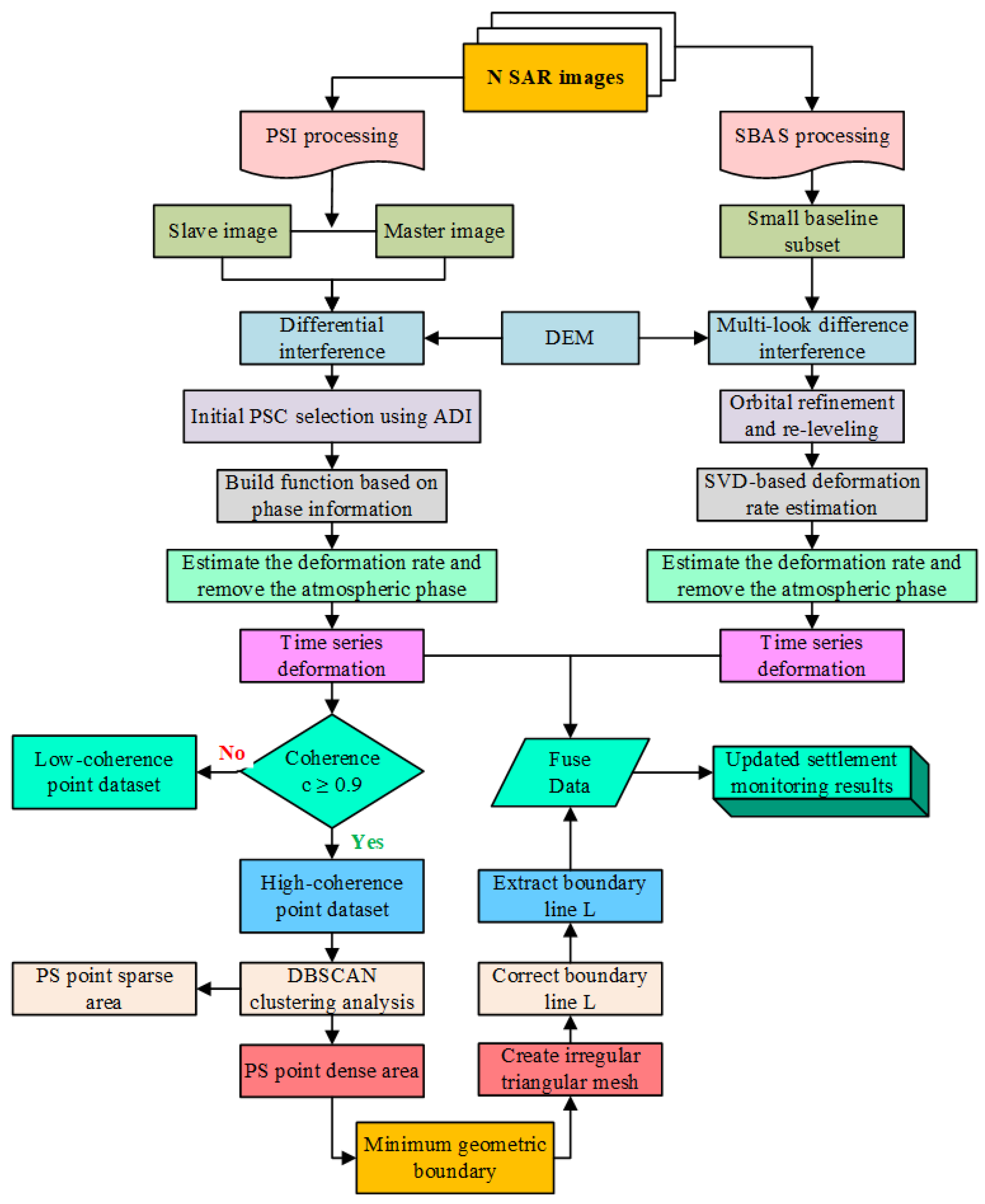
2.1. Proposed Method
2.2. Time Series InSAR Analysis Method
3. Study Area and SAR Datasets
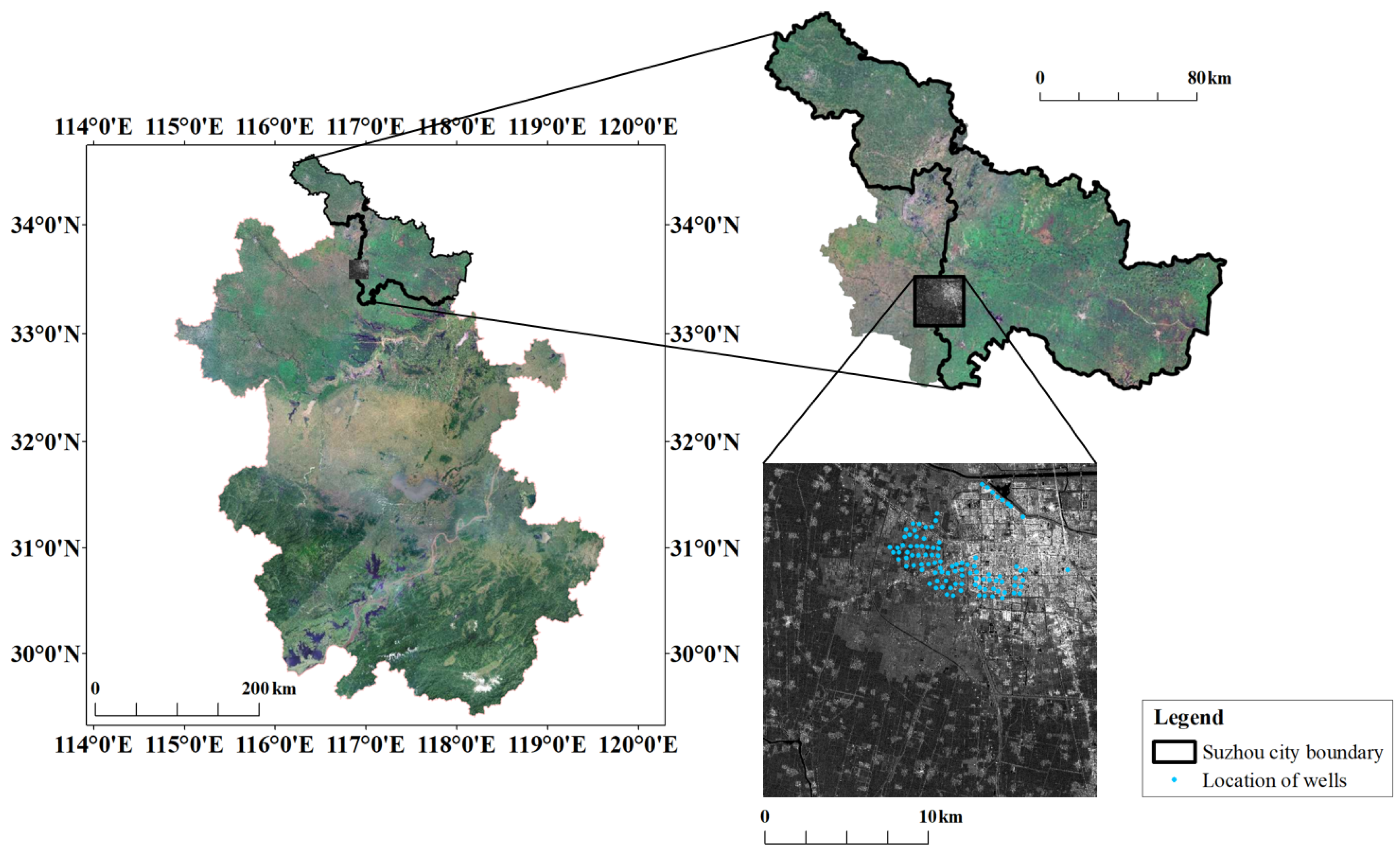
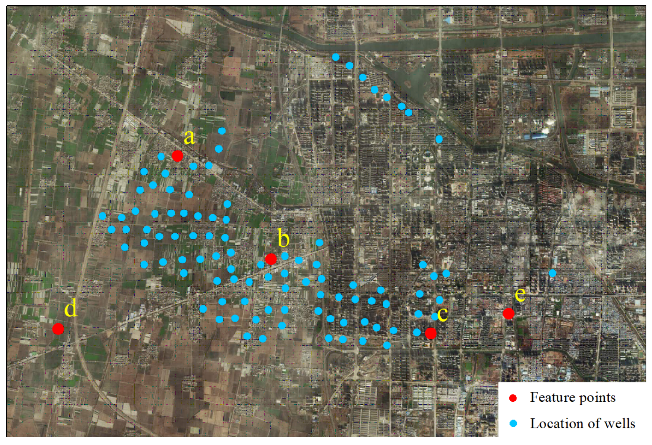
3.1. Study Area
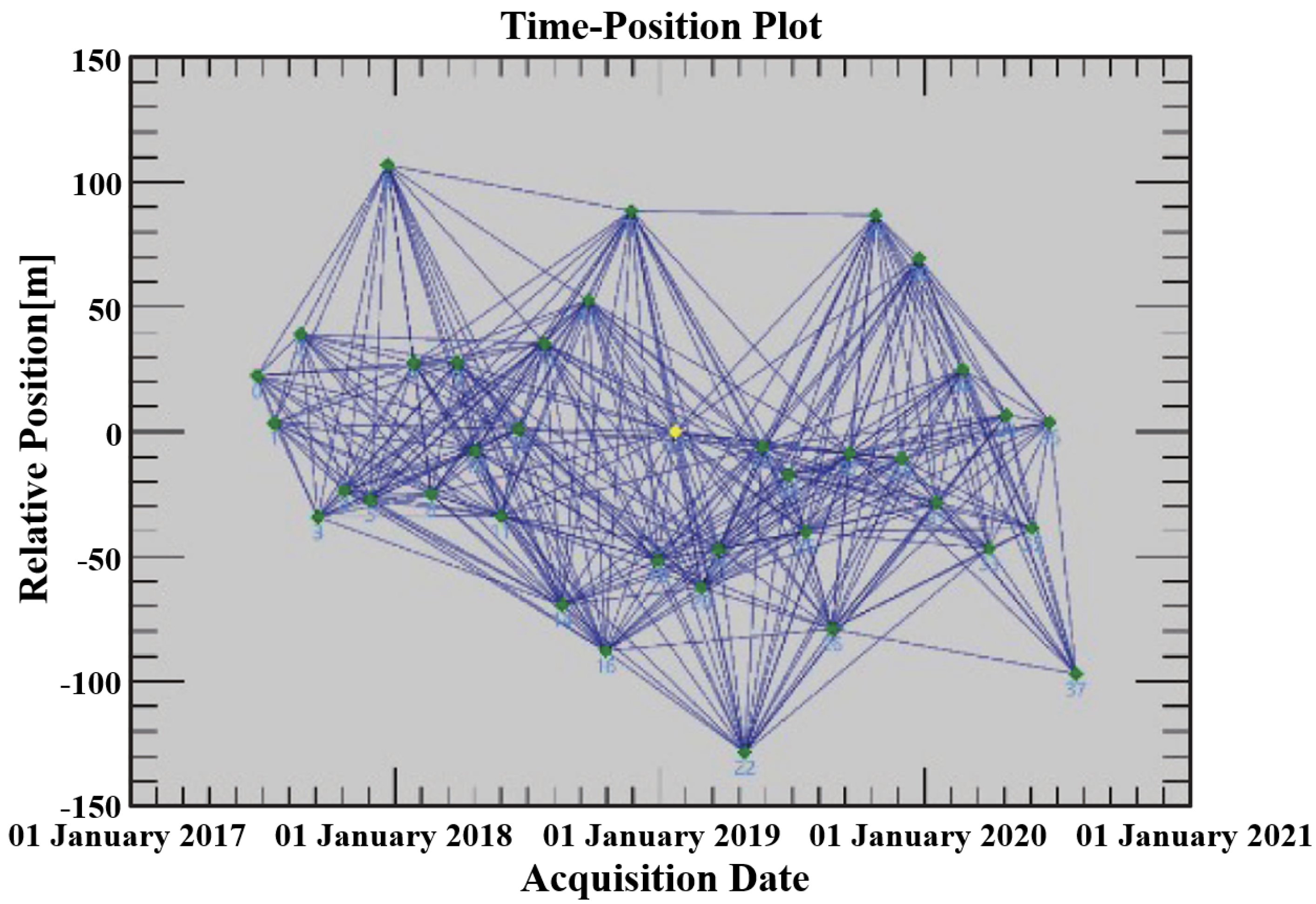
3.2. SAR Datasets
4. Comparison of Single Interferometry
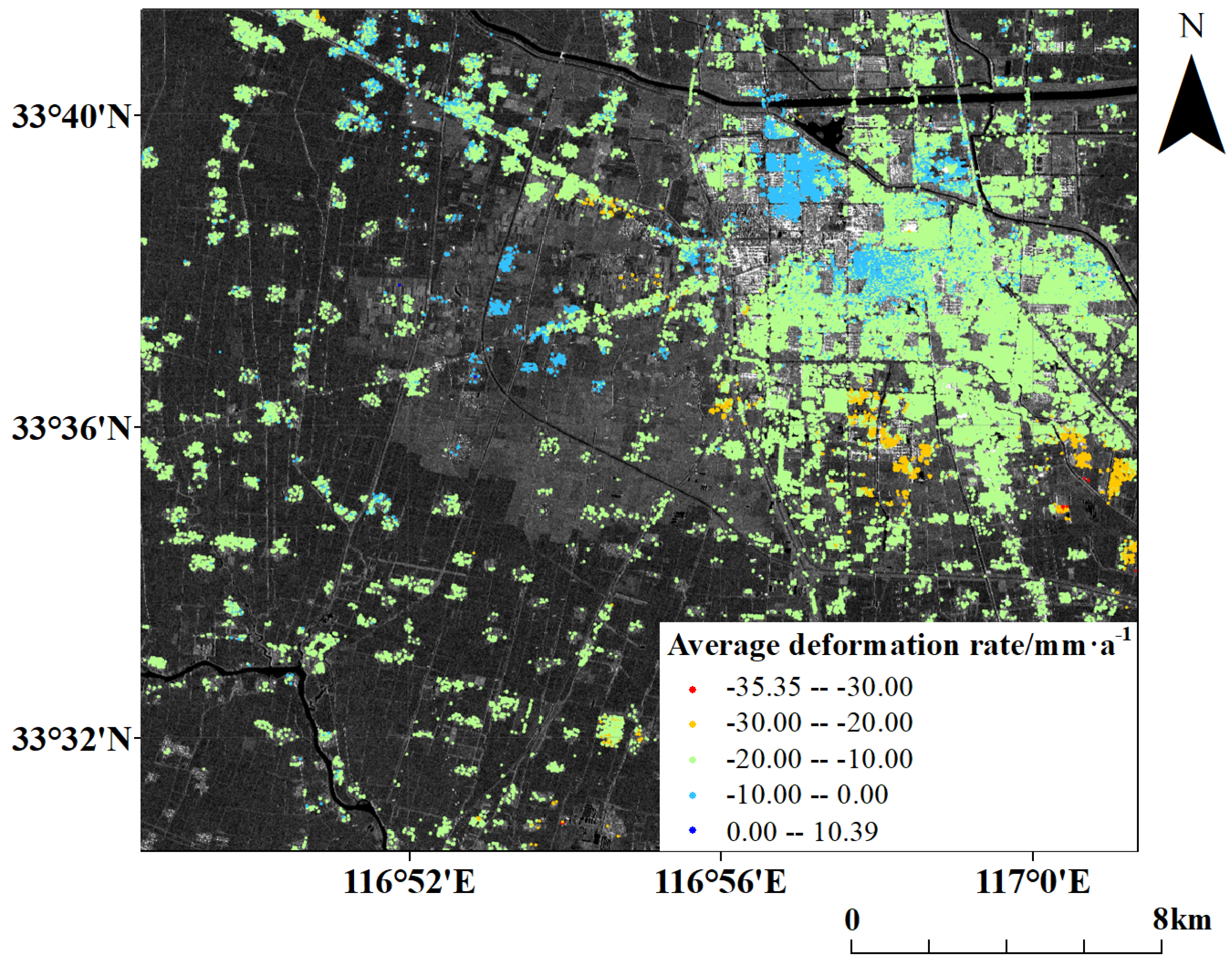
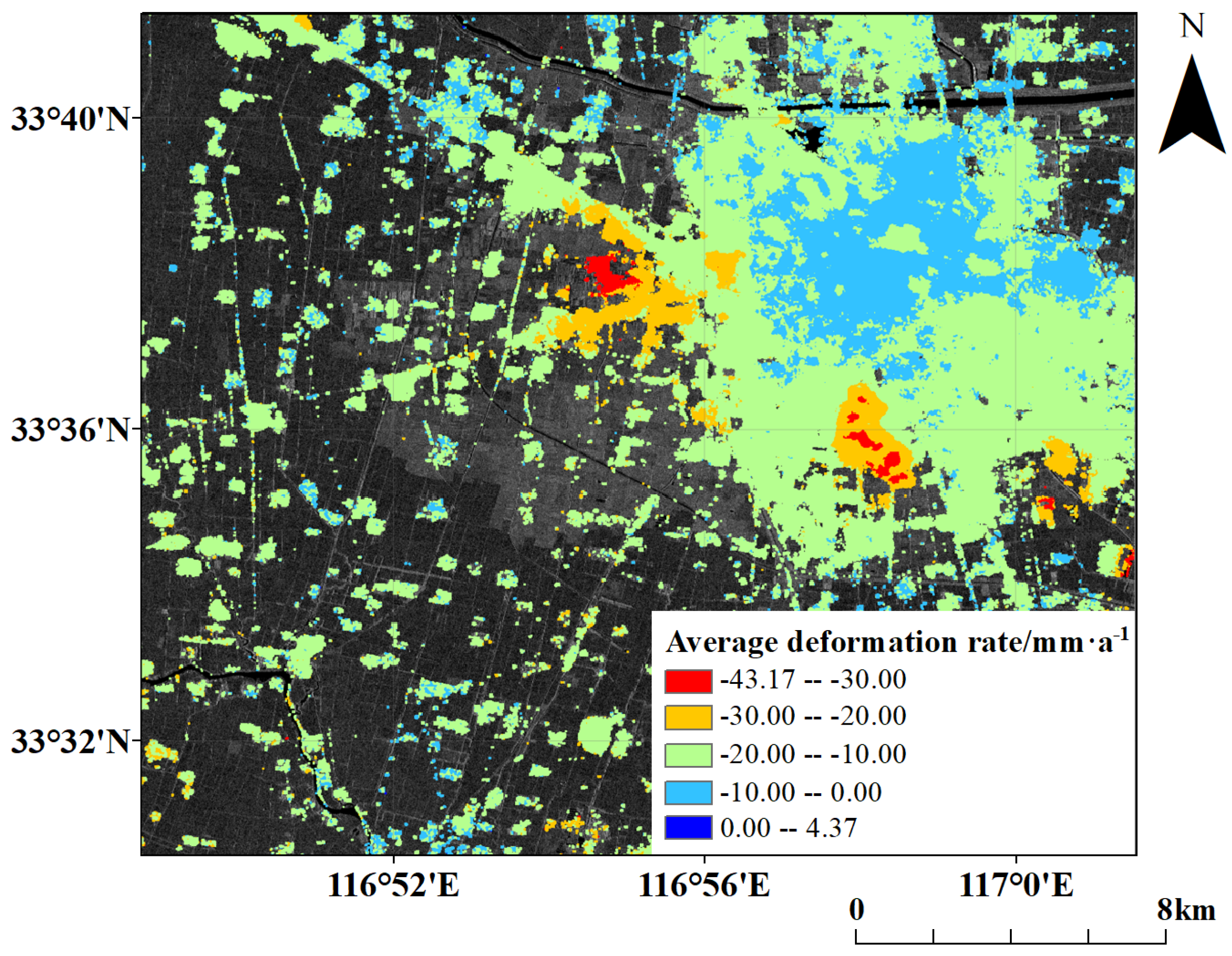
4.1. Result of PS-InSAR Processing
4.2. Result of SBAS-InSAR Processing
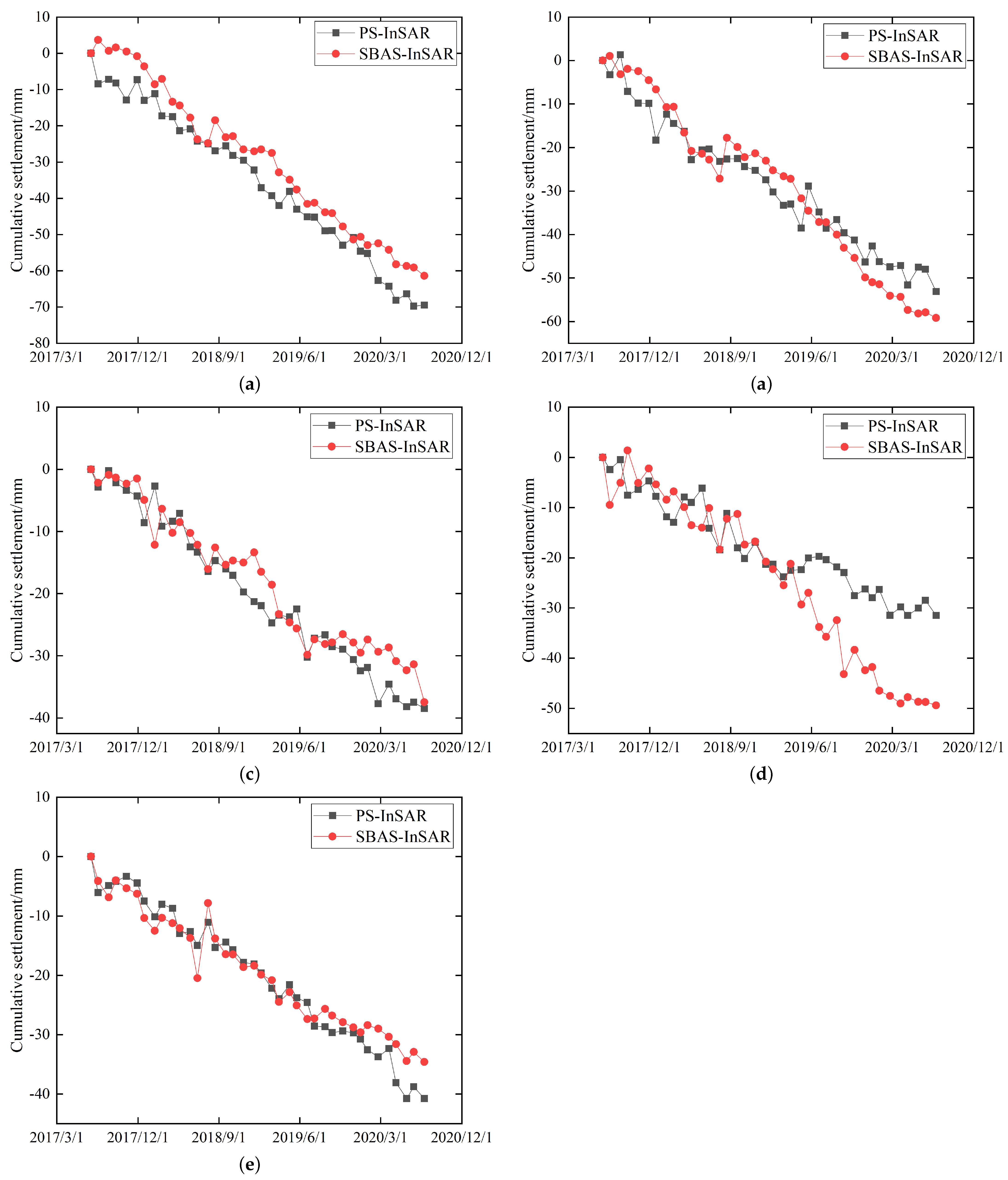
4.3. Results Comparison of PS-InSAR and SBAS-InSAR
5. Fusion of PS-InSAR and SBAS-InSAR
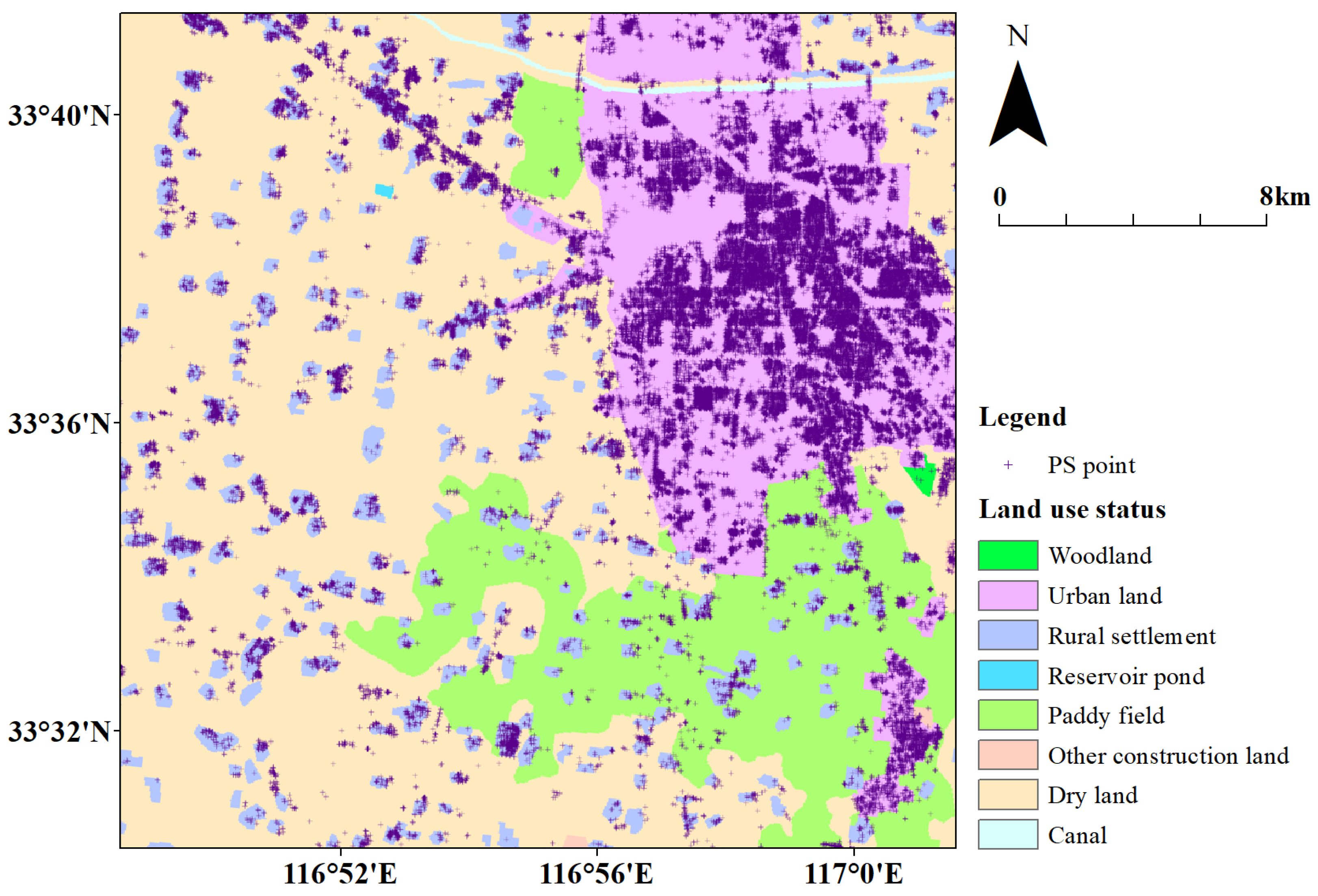
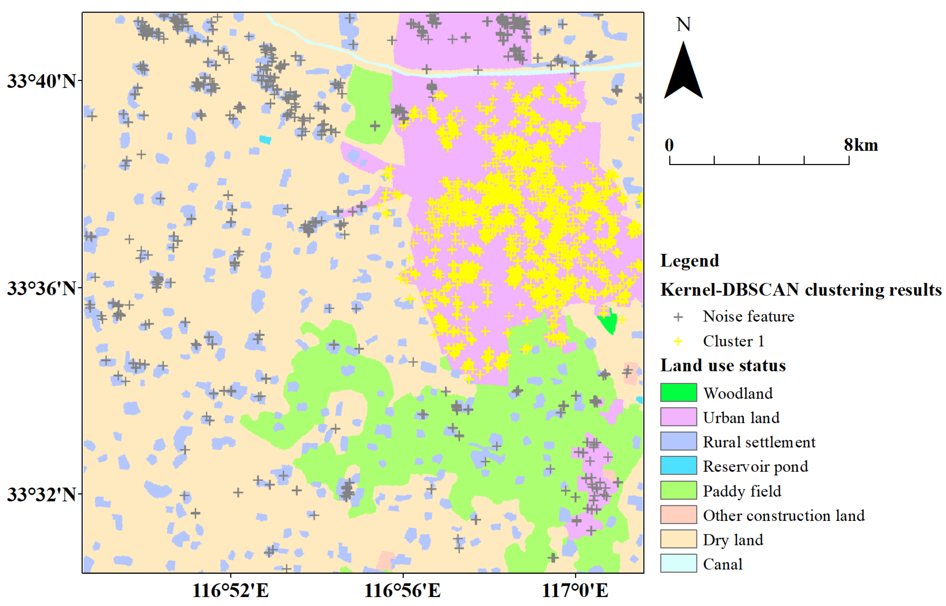
5.1. Kernel-DBSCAN Clustering
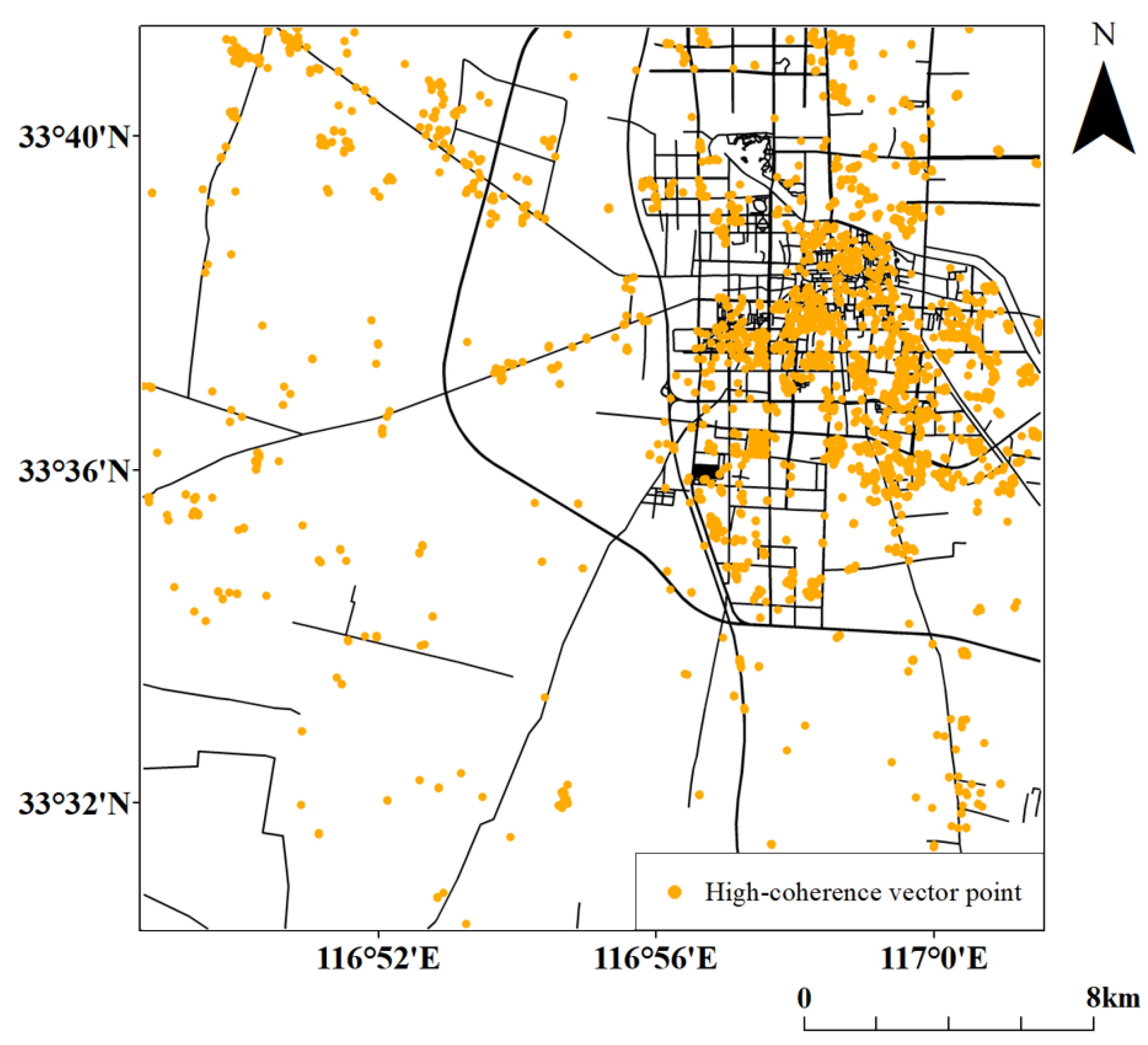
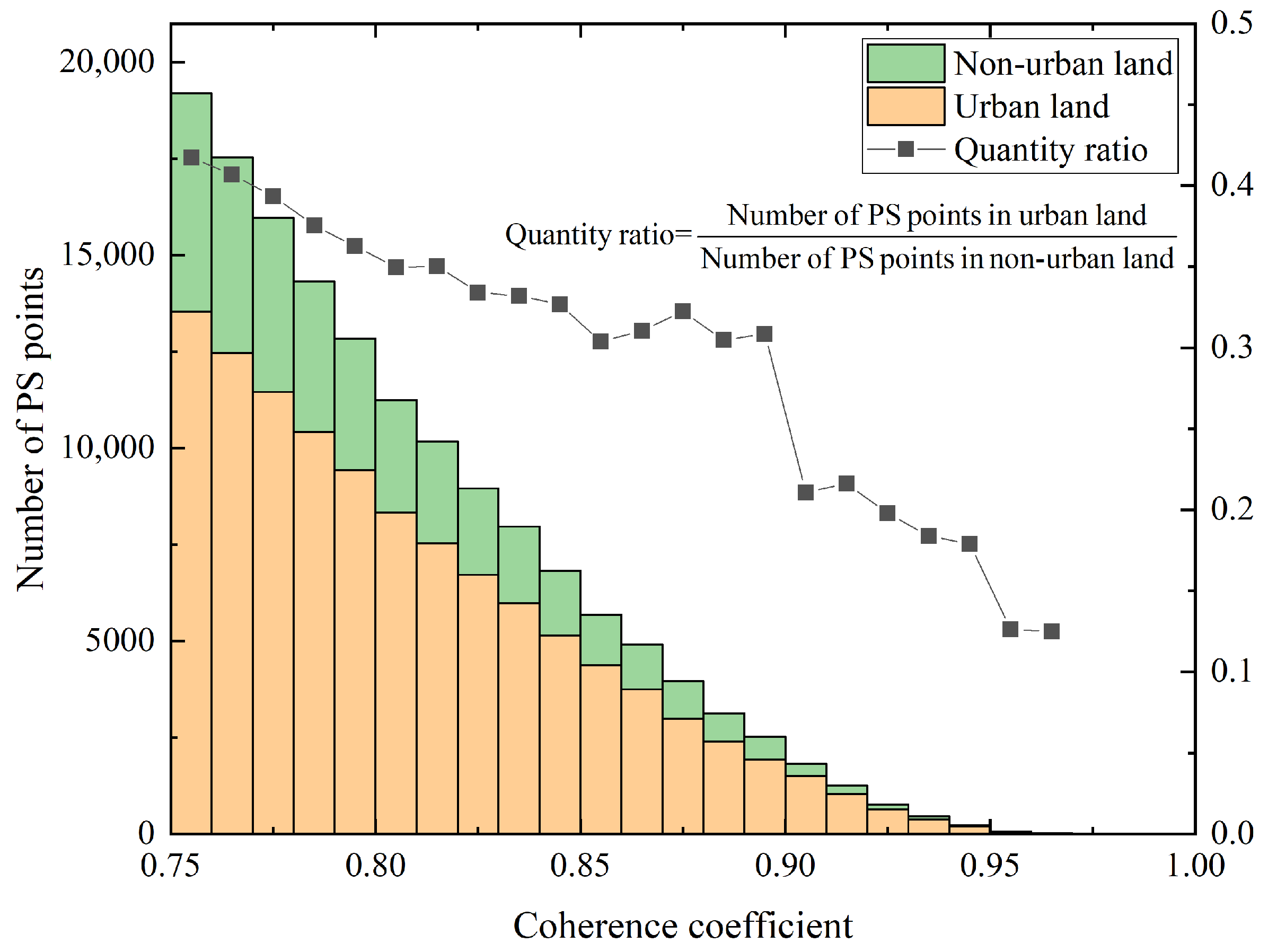
5.2. Statistics of Coherence Coefficient
5.3. Clustering Analysis
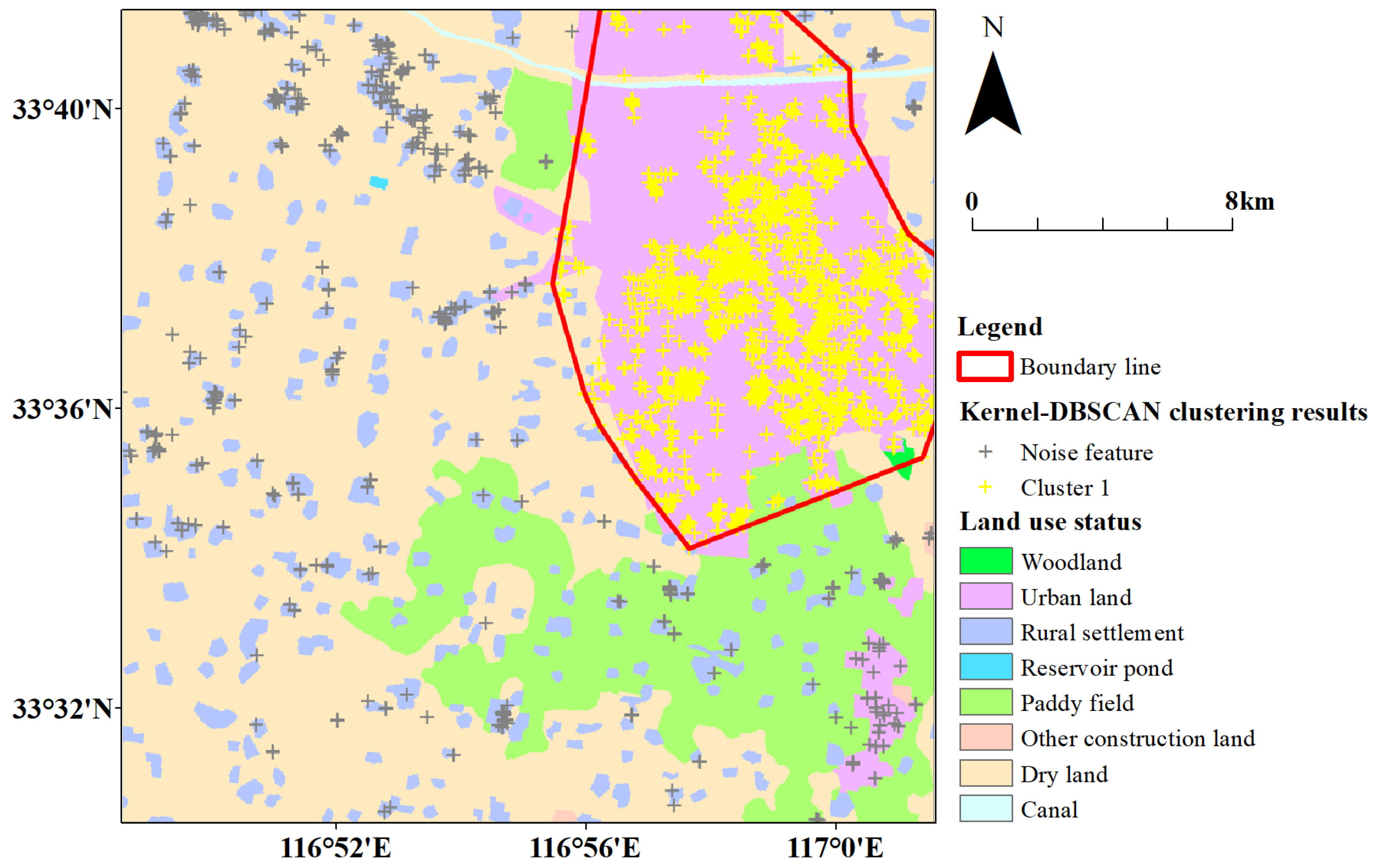
5.4. Boundaries Fusion
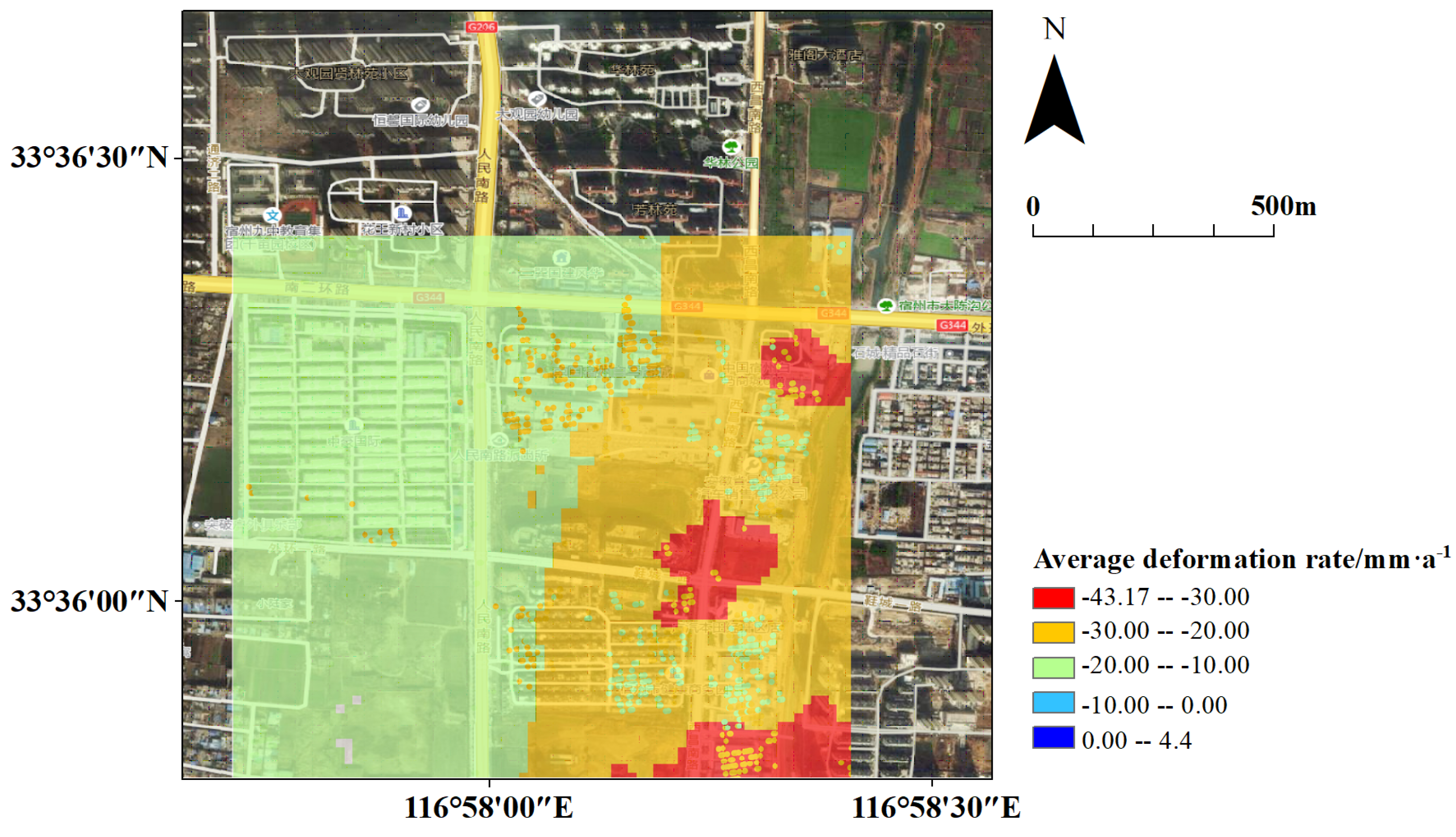
5.5. Data Fusion Results
6. Discussion
7. Conclusions
Author Contributions
Funding
Data Availability Statement
Acknowledgments
Conflicts of Interest
References
- Massonnet, D.; Feigl, K.L. Radar interferometry and its application to changes in the Earth’s surface. Rev. Geophys. 1998, 36, 441–500. [Google Scholar] [CrossRef] [Green Version]
- Hooper, A. A multi-temporal InSAR method incorporating both persistent scatterer and small baseline approaches. Geophys. Res. Lett. 2008, 35, 96–106. [Google Scholar] [CrossRef] [Green Version]
- Reinisch, E.; Cardiff, M.; Feigl, K. Graph theory for analyzing pair-wise data: Application to geophysical model parameters estimated from interferometric synthetic aperture radar data at Okmok volcano, Alaska. J. Geod. 2017, 91, 9–24. [Google Scholar] [CrossRef] [PubMed] [Green Version]
- Armaş, I.; Mendes, D.; Popa, R.G. Long-term ground deformation patterns of Bucharest using multi-temporal InSAR and multivariate dynamic analyses: A possible transpressional system? Sci. Rep. 2017, 7, 43762. [Google Scholar] [CrossRef] [PubMed] [Green Version]
- Werner, W.; Freysteinn, S.; Stéphanie, D.; Lavallée, Y. Post-emplacement cooling and contraction of lava flows: InSAR observations and a thermal model for lava felds at Hekla volcano, Iceland. J. Geophys. Res. Solid Earth 2017, 122, 946–965. [Google Scholar] [CrossRef] [Green Version]
- Foroughnia, F.; Nemati, S.; Maghsoudi, Y.; Perissin, D. An iterative PS-InSAR method for the analysis of large spatio-temporal baseline data stacks for land subsidence estimation. Int. J. Appl. Earth Obs. Geoinf. 2019, 74, 248–258. [Google Scholar] [CrossRef]
- Luo, H.B.; Li, Z.H.; Chen, J.J.; Pearson, C.; Wang, M.M.; Lv, W.C.; Ding, H.Y. Integration of Range Split Spectrum Interferometry and conventional InSAR to monitor large gradient surface displacements. Int. J. Appl. Earth Obs. Geoinf. 2019, 74, 130–137. [Google Scholar] [CrossRef] [Green Version]
- Zhao, K.; Wang, Q.; Zhuang, H.; Li, Z.; Chen, G. A fully coupled flow deformation model for seismic site response analyses of liquefiable marine sediments. Ocean Eng. 2022, 251, 111144. [Google Scholar] [CrossRef]
- Ferretti, A.; Prati, C.; Rocca, F. Permanent scatterers in SAR interferometry. IEEE Trans. Geosci. Remote Sens. 2001, 39, 8–20. [Google Scholar] [CrossRef]
- Hooper, A.; Segall, P.; Zebker, H.A. Persistent scatterer interferometric synthetic aperture radar for crustal deformation analysis, with application to Volcan Alcedo, Galapagos. J. Geophys. Res. Solid Earth 2007, B07407, 112. [Google Scholar] [CrossRef] [Green Version]
- Hooper, A.; Zebker, H.; Segall, P.; Kampes, B. A new method for measuring deformation on volcanoes and other natural terrains using InSAR persistent scatterers. Geophys. Res. Lett. 2004, 31, 1–5. [Google Scholar] [CrossRef]
- Berardino, P.; Fornaro, G.; Lanari, R.; Sansosti, E. A New Algorithm for Surface Deformation Monitoring Based on Small Baseline Differential SAR Interferograms. IEEE Trans. Geosci. Remote Sens. 2002, 40, 2375–2383. [Google Scholar] [CrossRef] [Green Version]
- Usai, S. A least squares database approach for SAR interferometric data. IEEE Trans. Geosci. Remote Sens. 2003, 41, 753–760. [Google Scholar] [CrossRef] [Green Version]
- Colesanti, C.; Wasowski, J. Investigating landslides with space-borne Synthetic Aperture Radar (SAR) interferometry. Eng. Geol. 2006, 88, 173–199. [Google Scholar] [CrossRef]
- López-Quiroz, P.; Doin, M.P.; Tupin, F.; Briole, P.; Nicolas, J.M. Time series analysis of Mexico City subsidence constrained by radar interferometry. J. Appl. Geophys. 2009, 69, 1–15. [Google Scholar] [CrossRef]
- Hetland, E.A.; Musã, P.; Simons, M.; Lin, Y.N.; Agram, P.S.; Dicaprio, C.J. Multiscale InSAR Time Series (MInTS) analysis of surface deformation. J. Geophys. Res. 2012, 117, 1–17. [Google Scholar] [CrossRef] [Green Version]
- Chen, M.; Tomás, R.; Li, Z.; Motagh, M.; Li, T.; Hu, L.; Gong, H.; Li, X.; Yu, J.; Gong, X. Imaging land subsidence induced by groundwater extraction in Beijing (China) using satellite radar interferometrys. Remote Sens. 2016, 8, 468. [Google Scholar] [CrossRef] [Green Version]
- Motagh, M.; Shamshiri, R.; Haghighi, M.H. Quantifying groundwater exploitation induced subsidence in the Rafsanjan plain, southeastern Iran, using InSAR time-series and in situ measurements. Eng. Geol. 2017, 218, 134–151. [Google Scholar] [CrossRef]
- Darvishi, M.; Destouni, G.; Aminjafari, S.; Jaramillo, F. Multi-Sensor InSAR Assessment of Ground Deformations around Lake Mead and Its Relation to Water Level Changes. Remote Sens. 2021, 13, 406. [Google Scholar] [CrossRef]
- Samsonov, S.; Dille, A.; Dewitte, O.; Kervyn, F.; d’Oreye, N. Satellite interferometry for mapping surface deformation time series in one, two and three dimensions: A new method illustrated on a slow-moving landslide. Eng. Geol. 2020, 266, 105471. [Google Scholar] [CrossRef]
- Maghsoudi, Y.; van der Meer, F.; Hecker, C.; Perissin, D.; Saepuloh, A. Using PS-InSAR to detect surface deformation in geothermal areas of West Java in Indonesia. Int. J. Appl. Earth Obs. Geoinf. 2018, 64, 386–396. [Google Scholar] [CrossRef]
- Jiang, C.; Fan, W.; Yu, N.; Nan, Y. A New Method to Predict Gully Head Erosion in the Loess Plateau of China Based on SBAS-InSAR. Remote Sens. 2021, 13, 421. [Google Scholar] [CrossRef]
- Shanker, P.; Casu, F.; Zebker, H.A.; Lanari, R. Comparison of Persistent Scatterers and Small Baseline Time-Series InSAR Results: A Case Study of the San Francisco Bay Area. IEEE Geosci. Remote Sens. Lett. 2011, 8, 592–596. [Google Scholar] [CrossRef]
- Crosetto, M.; Monserrat, O.; Cuevas-Gonzalez, M.; Devanthery, N.; Crippa, B. Persistent Scatterer Interferometry: A review. ISPRS J. Photogramm. Remote Sens. 2016, 115, 78–89. [Google Scholar] [CrossRef] [Green Version]
- Miranda, S.; Hernández-Madrigal, V.; Tuxpan-Vargas, J.; Reyes, C. Evolution assessment of structurally-controlled differential subsidence using SBAS and PS interferometry in an emblematic case in Central Mexico. Eng. Geol. 2020, 279, 105860. [Google Scholar] [CrossRef]
- Chen, Y.; Yu, S.; Tao, Q.; Liu, G.; Wang, L.; Wang, F. Accuracy Verification and Correction of D-InSAR and SBAS-InSAR in Monitoring Mining Surface Subsidence. Remote Sens. 2021, 13, 4365. [Google Scholar] [CrossRef]
- Umarhadi, D.; Avtar, R.; Widyatmanti, W.; Johnson, B.; Yunus, A.; Khedher, K.; Singh, G. Use of multifrequency (C-band and L-band) SAR data to monitor peat subsidence based on time-series SBAS InSAR technique. Land Degrad. Dev. 2021, 32, 7. [Google Scholar] [CrossRef]
- Tao, Q.; Wang, F.; Guo, Z.; Hu, L.; Yang, C.; Liu, T. Accuracy verification and evaluation of small baseline subset (SBAS) interferometric synthetic aperture radar (InSAR) for monitoring mining subsidence. Eur. J. Remote Sens. 2021, 54, 642–663. [Google Scholar] [CrossRef]
- Aslan, G.; Foumelis, M.; Raucoules, D.; Michele, M.D.; Bernardie, S.; Cakir, Z. Landslide mapping and monitoring using persistent scatterer interferometry (PSI) technique in the French Alps. Remote Sens. 2021, 12, 1305. [Google Scholar] [CrossRef] [Green Version]
- Tarighat, F.; Foroughnia, F.; Perissin, D. Monitoring of Power Towers’ Movement Using Persistent Scatterer SAR Interferometry in South West of Tehran. Remote Sens. 2021, 13, 407. [Google Scholar] [CrossRef]
- Guo, C.B.; Yan, Y.Q.; Zhang, Y.S.; Zhang, X.J.; Zheng, Y.Z.; Li, X.; Yang, Z.H.; Wu, R. Study on the Creep-Sliding Mechanism of the Giant Xiongba Ancient Landslide Based on the SBAS-InSAR Method, Tibetan Plateau, China. Remote Sens. 2021, 13, 3365. [Google Scholar] [CrossRef]
- Liu, L.M.; Yu, J.; Chen, B.B.; Wang, Y.B. Urban subsidence monitoring by SBAS-InSAR technique with multi-platform SAR images: A case study of Beijing Plain, China. Eur. J. Remote Sens. 2020, 53, 2279–7254. [Google Scholar] [CrossRef] [Green Version]
- Wu, Q.; Jia, C.T.; Chen, S.B.; Li, H.Q. SBAS-InSAR Based Deformation Detection of Urban Land, Created from Mega-Scale Mountain Excavating and Valley Filling in the Loess Plateau: The Case Study of Yan’an City. Remote Sens. 2019, 11, 1673. [Google Scholar] [CrossRef] [Green Version]
- Darwish, N.; Kaiser, M.; Koch, M.; Gaber, A. Assessing the accuracy of ALOS/PALSAR-2 and sentinel-1 radar images in estimating the land subsidence of coastal areas: A case study in Alexandria city, Egypt. Remote Sens. 2021, 13, 1838. [Google Scholar] [CrossRef]
- He, Y.; Xu, G.; Kaufmann, H.; Wang, J.; Ma, H.; Liu, T. Integration of InSAR and LiDAR Technologies for a Detailed Urban Subsidence and Hazard Assessment in Shenzhen, China. Remote Sens. 2021, 13, 2336. [Google Scholar] [CrossRef]
- Cigna, F.; Esquivel Ramírez, R.; Tapete, D. Accuracy of Sentinel-1 PSI and SBAS InSAR Displacement Velocities against GNSS and Geodetic Leveling Monitoring Data. Remote Sens. 2021, 13, 4800. [Google Scholar] [CrossRef]


| Satellite Sensor | Orbit | Revisit Period/d | Wave Band | Wavelength/cm | Incident Angle/° | Resolution Ratio/m |
|---|---|---|---|---|---|---|
| Sentinel-1A | Sun synchronous satellite | 12 | C | 5.6 | 38.9 | 5 × 20 |
| Month | 1 | 2 | 3 | 4 | 5 | 6 | 7 | 8 | 9 | 10 | 11 | 12 | ||
|---|---|---|---|---|---|---|---|---|---|---|---|---|---|---|
| Day | ||||||||||||||
| Year | ||||||||||||||
| 2017 | / | / | / | / | / | 25 | 19 | 24 | 17 | 23 | 28 | 22 | ||
| 2018 | 27 | 20 | 28 | 21 | 27 | 20 | 26 | 19 | 24 | 18 | 23 | 29 | ||
| 2019 | 22 | 27 | 23 | 28 | 22 | 27 | 21 | 26 | 19 | 25 | 30 | 24 | ||
| 2020 | 17 | 22 | 29 | 22 | 28 | 21 | 27 | / | / | / | / | / | ||
| Point | PS-InSAR Cumulative Settlement Monitoring Value/mm | SBAS-InSAR Cumulative Settlement Monitoring Value/mm | Cumulative Settlement Monitoring Value Deviation/mm | Average Annual Subsidence Rate Deviation/(mm·a ) |
|---|---|---|---|---|
| a | −69.5 | −61.4 | −8.1 | −2.5 |
| b | −53.1 | −59.2 | 6.1 | 1.9 |
| c | −38.5 | −37.5 | −1.1 | −0.3 |
| d | −31.5 | −49.4 | 17.9 | 5.7 |
| e | −40.8 | −34.6 | −6.2 | −1.9 |
| Maximum Side | Overlap Rate | |||
|---|---|---|---|---|
| 1 | – | 115,403,348.94 | 138,519,186.10 | 83.31% |
| 2 | 6350.65 | 115,339,728.74 | 138,042,118.69 | 83.55% |
| 3 | 6046.70 | 115,128,944.82 | 136,211,030.91 | 84.52% |
| 4 | 4604.77 | 114,453,742.01 | 135,250,500.18 | 84.62% |
| 5 | 3727.83 | 111,474,879.95 | 132,154,035.59 | 84.35% |
Publisher’s Note: MDPI stays neutral with regard to jurisdictional claims in published maps and institutional affiliations. |
© 2022 by the authors. Licensee MDPI, Basel, Switzerland. This article is an open access article distributed under the terms and conditions of the Creative Commons Attribution (CC BY) license (https://creativecommons.org/licenses/by/4.0/).
Share and Cite
Zhang, P.; Guo, Z.; Guo, S.; Xia, J. Land Subsidence Monitoring Method in Regions of Variable Radar Reflection Characteristics by Integrating PS-InSAR and SBAS-InSAR Techniques. Remote Sens. 2022, 14, 3265. https://doi.org/10.3390/rs14143265
Zhang P, Guo Z, Guo S, Xia J. Land Subsidence Monitoring Method in Regions of Variable Radar Reflection Characteristics by Integrating PS-InSAR and SBAS-InSAR Techniques. Remote Sensing. 2022; 14(14):3265. https://doi.org/10.3390/rs14143265
Chicago/Turabian StyleZhang, Peng, Zihao Guo, Shuangfeng Guo, and Jin Xia. 2022. "Land Subsidence Monitoring Method in Regions of Variable Radar Reflection Characteristics by Integrating PS-InSAR and SBAS-InSAR Techniques" Remote Sensing 14, no. 14: 3265. https://doi.org/10.3390/rs14143265
APA StyleZhang, P., Guo, Z., Guo, S., & Xia, J. (2022). Land Subsidence Monitoring Method in Regions of Variable Radar Reflection Characteristics by Integrating PS-InSAR and SBAS-InSAR Techniques. Remote Sensing, 14(14), 3265. https://doi.org/10.3390/rs14143265