
Extracting Urban Road Footprints from Airborne LiDAR Point Clouds with PointNet++ and Two-Step Post-Processing


Abstract
:1. Introduction
- (1)
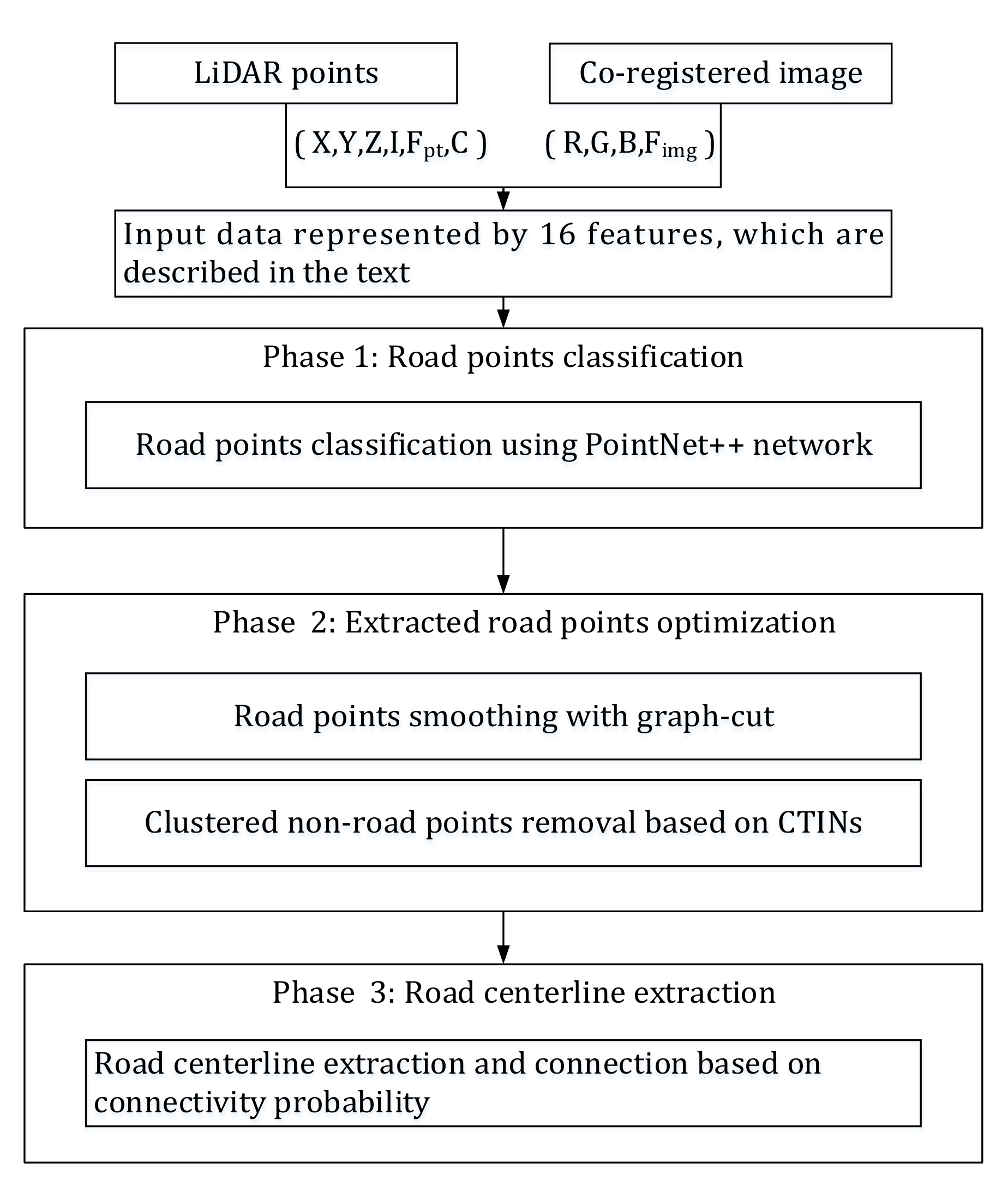
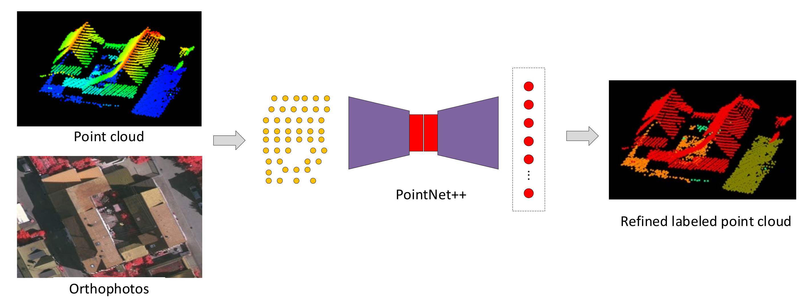
- Road points extraction by PointNet++, where the features of the input data include not only those selected from raw LiDAR points, such as 3D coordinate values, intensity, etc., but also the DN values of co-registered images and generated geometric features to describe a strip-like road.
- (2)
- Two-step post-processing of the extracted road points from PointNet++ by graph-cut and constrained triangulation irregular networks (CTINs) to smooth road points and to remove clustered non-road points.
- (3)
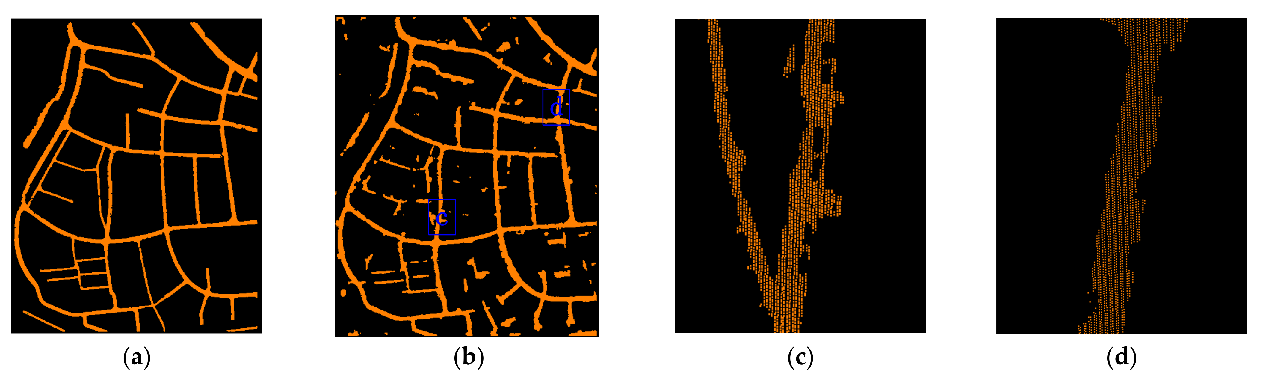
- Centerline extraction based on a modified method originally proposed in [21], where road segment gaps and holes caused by the occlusion of vehicles, trees, and buildings are recovered by estimating the connection probability of the road segment through collinearity and width similarity.
- (1)
- Strip-like descriptors are proposed to characterize the geometric property of a road, which can be applied to both point clouds and optical images. Strip-like descriptors, together with other features, are input to the PointNet++ network, resulting in a more accurate road point classification.
- (2)
- Collinearity and width similarity are proposed to estimate the connection probability of road segments to repair the road gaps and holes caused by the occlusion of vehicles, trees, buildings, and some omission errors.
2. Materials and Method
2.1. Sample Materials
2.2. Method
2.2.1. Overview of Method
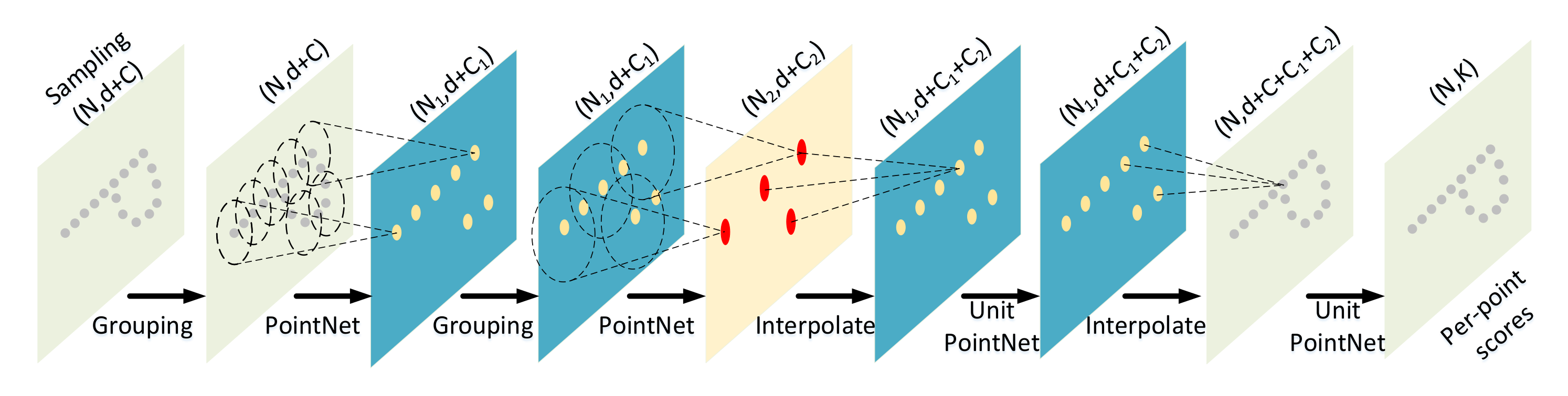
2.2.2. Road Points Classification
- (1)
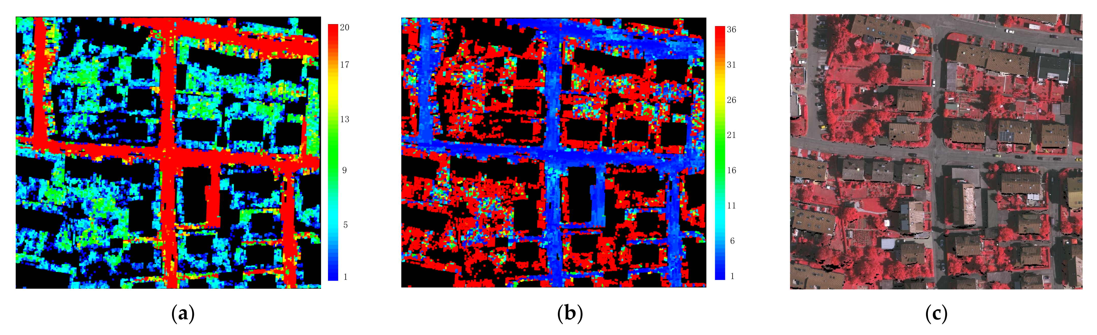
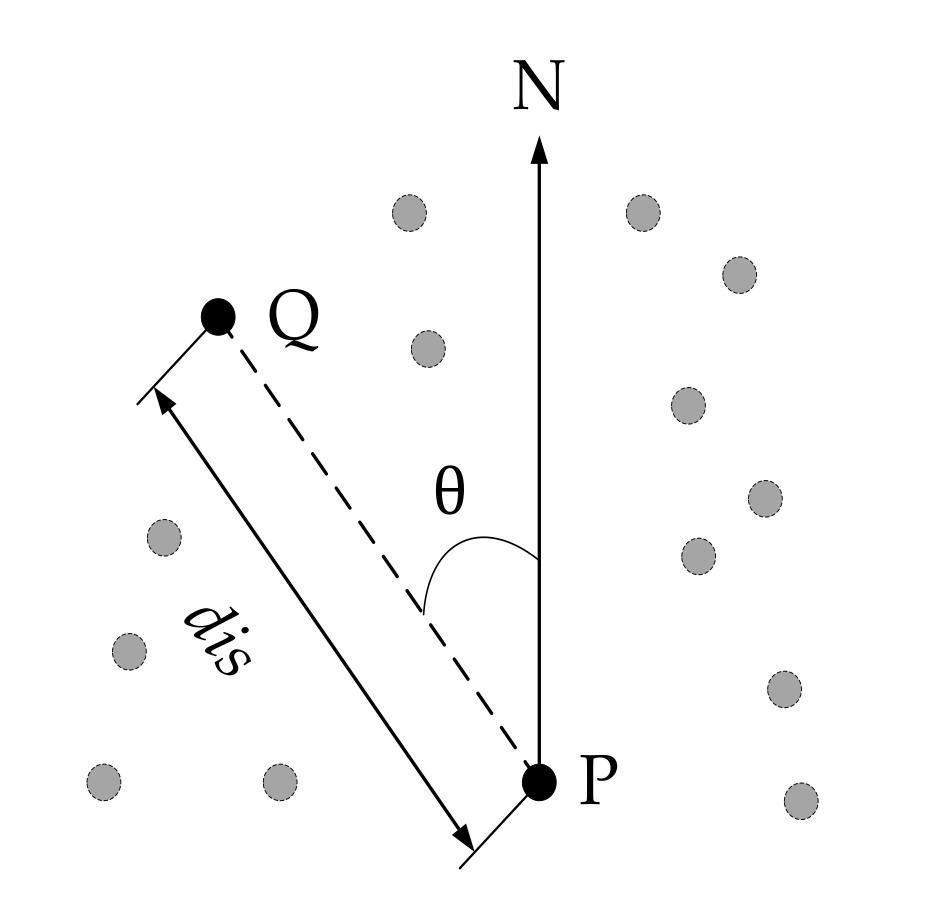
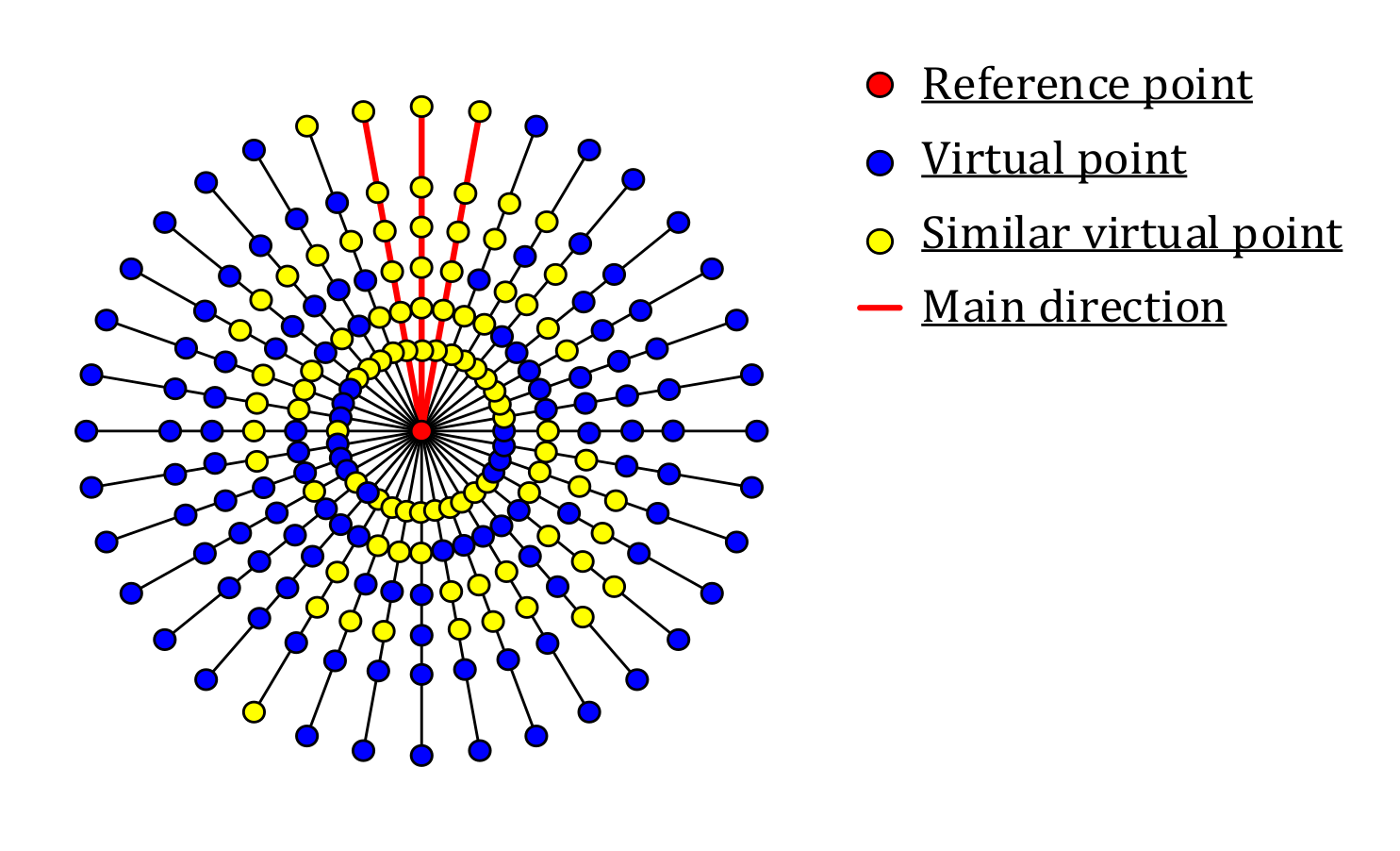
- Generate the virtual point set of the current reference point by Formula (1), where . The direction is defined as the direction where P points to North. The increase of θ by can reduce computation load while ensuring the accuracy of strip descriptors [21].
- (2)
- Calculate the average intensity value of each virtual point. Select a virtual point from the virtual point set . Search the k-neighborhood points on the projected LiDAR points of , and assign the average intensity of all points in the neighborhood to the intensity value of . To guarantee that each virtual point from the road contains at least one neighborhood point, the value of k is 2 times the average point spacing. In cases where a virtual point contains no neighborhood points, its intensity value is set to −1, indicating an invalid point.
- (3)
- Calculate the intensity difference between each virtual point and the reference point and mark the virtual points with an intensity difference lower than a given threshold as similar virtual points. Count the number of consecutive similar virtual points starting from the reference point in 36 directions from , and denote them by . This step can be formulated as follows:where is the intensity value of the reference point and is the intensity value of the virtual point at the distance in the direction with regard to the reference point. is the intensity difference threshold, and, as noted in [20], the range of road intensity difference in a local road area is around -15 ~ +15 if the road is paved with the same material, so the absolute value of is set to 15 for the data sets tested in this study. “” is used to mark the similar virtual points. Therefore, the number of consecutive similar virtual points in any direction can be counted by the following steps:
- Set the initial values of to 0.
- Set the initial direction ω to , denote the virtual points in this direction by , where the points are sequenced by the increasing distance from the virtual points and the reference point.
- For a given point from , if its corresponding , then go to the next point and add 1 to . Otherwise, stop the counting for this direction, set , and go to step b.
- Repeat the steps until .
- (4)
- Suppose is the main direction of P, which, according to the definition of the main direction, is the direction with the largest number of consecutive similar virtual points. Let be the number of continuous similar virtual points in the ε direction. Iteratively calculate the difference between and , record them as , which can be expressed as:
- Rotate from the main direction counterclockwise, every 10, to check whether is less than the given threshold where subscript or if . If it is true and , then,Otherwise, if , or , continue to the next step.
- Rotate from the main direction clockwise, every 10, to check whether is less than the given threshold where subscript or if . If it is true and , then,Otherwise, if , or , continue to the final step.
2.2.3. Two-Step Post-Processing of Initial Road Points
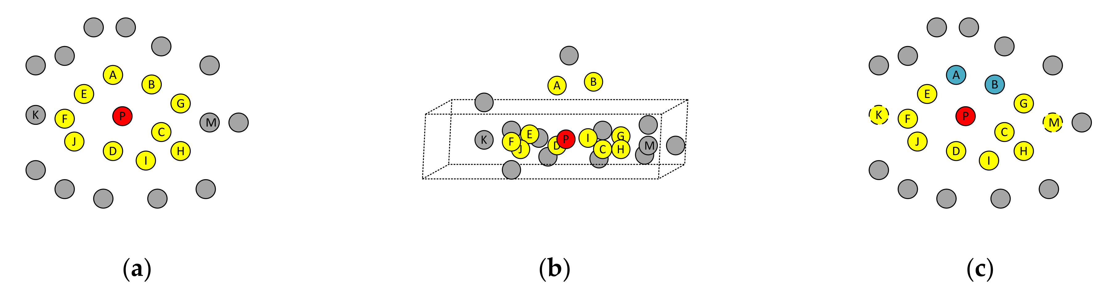
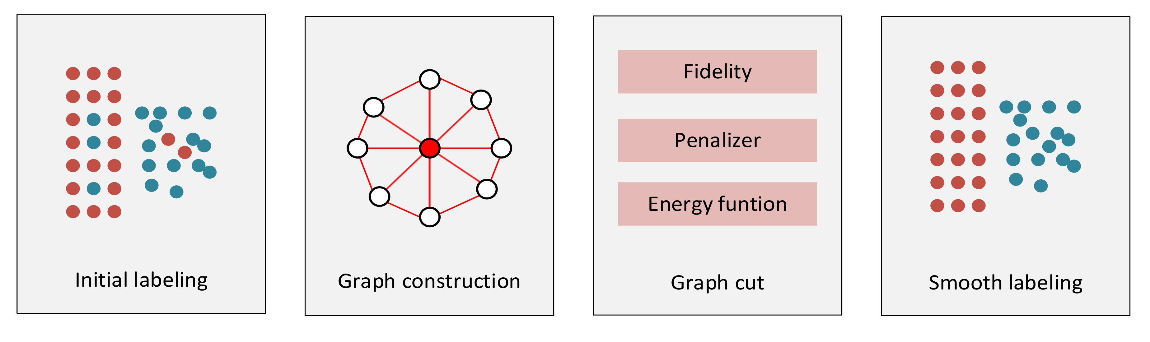
Road Point Smoothing with Graph-Cut
Clustered Non-Road Points Removal Based on CTINs
- (1)
- The Bower–Watson algorithm [47] is applied to construct the Delaunay triangulation of the graph-cut processed initial road points.
- (2)
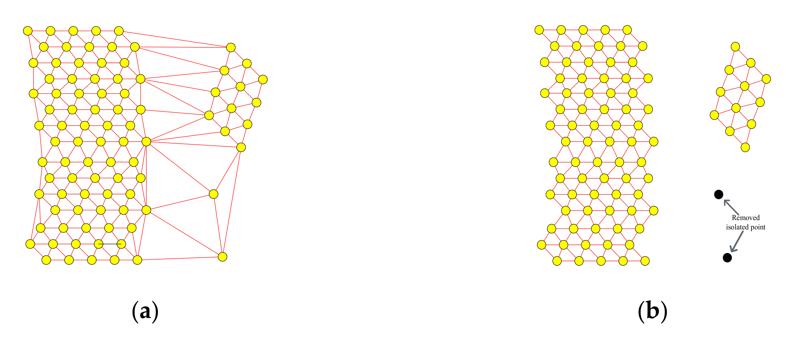
- Traverse the edges of the triangles and remove the edges with lengths greater than , which is set to twice the mean average point spacing in the raw point clouds. Figure 13 shows the triangles before and after this step is performed.
- (3)
- Remove isolated points, resulting in separated clusters of triangles, as shown in Figure 13b.
- (4)
- Calculate the total area of individual clusters of triangles obtained in step 3. Remove those clusters with areas less than a given threshold , which is the minimum area of a road in the urban setting. The empirical value of Ts for urban areas is 100 m2.The total area of clustered triangles can be calculated as follows: the points constructed from the triangles are projected onto the x-y plane. Their maximum and minimum X, Y values, which are denoted by , , and , respectively, are obtained. A rectangle can be formed by them. Grid the rectangle with the cell size of . Count all cells with at least one point inside and then sum up the area of these cells, which is the approximation of the total area of the clustered triangles. We used this approximation method rather than calculating the area of individual triangles, and then summed them up to reduce computational load.
- (5)
- For the remaining clusters of triangles, the minimum bounding rectangle (MBR) method proposed in [48] was used to form a bounding rectangle for each cluster. Denote the length, width and area of the rectangle by , and . Calculate aspect ratio and point coverage as follows:where is the area of a given triangle cluster calculated in step 4. If > and > , where , are two predefined thresholds, then remove the cluster and all points inside. The values of and are 6 and 0.3, respectively, which are based on prior knowledge acquired by inspecting these parameters in a given urban region.
2.2.4. Road Centerlines Extraction
- (1)
- First, define the connection range. To prevent connecting two lines that are far apart, a radius R is defined to determine the connection range. If the distance between the endpoints of two road segments is greater than R, the connection probability of the two lines sets to 0. The value of R is set to the width of the smallest residential block in the study area, which is 50 m in the testing region.
- (2)
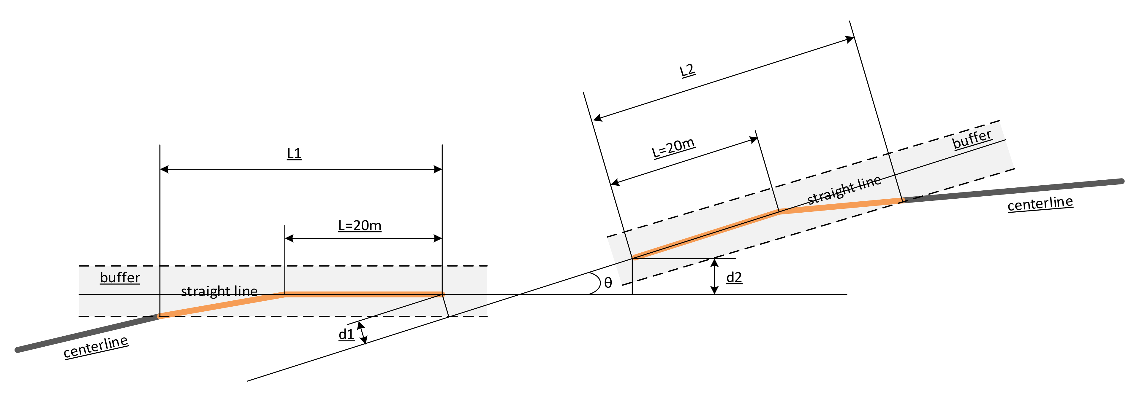
- Collinearity (): A road with enough length may be curve in some part, which can change the extension direction of the road at the endpoints. To keep the true extension direction, a segment with length L at the end part of a road is selected to fit a straight line, as shown in Figure 15. A too-small value of L causes a large deviation between the direction of the fitted straight line and the actual direction, while a too-large L value may include the curved part of the road in the straight fitted line. It was set to 20 m in the study, by trial-and-error, which may be set as a constant parameter if similar studies are performed. Then, collinearity is defined by the following formula:where, and are the distances from one end of a road to another fitted straight line (see Figure 15). is the angle between the two fitted straight lines. and are the lengths of the matched lines. A matched line is defined as follows: create the buffer zone of a fitted straight line. Project the road segment surrounded by the buffer zone onto the direction of the fitted straight line, then is the length of the projected segment. The buffer width is half the largest road width in the studied area.
- (3)
- Width similarity is another parameter for calculating connection probability, which is defined by the following:where, and are the widths of the two road segments. is the difference between the possible largest and smallest widths of roads in study area.
- (4)
- Connection probability of the two road segments can then be calculated by the following formula:where, and are the weights for collinearity measure and width similarity, respectively, both of which can be set to 0.5 if the two parameters are of similar importance. If the connection probability is greater than a given threshold , then the two road segments are connected.
2.3. Evaluation Metrics
3. Results
- (1)
- Input the raw point clouds directly to PointNet++ with each point represented by a 16D vector, described in Section 2. Six output classes are set to the PointNet++, namely, roads, public patches, buildings, and low, medium and tall vegetations. The result is denoted by M_class6.
- (2)
- The same input as (1) but only two outputs are set to the classifier: road points and non-road points; the result is denoted by M_class2.
- (3)
- Raw point clouds are firstly filtered by auto-adaptive progressive TIN proposed in [51] to obtain ground points, then input into PointNet++ to distinguish road and non-road points with and without the 9 strip descriptors, respectively; results are denoted by M_class2_from_ground_points and M_without_geometric_features.
- (1)
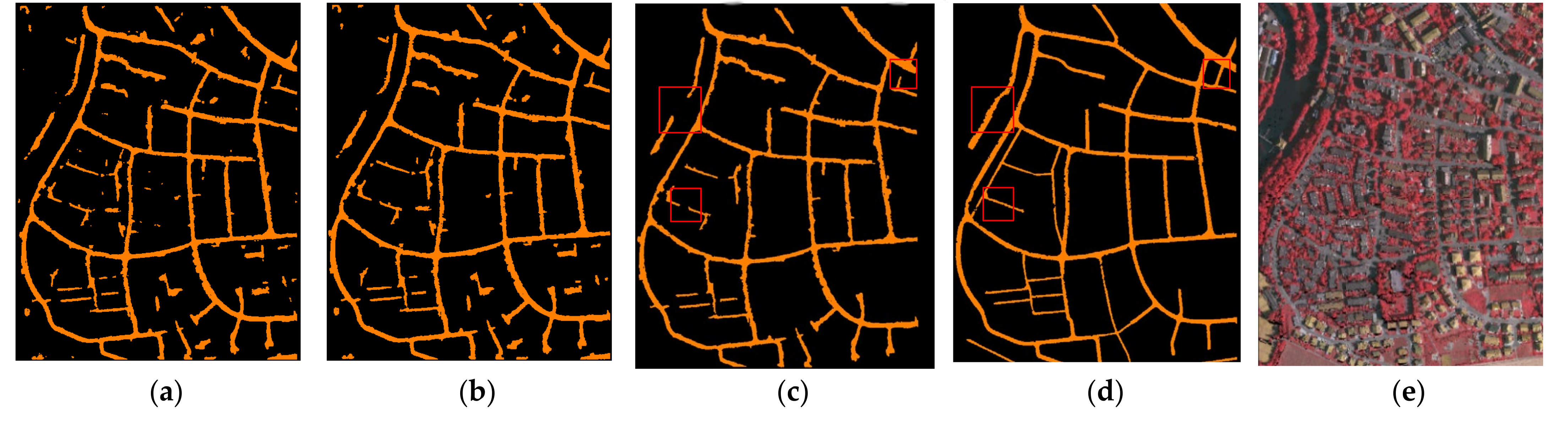
- The deep features learned by PointNet++ and the geometric features generated in the first phase of the framework jointly improved the completeness of the extracted road points.
- (2)
- Two-step post-processing is applied to decrease both omission and commission errors in the initial road points distinguished by PointNet++.
- (3)
- Collinearity and width similarity are introduced to calculate the connection probability to further improve the completeness of extracted roads.
4. Discussion
- (1)
- When the KNN search is applied to filter point clouds where only ground points (including road footprints) remained, the distance between a pair of points in the search region may be too large, resulting in useless features. That is, though the features can be generated, they are insignificant to the classifier or even decrease the classification accuracy.
- (2)
- When a fixed radius search is applied, some points may lack enough neighbor points for feature calculation, causing some feature loss.
5. Conclusions
Author Contributions
Funding
Acknowledgments
Conflicts of Interest
References
- Kobler, A.; Pfeifer, N.; Ogrinc, P.; Todorovski, L.; Oštir, K.; Džeroski, S. Repetitive interpolation: A robust algorithm for DTM generation from aerial laser scanner data in forested terrain. Remote Sens. Environ. 2007, 108, 9–23. [Google Scholar] [CrossRef]
- Polat, N.; Uysal, M. Investigating performance of airborne LiDAR data filtering algorithms for DTM generation. Measurement 2015, 63, 61–68. [Google Scholar] [CrossRef]
- Ma, H.; Ma, H.; Liu, K.; Luo, W.; Zhang, L. Direct georeferencing for the images in an airborne LiDAR system by automatic boresight misalignments calibration. Sensors 2020, 20, 5056. [Google Scholar] [CrossRef] [PubMed]
- Meng, X.; Wang, L.; Currit, N. Morphology-based building detection from airborne LiDAR data. Photogramm. Eng. Remote Sens. 2009, 75, 437–442. [Google Scholar] [CrossRef]
- Hamraz, H.; Jacobos, N.B.; Contreras, M.A.; Clark, C.H. Deep learning for conifer/deciduous classification of airborne LiDAR 3D point clouds representing individual trees. ISPRS J. Photogramm. 2019, 158, 219–230. [Google Scholar] [CrossRef] [Green Version]
- Axelsson, P. DEM generation from laser scanner data using adaptive TIN models. Int. Arch. Photogramm. Remote Sens. 2000, 33, 110–118. [Google Scholar]
- Hatger, C.; Brenner, C. Extraction of road geometry parameters from laser scanning and existing databases. Int. Arch. Photogramm. Remote Sens. Spatial Inf. Sci. 2003, 34, 225–230. [Google Scholar]
- Jia, J.; Sun, H.; Jiang, C.; Karila, K.; Karjalainen, M.; Ahokas, E.; Khoramshahi, E.; Hu, P.; Chen, C.; Xue, T.; et al. Review on active and passive remote sensing techniques for road extraction. Remote Sens. 2021, 13, 4235. [Google Scholar] [CrossRef]
- Rottensteiner, F.; Clode, S. Building and road extraction by LiDAR and imagery. In Topographic Laser Ranging and Scanning: Principles and Processing; CRC Press: Boca Raton, FL, USA, 2008; pp. 445–478. [Google Scholar] [CrossRef]
- Ma, H.; Zhou, W.; Zhang, L.; Wang, S. Decomposition of small-footprint full waveform LiDAR data based on generalized Gaussian model and grouping LM optimization. Meas. Sci. and Technol. 2017, 28, 1–9. [Google Scholar] [CrossRef]
- Tolt, G.; Shimoni, M.; Ahlberg, J. A shadow detection method for remote sensing images using VHR hyperspectral and LiDAR data. In Proceedings of the IEEE International Geoscience and Remote Sensing Symposium IGARSS, Vancouver, BC, Canada, 24–29 July 2011; pp. 4423–4426. [Google Scholar] [CrossRef]
- Rieger, W.; Kerschner, M.; Reiter, T.; Rottensteiner, F. Roads and buildings from laser scanner data within a forest enterprise. Int. Arch. Photogramm. Remote Sens. 1999, 32, 642–649. [Google Scholar]
- Clode, S.; Kootsookos, P.J.; Rottensteiner, F. The automatic extraction of roads from LiDAR data. Int. Arch. Photogramm. Remote Sens. Spatial Inf. Sci. 2004, 35, 231–237. [Google Scholar]
- Clode, S.; Rottensteiner, F.; Kootsookos, P.; Zelniker, E. Detection and vectorization of roads from LiDAR data. Photogramm. Eng. Remote Sens. 2007, 73, 517–535. [Google Scholar] [CrossRef] [Green Version]
- Choi, Y.W.; Jang, Y.W.; Lee, H.J.; Cho, G.S. Three-dimensional LiDAR data classifying to extract road point in urban area. IEEE Geosci. Remote Sens. Lett. 2008, 5, 725–729. [Google Scholar] [CrossRef]
- Samadzadegan, F.; Hahn, M.; Bigdeli, B. Automatic road extraction from LiDAR data based on classifier fusion. In Proceedings of the Joint Urban Remote Sensing Event (JURSE), Shanghai, China, 20–22 May 2009; pp. 1–6. [Google Scholar] [CrossRef]
- Zhu, Q.; Mordohai, P. A minimum cover approach for extracting the road network from airborne LiDAR data. In Proceedings of the International Conference on Computer Vision (ICCV) Workshops, Kyoto, Japan, 27 September–4 October 2009; pp. 1582–1589. [Google Scholar] [CrossRef]
- Zhao, J.; You, S. Road network extraction from airborne LiDAR data using scene context. In Proceedings of the Conference on Computer Vision and Pattern Recognition Workshops (CVPRW) Workshops, Providence, RI, USA, 16–21 June 2012; pp. 9–16. [Google Scholar] [CrossRef]
- Matkan, A.A.; Hajeb, M.; Sadeghian, S. Road extraction from LiDAR data using support vector machine classification. Photogramm. Eng. Remote Sens. 2014, 80, 409–422. [Google Scholar] [CrossRef] [Green Version]
- Li, Y.; Yong, B.; Wu, H.; An, R.; Xu, H. Road detection from airborne LiDAR point clouds adaptive for variability of intensity data. Optik 2015, 126, 4292–4298. [Google Scholar] [CrossRef]
- Hui, Z.; Hu, Y.; Jin, S.; Yevenyo, Y.Z. Road centerline extraction from airborne LiDAR point cloud based on hierarchical fusion and optimization. ISPRS J. Photogramm. 2016, 118, 22–36. [Google Scholar] [CrossRef]
- Husain, A.; Vaishya, R.C. Road surface and its center line and boundary lines detection using terrestrial LiDAR data. The Egypt. J. Remote Sens. Space Sci. 2018, 21, 363–374. [Google Scholar] [CrossRef]
- Chen, Z.; Liu, C.; Wu, H. A higher-order tensor voting-based approach for road junction detection and delineation from airborne LiDAR data. ISPRS J. Photogramm. 2019, 150, 91–114. [Google Scholar] [CrossRef]
- Zhu, P.; Lu, Z.; Chen, X.; Honda, K.; Eiumnoh, A. Extraction of city roads through shadow path reconstruction using laser data. Photogramm. Eng. Remote Sens. 2004, 70, 1433–1440. [Google Scholar] [CrossRef] [Green Version]
- Hu, X.; Tao, C.V.; Hu, Y. Automatic road extraction from dense urban area by integrated processing of high resolution imagery and LiDAR data. Int. Arch. Photogramm. Remote Sens. Spatial Inf. Sci. 2004, 35, 288–292. [Google Scholar]
- Youn, J.; Bethel, J.S.; Mikhail E., M. Extracting urban road networks from high-resolution true orthoimage and LiDAR. Photogramm. Eng. Remote Sens. 2008, 74, 227–237. [Google Scholar] [CrossRef]
- Wang, G.; Zhang, Y.; Li, J.; Song, P. 3D road information extraction from LiDAR data fused with aerial-images. In Proceedings of the IEEE International Conference on Data Mining (ICDM), Fuzhou, China, 29 June–1 July 2011; pp. 362–366. [Google Scholar] [CrossRef]
- Sameen, M.I.; Pradhan, B. A two-stage optimization strategy for fuzzy object-based analysis using airborne LiDAR and high-resolution orthophotos for urban road extraction. J. Sens. 2017, 2017, 1–17. [Google Scholar] [CrossRef] [Green Version]
- Milan, A. An integrated framework for road detection in dense urban area from high-resolution satellite imagery and LiDAR data. J. Geogr. Inf. Syst. 2018, 10, 175–192. [Google Scholar] [CrossRef] [Green Version]
- Nahhas, F.H.; Shafri, H.Z.M.; Sameen M., I.; Pradhan, B.; Mansor, S. Deep learning approach for building detection using LiDAR–orthophoto fusion. J. Sens. 2018, 2018, 1–13. [Google Scholar] [CrossRef] [Green Version]
- Maturana, D.; Scherer, S. VoxNet: A 3D convolutional neural network for real-time object recognition. In Proceedings of the IEEE International Workshop on Intelligent Robots and Systems (IROS), Hamburg, Germany, 28 September–2 October 2015; pp. 922–928. [Google Scholar] [CrossRef]
- Sun, Y.; Zhang, X.; Xin, Q.; Huang, J. Developing a multi-filter convolutional neural network for semantic segmentation using high-resolution aerial imagery and LiDAR data. ISPRS J. Photogramm. 2018, 143, 3–14. [Google Scholar] [CrossRef]
- Qi, C.R.; Su, H.; Mo, K.; Guibas, L.J. PointNet: Deep learning on point sets for 3D classification and segmentation. In Proceedings of the Conference on Computer Vision and Pattern Recognition (CVPR), Honolulu, HI, USA, 21–26 July 2017; pp. 77–85. [Google Scholar] [CrossRef] [Green Version]
- Qi, C.R.; Yi, L.; Su, H.; Guibas, L.J. PointNet++: Deep hierarchical feature learning on point sets in a metric space. In Proceedings of the 31st International Conference on Neural Information Processing Systems, Long Beach, CA, USA, 4–9 December 2017; pp. 1–10. [Google Scholar]
- Jiang, M.; Wu, Y.; Zhao, T.; Zhao, Z.; Lu, C. Pointsift: A siftlike network module for 3D point cloud semantic segmentation. arXiv 2018, arXiv:1807.00652. [Google Scholar]
- Zhao, H.; Jiang, L.; Fu, C.W.; Jia, J. PointWeb: Enhancing local neighborhood features for point cloud processing. In Proceedings of the IEEE conference on computer vision and pattern Recognition (CVPR), Long Beach, CA, USA, 15–20 June 2019; pp. 5565–5573. [Google Scholar] [CrossRef]
- Liu, H.; Guo, Y.; Ma, Y.; Lei, Y.; Wen, G. Semantic context encoding for accurate 3D point cloud segmentation. IEEE Trans. Multimedia 2021, 23, 2054–2055. [Google Scholar] [CrossRef]
- Feng, M.; Zhang, L.; Lin, X.; Gilani, S.Z.; Mian, A. Point attention network for semantic segmentation of 3D point clouds. Pattern Recognit. 2020, 107, 107446. [Google Scholar] [CrossRef]
- Hu, Q.; Yang, B.; Xie, L.; Rosa, S.; Guo, Y.; Wang, Z.; Trigoni, N.; Markham, A. RandLA-Net: Efficient semantic segmentation of large-scale point clouds. In Proceedings of the IEEE conference on computer vision and pattern Recognition (CVPR), Seattle, WA, USA, 13–19 June 2020; pp. 11105–11114. [Google Scholar] [CrossRef]
- Özdemir, E.; Remondino, F.; Golkar, A. Aerial point cloud classification with deep learning and machine learning algorithms. Int. Arch. Photogramm. Remote Sens. Spat. Inf. Sci. 2019, 42, 843–849. [Google Scholar] [CrossRef] [Green Version]
- Wen, C.; Li, X.; Yao, X.; Peng, L.; Chi, T. Airborne LiDAR point cloud classification with global-local graph attention convolution neural network. ISPRS J. Photogramm. 2021, 173, 181–194. [Google Scholar] [CrossRef]
- Hu, X.; Li, Y.; Shan, J.; Zhang, J.; Zhang, Y. Road centerline extraction in complex urban scenes from LiDAR data based on multiple features. IEEE Transact. Geosci. Remote Sens. 2014, 52, 7448–7456. [Google Scholar] [CrossRef]
- Huang, R.; Xu, Y.; Hong, D.; Yao, W.; Ghamisi, P.; Stilla, U. Deep point embedding for urban classification using ALS point clouds: A new perspective from local to global. ISPRS J. Photogramm. 2020, 163, 62–81. [Google Scholar] [CrossRef]
- Jing, Z.; Guan, H.; Zhao, P.; Li, D.; Yu, Y.; Zang, Y.; Wang, Y.; Wang, H.; Li, J. Multispectral LiDAR point cloud classification using SE-PointNet++. Remote Sens. 2021, 13, 2516. [Google Scholar] [CrossRef]
- Landrieu, L.; Raguet, H.; Vallet, B.; Mallet, C.; Weinmann, M. A structured regularization framework for spatially smoothing semantic labelings of 3D point clouds. ISPRS J. Photogramm. 2017, 132, 102–118. [Google Scholar] [CrossRef] [Green Version]
- Zhang, J.; Lin, X.; Ning, X. SVM-based classification of segmented airborne LiDAR point clouds in urban areas. Remote Sens. 2013, 5, 3749–3775. [Google Scholar] [CrossRef] [Green Version]
- Lee, J.; Dyczij-Edlinger, R. Automatic mesh generation using a modified Delaunay tessellation. IEEE Antennas Propagat. Magazine 1997, 39, 3445. [Google Scholar] [CrossRef]
- Kwak, E.; Habib, A. Automatic representation and reconstruction of DBM from LiDAR data using recursive minimum bounding rectangle. ISPRS J. Photogramm. 2014, 93, 171–191. [Google Scholar] [CrossRef]
- Heipke, C.; Mayer, H.; Wiedemann, C.; Jamet, O. Evaluation of automatic road extraction. Int. Arch. Photogramm. Remote Sens. 1997, 32, 172–187. [Google Scholar]
- Boyko, A.; Funkhouser, T. Extracting roads from dense point clouds in large scale urban environment. ISPRS J. Photogramm. 2011, 66, S2–S12. [Google Scholar] [CrossRef] [Green Version]
- Shi, X.; Ma, H.; Chen, Y.; Zhang, L.; Zhou, W. A parameter-free progressive TIN densification filtering algorithm for LiDAR point clouds. Int. J. Remote Sens. 2018, 39, 6969–6982. [Google Scholar] [CrossRef]


| Features | Symbol | Definition |
|---|---|---|
| Coordinate values | x, y, z | The coordinate values of a given point. |
| Intensity | I | The intensity of a given point. |
| Point density | The number of points per unit area. | |
| Strip descriptors for point clouds | are used to describe the length and main direction divergence (width) of a road in point clouds, see the text for details. | |
| Color | R, G, B | The DN values of a co-registered image. |
| Strip descriptors for optical image | ) are used to describe the length and main direction divergence (width) of a road in an image, see the text for details. |
| EC (%) | ECR (%) | Q (%) | ||
|---|---|---|---|---|
| PointNet++ | M_class6 | 76.2 | 74.0 | 60.1 |
| M_class2 | 79.8 | 73.9 | 62.3 | |
| M_class2_from_ground_points | 85.5 | 73.0 | 64.9 | |
| M_without_geometric_features | 82.7 | 71.0 | 61.9 | |
| Graph-cut smoothing | 85.6 | 73.0 | 65.0 | |
| Clustered non-road points removal | 84.7 | 79.7 | 69.6 | |
| Method | ECR (%) | EC (%) | Q (%) |
|---|---|---|---|
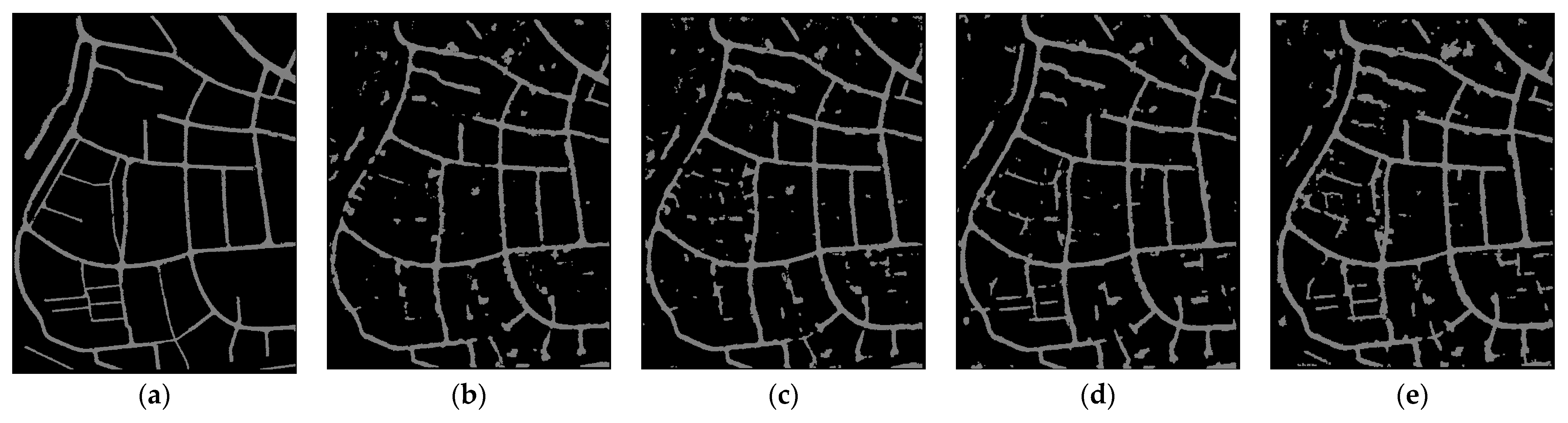
| PCD [14] | 53.2 | 58.3 | 38.5 |
| SRH [21] | 91.4 | 80.4 | 74.8 |
| MTH [42] | 73.8 | 53.4 | 44.9 |
| Proposed method | 97.0 | 86.3 | 84.1 |
| PD | 4.0 Points/m2 | 1.0 Points/m2 | 0.25 Points/m2 |
|---|---|---|---|
| RW | 2.0m | 3.0 m | 5.0m |
Publisher’s Note: MDPI stays neutral with regard to jurisdictional claims in published maps and institutional affiliations. |
© 2022 by the authors. Licensee MDPI, Basel, Switzerland. This article is an open access article distributed under the terms and conditions of the Creative Commons Attribution (CC BY) license (https://creativecommons.org/licenses/by/4.0/).
Share and Cite
Ma, H.; Ma, H.; Zhang, L.; Liu, K.; Luo, W. Extracting Urban Road Footprints from Airborne LiDAR Point Clouds with PointNet++ and Two-Step Post-Processing. Remote Sens. 2022, 14, 789. https://doi.org/10.3390/rs14030789
Ma H, Ma H, Zhang L, Liu K, Luo W. Extracting Urban Road Footprints from Airborne LiDAR Point Clouds with PointNet++ and Two-Step Post-Processing. Remote Sensing. 2022; 14(3):789. https://doi.org/10.3390/rs14030789
Chicago/Turabian StyleMa, Haichi, Hongchao Ma, Liang Zhang, Ke Liu, and Wenjun Luo. 2022. "Extracting Urban Road Footprints from Airborne LiDAR Point Clouds with PointNet++ and Two-Step Post-Processing" Remote Sensing 14, no. 3: 789. https://doi.org/10.3390/rs14030789
APA StyleMa, H., Ma, H., Zhang, L., Liu, K., & Luo, W. (2022). Extracting Urban Road Footprints from Airborne LiDAR Point Clouds with PointNet++ and Two-Step Post-Processing. Remote Sensing, 14(3), 789. https://doi.org/10.3390/rs14030789