Development of an App and Teaching Concept for Implementation of Hyperspectral Remote Sensing Data into School Lessons Using Augmented Reality

Abstract

For the purpose of expanding STEM (science, technology, engineering, mathematics) education with remote sensing (RS) data and methods, an augmented reality (AR) app was developed in combination with a worksheet and lesson plan. Data from the Hyperspectral Imager for the Coastal Ocean (HICO) was searched for topics applicable to STEM curricula, which was found in the example of a harmful algal bloom in Lake Erie, USA, in 2011. Spectral shape algorithms were applied to differentiate between less harmful green and more harmful blue algae in the lake. The data was pre-processed to reduce its size significantly without losing too much information and then integrated into an app that was developed in Unity with the Vuforia extension. It was designed to let students browse and understand the raw data in RGB and a tangible hyperspectral cube, as well as to analyze algae maps derived from it. The app runs on Android smartphones with minimized data usage to make it less dependent on school funding and the socioeconomic background of students. Using educational concepts, such as active and collaborative learning, moderate constructivism, and scientific inquiry, the data was integrated into a lesson about environmental problems that was enhanced by the AR app. The app and worksheet were evaluated in two advanced geography courses (n = 36) and found to be complex, but doable and understandable, for the target group of German high school students in their final two school years. Thus, hyperspectral data can be used for STEM lessons using AR technology on students’ smartphones with several limitations both in the technology used and gainable knowledge.

1. Introduction

RS has been implemented in secondary education in many countries around the world in recent years [1,2,3,4,5,6]. The free and easy availability of RS data has certainly played a role [7,8], as has the need to further a steadily growing field of work and research [9,10]. RS also combines the use of many school subjects with soft skills deemed necessary by education ministries; the German Kultusministerkonferenz [11] recommended a list of measures to improve STEM education in the country that is still in the process of being realized. These measures include more interdisciplinary syllabi, more experiments, more individual and researching learning, more technology skills, more use of computers, and more practical relevance. All of these requirements can be met with digital experiments using remote sensing (RS) data and methods [12,13]. RS requires physics, from the orbital mechanics of satellites to the sensing of distinctive parts of the electromagnetic spectrum, mathematics, from the geometric calculations to place the images on their locations to complex classification methods, and computer science to perform all of these calculations and visualize the results. Moreover, the results can be applied to a wide range of geographical topics, as well as to topics from biology, such as plant growth, and chemistry, such as aerosol composition [14]. RS also improves data literacy, specifically geo-spatial data literacy [10].

One type of RS data set is hyperspectral data, which extracts large parts of the electromagnetic spectrum in small, back-to-back bands (see Figure 2). Even very similar materials can be distinguished this way through the use of ratios in the spectra or special markers in spectral shapes, and their percentages per area can even be calculated through spectral unmixing. The imagery and methods are used, for example, in geology, glaciology, oceanography, vegetation mapping, and air quality monitoring. This allows for practical and interdisciplinary approaches to school curricula topics, such as teaching about the electromagnetic spectrum in great detail, the chemical composition of minerals, plant and bacteria characteristics, calculus, and image processing. The complex combination of their prior knowledge from different classes with a real-world application gives students an indication of what their school education could lead into, possibly even opening up a future field of work for them. However, it is not as easy to bring these data and methods into school lessons. Both computing power and a certain skill level with computers are required to process, or even visualize, hyperspectral data. Many schools in Germany still struggle with acquiring basic computers for their students, let alone the kind of devices required to display and process RS data. Practical RS is also only rarely required of aspiring teachers in their education studies and, if so, only in geography, and the use of hyperspectral data is even less likely to be learned in that time.

Thus, using hyperspectral data in school lessons in their original form with commonly used software is inadequate for schools, especially because one cannot rely on existing school information technology (IT) infrastructure [15]. Teachers need easily understandable, clear instructions, and students have to be able to do large parts of their tasks autonomously, with only guidance from the teacher. Bringing hyperspectral data and methods into school lessons thus requires adjustments. First, students usually carry around their own devices [16] that do not have the same computing power as a high-end gaming desktop computer (which is essentially what you would use for processing RS data), but instead have additional sensors and capabilities, such as a camera and the possibility to be moved. RS data processing and visualization has to be adjusted to these devices. Everything has to be applied to competence-oriented concepts that allow the students to explore a totally new topic on their own, guided by their teacher.

Recently, STEM learning apps have become increasingly popular due to their many positive effects on the students using them [17]. Augmented reality (AR) in such apps can be used to enhance real-world objects with additional information, 3D animations, virtual content [18], and even virtual experiments [13,19]. However, the latter is rare so far, as it requires advanced software development skills [20]—skills that are also necessary for RS researchers. Thus, the attempt to bring hyperspectral data and methods into school lessons is performed using a STEM AR app, as a means to present and apply the data to the topic.

The main question to be answered in this study is thus:

Can real hyperspectral data, processed with scientific methods for real-world applications, be implemented into school lessons via a topic relevant to the curricula of several federal states in Germany (Bundesländer) using AR productively? For this, (1) the data should not be reduced too far or the method be obsolete in the real world, (2) AR should be usable in regular lessons, not just in special programs, and (3) the AR has to add an element that would not be possible without it.

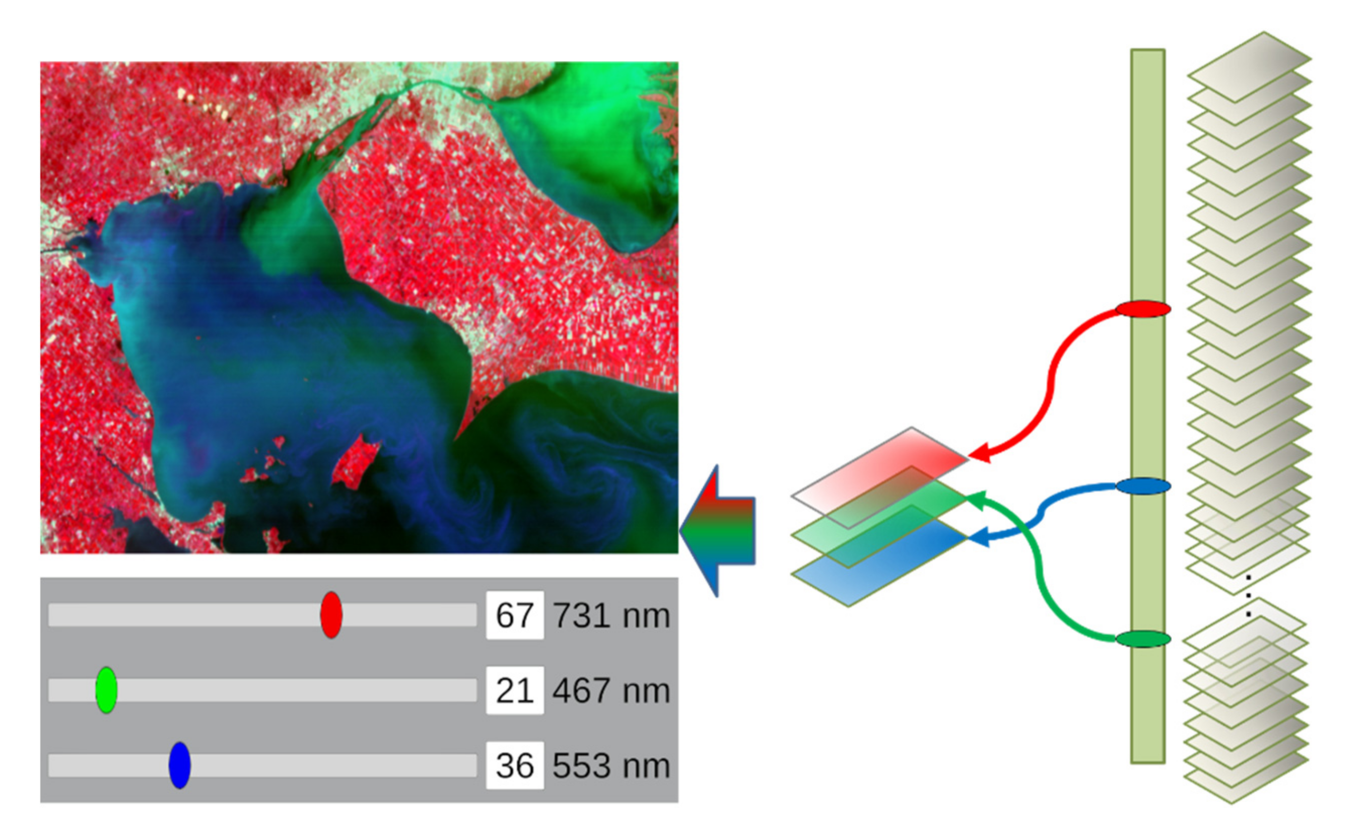
Common visualization methods for hyperspectral data include the simple combination of three greyscale images of spectral bands into RGB false color images, as well as the image cube, in which one row and one column on the borders of a hyperspectral image are visualized using a rainbow color scale, where the red end symbolized a high reflection in the respective spectral band, and the blue/violet end symbolizes low reflection. Both are complex to use and interpret in geographic information systems (GIS), and thus need to be simplified for the app, both in terms of user experience and computation power. In addition, their use should be interactive, instantaneous, and tangible for the students to be able to play with the data.

Several restrictions have to be considered:

• The lesson, consisting of a work sheet and app, is supposed to encourage teachers and students to explore RS and hyperspectral data. This would be futile if the data or software were behind paywalls for the target group, so they have to be freely available.
• Teachers cannot be expected to have deep knowledge about the data, the processing, or the specific incident and region analyzed in the worksheet and app, nor can they be expected to understand the app intuitively, even if it is designed that way. They also have limited time to prepare for their many lessons. Hence, every step has to be explained, sample solutions and background information given, so the teacher is perfectly prepared without any additional research.
• As teachers already have very little time to cover the curriculas’ demands and very rarely time to do anything outside these curricula, the worksheet and app must fit into those curricula.
• IT infrastructure is still lacking in German schools including Wi-Fi. Neither teachers nor students can rely on streaming while at school. Every part of the app has to be downloadable at home and small in size to be ready when the lesson begins.

The app and worksheet resulting from these requirements were evaluated with two advanced geography courses, with 18 students each, using a closed yes/no questionnaire about previous knowledge before the lesson and about understanding of the individual parts at the end of the lesson. These two courses were chosen because the teacher regularly uses satellite imagery in her lessons and works closely with the project this study is a part of (KEPLER ISS). A larger sample size was not possible due to the COVID-19 regulations in Europe having started the week after the evaluation.

This paper will start with the technical side, explaining the RS data and the methods applied to them (Section 2.1), and will then describe the development of the AR app using the processed data (Section 2.2). The educational concept is then presented (Section 2.3), followed by a description of the worksheet tasks, in combination with the app functions (Section 2.4) and teacher materials (Section 2.5). Finally, an evaluation of the app, performed in a real class environment, is provided (Section 2.6).

2. Materials and Methods

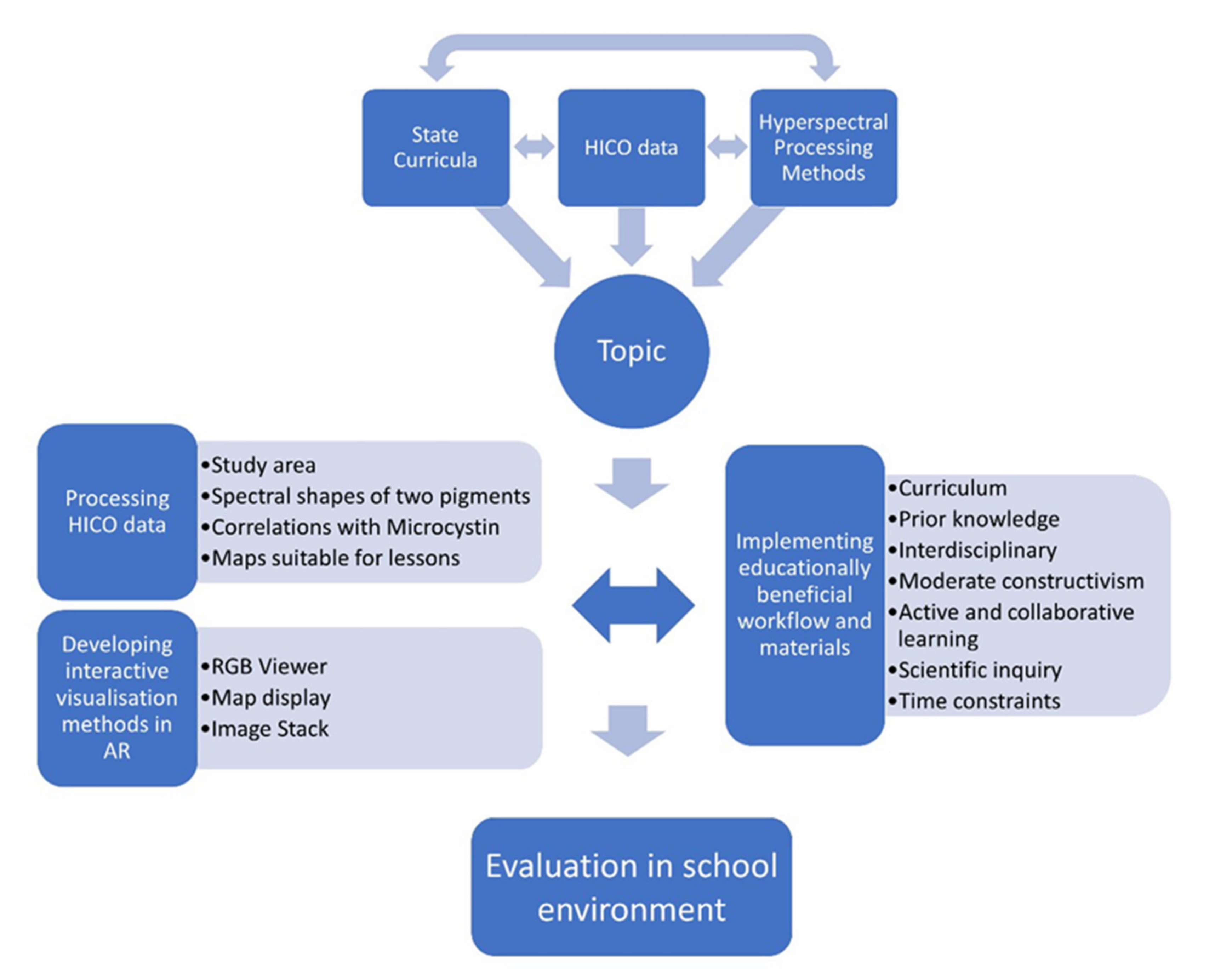
All three aspects of RS methodology, AR development, and an educationally sound workflow were executed simultaneously, as shown in Figure 1. Hence, the topic was chosen as a combination of (1) available data from the chosen sensor, (2) processing methods understandable for high school students, (3) high relevance for at least a few states curricula. Any unexpected changes to one of the three aspects were reassessed for the other two at all times. Ultimately, the published app and workflow were evaluated with students in a real school lesson environment.

The Hyperspectral Imager for the Coastal Ocean (HICO, Arlington County, VA, USA) was a hyperspectral imaging sensor aboard the International Space Station (ISS) that captured freely available data between September 2009 and September 2014. It was chosen as a basis for the data since the project this work is part of, KEPLER ISS, aims to include the astronauts’ view on Earth with a variety of ISS-borne imaging sensors to be used in STEM education [19,21], as this particular view has great potential to excite students for STEM [13]. At the time of development (2018–2019), HICO was the only ISS-borne hyperspectral imager and one of only two hyperspectral imagers with freely available data, the other being Hyperion. While Hyperion was in orbit for a much longer time (2000–2017) and has a better resolution (10–30 m) than HICO, its swath width is also much smaller at 7.7 km, further limiting potential applications for educational material.

One image was taken per ISS orbit, which takes 90 min each. Each scene consists of 128 bands between 353 nm and 1080 nm wavelength, however, only 87 between 400 and 900 nm are usable (see Figure 2), as the ones above and below those wavelengths contain a lot of visual noise, i.e., stripes and blur. Each image is 2000 by 512 pixels in size. The images’ spatial resolution varied around 90 m due to the orbit constellation of the ISS [22]. Over 10,000 scenes were taken. However, many analyzed rock formations, and only very few were suitable for any topic that could be covered in lessons. The authors searched specifically for algal blooms in Europe, since the materials are to be used primarily by German schools, but no image covered a sufficiently visible bloom. In the end, the algal bloom in Lake Erie was determined to be the best topic to create a lesson from under the given requirements. HICO data can be downloaded for free at the NASA Ocean Color portal and processed with the free ESA Sentinel Applications Toolbox.

2.1. Remote Sensing Data and Methods: Preparing Hyperspectral Imagery for Use in an AR Lesson

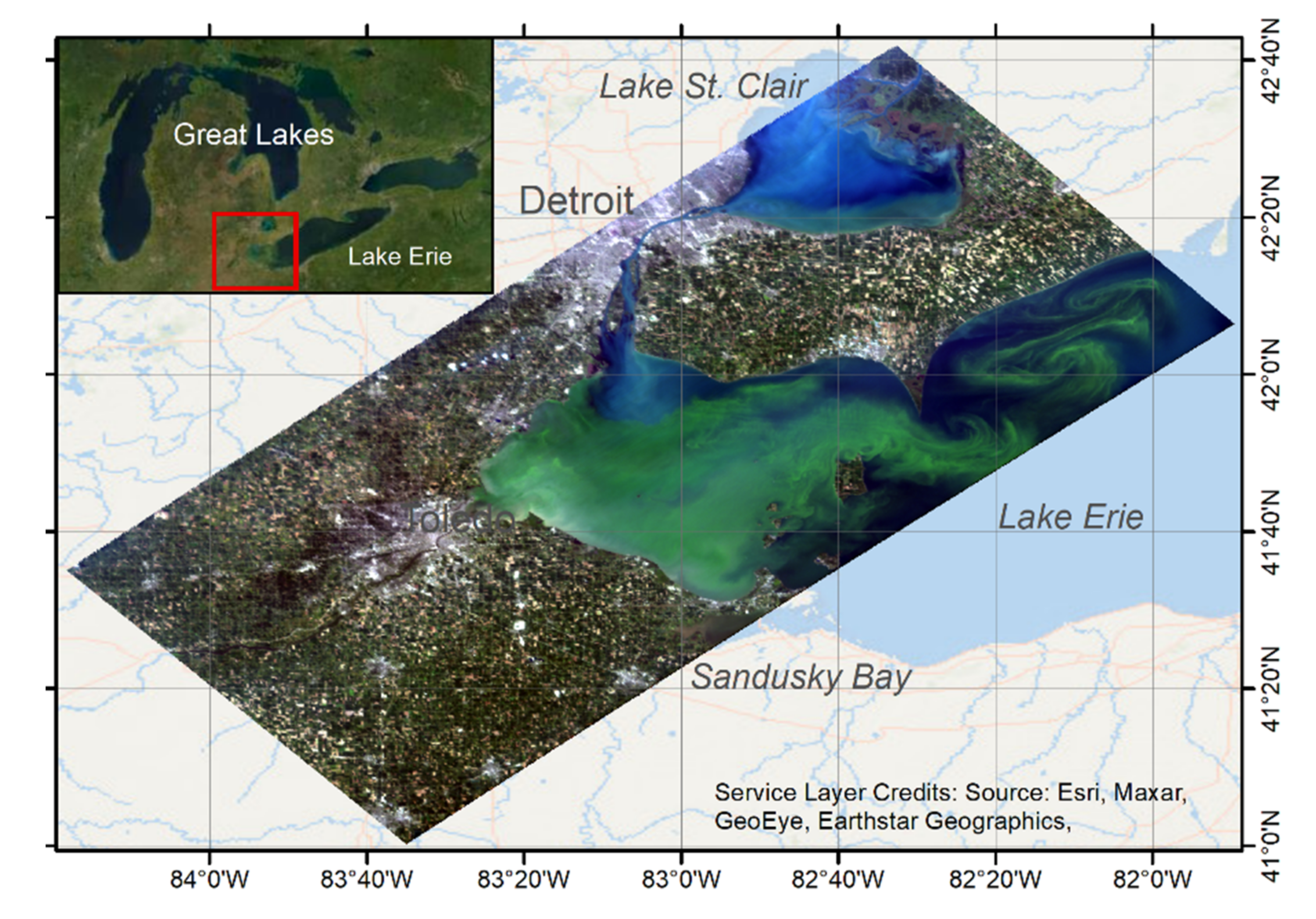
Lake Erie is the smallest and shallowest of the Great Lakes and thus warms quickly in spring and summer. The shallowest part, with an average depth of 7.4 m, is the western basin, where the focus of this study lies. It is connected to the upper Great Lakes through the Detroit River and the much smaller Lake St. Clair (see Figure 3). This accounts for 80% of Lake Erie’s total inflow, with only 9% coming from other tributaries and 11% from precipitation. Retention time in the lake is about 2.6 years before the water leaves the Lake, through the Niagara river at the eastern end [23].

The Lake Erie watershed is inhabited by 12 million people and is largely agricultural with several industrial centers, including the city of Detroit. Compared to the other Great Lakes, it has the highest stress from effluent, but also sediment loading due to the local geology and land use [23]. The increasing phosphorus load from agriculture provides nutrients for algae growth and certain weather conditions, that are expected to occur more often in the future due to climate change, can lead to extreme blooms of harmful cyanobacteria in the lake [24]. Since 2008, the yearly algal bloom in Lake Erie exceeded the desired maximum in all but one year, with 2011 and 2015 standing out due to their extreme algal bloom events [25]. Water from Lake Erie serves as drinking water for about 11 million people nearby [23].

2.1.1. Spectral Shape Algorithm to Distinguish Harmful from Harmless Algae

Data was extracted from an HICO scene from 3 September 2011 displaying an algal bloom in the western basin of Lake Erie and the adjacent Lake St. Clair. Remotely sensed chlorophyll a from MERIS data was used by the NOAA for their weekly information bulletin during the bloom. However, chlorophyll a concentration does not translate well into toxin concentrations from cyanobacteria as it is an indicator for all kinds of phytoplankton [26]. Ref. [27] chose phycocyanin as a cyanobacteria indicator. It can be distinguished from chlorophyll a using spectral shapes (SS), or second derivatives, in the spectral signatures of both pigments, according to the equation

$$SS\left(\lambda \right)=\mathrm{R}\left(\lambda \right)-\mathrm{R}\left({\lambda }_{-}\right)+\left(\mathrm{R}\left({\lambda }_{-}\right)-\mathrm{R}\left({\lambda }_{+}\right)\right)\ast \frac{\left(\lambda -{\lambda }_{-}\right)}{\left({\lambda }_{+}-{\lambda }_{-}\right)}$$

(1)

in which R is the reflectance or radiance, $\lambda$ is the band with the central dip, ${\lambda }_{-}$ and ${\lambda }_{+}$ the bands with the adjacent peaks with shorter and larger wavelengths, respectively. This SS was used as a chlorophyll index (CI) by [28] and has been used and adapted widely in the detection of algae [24,29,30]. Due to the second derivative, top-of-atmosphere data works similarly well as atmospherically corrected data [31], hence no atmospheric correction was performed. While [27] applied this to MODIS bands, which are not optimally spread out to cover the dips and peaks of the two pigments, HICO has the advantage of back-to-back bands, allowing adjustment of the equation much more exactly to the actual SS. The local absorption maximum of phycocyanin is found at 620 nm, coinciding with MERIS band 6 [26,27], whereas spectral signatures show the local absorption maximum is closer to 630–640 nm [27,30,32] and [26], who used band ratios instead of SS, determined the best ratios at 630–640 nm to 650–660 nm. Neither the two pigments, nor the water they are dissolved in, absorbs strongly around 709 nm [27].

Study [30] showed that the SS in (1) can be applied to HICO data but did not specify which bands were used. The wavelengths given could be used to determine HICO bands for the detection of phycocyanin, while the wavelengths given in [27] were used for the detection of chlorophyll a. The wavelengths were adjusted to the available HICO bands in relation to the absorption minima and maxima of the two pigments, resulting in the wavelength combinations in

Table 1. HICO bands chosen for the detection of chlorophyll a and phycocyanin through the spectral shape. (Data source: https://oceancolor.gsfc.nasa.gov/hico/instrument/dataset-characteristics/, accessed on 1 December 2021).

	Chlorophyll a	Phycocyanin
${\lambda }_{-}$	650.4 nm	558.7 nm
$\lambda$	679.0 nm	638.9 nm
${\lambda }_{+}$	707.7 nm	650.4 nm

.

In the 2011 Lake Erie bloom, the phytoplankton consisted almost entirely of potentially toxic Microcystis in August and was replaced by the also potentially toxic Anabaena after Microcystis had depleted the bioavailable nitrogen in the Lake [24]. Both species are cyanobacteria containing the phycocyanin pigment and thus show the characteristic local absorption maximum at around 638 nm [33,34]; thus, no change to the selected band was necessary. Due to the high variability in the relation between detected phycocyanin and the exact species composition in the 2014 data [27], no correlation between the concentration of the detected pigments and the occurrence of certain algae was determined. The maximum CI detected in the HICO scene corresponded well with the annual CI from MODIS composites in [35], but, due to the high interannual variability, also iterated in [27], no correlation from that data was determined. For the students, the CI values would make no sense; thus, these values have to be converted into something more useful, such as pigment concentrations.

2.1.2. Correlation of Pigment with Toxin Concentrations

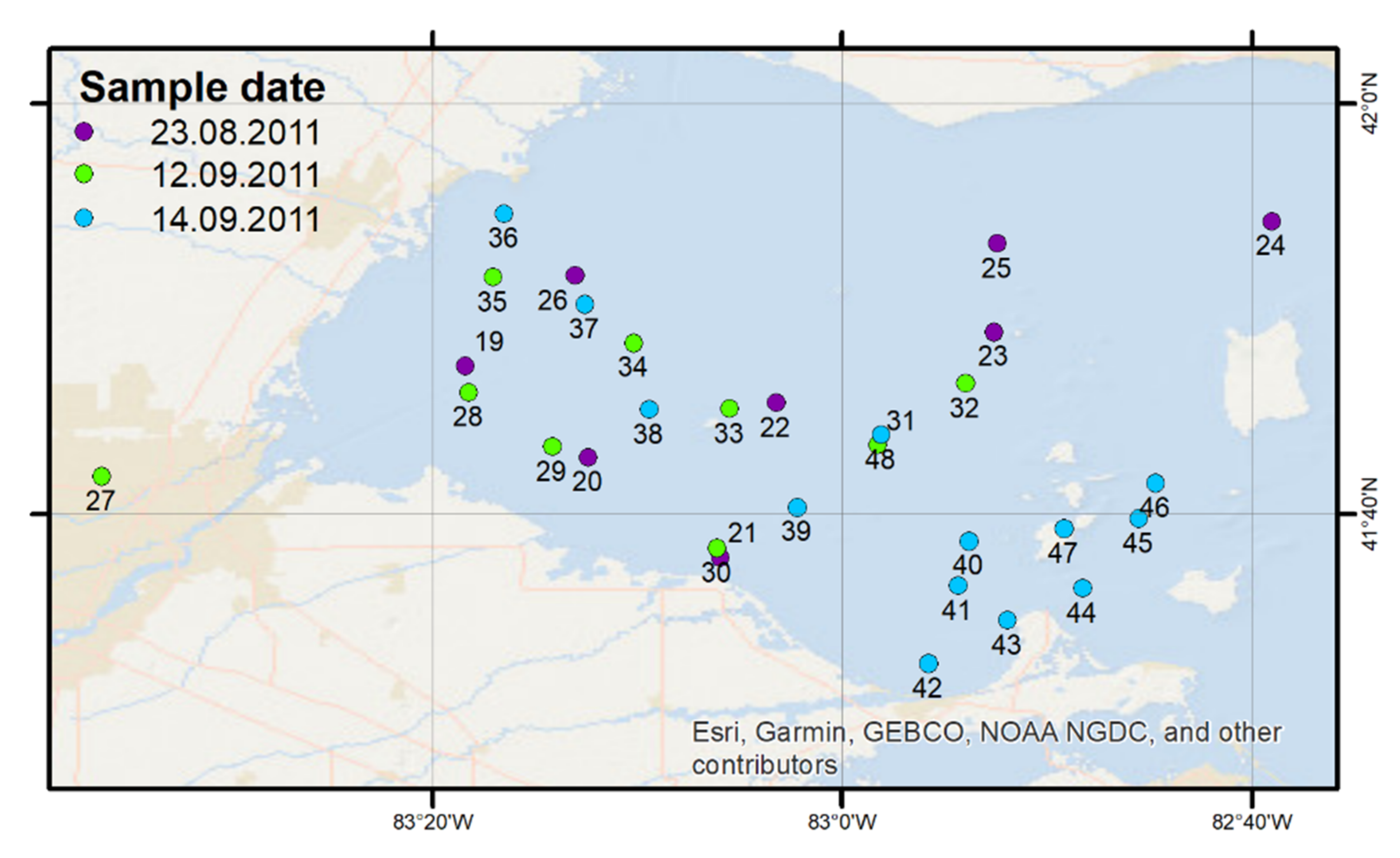
Biological data was provided by the Cooperative Institute for Great Lakes Research (CIGLR), who performed an extensive bloom survey in 2011. The in situ samples taken closest to the HICO acquisition date were taken on 23 August, 12, and 14 September 2011 (see Figure 4). The values show a high spatial and temporal variability, with extracted chlorophyll a ranging from 18.88 µg/L to 109.20 µg/L (both 23 August) with no data for 14 September and extracted phycocyanin ranging from 0.67 µg/L to 10,855.30 µg/L (both 14 September). The latter was an extreme outlier sampled in the northern bay of South Bass Island that is rather shallow and used as a marina. Hence, it was not included in the following considerations. The data of 29 individual measurements from the above for phycocyanin and microcystin from these three days could be used; however, there were no chlorophyll measurements for 14 September, reducing the total number of measurements for this pigment to 17. This was not enough for a scientific analysis; however, since the goal was “only” to demonstrate the use of hyperspectral imagery to school and college students, it was viewed as sufficient.

Between measurements, water in the lake moved significantly. A total of 11 days passed between the first in situ measurement and the acquisition of the HICO data, and then another 9 days until the next measurements. As [36] demonstrated for the algal blooms in Lake Erie from 2008 to 2010, the concentration distributions can vary drastically in a short span of time, and [24] supplement data suggests medium circulation conditions. In situ measurements cannot, therefore, be correlated to the pixel values in the same, or even close, positions. The modeling necessary to produce accurate results is beyond the scope of this work, especially considering its overall goal.

Nonetheless, this data is valuable to relate the chlorophyll a and phycocyanin indices measured from the HICO data. The next highest phycocyanin value after the extreme outlier was 1327.05µg/L that was sampled in between the western islands and was much closer in value to the next two highest sampled values and their locations. It was also the closest to the highest values of phycocyanin detected in the HICO images from a few days before.

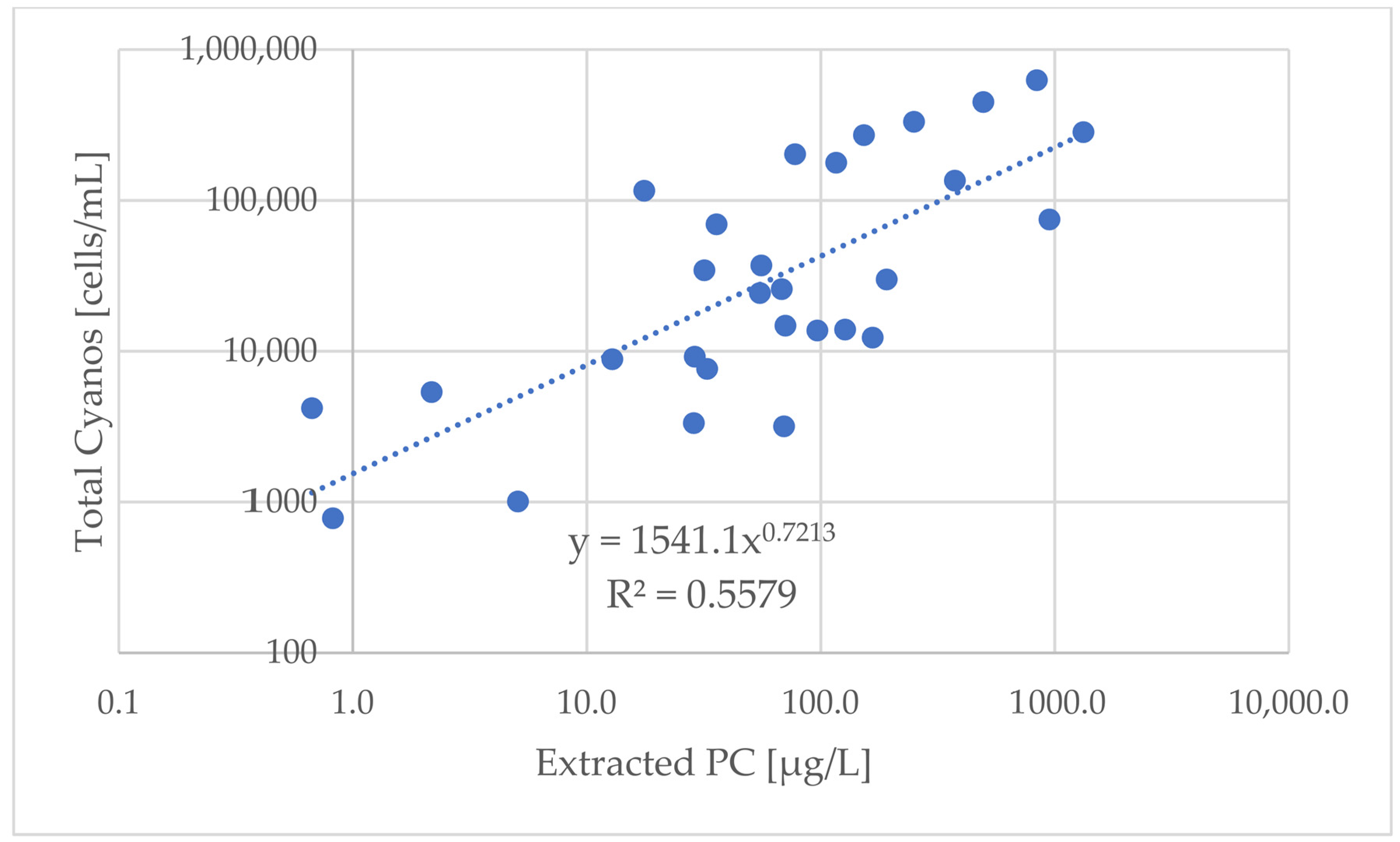
While [27] states that twice the concentration of phycocyanin is needed for an equivalent response to a given concentration of chlorophyll a, this is only true when using the same spectral bands. Assuming the maximum phycocyanin concentration from the satellite imagery to be in the same range as the maximum concentration from the in situ samples was the closest approximation possible without extensive modeling; thus, the maximum value of 67 in the phycocyanin map was assumed to be equal to the maximum value of 1327.05 µg/L from the in situ measurements. For the minimal value of 30 in the phycocyanin map, the total cyanobacteria cell count had to be considered. A response in the spectral data was not expected below a cell count of 10⁴ mL⁻¹ in the MERIS data [27], however, in the biological data, there was large variability between the phycocyanin and cyanobacteria cell counts (see Figure 5). Using a regression curve, the threshold of 10⁴ cells/L was met at roughly 10 µg/L phycocyanin. Hence, this was used as the minimum value.

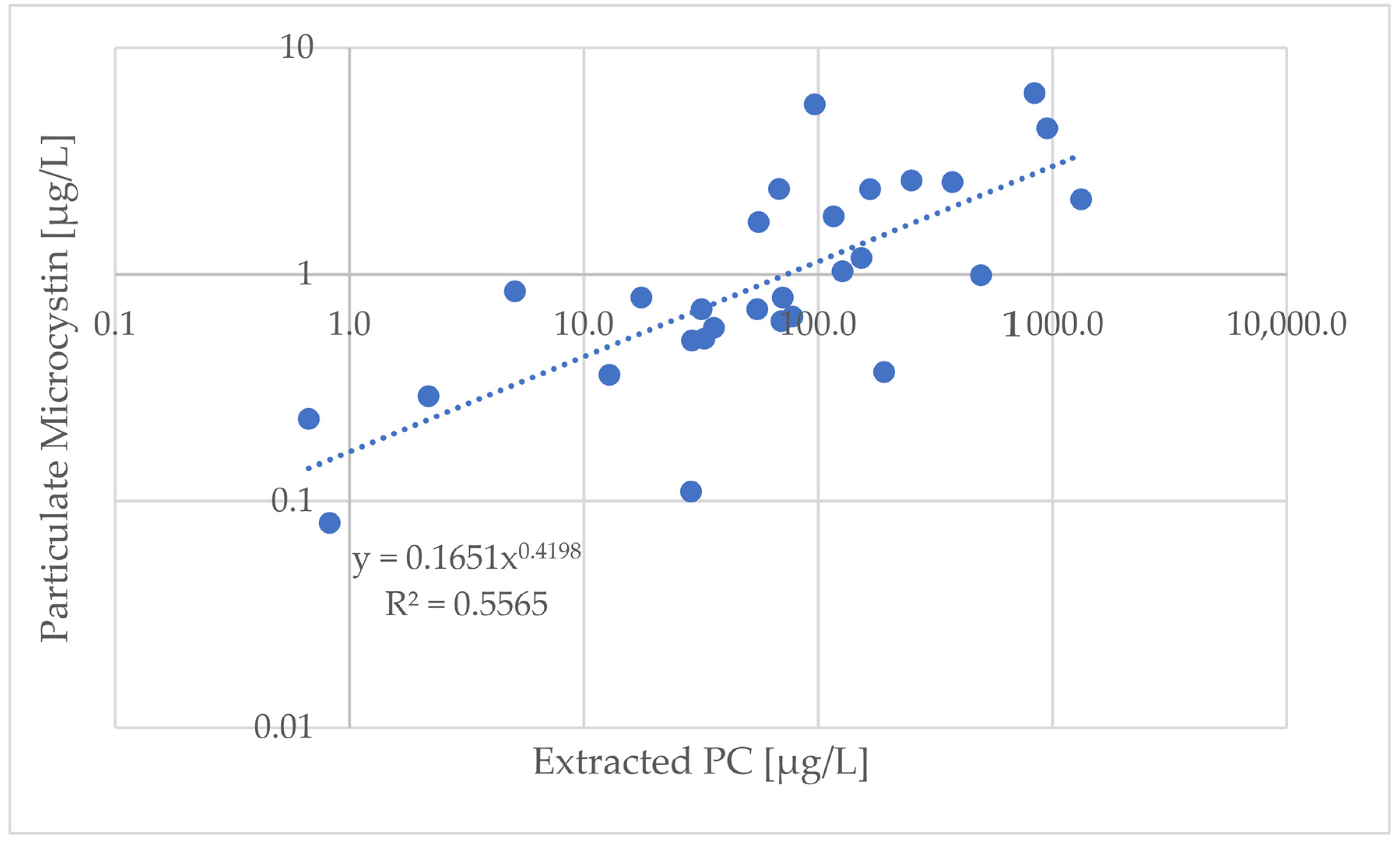
As for the 2013/2014 data in [27], a double logarithmic relation between phycocyanin and microcystin can be deduced from the 2011 biological data (see Figure 6).

Furthermore, the relationship between the CI and chlorophyll a was more or less linear [37] and, since there are no similar studies for phycocyanin yet, it was assumed to be linear here as well. The resulting values can be seen in

Table 2. Phycocyanin index derived from HICO image, correlated with phycocyanin in situ measurements, and correlated with microcystin concentration.

Phycocyanin Index	Phycocyanin [µg/L]	Microcystin [µg/L]
67	1327.07	3.38
30	10.05	0.43

.

For chlorophyll a, the lowest value detectable by the CI was between 10 and 20 µg/L [27]. The minimum CI value was 4, the maximum was 17. There were no chlorophyll measurements on the day or in the area with the highest and lowest phycocyanin measurements. The highest CI values for chlorophyll were in a completely different area than the highest measurements, while the measurements roughly in the same area as the highest CI values were moderate with respect to the overall highest measurements. On the other hand, the highest CI values were spatially very limited in an area with moderate values. This was the only data available and, despite the small sample size of chlorophyll a (17 samples), it was used in the same way as the phycocyanin data (see

Table 3. Chlorophyll Index derived from HICO image, correlated with phycocyanin in situ measurements and correlated with microcystin concentration.

Chlorophyll Index	Chlorophyll Conc. [µg/L]	Microcystin [µg/L]
17	109.2001	4.46
4	18.88	0.38

).

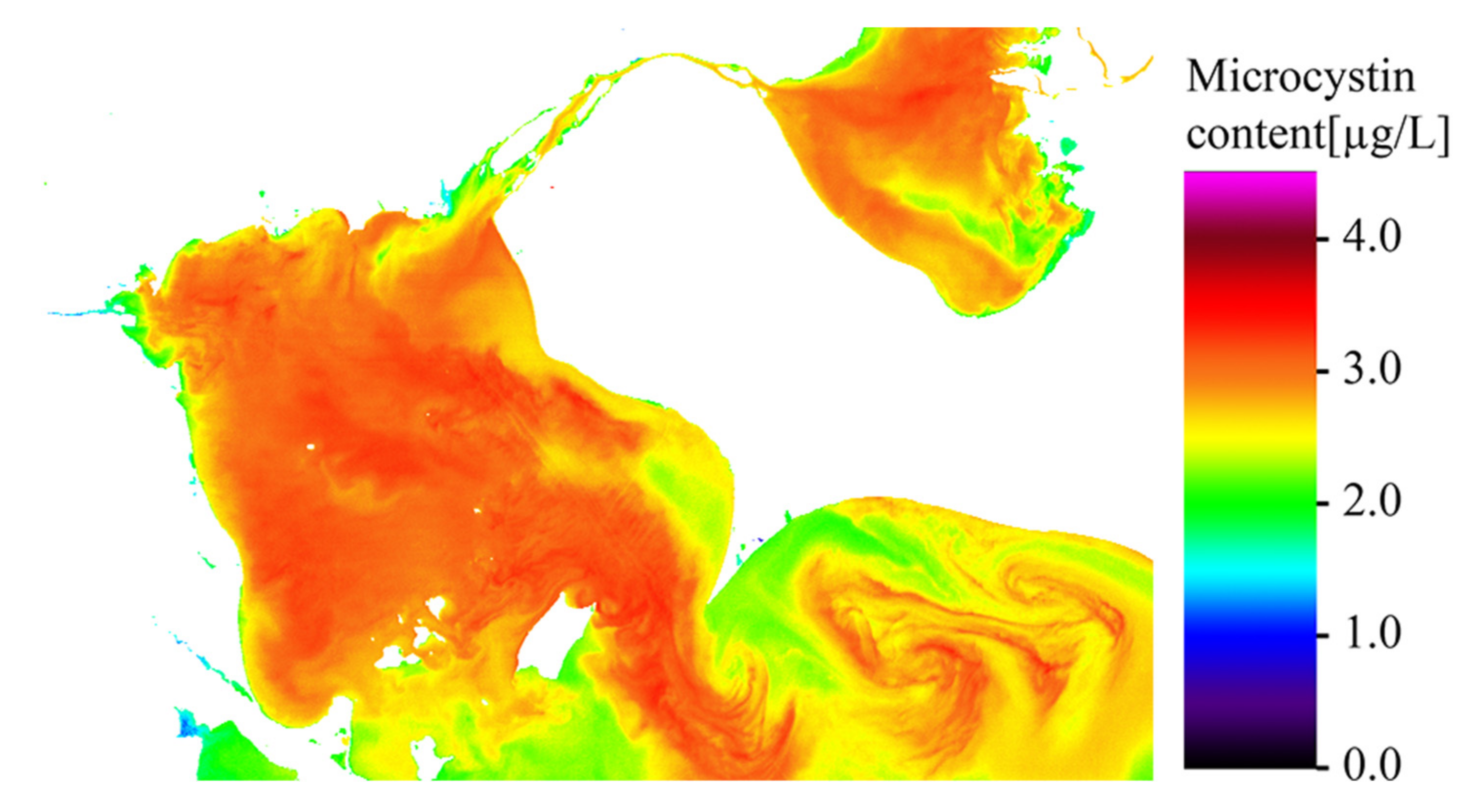
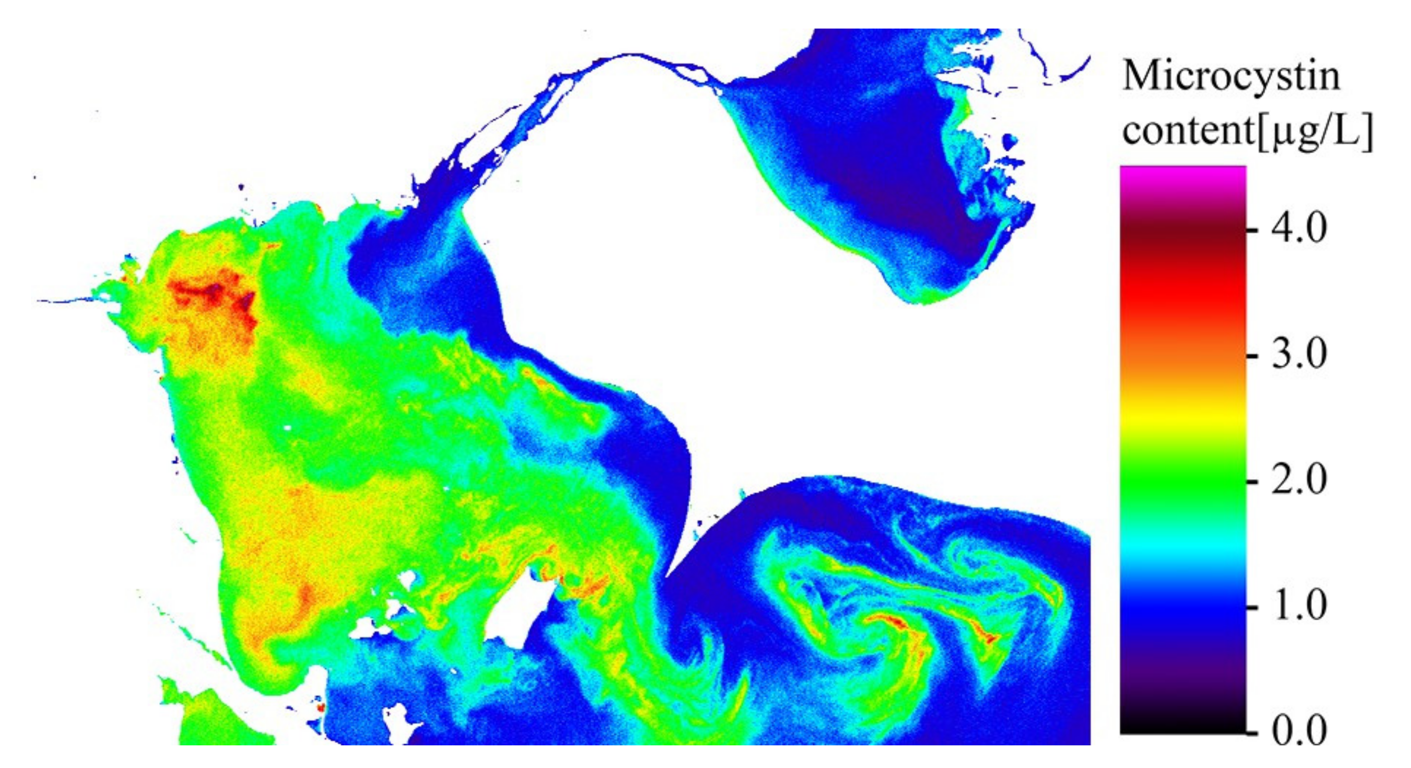
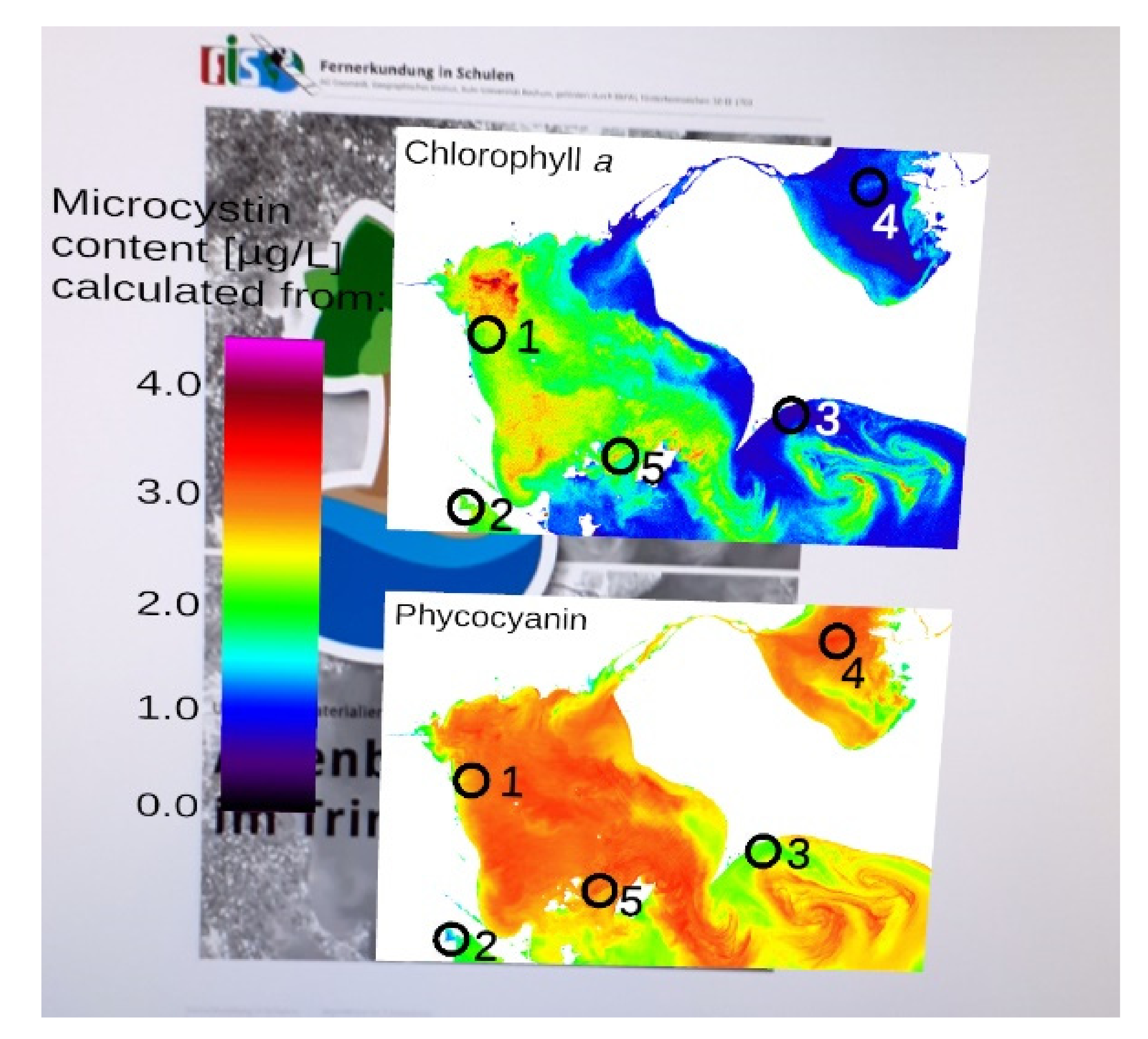
The correlation of the pigments with toxins resulted in the maps in Figure 7 and Figure 8:

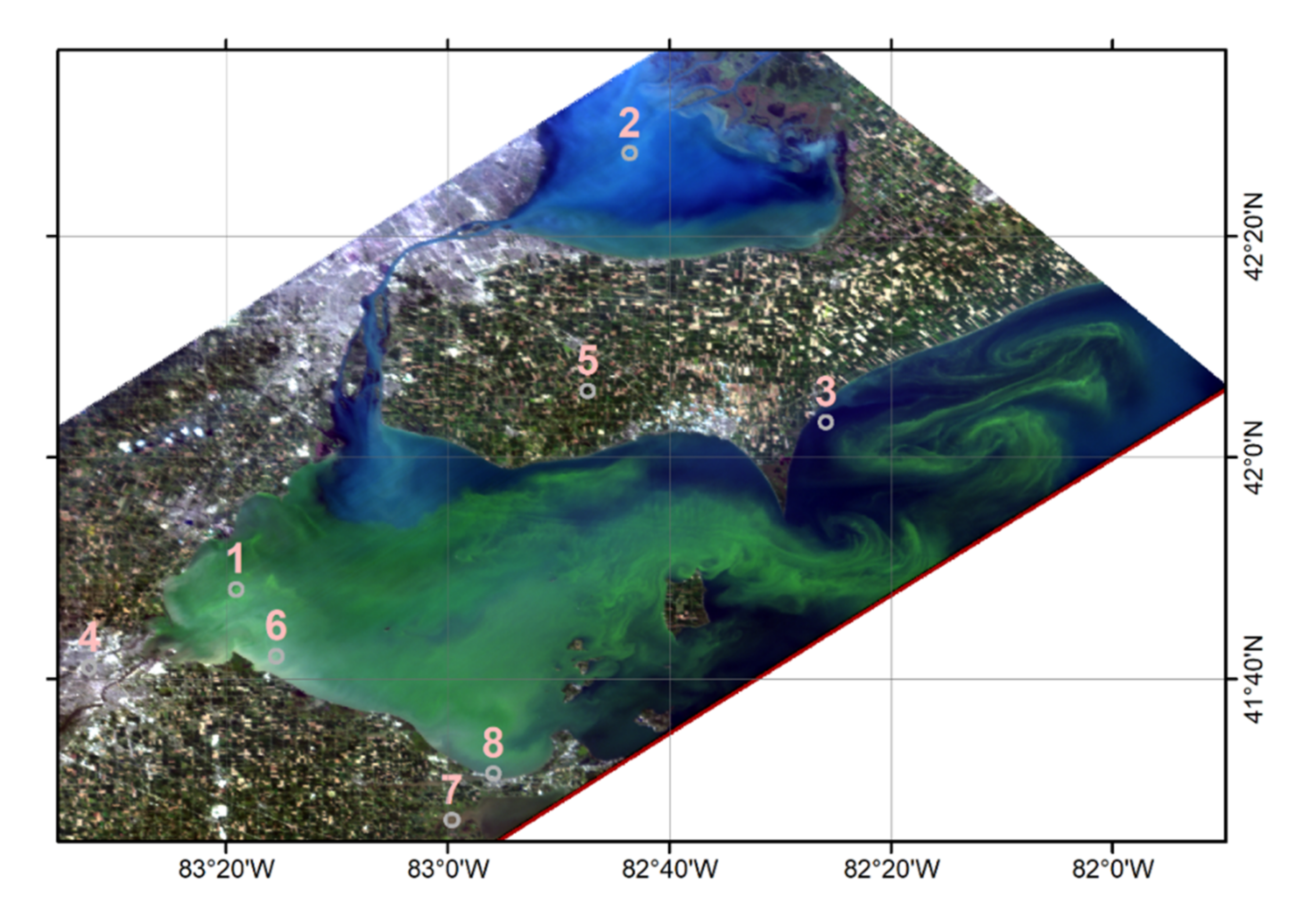
In addition, 8 pixels were chosen to extract spectral signatures from display in the app representing certain types of surfaces or certain places. The points chosen are shown in Figure 9.

2.2. Application Implementation

The AR app is part of an extendable unified AR platform in the project Columbus Eye/KEPLER ISS [13,19] and was developed in Unity 5.6 with the Vuforia extension 6.2 by the main author of this study.

The app featured in this paper consists of four main parts. The app starts with a video of algal blooms around the world, as seen from the ISS, to introduce the AR functionality with a simple interaction—pressing a play button. It is included as a simple video overlay on an image target, using a video cut from scenes taken by NASA’s high definition Earth viewing (HDEV) cameras [38], showing a variety of marine algal blooms. The second element is a UI that displays an RGB viewer of the HICO scene with spectral signatures (RGB Viewer). The third is a collection of maps: A Landsat 5 image taken shortly before (3 September 2011, 15:59 GMT) as the HICO image (3 September 2011, 17:34 UTC) for comparison with a higher spatial resolution. In the Landsat image, boat wakes and small differences in surface algae concentration are visible, and the two maps of microcystin derived from chlorophyll a and phycocyanin, respectively. The fourth and final element is an image stack where all images from the scene are stacked on top of each other.

2.2.1. RGB Viewer

The UI displays the HICO scenes as an interchangeable RGB image. Three sliders in the lower third of the display define which bands the RGB image consists of and there is a display for spectral signatures at the top. The image is not oriented, as this would lead to large white corners (compare Figure 9 with Figure 10). Instead, the students are supposed to find out the cardinal directions in comparison with one of the marker images (Figure 13, p4) that is oriented properly.

The scene was cropped in order to focus on the lake and resampled to compensate for the non-quadratic ground sampling distance, reducing the image size to 491*725 pixels. Each of the 87 bands used was stored in PNG format with 8-bit grayscale. This reduces the total file size of the scene from 591 MB to 18 MB. The band images are not “read/write” enabled as this would double the required data storage and increase the required computing power. Due to the AR camera functions, depending on the smartphone model, there is very little computing power left for the remote sensing data.

As the RGB image from the individual bands cannot be computed without “read/write” enabled ([13]), another solution had to be found. Unity 5.6 provides the developer with a range of different shaders that are designed for 3D-environment development, which is ideal for game worlds. Shaders define the way surfaces are rendered. This can include how they are affected by light sources, how colors are displayed, metallic or skin effects, etc. However, there is no shader available that would do the same as a calculated RGB image from grayscale bands in regular GIS (i.e., multiply one grayscale band each with red, green, and blue and add them together). While the documentation on the high-level shading language (HLSL) that Unity utilizes is rather limited, a shader equal to the required task could be compiled from community resources. As visualized in Figure 10, this shader simply reads the pixel grayscale value at any given coordinate of the required band and multiplies it with the color and alpha or transparency values defined in the 3D object that holds the band. This object is one of three planes colored in blue: no transparency, green: 67% transparency and red: 84% transparency, stacked right on top of each other. The transparency values were defined by testing. This method works instantaneously, and the user can slide through the bands in real time using the three color sliders at the bottom of the UI. Alternatively, the band number can be typed in, making the band definition easier on smaller displays, where the difference between two neighboring bands on the display may be too small for human fingers to select.

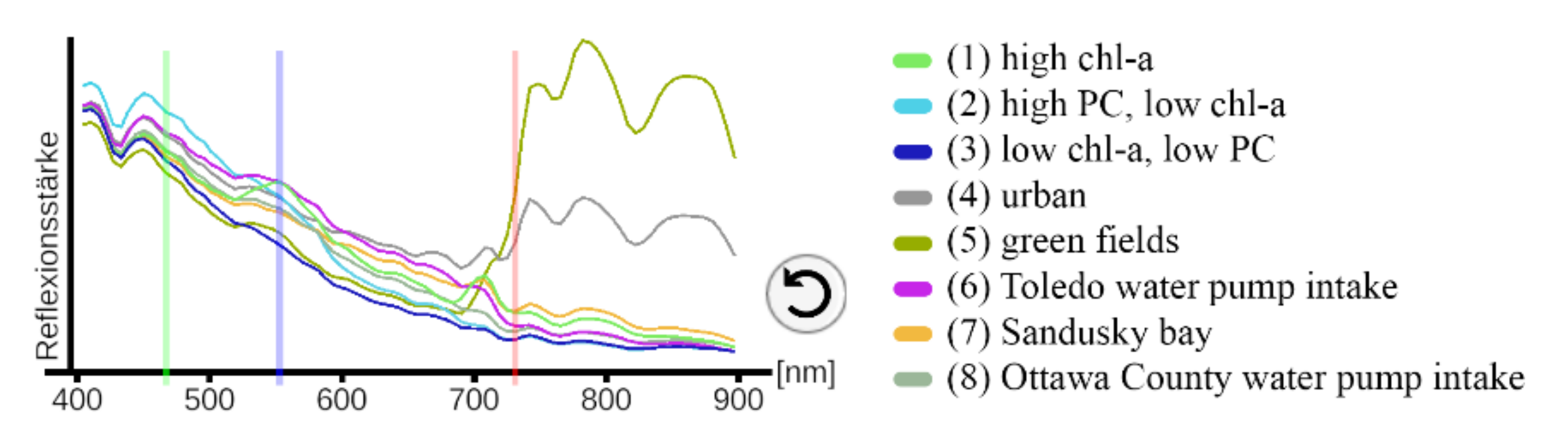
Spectral signatures are to be displayed as well, emphasizing the use of hyperspectral data for the students. As the images are not read/write enabled, this data cannot be read in real time from the images and has to be prepared. Eight signatures were extracted as examples for certain surfaces (cf. Section 2.2.2). These signatures can be made visible by hitting invisible buttons on the image. The lines are drawn with the “LineRenderer” asset and a script filling each line with the values from the spectral signatures. Colored bars represent the bands chosen in the RGB viewer and help the students to connect between spectral features and coloring, as seen in Figure 11.

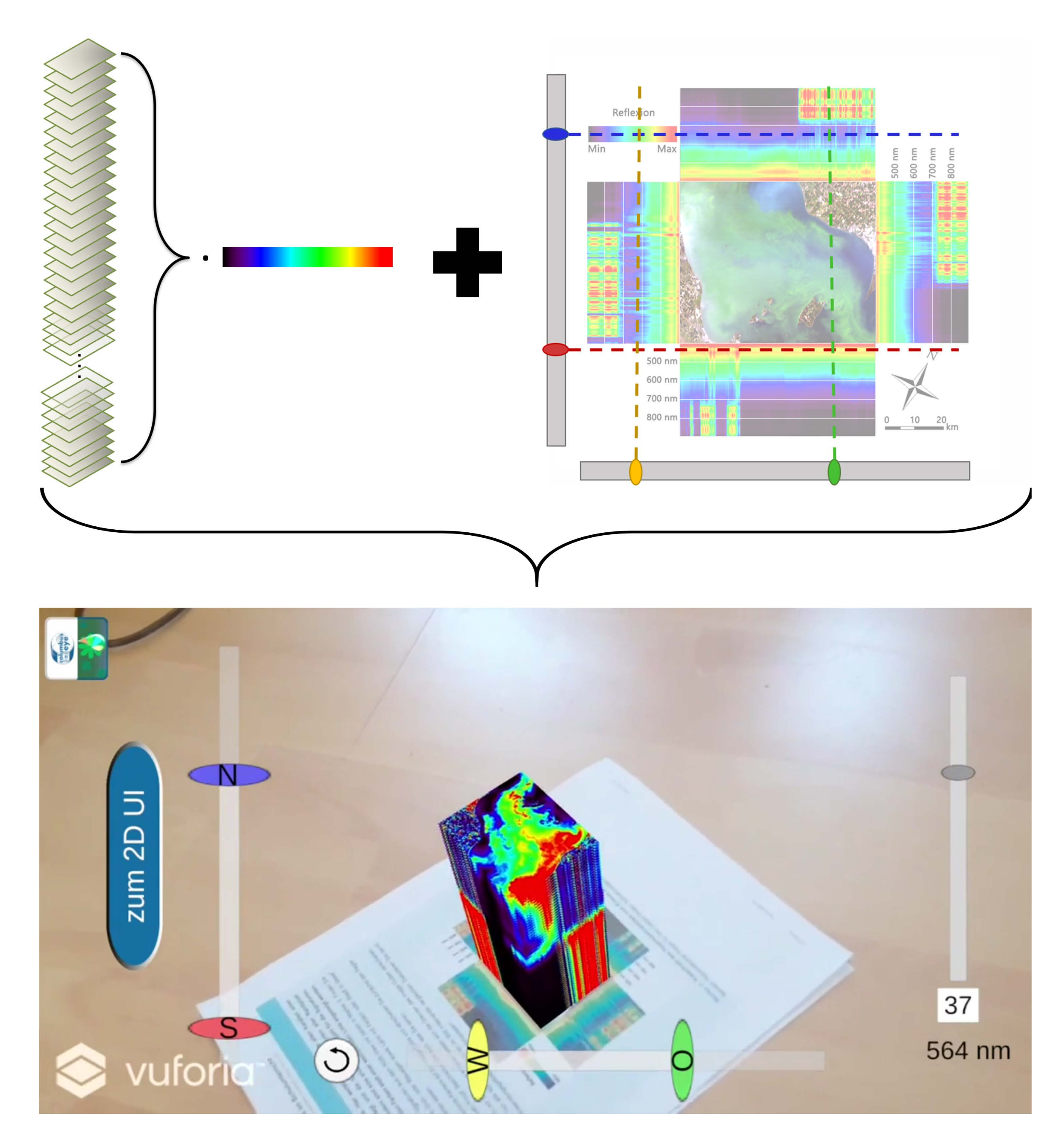
2.2.2. Image Stack

The image stack was developed based on the so-called image cube, a visualization method for hyperspectral data that displays the spectrum of all edge pixels of a given image using a color bar. In, e.g., ENVI, acquiring one image cube is complicated and requires many steps, but only gives the profiles of one row and one line of pixels. In the EnMAP Toolbox, one slice of each axis of the cube can be picked with enough knowledge of the program. The image stack in this app is meant to give the user access to all possible profiles of the hyperspectral image in a very easy way, with little background knowledge required. It is displayed on top of a static worksheet image; a true color RGB image subset of the original image that has all edge pixels’ profiles displayed in the style of the ENVI image cube serves as a marker. A legend, north arrow and some annotated lines help both the users to understand what they see and Vuforia to recognize the image due to additional, detectable edges [13].

In Unity, the image target has a script attached that loads the individual band images and creates quad objects to store them. A quad is a primitive type of game object that only has four vertices in the four corners, as opposed to a plane, cylinder, etc., which have many vertices. While this makes little difference for a single quad versus plane, using 87 quads will significantly reduce computing power in comparison.

The quads are not created until the required marker image is detected. Then, each quad is created according to the specifics (e.g., size, scale, rotation, position plus a few pixels upward) of an inactive example quad attached to the image target in Unity. Each quad receives a renderer with a custom shader and a script to move the quad out of sight.

The shader has to fulfil two functions (see Figure 12): color each grayscale image in the color scale of an image cube and cut off the sides of all the quads so the user can see inside the image stack. Again, no Unity shader can achieve this, therefore a custom shader was created. This shader utilizes an image with the fixed color bar that is loaded into Unity and replaces the grayscale value from each pixel of the band image with the color at the according horizontal segment of the color bar. In addition, it is fed four vectors defining the borders: values from 0 to 1 for North/South and East/West. Everything outside these borders is clipped, meaning the pixels are not rendered. The shader was compiled from freely available open community resources.

The default borders are set to the same values as the image in the marker image. They are accessed by a script attached to the container for two double sliders in the image stack’s UI. Each slider handle (N/S, E/W) is prevented from going past the complementing one and can be one of as many values as the image width and height, respectively, making the minimum displayed profile that of just one pixel. A button to reset the borders to the marker image borders is included.

The quads can be moved out of the view of the smartphone camera but are not destroyed or disabled due to the high number of errors that occurred using these methods. Another slider in the image stack’s UI defines which band is displayed at the top, with all the higher band numbers being displayed below, while lower band numbers are moved out of the camera view.

2.3. Educational Concept

Due to the combination of physics (characteristics of the electromagnetic spectrum), biology (cyanobacteria, green algae, nutrient cycles), and geography (RS, landforms, agriculture), the materials are highly interdisciplinary and thus have to be contextual, instead of fitting tightly into one subject’s structure [39], while still fitting into one of the regular subjects. Geography is the subject that brings other STEM subjects together to apply them to the real world and is thus chosen as the main subject to focus on. In applying theoretical and practical knowledge from the past few years of their regular education, students learn that studying these, often considered boring, subjects can lead into interesting careers. However, at this point, not all of the prior knowledge and competencies from all three disciplines can be expected from every student. Thus, before the lessons start, students are to prepare themselves in a flipped classroom approach [40]. The learning materials are based on a moderate constructivist approach [41] with active and collaborative learning [40]. The instructions lead to scientific inquiry, encouraging the students to think actively and draw their own conclusions from their prior and newly acquired knowledge [42], which has been proven the most effective approach to increase conceptual understanding [43]. The ultimate goal of the learning material is to use STEM knowledge with complex RS data and methods to discuss problems and solutions in order to make spatial decisions. At the same time, it has to be simplified enough for students to be understandable and solvable within the 90 min a typical double lesson takes. Finding the balance between realistic and simple is one of the most complicated tasks in this endeavor. In addition, the smartphones have to be used productively, demonstrating for the students that computers of any size can be used for more than social media, but also as tools to visualize scientific data in tangible ways.

In order to understand how hyperspectral data work, deeper knowledge of the electromagnetic spectrum is required, which should have been learned in physics lessons in the previous years of school. To learn how hyperspectral data is applied to the detection of algae, the students need to know the basics of how algae live and what chlorophyll is and does, which should have been covered in prior biology lessons. On top of that, the students must have learned about the broader topic of environmental problems from agricultural practices before, so as to present the topic in the right context. Due to the federal structure of education in Germany, any of these topics are covered in different years on different levels per federal state, ranging from grade 7 to grade 10 [44,45,46]. Even then, not all students are at the same level of understanding due to differences between individual schools. Hence, the very complex topic chosen for this study is implemented on a level expected from students in the final three years of high school.

Students of this age are expected to display certain hard and soft skills in the subject of geography, but also from other related subjects, as knowledge gathered from other subjects is compiled and applied in geography. These performance requirements are defined in detail in the curricula of North Rhine–Westphalia [47], which are the basis for this app and worksheet. The main topic the app and worksheet fit in is “habitats and their natural and anthropogenic endangerment”. The required soft skills include, but are not limited to, human-environment interactions, reading thematic maps, technical methodologies, analysis and interpretation of geographic information, use of technical terms, good judgement regarding land use and its consequences from a variety of perspectives, as well as using all of these autonomously and presenting their results in a professional manner. All of these are propaedeutic skills that prepare the students for their academic studies in many fields of science. The workflow was thus created considering these soft skills.

In other German states, the app and worksheet fit into similar overarching topics of anthropogenic influences on natural resources, e.g., “Water as the basis of life” in grade 11 in Bavaria, that includes anthropogenic influences on the water supply [45], “Use of resources” in grades 9/10 in Berlin and Brandenburg [46], and “Sustainable use of resources” in grades 12/13 in Hesse [48].

The holistic framework for the evaluation of learning materials by [49] takes many of these skills into consideration as well, albeit more abstractly for use in different subjects, and is thus both a guide for the development of the worksheet and app and used in their evaluation.

2.4. Workflow of App and Worksheet

The worksheet and the app are designed to work together—neither makes sense without the other. Hence, the workflow is described as one.

For repetition, or catching up, about the characteristics of electromagnetic waves, two learning videos are to be watched at home as a preparatory task (i.e., “Electromagnetic resolution” and “Spatial resolution”), with additional videos about the topic being available on the same website [50,51]. To test the students’ understanding of the content, they have to answer two questions as part of preparatory homework. 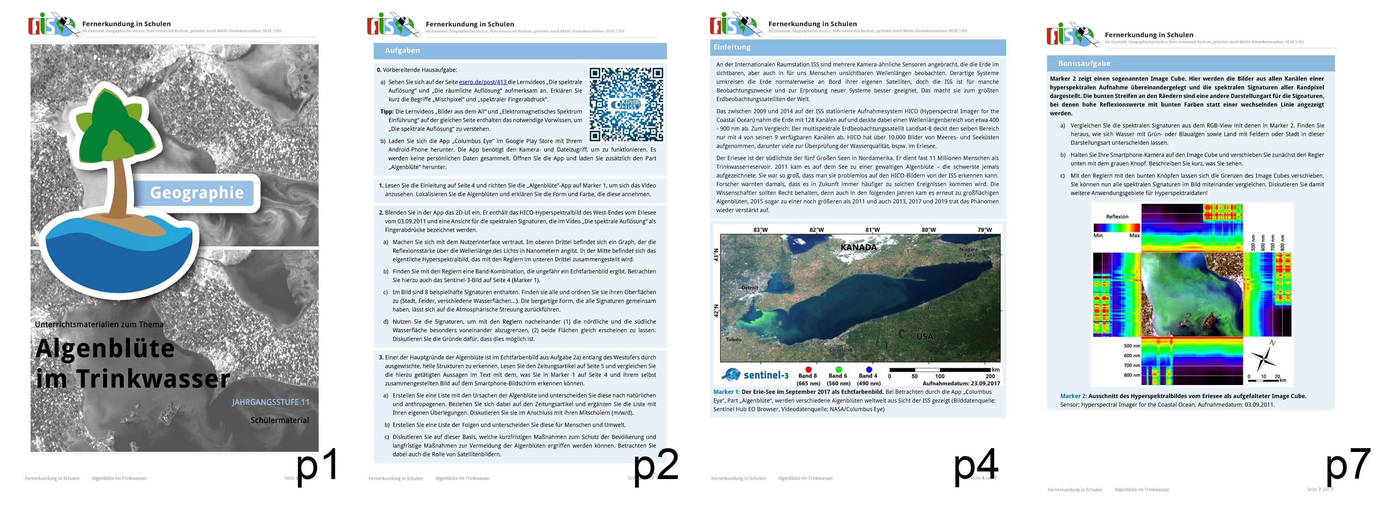The app is to be downloaded at home in case there is no free sufficient Wi-fi at school (Figure 13 p1).

In the first task, the students are to read the introductory text on the sheet and watch the short AR video about algal blooms all over the world (Figure 13 p4). While the 3D approach to displaying the 2D video in AR does not add anything of value in itself, it introduces the students to the principle of AR, overlaying animated information on the static worksheet. The video serves to show that algae blooms are not uniformly distributed in large bodies of water but depend on the properties of the different currents and the composition of additives.

The second task focuses on the hyperspectral data. It starts with the 2D user interface (UI) of the app with three color sliders to introduce them to hyperspectral data and red, green, and blue (RGB) image composition (Figure 10). The students are expected to become familiar with the UI before they have to combine the bands into a true color image.

As they have learned from the videos in the preparatory task what spectral signatures are, the students are now to find eight in the image and assign them to their surfaces (Figure 9 and Figure 11). Finally, the two main “types” of water need to be distinguished with those spectral signatures and their differences discussed.

The third task is entirely content based. The students are to read a news article about the algal bloom in question and compare the reasons for the extreme bloom from the text with what they can see in their own image in the app. These reasons are sorted into natural and anthropogenic with their own ideas expanding the lists. Consequences for humans and the environment are to be listed. Based on these lists, students are to come up with measures to protect the people and the environment in both the short- and long-term and include how satellite imagery can help with these tasks.

The fourth task brings all of the information together and introduces students to the method of distinguishing between harmless and potentially harmful algae with hyperspectral imagery. The students are to read an information text about the differences between green and blue algae and how their pigments, chlorophyll a and phycocyanin, can be differentiated using images of high spectral and high spatial resolution. They are also introduced to the toxin produced by the algae in this specific algae bloom, microcystin. Together with the information from the videos earlier, the students are to discuss how images of different spatial and spectral resolution yield different results. Through the app, they can see two maps of algae concentration derived from the HICO data in Lake Erie in 2011 (Figure 14) and the Landsat image. The virtual content replaces the on-screen zoom function, so the students can see details in the maps by moving their smartphone closer to the marker image. This allows them to see each pixel in the small maps as well as the very large Landsat image that spans more than one A4 sheet to provide a high resolution.

Based on all the knowledge gained so far, the students can now interpret the maps and satellite images. Five points are marked in the maps where the students have to make decisions on what to do as a local government under the given circumstances. One of them is the water extraction point for the City of Toledo, three are beaches with very different algae concentrations, and one is an area exemplary for commercial fishing.

In an optional task, students are introduced to a different way of displaying hyperspectral data: the image cube, in which light intensity is colored in rainbow colors. In this case, it is an image stack (Figure 12). The tasks are to compare this way of hyperspectral display with the one from the RGB slider view, familiarize themselves with the options in the UI, and discuss other topics hyperspectral data could be useful for in this image.

2.5. Teacher Material

Earth observation is not necessarily covered in geography education studies, nor those of any other subject. While the use of smartphones and AR in school lessons is on the rise, it is far from ubiquitous [52]. Hence, the teacher material needs to be extensive, explaining every step the students have to undertake and vast background information to be able to answer questions that might come up. The material includes a lesson plan in which the teacher is advised when to organize students into groups that use the app together to discuss certain tasks, or do some tasks at the black or white board with the entire class, furthering communication within the class. These are entirely advisory, depending on factors such as prior knowledge, class size and available mobile devices; they can and should be changed to better fit the needs of the class. In particular, the level of prior knowledge in the class is important for how much time the preparatory videos and possible explanation of biology components will take in the lesson. Sample solutions for each task are also given with extensive background information about the actual event in Lake Erie in 2011 and the methodology used for this study, as well as general tips about the app and advice on common mistakes.

2.6. Evaluation

A preparatory questionnaire for previous knowledge was developed, testing whether the students have used satellite imagery (especially hyperspectral imagery), digital learning, and mobile learning before. Another question was about curricular context, to ensure the topic fits into the curriculum and the students have some previous knowledge of it.

The preparatory questionnaire was a standardized, closed multiple-choice test where students could choose statements on how often or how intensively they have used certain media or studied certain topics. For the final evaluation, a fully standardized, written questionnaire with “yes/no” answers was chosen [53], mainly due to the time, as the evaluation has to fit into the same lesson as the use of the app to avoid changes in perception over time and using only an appropriate amount of time for the students [54]. A field to add free text was also added to see if the students had any additional comments.

The evaluation’s overarching goals are to find out:

• whether the students can understand how the complex hyperspectral data is used
• whether the students are able to use and understand the contents of the app intuitively
• how to improve the worksheet and app

It is thus both summative and formative in nature [55]. There is no control group, as no other learning material using and explaining hyperspectral data could be found and this is the central question of this study.

The evaluation takes the holistic framework by [49] into consideration but is reduced due to the aforementioned time constraints. The material fulfils the conditions for “didacticized” material, that is “characterized by combining tools and tests and facilitating learning and teaching: including textbooks, online teaching materials, and educational games” [49]. The potential learning includes both primary skills, or what the students learned, and secondary skills, or how the students used the materials. The former is tested by including many questions about the understanding of the hyperspectral data and its uses. As the latter is only detectable in the final task, where students have to read the microcystin maps to make spatial decisions, this is tested with their understanding of this task.

The actual learning potential is based on the ways that students communicate while using the learning material, including communication with the teacher, each other, and media. As is written in the teacher material, several tasks are to be performed in small groups and discussed in the class. The solutions to the tasks are not universal and allow for the students to come to different conclusions if the teacher decides to follow this recommendation. Only the communication with the media, which is the app, was tested in the questionnaire, by asking how well students subjectively understood the individual app parts and whether these added value to the worksheet. The results of the questions on understanding are reinforced with objective questions about the content of the worksheet and app. The temporal considerations of the actual learning potential are an inherent part of the worksheet in the form of the workflow described in Section 2.2.

The actual learning outcomes can be divided into three categories: intended learning, unintended, but valuable learning, and unintended and undesirable learning [49]. The intended learning includes facts about the algal bloom in question, about hyperspectral data, and certain soft skills, as defined in Section 2.1, and can be determined in the closed questionnaire. Unintended learning, whether valuable or undesirable, is harder to determine. The “wrong” questions in the questionnaire aim to find misunderstandings and wrong assumptions. Some of the right questions are also above what would be expected of students this age to determine valuable, but “unintended” learning. True unintended learning cannot be determined with closed questions but can be observed by an onlooker.

For each of the five tasks in the worksheet, five “yes/no” questions were chosen to see if the basics were retained or whether there were misconceptions. These tasks can be summarized as: hyperspectral data, spectral signatures, use of hyperspectral data on algal blooms, microcystins (Figure 10, Figure 11 and Figure 14), and image stack (Figure 12). The questionnaire was presented to several experts from the field of geography didactics and geomatics where it was discussed and improved.

The app was evaluated in March 2020 with two advanced geography courses at the Gymnasium Siegburg Alleestraße (ger. “Gymnasium” is an academically oriented grammar school). The school lies in the city center of Siegburg near the former German capital Bonn and has a diverse student body with children from all socio-economic backgrounds. The two courses were:

• Course “Q1”: year 11 (Q1: “Qualifikationsphase 1”—second-to-last year of high school as qualification phase for the Abitur (high school diploma)), 18 students were present, 9f/9m
• Course “Q2”: year 12 (Q2 (“Qualifikationsphase 2”—final year of high school and qualification phase, ends with Abitur)), 18 students were present, 9f/9m

For comparison, the written grades of the students in the same term were acquired fully anonymized in accordance with the school’s strict privacy protection guidelines. Grades from other subjects were not acquired as only very few students took any of the relevant ones (e.g., physics, biology) in the same year. Both courses are taught by the same teacher, who works in close cooperation with the project and regularly uses satellite imagery in her classes for nearly every topic. The school follows very strict anonymization standards and, as such, no data that could be traced back to any individual student could be acquired.

The app and worksheet developer was present for the test lessons to take additional notes, such as unintended learning not covered in the questionnaire, and to help with technical problems, but did not engage with the students in any other capacity. Notable subjective observations by the developer include: (1) The students were excited by using their smartphones in class but even more so about having handouts printed in color; (2) The students had no problems using the technology in itself and were better organized than the teacher regarding quick adjustments (like opening a Wi-Fi tether for fellow students to download materials) or just trying the app content out and experimenting with it; (3) Especially, the RGB image seemed a fun thing to play around with and create something “artsy” with the channels, but students also wanted to know why the colors changed as they did; (4) The students seemed unusually motivated to take part in the lesson. All chatter overheard in the class was about the topic and no student was caught using their smartphone for anything but the app.

3. Results

The project app was published on the Google Play Store at [56] with the algal bloom part being initially released in June 2019 and presented at the EARSeL Symposium in Salzburg, Austria. Subsequent updates until the evaluation in March 2020 saw improvements in data handling and UI intuitivity. Only minor adjustments to the app part were made afterwards. The app received an update to Unity 2019 in version 2.0, released in August 2021 due to the Google Play Store requirement to allow for 64-bit processing. The main functions described here were not affected.

In the evaluation, the short preparatory questionnaire revealed that only a few of the students were aware that they worked with satellite imagery on a regular basis: although according to the teacher, it had been part of their lessons, 25% had never heard the terms multispectral or hyperspectral to the extent that they put an extra remark on the questionnaire one step further than “I have never dealt with [multi- or hyperspectral data] before”. Of the rest, only three students had ever knowingly dealt with multispectral data and only one with hyperspectral data. It is important to note that this does not mean the students had never used an RGB satellite image, only that they were not aware of it. The answers showed that educational apps were used in this class occasionally (according to the teacher: the other project apps [57], again emphasizing that the students do work with satellite images regularly). Although this class had desktop computers readily available in their classroom, working with mobile devices happened more often than on those. The lack of desktop computer use was summarized by the students as the devices and the internet being too slow and too restrictive at this school (i.e., digital materials get deleted randomly, even teaching websites are blocked sometimes). The answers also showed that students have learned about the overarching topic of the app, which is environmental problems due to agriculture, in their regular lessons. The fact that environmental problems from agriculture are part of the regular curriculum is important for the usability of the app, as teachers rarely have time to incorporate off-curriculum topics into their lessons.

The app was tested in regular two-hour lessons (plus a 5 min break in between) with each class, resulting in 95 min total for settling down, working with the worksheet and app, and evaluating it.

In the Q2 group, most students admitted to not having watched the introductory videos, which was then done on their private smartphones, but took away a valuable 15 min from the allotted time. Thus, there was not enough time to finish the fourth and final task for many students and not even time to look at the optional task at the end. In Q1, most had seen the videos and were sufficiently prepared. Thus, most students finished the fourth task and a few spent the time waiting until they could compare it with their peers when doing the optional task.

Despite not having completed all of it, many students completely filled out the questionnaires. Answers that cannot be anything but guessed, because the students of the respective group did not reach that stage, were excluded from the results. Hence, the last set of questions is only given for Q1.

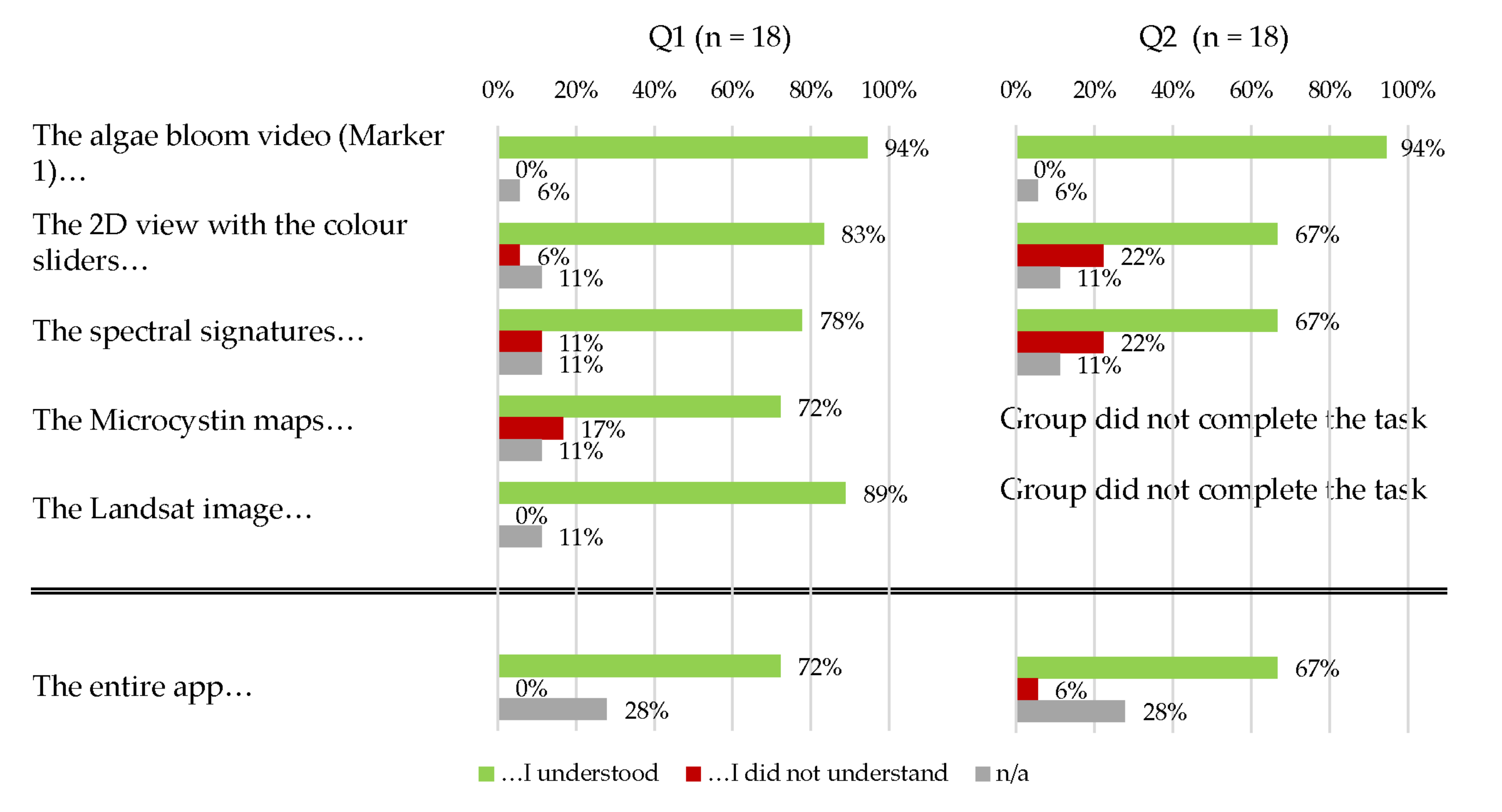
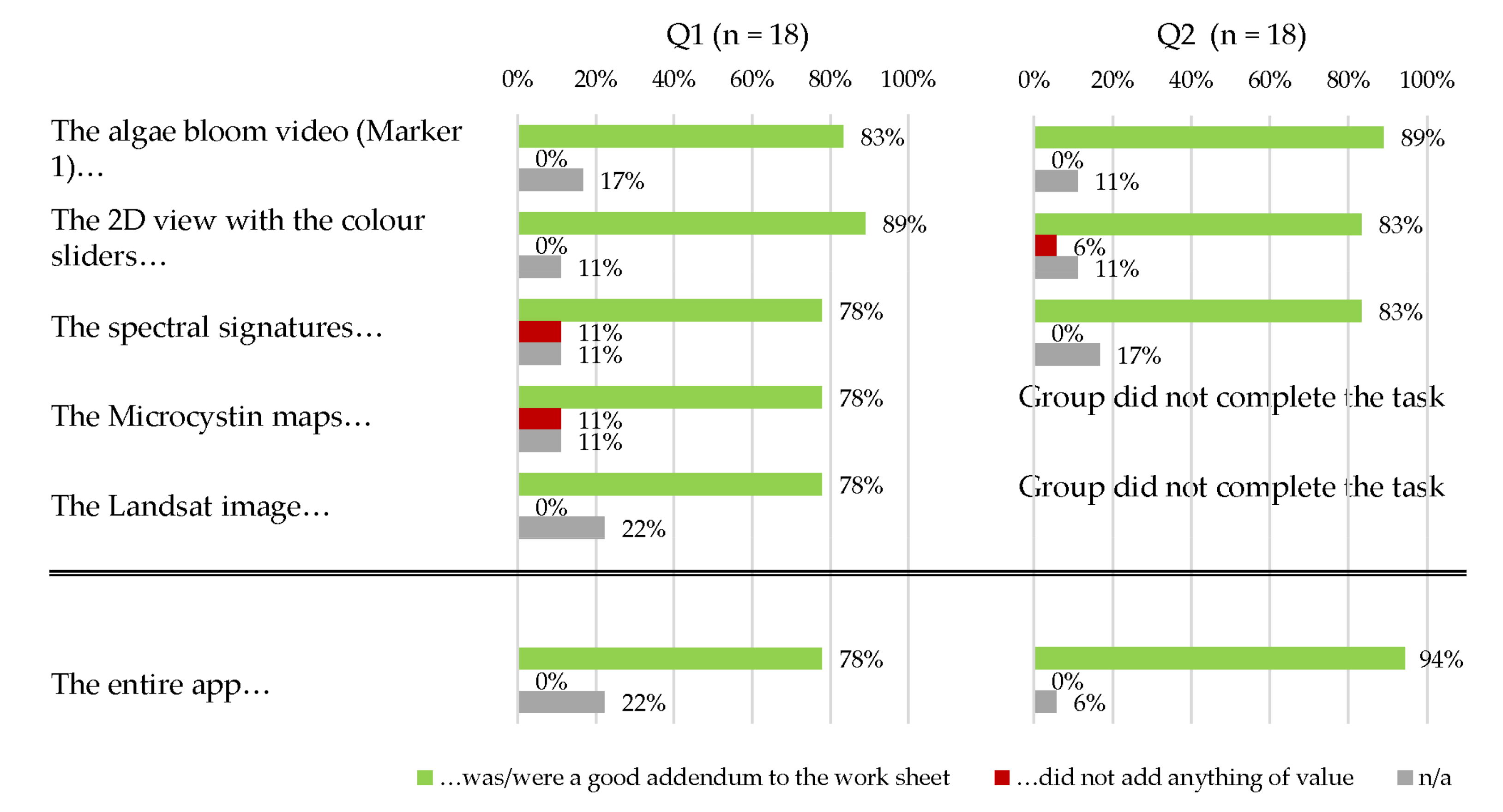
The final evaluation shows that the app worked for most students, as long as they had Android phones, as the app does not exist for iOS yet. These students partook in the lesson in small groups with the Android users. In the subjective part (see Figure 15 and Figure 16), most students claimed to have understood what was going on in the individual parts of the app and considered the app a good addition to the worksheet.

The objective part of the evaluation supports their answers:

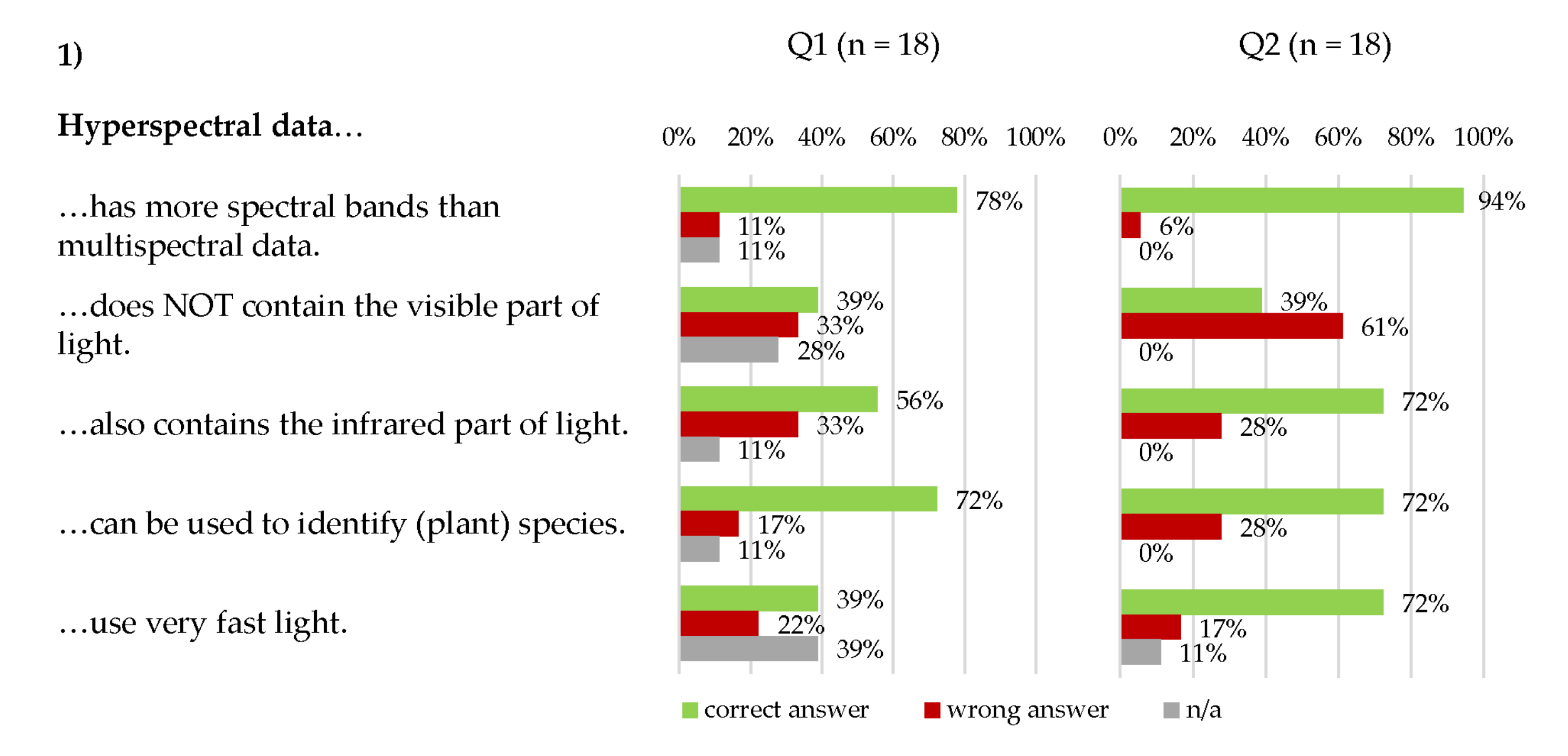
• The questions about the properties of hyperspectral data (Figure 17) were answered correctly by the majority. The only question that was problematic was whether hyperspectral data contain the visible part of the electromagnetic spectrum:
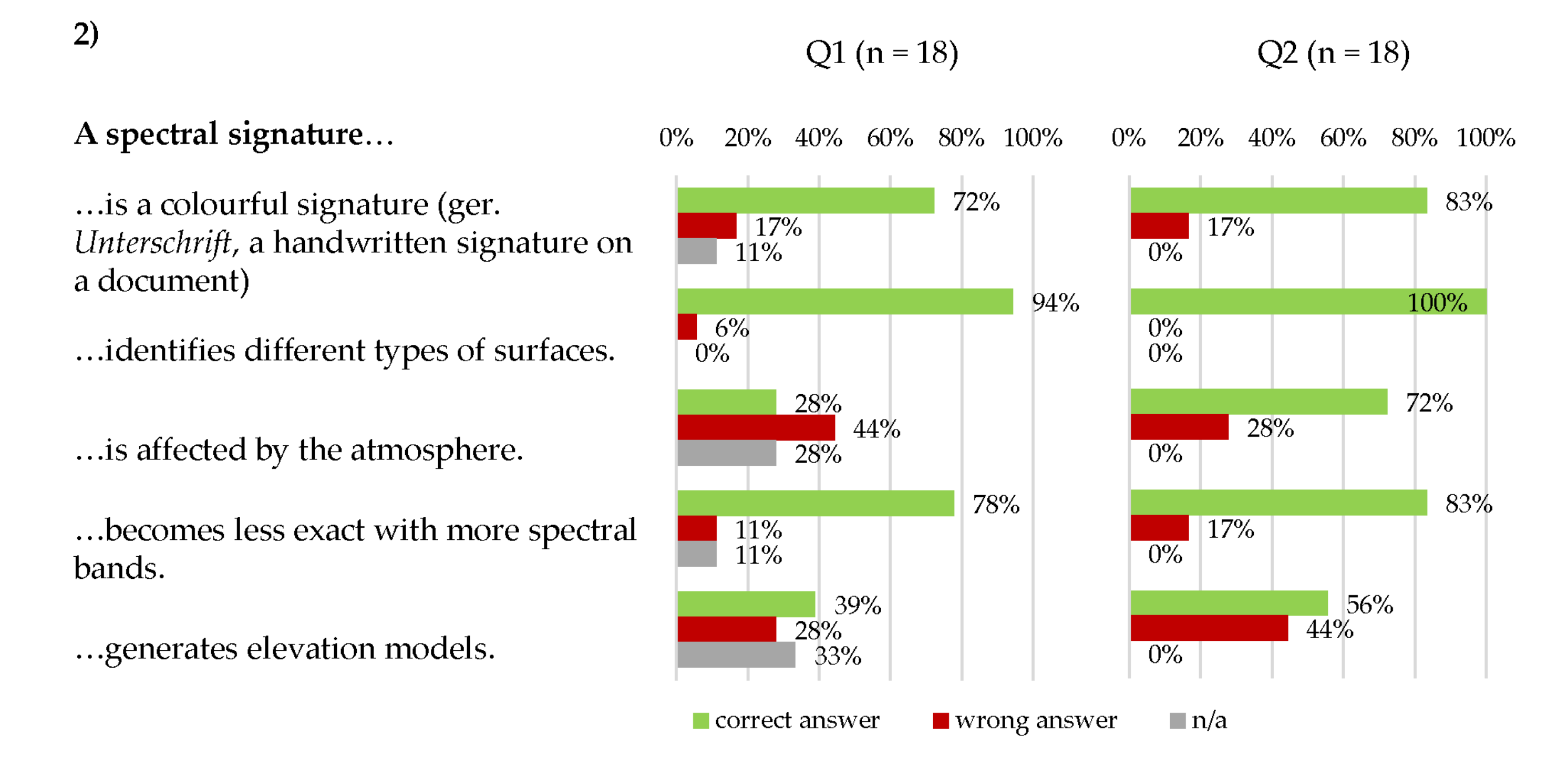
• The part about spectral signatures (Figure 18) proved more problematic as the students did not have the required prior knowledge about atmospheric scattering and did not know what an elevation model was (according to the teacher, these topics are described as necessary prior knowledge in the teacher material, though, and examples for teaching materials are given). The other three questions however were rarely answered incorrectly:
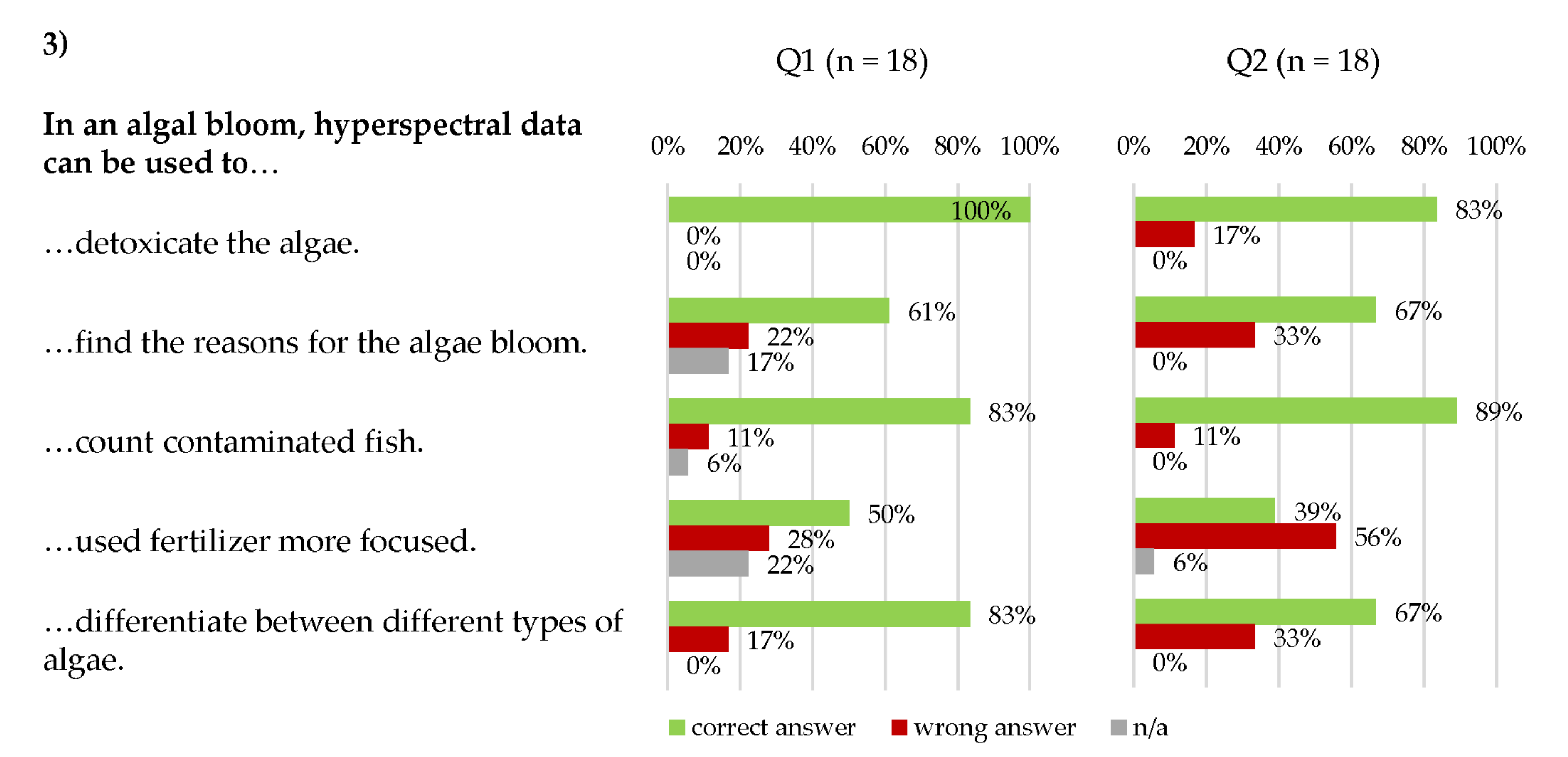
• The questions about using hyperspectral data for the analysis of algal blooms (Figure 19) revealed a good understanding of the possibilities. The only problematic question was whether hyperspectral data can help to use fertilizer in a more focused way: Many students thought this was possible:
• Several students answered these two parts (spectral signatures and the use of hyperspectral data in algal blooms) entirely, or almost entirely, correctly.
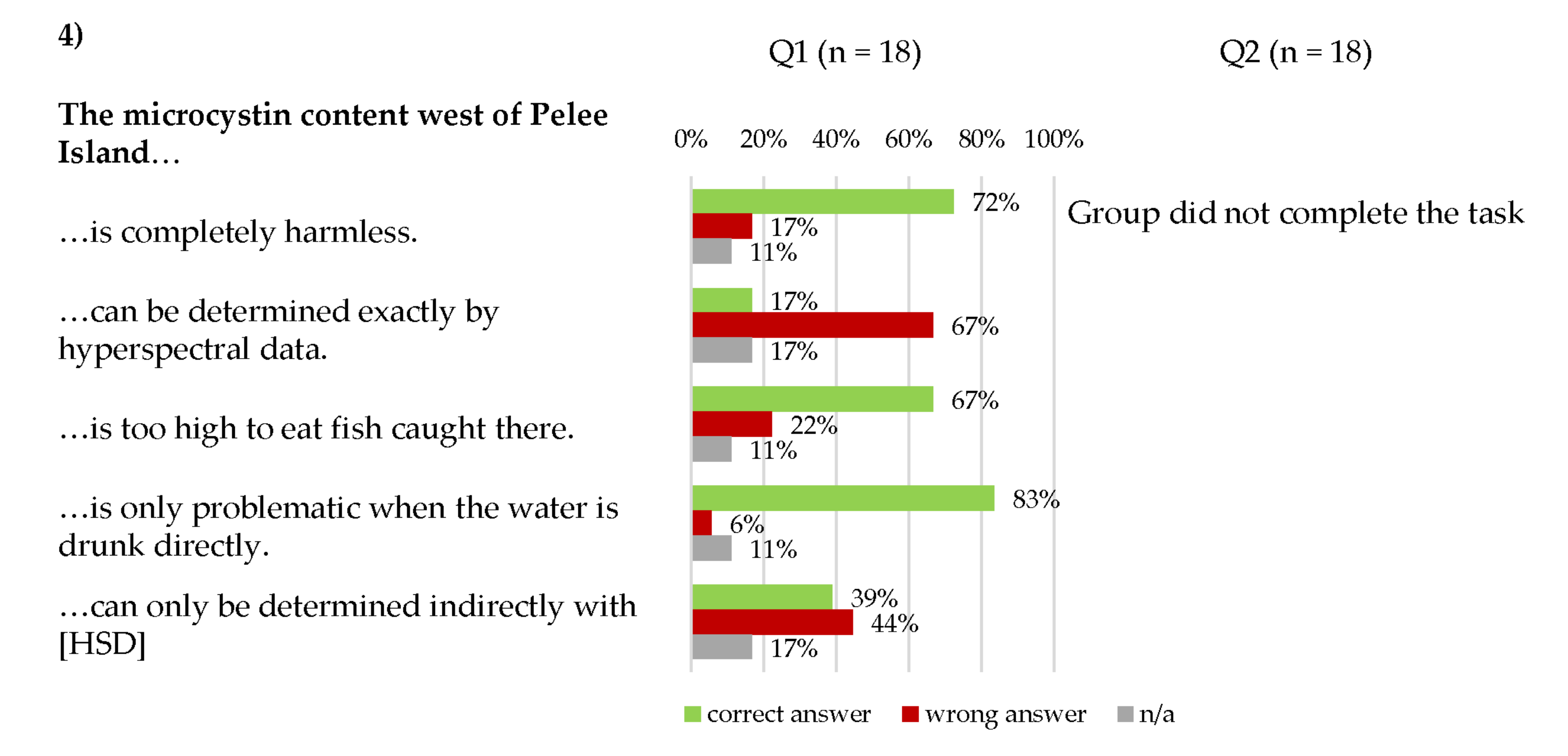
• Only the Q1 group had the time to do the fourth task and, thus, the questions about this part were only evaluated from that group (Figure 20). Students came to the correct conclusion about the content of toxic algae but thought the hyperspectral data could determine the exact amount of the toxin, when the worksheet should have taught them that there are several ways to approximate the content from hyperspectral data.
• The question about the image cube were only answered by up to eight students and therefore were not included here. These complained that the cube was stuttering, i.e., bringing their devices to their limits.

Figure 17. Answers from both test groups about the properties of hyperspectral data.

Figure 17. Answers from both test groups about the properties of hyperspectral data.

Figure 18. Answers from both test groups about the properties of spectral signatures.

Figure 18. Answers from both test groups about the properties of spectral signatures.

Figure 19. Answers from both test groups about the use of hyperspectral data in algal blooms.

Figure 19. Answers from both test groups about the use of hyperspectral data in algal blooms.

Figure 20. Answers from Q1 group to determine whether they understood the conclusive task that combines all knowledge gathered through the worksheet and app.

Figure 20. Answers from Q1 group to determine whether they understood the conclusive task that combines all knowledge gathered through the worksheet and app.

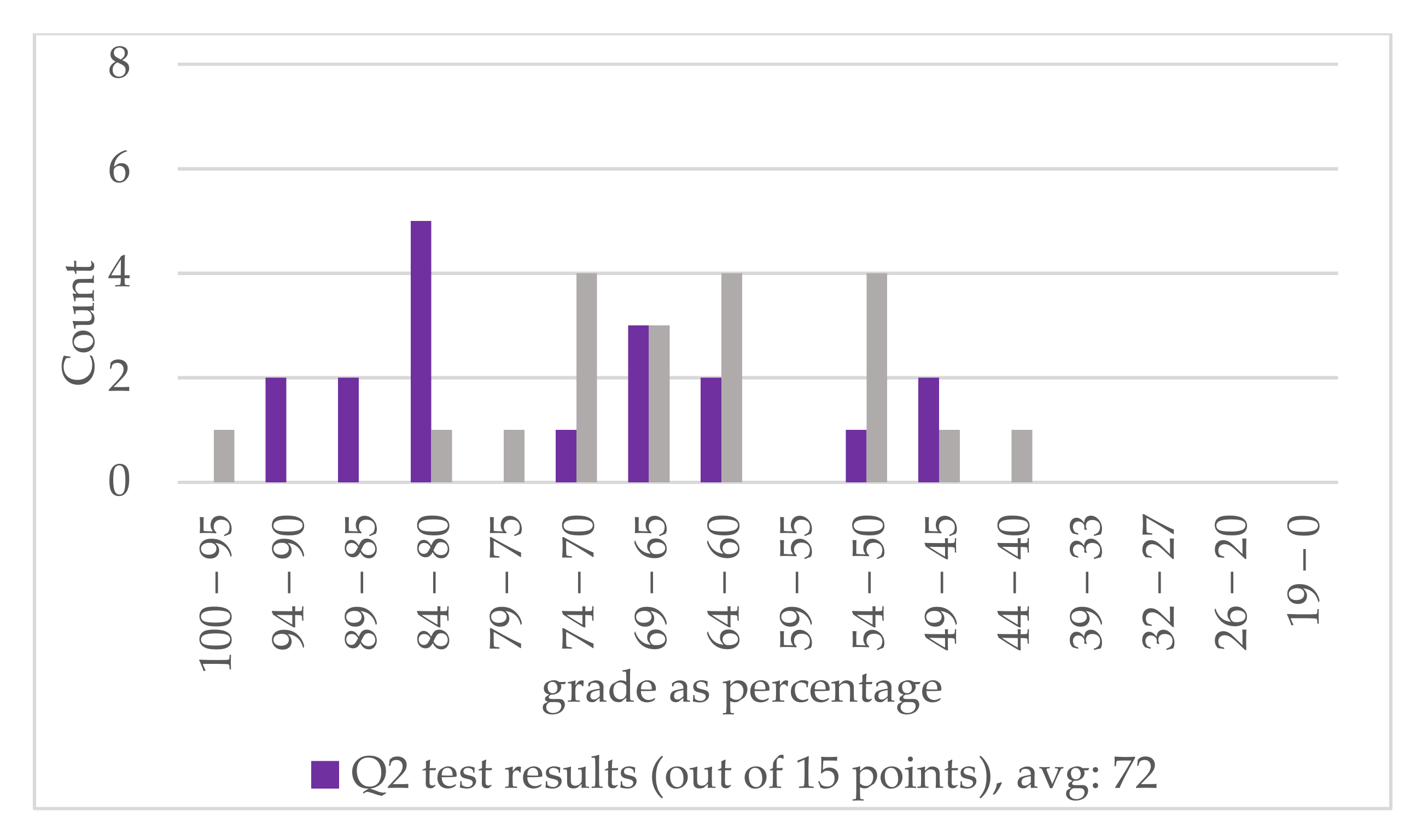
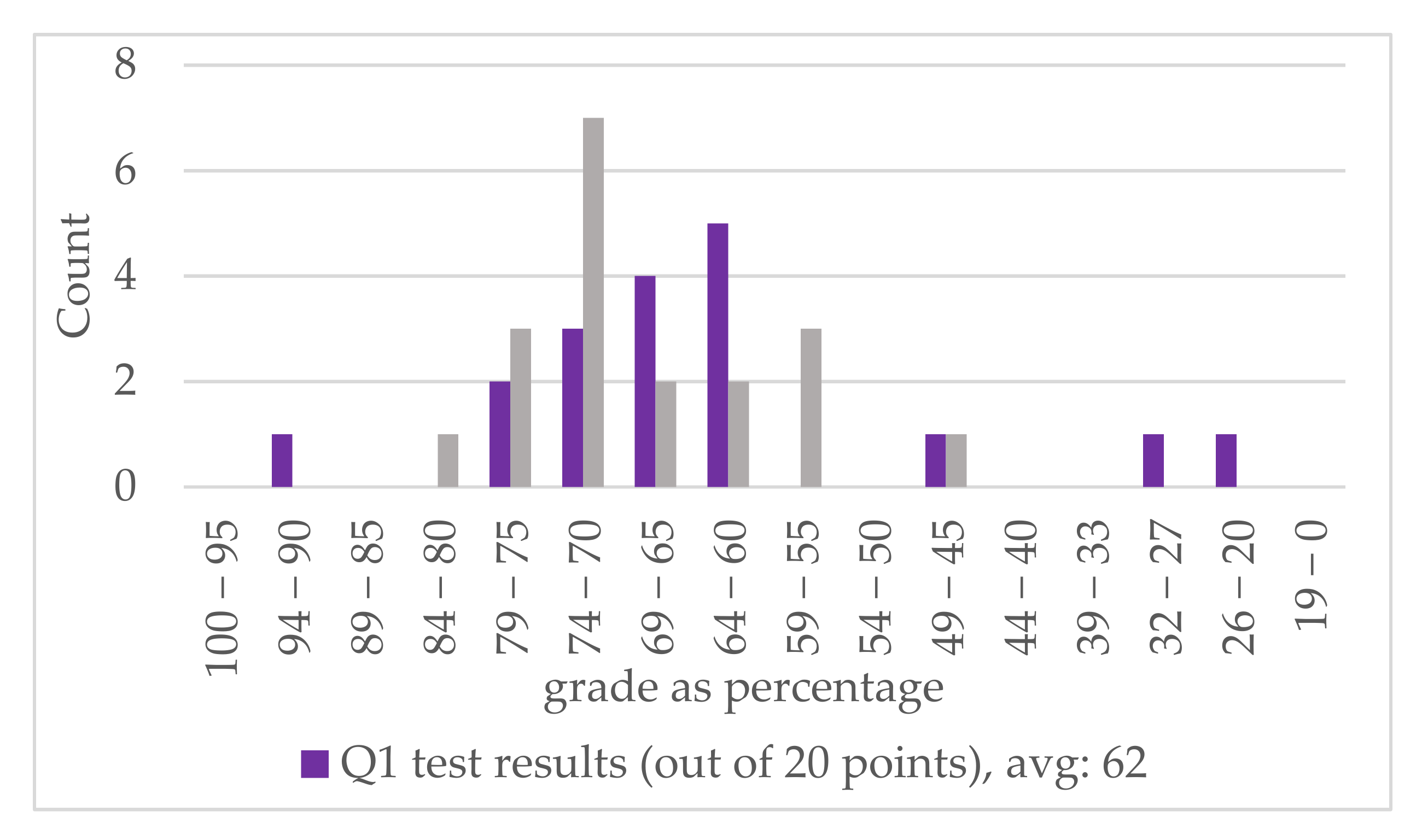
In comparison with their written grades in the rest of the semester, Q1 performed slightly worse in the evaluation and Q2 slightly better (Figure 21 and Figure 22). The written grades are an average of all written exams per student in the semester. There were more students in the “very good” range (100 to 85%) in both tests than through the average written grades, but the only two failing grades (<40%) were also from the tests. Due to the high anonymization standards of the school, no direct comparison between individuals could be drawn.

4. Discussion

The worksheet was timed well for a 90-min lesson if the preparatory task was performed by the students. The desired primary skills were acquired by the majority of students and secondary skills furthered, including the use of technology. The students were able to work with the given media and could follow the workflow of the worksheet and app. The majority of students learned what was intended, but some answers revealed unintended, undesirable learning as well. Unintended, valuable learning was not observed. From this, we deduce that many students in the group understood the basics of using hyperspectral data, and its uses, but not its limitations. The topic is thus understandable for the students to a degree that is expected at their level. Comparing the scores from the evaluation with the average written grades of the students showed that the Q1 performed slightly worse (6 percentage points) with the app and the Q2 slightly better (7 percentage points) than their written tests in the same semester, indicating no major problems with the worksheet. The teacher considered the worksheet very challenging for the students, but doable under the condition that there were students who were taking biology classes in that same year. A major remark was that there was too much text in the worksheet. In the subsequent version, the very long introductory text of the fourth task was broken down and shortened. The lesson plan in the teachers’ material is, though, only a recommendation and so are parts of the sample solutions. Different classes taught by different teachers will thus differ in their achieved learning.

The data used in this study was, at the time of the development of the app, not easily available with atmospheric correction. This led to problems both in the RS research part as well as the understanding part for students, who may have had to handle too much information at once when learning about the hyperspectral data. A future iteration should utilize atmospherically corrected data. The app itself, or its individual functions, can easily be reused with other data. More applications for hyperspectral data could thus be implemented according to the official curricula and available data from other hyperspectral sensors.

The evaluation is sufficient to show whether the topic was understandable for students at all, but has limitations on further details, mostly due to the sample size and the high degree of anonymization required by the school. A long-term evaluation on how much students have retained from the worksheet at the end of the year, or how it changed their perception on any of the topics within, should be performed in the next iteration. Due to the lack of a comparison group, the results are only partially informative. If similar materials without the AR, or any digital, component are created in the future, a comparison with the material evaluated here would be beneficial.

5. Conclusions

The massive harmful algal bloom in Lake Erie in 2011 served as a topic to create a worksheet and app for German school lessons that used freely available hyperspectral data for a STEM lesson on how such data is used in determining anthropogenic influences on natural habitats. Two maps of microcystin content (Figure 7 and Figure 8), derived from different pigments, could be produced from September 2011 HICO data at the height of the algal bloom. Spectral shape algorithms were adjusted to optimally detect chlorophyll a and phycocyanin as proxies for all photosynthesizing matter and potentially microcystin-producing cyanobacteria. Discerning the two pigments was possible, but an accurate correlation with in situ measurements was not possible due to inconsistencies with measurement dates from the sensor and in situ. Despite the large variances in the correlations and data uncertainties, the maps showed a significant difference in pigment distribution, and therefore algae distribution and thus possible toxin distribution.

In order to create an app with the data, the HICO data set was reduced from 591 MB to 18 MB by cutting or clipping bands and reducing bit depth, and from a format only readable by certain GIS to ubiquitous PNG format, allowing for implementation in an app useable by smartphones but losing a lot of information in the process. Current hyperspectral sensor data, such as DESIS with its more than 200 bands, may be too much to handle for current devices, even when reduced. Any information depending on high accuracy of the radiometric resolution, such as the spectral signatures of interesting points, or the data for image calculations, had to be extracted prior to the data size reduction. Two different visualization methods for the hyperspectral data using minimal computing power were developed using HLSL shaders, the RGB viewer (Figure 10) and the image stack (Figure 12). The RGB viewer is to display the R, G, and B parts individually from greyscale images, resulting in instantly combinable RGB images. The image stack is an enhancement of the image cube, in which the borders on which the spectra are displayed are instantly adjustable through user input. While the first does not necessarily need AR, the second benefits from the 3D visualization bound to an object in the real world that serves as an explanation for how it works as much as a means to turn the stack around. The maps derived from the two different pigments to show potential toxin distribution (Figure 7 and Figure 8) in the lake were also included, since calculating and rendering them live on the users’ smartphones was considered too processing power intensive, and too complex a topic given the prior knowledge of the target group. The main benefit of the maps in an app versus printed material is that a wide range of colors can be used and will not be affected by the printing capabilities, but the AR improves zooming in and out by moving the smartphone closer or further away from the image target. The included video benefits from the AR in the same way—thus, it serves as an easy introduction into AR for the users. The app with all the intended features is published in the Google Play Store [56] and the worksheet is made available through the project’s website [57].

The game development environment Unity requires additional functions and shaders to be used with hyperspectral data on smartphones. This includes the visualization of such data, as they are too large to be processed on mobile devices at the moment. The data therefore have to be pre-processed and selected to minimize both data volume and processing power. Smartphone apps can be utilized to display colorful, animated content not otherwise printable in schools. AR can make up for deficiencies of mobile devices, such as small screens, and even create possibilities in 3D that are not possible on 2D screens. However, the required processing power for AR is already high, and the processing power for the many bands of hyperspectral data brings some devices to their limits. The data have to be reduced in size, visualization methods adjusted, processing eliminated, and all processing steps performed prior to implementation.

Considering all these restrictions and possibilities, it is possible to implement hyperspectral data into an AR app, as long as the original data is not required, which is the case for educational apps. The app developed in this study shows that it is possible to convey complex RS data and methodology in a simplified manner to high school students and at the same time as conveying knowledge about its application in ecological research and environmental protection.

The worksheet and app about hyperspectral data for the detection of harmful algae blooms in Lake Erie with real RS data and methods were doable for the students of the advanced geography courses, meaning hyperspectral imagery can be used in regular school lessons by use of AR on students’ smartphones. The students experimented digitally and performed research-like tasks on their smartphones, applying their prior knowledge from geography, physics, and biology to RS data in a real-world example, fitting into their regular curriculum that they need to complete to qualify for the Abitur. AR was used productively, using visualization methods not possible with printed materials alone, and even going beyond common GIS visualizations. The lesson could be performed by a teacher who uses satellite imagery and AR regularly, but it needs to be considered how teachers with less prior knowledge and experience in these fields would fare with the given materials. More apps of this kind using other sensors’ data will be created based on this model with options to use other complex data, such as InSAR, in curriculum-oriented lessons using AR. The app presented here will also be published in iOS within the first half of 2022.