An Adaptive Lp Norm Minimization Algorithm for Direction of Arrival Estimation

Abstract

In this paper, we propose a new direction of arrival (DOA) estimation algorithm, in which DOA estimation is achieved by finding the sparsest support set of multiple measurement vectors (MMV) in an over-complete dictionary. The proposed algorithm is based on ${\ell }_p$ norm minimization, which belongs to non-convex optimization. Therefore, the quasi-Newton method is used to converge the iterative process. There are two advantages of this algorithm: one is the higher possibility and resolution of distinguishing closely spaced sources, and the other is the adaptive regularization parameter adjustment. Moreover, an accelerating strategy is applied in the computation, and a weighted method of the proposed algorithm is also introduced to improve the accuracy. We conducted experiments to validate the effectiveness of the proposed algorithm. The performance was compared with several popular DOA estimation algorithms and the Cramer–Rao bound (CRB).

1. Introduction

With extensive applications, including radar, sonar, wireless communication and remote sensing, DOA estimation has traditionally been a popular branch in the field of array signal processing [1,2]. As a key technology in passive radar, DOA estimation is being extensively developed to locate targets in complex electromagnetic environments without being perceived.

Considering problems, such as distinguishing coherence sources and separating spatial closely sources, sparse reconstruction theory plays an important role in DOA estimation [3,4]. In dividing the whole spatial domain of interests into a discrete set of potential grids, a traditional estimation module can be converted into an ill-posed inverse problem. The specific physical model will be introduced in Section 2.

The MMV data module of a M sensor array takes the following form:

$$\mathbf{Y}=\mathbf{AX}+\mathbf{N}$$

(1)

where $\mathbf{Y}\in {\mathbb{C}}^{M\times L}$ and $\mathbf{N}\in {\mathbb{C}}^{M\times L}$ are matrices of measurements and noise. The dictionary matrix $\mathbf{A}\in {\mathbb{C}}^{M\times N}$ consists of N steering vectors. These vectors are determined by N different angles. In addition, $\mathbf{X}\in {\mathbb{C}}^{N\times L}$ is a K-row sparse matrix that represents a K sources spatial spectrum.

Note that the dictionary matrix $\mathbf{A}$ is fat; hence, the equation $\mathbf{Y}=\mathbf{A}\mathbf{X}$ has infinitely many exact solutions. To reconstruct the sparse signal, a simple and intuitive measure of sparsity is ${\ell }_0$-norm. The Lagrangian relaxation problem with the ${\ell }_{2,0}$ mixed norm is as follows:

$$\underset{\mathbf{X}}{min}{\parallel \mathbf{Y}-\mathbf{AX}\parallel }_F^2+\lambda {\parallel \mathbf{X}\parallel }_{2,0}$$

(2)

Note that the mixed-norm ${\parallel \mathbf{X}\parallel }_{2,0}$ means a sparse spatial domain but closely related time domain. That is to say, ${\ell }_2$ norm gathers the snapshots of $\mathbf{X}\in {\mathbb{C}}^{N\times L}$ to obtain a spatial spectrum ${\mathbf{X}}_{vec}\in {\mathbb{C}}^{N\times 1}$, and ${\ell }_0$ norm measures the sparsity of ${\mathbf{X}}_{vec}$. The general formula is:

$${\parallel \mathbf{X}\parallel }_{p,q}=\sum _{i=1}^N{\left(\sum _{j=1}^L{\left|{\mathbf{X}}_{i,j}\right|}^p\right)}^{q/p}$$

(3)

Considering solving (2) directly is an NP-hard problem, alternative approaches are often studied. One alternative method is the greedy algorithm, OMP [5] pursued the current optimal value in every iteration. Another method is an approximate ${\ell }_0$ norm method, such as SL0 [6].

A common convex approximation of the ${\ell }_{2,0}$-pseudo-norm that is known to promote sparse solution is the ${\ell }_{2,1}$-norm.

$$\underset{\mathbf{X}}{min}{\parallel \mathbf{Y}-\mathbf{AX}\parallel }_F^2+\lambda {\parallel \mathbf{X}\parallel }_{2,1}$$

(4)

Convex optimization algorithms are always convergent to the global optimal solution. This feature makes convex optimization algorithms well-studied. Malioutov et al. proposed a heuristic approach, named ${\ell }_1$-SVD [7], using a reduction of the dimension of measurement matrix $\mathbf{Y}$ by SVD and adaptive grid refinement. However, for a large number of snapshots L or large number of candidate frequencies K, the problem becomes computationally intractable.

Different from other sparse reconstruction fields, in the DOA estimation, atoms of dictionary $\mathbf{A}$ are completely determined and fixed by the discrete spatial grid. Highly correlated atoms in the dictionary makes it difficult to separate adjusted vectors. This is far from the “approximate orthogonality” condition, which was introduced in the Restricted Isometry Property (RIP) [8]. However, ${\ell }_p$ norm optimization has a greater possibility of obtaining a sparse solution, which is usually used in imagery target detection [9]. Thereby, ${\ell }_p$ norm optimization also can be used to distinguish closely spaced sources.

$$\underset{\mathbf{X}}{min}{\parallel \mathbf{Y}-\mathbf{AX}\parallel }_F^2+\lambda {\parallel \mathbf{X}\parallel }_{2,p}$$

(5)

Hence, in the ${\ell }_{2,p}$-constrained problem we search for an N-row sparse solution that minimizes the fitting error. Algorithms, such as iterative reweighted least squares (IRLS) [10] and FOCUSS [11] are popular in DOA estimation. They both approximate the ${\ell }_p$ norm with a weighted ${\ell }_2$ norm.

The goal of this paper is to find a practical sparse reconstruction method that fills the missing application scenario of traditional DOA estimation algorithm. The main contribution of the paper is a method for the automatic selection of the regularization parameter.

In contrast to other existing methods, the proposed method works completely in the iterative process, which means better adaptability to different situations. The key ingredient of the proposed method is the use of the quasi-Newton algorithm. Without losing accuracy, the iterative process is optimized, and the computation is reduced by a matrix inverse lemma, even with dense grids. In addition, we introduce the improvement of the weighted algorithm. Last but not least, the array does not have to be linear, and the sources can be coherent.

The rest of the paper is organized as follows. The processing of the proposed algorithm and innovative details are considered in Section 2. Potential application scenarios are discussed. Section 3 provides experimental results to compare the proposed algorithm with other DOA estimators. Our conclusions are contained in Section 4.

2. The Proposed Algorithm

The physical meaning of all parameters in the DOA estimation mathematical model will be explained here briefly. The array with all omnidirectional sensors receives plane waves from the far field of the narrow-band signal source. All signals ${\mathbf{s}}_k\left(k=1,2,\dots ,K\right)$ are impinging with different angles ${\theta }_k\left(k=1,2,\dots ,K\right)$. The phase difference between two adjacent sensors is defined as

$$\Delta {\phi }_k=2\pi \frac{dsin{\theta }_k}{{\lambda }_s}$$

(6)

where ${\lambda }_s$ denotes the wavelength. Let the sensor at the coordinate origin be the reference. The direction vector can be expressed as $\mathbf{a}\left({\theta }_k\right)={\left[1,exp\left(-j\Delta {\phi }_k\right),\dots ,exp\left(-j\left(M-1\right)\Delta {\phi }_k\right)\right]}^T$, and thus the manifold matrix can be expressed as ${\mathbf{A}}_s={\left[\mathbf{a}\left({\theta }_1\right),\dots ,\mathbf{a}\left({\theta }_K\right)\right]}^T$.

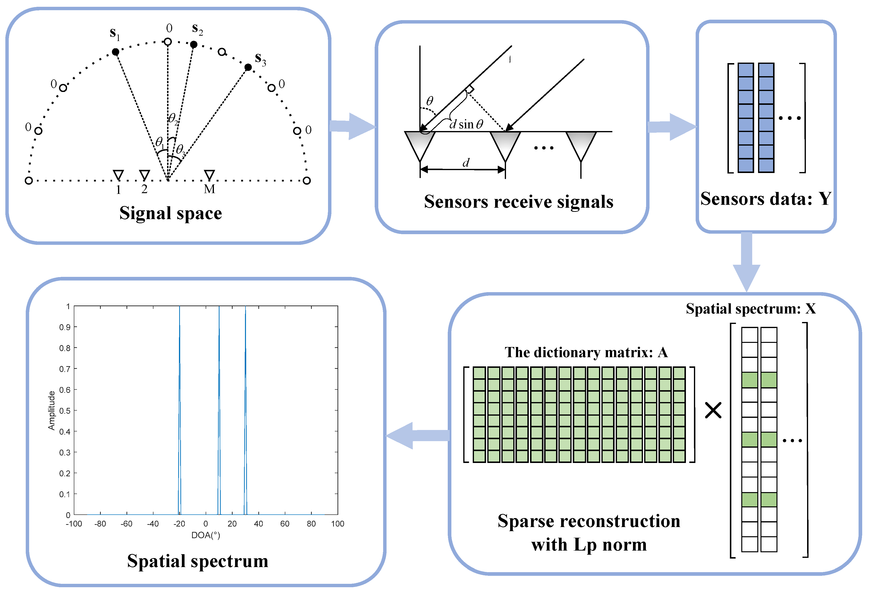
Figure 1 shows the whole processing of DOA estimation. In order of the subplots, first, the signal space can be divided to N grids; therefore, the dictionary matrix $\mathbf{A}$ can be expressed as $\mathbf{A}={\left[\mathbf{a}\left({\theta }_1\right),\dots ,\mathbf{a}\left({\theta }_N\right)\right]}^T$. Then, the sensor data matrix $\mathbf{Y}\in {\mathbb{C}}^{M\times L}$ is the input data of the proposed algorithm. M denotes the number of sensors, and L denotes the number of samples. Finally, with a proper coefficient, linear combinations of atoms in the dictionary can reconstruct the signal. As long as the sparsest coefficient vector can be found, the direction of sources can be known from the index of the non-zero support set.

Figure 1. Schematic of the DOA estimation process.

2.1. The ${\ell }_p$ Norm Minimization Algorithm

Due to ${\ell }_p(0<p<1)$, cost function (5) is not differentiable at $\mathbf{0}$. The authors in [12] proved a differentiable approximation suiting our purpose well:

$${\parallel \mathbf{X}\parallel }_{2,p}\approx \sum _{i=1}^N{\left(\sum _{j=1}^L\left|{\mathbf{X}}_{i,j}\right|+ϵ\right)}^{\frac{p}{2}}$$

(7)

where $ϵ\ge 0$ is the smoothing parameter that controls the trade-off between smoothness and approximation. Usually the value of $ϵ$ is set to ${10}^{-6}$ in the DOA estimation background. If $ϵ$ is too large, the approximation is not good, and if $ϵ$ is too small, the inverse of (11) will be singular.

Substituting (7) for ${\parallel \mathbf{X}\parallel }_{2,p}$ in (5):

$$F\left(\mathbf{X}\right)\approx F_{ϵ}\left(\mathbf{X}\right)={\parallel \mathbf{Y}-\mathbf{AX}\parallel }_F^2+\lambda \sum _{i=1}^N{\left(\sum _{j=1}^L{\left|X_{i,j}\right|}^2+ϵ\right)}^{\frac{p}{2}}$$

(8)

The Jacobian matrix of the objective function is

$$\begin{array}{c}\hfill \mathbf{J}=\left(2{\mathbf{A}}^H\mathbf{A}+\lambda {\mathbf{D}}_1\right)\mathbf{X}-2{\mathbf{A}}^H\mathbf{Y}\end{array}$$

(9)

where the superscript ${\left[•\right]}^H$ represents the conjugate transpose operation and

$${\mathbf{D}}_1={\mathrm{diag}}_{\left(i\right)}\left\{\frac{p}{{\left({\sum }_{j=1}^L{\left|X_{i,j}\right|}^2+ϵ\right)}^{1-\frac{p}{2}}}\right\}$$

(10)

The Hessian matrix of the objective function is

$$\begin{array}{c}\hfill \mathbf{H}=2{\mathbf{A}}^H\mathbf{A}+\lambda {\mathbf{D}}_1+\lambda {\mathrm{diag}}_{\left(i\right)}\left\{\frac{p\left(p-2\right){\sum }_{j=1}^L{\left|X_{i,j}\right|}^2}{{\left({\sum }_{j=1}^L{\left|X_{i,j}\right|}^2+ϵ\right)}^{2-\frac{p}{2}}}\right\}\end{array}$$

(11)

However, the Newton method is not convergent due to the non-positive definiteness of $\mathbf{H}$. A positive definite approximation of $\mathbf{H}$ can be obtained by simply removing the negative part in (11).

$$\begin{array}{c}\hfill \tilde{\mathbf{H}}=2{\mathbf{A}}^H\mathbf{A}+\lambda \left({\mathbf{D}}_1+{\mathbf{D}}_2\right)\end{array}$$

(12)

Note that

$${\mathbf{D}}_2={\mathrm{diag}}_{\left(i\right)}\left\{\frac{p^2{\sum }_{j=1}^L{\left|X_{i,j}\right|}^2}{{\left({\sum }_{j=1}^L{\left|X_{i,j}\right|}^2+ϵ\right)}^{2-\frac{p}{2}}}\right\}$$

(13)

In DOA estimation, the dimension of $\tilde{\mathbf{H}}$ is affected by the number of grids, usually $N\ge M$, which causes heavy computation. Considering $\tilde{\mathbf{H}}$ consists of ${\mathbf{A}}^H\mathbf{A}$ and a diagonal matrix $\lambda \left({\mathbf{D}}_1+{\mathbf{D}}_2\right)$, the matrix inversion lemma is introduced to optimize the inversion

$${\tilde{\mathbf{H}}}^{-1}=\left({\mathbf{Q}}^{-1}-{\mathbf{Q}}^{-1}{\mathbf{A}}^H{\left({\mathbf{I}}_k+{\mathbf{AQ}}^{-1}{\mathbf{A}}^H\right)}^{-1}{\mathbf{AQ}}^{-1}\right)$$

(14)

Note that

$$\mathbf{Q}=\frac{\lambda }{2}\left({\mathbf{D}}_1+{\mathbf{D}}_2\right)$$

(15)

Applying (14) can reduce the dimension of the inverse matrix from $N\times N$ to $M\times M$; thus, the computational complexity decreases to $O(N{M}^2+M^3+NM)$ from $O(M{N}^2+N^3+NM)$. In order to facilitate the subsequent measurement of residuals and introduce (14) to reduce the computational burden, the Newton direction ${\mathbf{N}}_d$ in the proposed algorithm can be expressed as:

$${\mathbf{N}}_d={\tilde{\mathbf{H}}}^{-1}\mathbf{J}={\mathbf{T}}_4-{\mathbf{T}}_3{\mathbf{T}}_4-{\mathbf{T}}_2{\mathbf{T}}_1+{\mathbf{T}}_3{\mathbf{T}}_2{\mathbf{T}}_1$$

(16)

where ${\mathbf{T}}_{1\sim 4}$ are repeated parts in calculating and ${\mathbf{T}}_1$ will be used to obtain the noisy parameter in section B.

$$\begin{array}{cc}\hfill & {\mathbf{T}}_1=\mathbf{Y}-\mathbf{AX}\hfill \\ \hfill & {\mathbf{T}}_2={\mathbf{Q}}^{-1}{\mathbf{A}}^H\hfill \\ \hfill & {\mathbf{T}}_3={\mathbf{T}}_2{\left({\mathbf{I}}_k+{\mathbf{AT}}_2\right)}^{-1}\mathbf{A}\hfill \\ \hfill & {\mathbf{T}}_4\left(i\right)=\frac{{\sum }_{j=1}^L{\left|X_{i,j}\right|}^2+ϵ}{\left(1+p\right){\sum }_{j=1}^L{\left|X_{i,j}\right|}^2+ϵ},i=1...N\hfill \end{array}$$

(17)

2.2. Adaptive Method for p

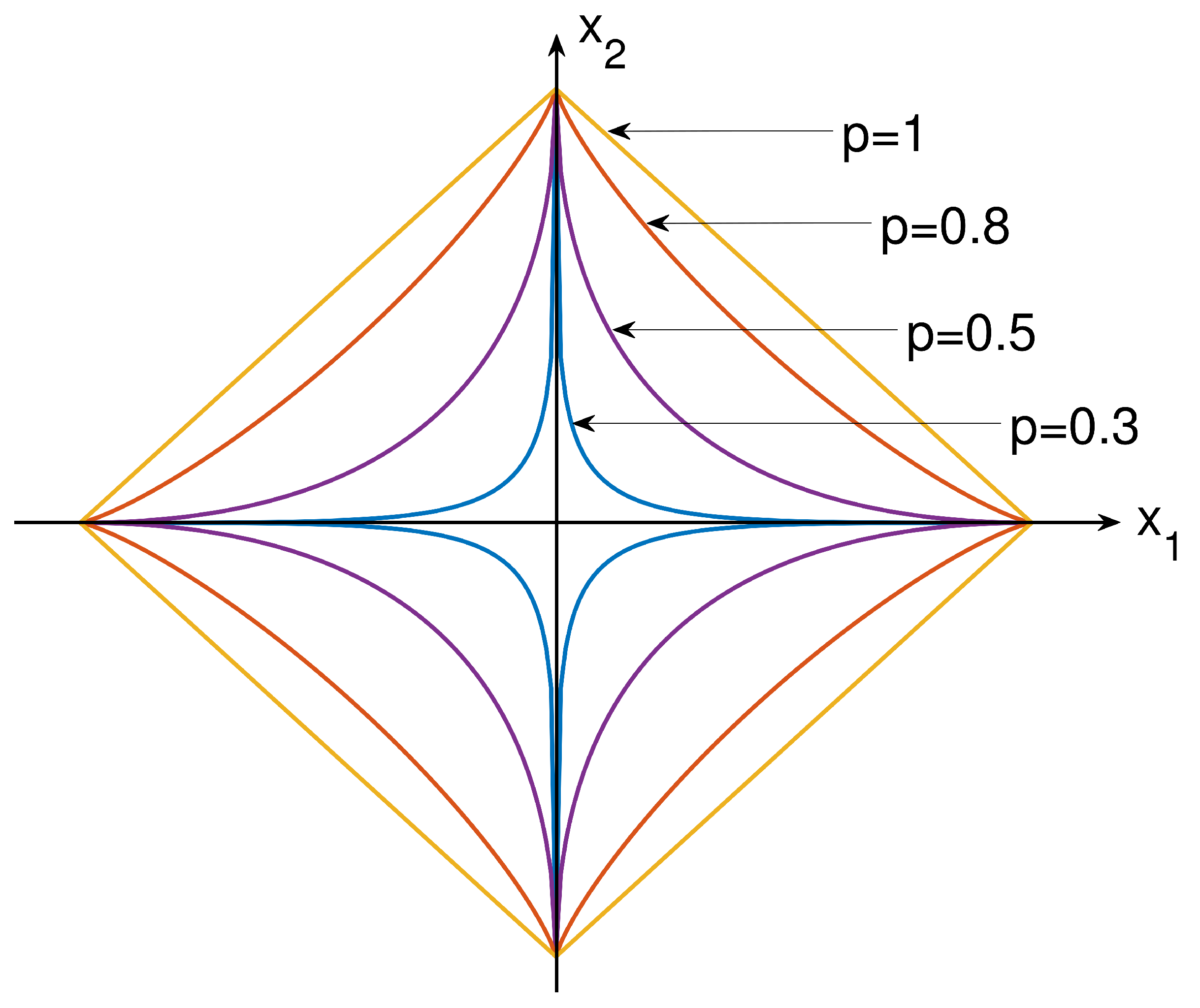
The ability to estimate the DOAs of two closely spaced sources is always an important indicator of the DOA estimation algorithm. Figure 2 is a norm ball of ${\mathbb{R}}^2$ space. The curves show that, the lower the p value, the easier it is to find a sparser solution. When faced with closely spaced sources, ${\ell }_p$ norm optimization has a greater possibility of obtaining a sparse solution, thereby, distinguishing two sources.

Figure 2. Unit norm ball.

As stated in the RIP condition, the uniqueness solution can be characterized in terms of the ${\delta }_K$ of matrix $\mathbf{A}$. Recall the smallest constants $0<{\delta }_K\le 1$ for which the matrix $\mathbf{A}$ satisfies the RIP of order K, that is

$$\left(1-{\delta }_K\right){∥\mathbf{x}∥}_2^2\le {∥\mathbf{Ax}∥}_2^2\le \left(1+{\delta }_K\right){∥\mathbf{x}∥}_2^2$$

(18)

It is clear that any K-sparse vector $\mathbf{x}$ is recovered via the ${\ell }_0$ norm minimization if and only if the strict inequality ${\delta }_{2K}<1$ holds. Define a new parameter to represent the RIP condition of matrix $\mathbf{A}$

$${\gamma }_{2K}=\frac{{\left(1+{\delta }_{2K}\right)}^2}{{\left(1-{\delta }_{2K}\right)}^2}\ge 1$$

(19)

The quantity ${\gamma }_{2K}$ can be made arbitrarily close to 1 by when the $\mathbf{A}$ is orthogonal column by column. As stated in [12], given $0<p\le 1$, if (20) for some integer $t\ge K$, then every K-sparse vector is exactly recovered by solving the ${\ell }_P$ norm minimization.

$${\gamma }_{2t}-1<4\left(\sqrt{2}-1\right){\left(\frac{t}{K}\right)}^{1/p-1/2}$$

(20)

When $t=K+1$, condition (20) becomes

$${\gamma }_{2K+2}<1+4\left(\sqrt{2}-1\right){\left(1+\frac{1}{K}\right)}^{1/p-1/2}$$

(21)

From (21), when $p\to 0$, the right side of the inequality becomes $+\infty$, which means the RIP condition number ${\delta }_{2K+2}\to 1$. That is to say, the smaller the value of p, the lower the ’approximate orthogonal’ requirement of sparse reconstruction for matrix $\mathbf{A}$. From the perspective of DOA estimation, as long as p is small enough, the ability of the algorithm to overcome the high correlation between adjacent columns in over-complete basis $\mathbf{A}$ is stronger, and the ability of separating spatial closely sources is stronger.

When $p\to 0$ the penalty of ${\ell }_p$ norm is close to ${\ell }_0$ norm. However, too small p may lead the algorithm to converge to a local optimization. The common ${\ell }_p$ norm optimization algorithms, such as FOCUSS usually choose $p=0.8$ based on experience [13]. In order to make p sensitive to the spectrum convergence and find a sparser solution, this section defines a decreasing processing of p by variation of the spectrum until $p<0.1$.

$$p^{(k+1)}=p^{\left(k\right)}-v^{\left(k\right)}$$

(22)

where $v^{\left(k\right)}={\parallel {\mathbf{X}}^{\left(k+1\right)}-{\mathbf{X}}^{\left(k\right)}\parallel }_F^2/{\parallel {\mathbf{X}}^{\left(k+1\right)}\parallel }_F^2$. When $v^{\left(k\right)}>p^{\left(k\right)}$, proves that the spectrum variation of this iteration is too large, then we directly reduce the p value to half of the previous time. Thus, the stopping criteria of the proposed algorithm is $v^{\left(k\right)}<\delta$, and $\delta >0$ is a small constant.

2.3. Adaptive Regularization Parameter Adjustment

According to (5), the regularization parameter $\lambda$ has a significant influence on the optimization process. However, balancing the relationship between residuals and sparsity is a difficult problem. At present, the methods for selecting regularization parameters include Generalized Cross Validation (GCV) [14], L-curve [15] etc. However, the above methods usually require massive data for prior computation and are, thus, not suitable for real-time DOA estimation. Another computational algorithm L1-SRACV [16], which considers the covariance matrix distribution, can also avoid the regularization parameters.

This section will provide a practical procedure for adjusting $\lambda$ in iteration. This method balances residuals and sparsity adaptively without massive prior simulation and working in the iteration process.

The covariance matrix of receiving data:

$$\mathbf{R}=\mathbf{Y}{\mathbf{Y}}^H/L$$

(23)

The ascending sorted eigenvalues $\gamma =\left[{\gamma }_1,{\gamma }_2,\cdots ,{\gamma }_M\right]$ can be obtained by eigenvalue decomposition of R. Therefore, the expected value of the noise energy $P_N$ is:

$$P_N=\frac{M{\sum }_{i=1}^{M-K}{\gamma }_i}{\left(M-K\right)L}$$

(24)

If source number K is unknown, there are two alternative methods. Under a low-SNR scenario, $P_N$ can be expressed by the minimal eigenvalue $P_N=\frac{M{\gamma }_{min}}{L}$. Under a high-SNR scenario, the source number K can be roughly estimated by the slope mutation of $\gamma$.

In a convergent and stationary iterative process with accurate estimation results, the power of residual $P_R={\parallel {\mathbf{T}}_1\parallel }_F^2={\parallel \mathbf{Y}-\mathbf{AX}\parallel }_F^2$ must converge to the noise power. Therefore, $P_R$ can be the measurement indicator of proposed algorithm, which should be controlled within a certain range. Considering the calculation error of $P_N$ and residual, the range of $P_R$ is determined to be $\left[0.75P_N,1.25P_N\right]$ after many simulation experiments.

The details are: in the kth iteration, if $P_R>1.25P_N$, this indicates an overemphasis on the influence of sparsity on the optimal value—the model is poorly fitting—thus, we reduce $\lambda$. If $P_R<0.75P_N$, this indicates an overemphasis on the influence of noise—the model is over fitting—thus we enlarge $\lambda$. If $0.75P_N<P_R<1.25P_N$, the descent direction works well, and nothing has to change. When the support set of the spectrum is determined, $P_R$ will not have obvious fluctuations, which indicates the convergence of this computation.

Proper initialization can considerably reduce the running time of the quasi-Newton method, and it has a much lower possibility to become trapped in a local minimum. The product of the dictionary and receiving data can be the initialization

$${\mathbf{X}}^{\left(1\right)}={\mathbf{A}}^H\mathbf{Y}$$

(25)

The proposed Algorithm 1 is described as follows.

Algorithm 1 The improved ${\ell }_p$ norm DOA estimator with adaptive regularization parameter adjustment.

1: Input:$\mathbf{A}$,$\mathbf{Y}$ 2: Initial: ${\mathbf{X}}^{\left(1\right)}={\mathbf{A}}^H\mathbf{Y}$, $p^{\left(1\right)}=1$, $ϵ={10}^{-6}$, $\delta ={10}^{-6}$, $P_N$, ${\lambda }^{\left(1\right)}=1$ 3: repeat 4:    Calculate ${\mathbf{T}}_{1\sim 4}^{\left(k\right)}$, update    ${\mathbf{X}}^{\left(k+1\right)}={\mathbf{X}}^{\left(k\right)}-{\mathbf{N}}_d^{\left(k\right)}$    ${\mathbf{N}}_d^{\left(k\right)}=\left({\mathbf{T}}_4^{\left(k\right)}-{\mathbf{T}}_3^{\left(k\right)}{\mathbf{T}}_4^{\left(k\right)}-{\mathbf{T}}_2^{\left(k\right)}{\mathbf{T}}_1^{\left(k\right)}+{\mathbf{T}}_3^{\left(k\right)}{\mathbf{T}}_2^{\left(k\right)}{\mathbf{T}}_1^{\left(k\right)}\right)$ 5:    Calculate $v^{\left(k\right)}={\parallel {\mathbf{X}}^{\left(k+1\right)}-{\mathbf{X}}^{\left(k\right)}\parallel }_F^2/{\parallel {\mathbf{X}}^{\left(k+1\right)}\parallel }_F^2$ 6:    if $P_R^{\left(k\right)}>1.25P_N$, then ${\lambda }^{(k+1)}=0.7{\lambda }^{\left(k\right)}$    else if $0.75P_N<P_R^{\left(k\right)}<1.25P_N$, then ${\lambda }^{(k+1)}={\lambda }^{\left(k\right)}$    else ${\lambda }^{(k+1)}=1.5{\lambda }^{\left(k\right)}$    end 7:    if $p^{\left(k\right)}>0.1$       if $v^{\left(k\right)}\ge p^{\left(k\right)}$, then $p^{(k+1)}=p^{\left(k\right)}/2$, go to 4       else $p^{(k+1)}=p^{\left(k\right)}-v^{\left(k\right)}$, go to 4       end    else $p^{(k+1)}=p^{\left(k\right)}$, go to 4    end 8: until$v^{\left(k\right)}<\delta$ 9: Output: reconstruct spectrum $\mathbf{X}$

2.4. Weighted Method

The weighted algorithm adds a weight in front of the spatial spectrum, which is a simple strategy to accelerate convergence and obtain higher resolution.

$$F\left(\mathbf{X}\right)\approx F_{ϵ}\left(\mathbf{X}\right)={\parallel \mathbf{Y}-\mathbf{AX}\parallel }_F^2+\lambda \sum _{i=1}^N{\left(w_i\sum _{j=1}^L{\left|X_{i,j}\right|}^2+ϵ\right)}^{\frac{p}{2}}$$

(26)

Set a small weight in the place where the signal may occur, and set a large weight in the place where there is no signal so that the small value of the spatial spectrum is smaller, the large value is larger and the overall solution is more sparse. Normally, the spatial spectrum of CAPON algorithm is used as the weight.

$$w_i=\frac{1}{a{\left({\theta }_i\right)}^H{\mathbf{R}}^{-1}a\left({\theta }_i\right)},i=1,\cdots ,N$$

(27)

The weighted method can not only accelerate the iteration but also improve the accuracy of the algorithm. Although the weighted method will increase the computational complexity, it can improve the estimated success rate even in worse situations.

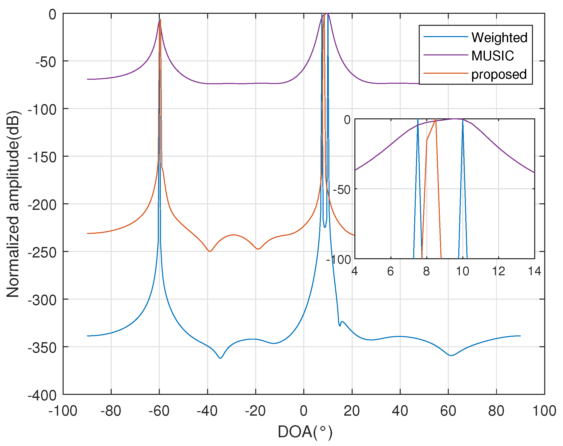
In Figure 3, the simulation is based on a eight-sensor uniform linear array with half-wavelength sensor spacing. The results show that the weighted method can distinguish two sources separated only by 3° with 200 snapshots and $\mathrm{SNR}=5\mathrm{dB}$.

Figure 3. The spectrum of distinguishing closely spaced sources by the weighted method.

3. Experimental Results

In this section, the empirical performance of the proposed algorithm is investigated and compared with those of MUSIC, FOCUSS and L1-SVD (${\ell }_1$ norm optimization by CVX toolbox [17]). The simulations are based on a 12-sensor uniform linear array with half-wavelength sensor spacing. All methods here use a grid of 1801 points in the range of $\left[-90°,90°\right]$, which means $0.1°$.

Considering the stability and good performance of all algorithms, the regularization parameter $\lambda$ of FOCUSS and L1-SVD was selected by the empirical value and $p=0.8$ for the FOCUSS algorithm. For the proposed method, we used adaptive $\lambda$ and p. The signal waveform was modeled as a complex circular Gaussian random variable $\mathbf{S}\left(t\right)\sim {\mathcal{N}}_C\left({\mathbf{0}}_M,{\mathbf{1}}_M\right)$. The variance of Gaussian white noise $\mathbf{N}\left(t\right)$ is determined by the SNR. According to $\mathbf{X}\left(t\right)={\mathbf{A}}_s\mathbf{S}\left(t\right)+\mathbf{N}\left(t\right)$, sensor data modeled as random variable $\mathbf{X}\left(t\right)\sim {\mathcal{N}}_C\left({\mathbf{0}}_M,\mathbb{E}\left\{\mathbf{X}\left(t\right){\mathbf{X}}^H\left(t\right)\right\}\right)$.

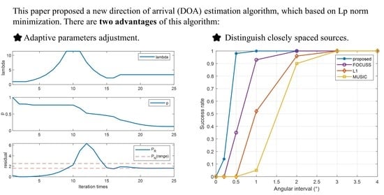
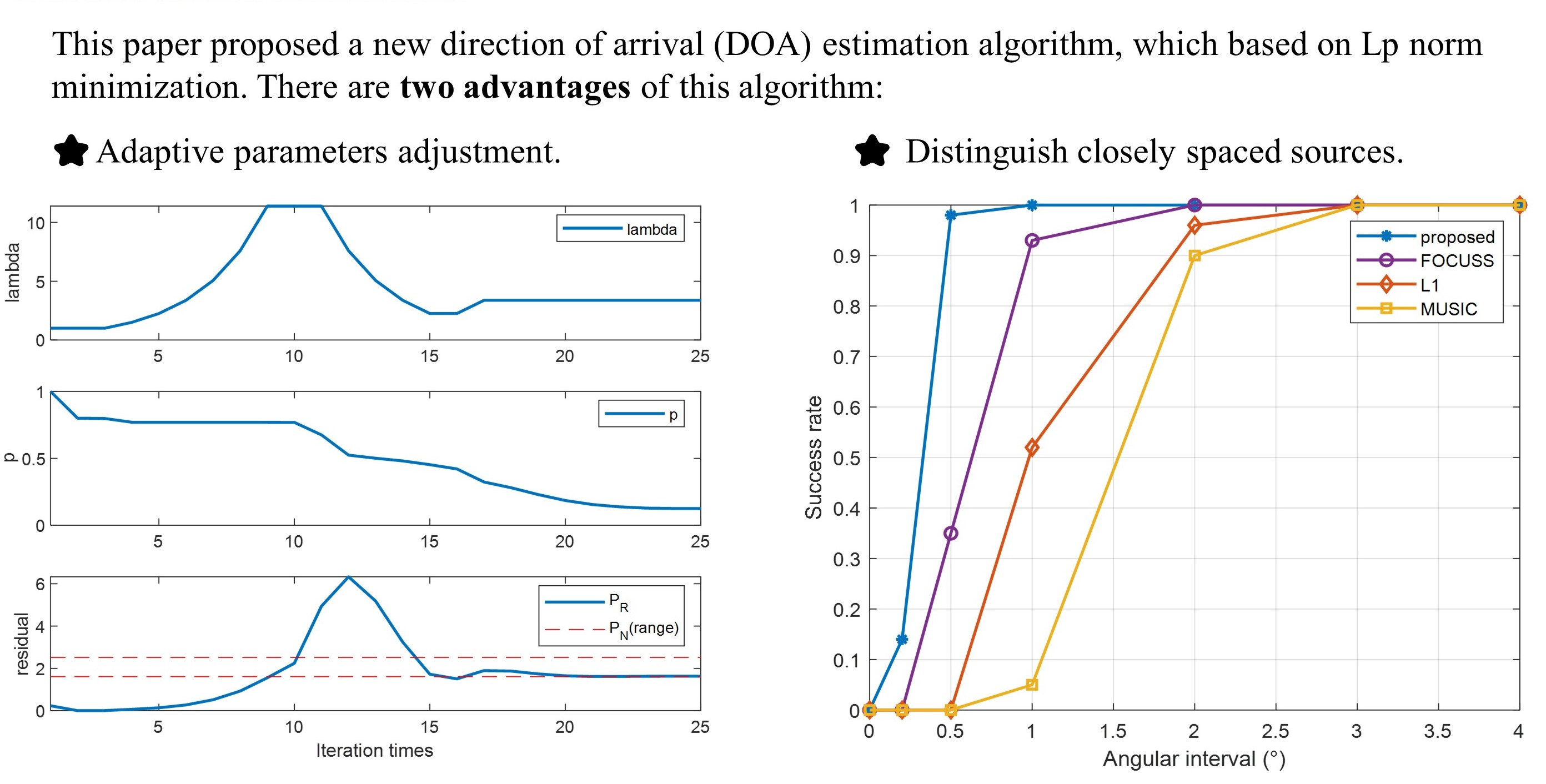
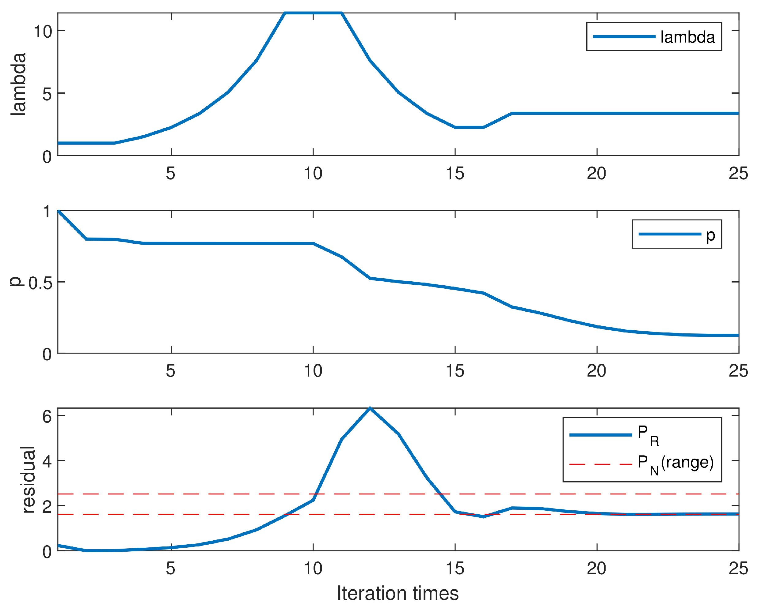
First, the highlight of the proposed algorithm is adaptive adjustment of parameters in the iterative process. The proposed algorithm automatically adjusts $\lambda$ according to the expectation power of residual $P_R$ and adjusts p according to the variation of spatial spectrum as shown in Figure 4 with $\mathrm{SNR}=0\mathrm{dB}$. The top subplot shows the variation of $\lambda$, the middle subplot shows the variation of p, and the bottom subplot indicates the convergence procedure of the residual.

Figure 4. The change of the $\lambda$, p and residual in the iteration process.

In Figure 4, we examine how the proposed method can adjust $\lambda$ and p to provide a convergence result. From the beginning, the result is too close to the least squares solution, which usually has a small residual. In order to obtain a sparser solution, $\lambda$ is increased to emphasize the importance of sparsity in iterations. For the whole process, the adaptive method maintains the residuals within expectations as much as possible until iteration convergence.

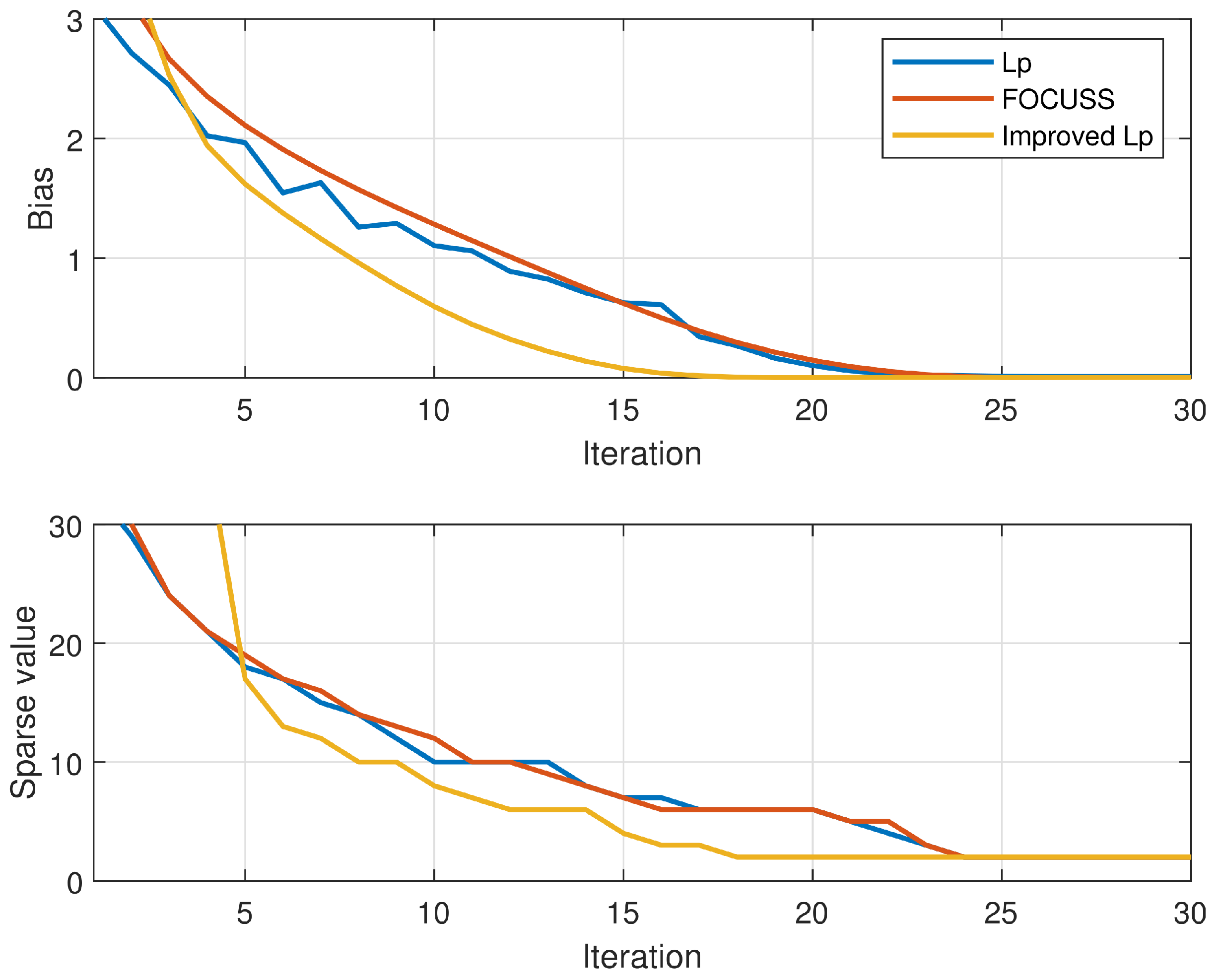
The adaptive methods can not only reduce the influence of the artificial selection of parameters on the results but also speed up the algorithm convergence to a certain extent. The convergence speed of the proposed algorithm was improved under the combined effect of acceleration strategy and adaptive methods. Figure 5 shows that the improved ${\ell }_p$ method will converge before 18 iterations, and the original method of ${\ell }_p$ and the FOCUSS algorithm requires nearly 24 iterations to converge.

Figure 5. The change of the spectrum bias and sparsity in the iteration process.

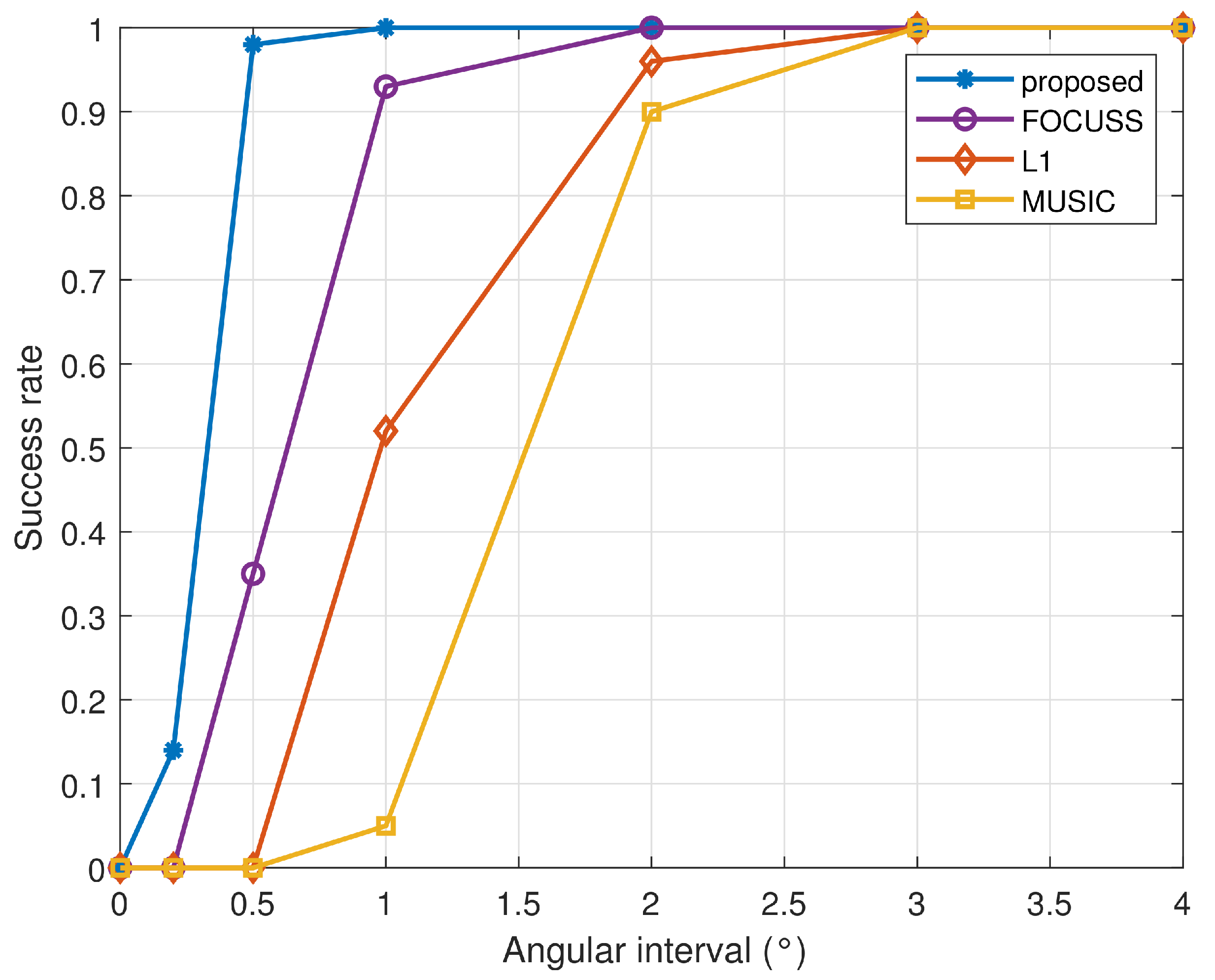
Assume two equal-power uncorrelated signals arrive from 0° and $0°+\Delta \theta$, respectively, where $\Delta \theta$ is varied from $0.1°$ to 4°. The SNR is set to 0 dB, and the number of snapshots is 200. The statistical result obtained via 200 multi-snapshot trials is shown in Figure 6 with the correct rate versus angular separation. As is clear from the figure, the proposed algorithm had a better ability to distinguish two closely spaced signals.

Figure 6. The probability of separating two closely spaced sources as a function of the angular interval.

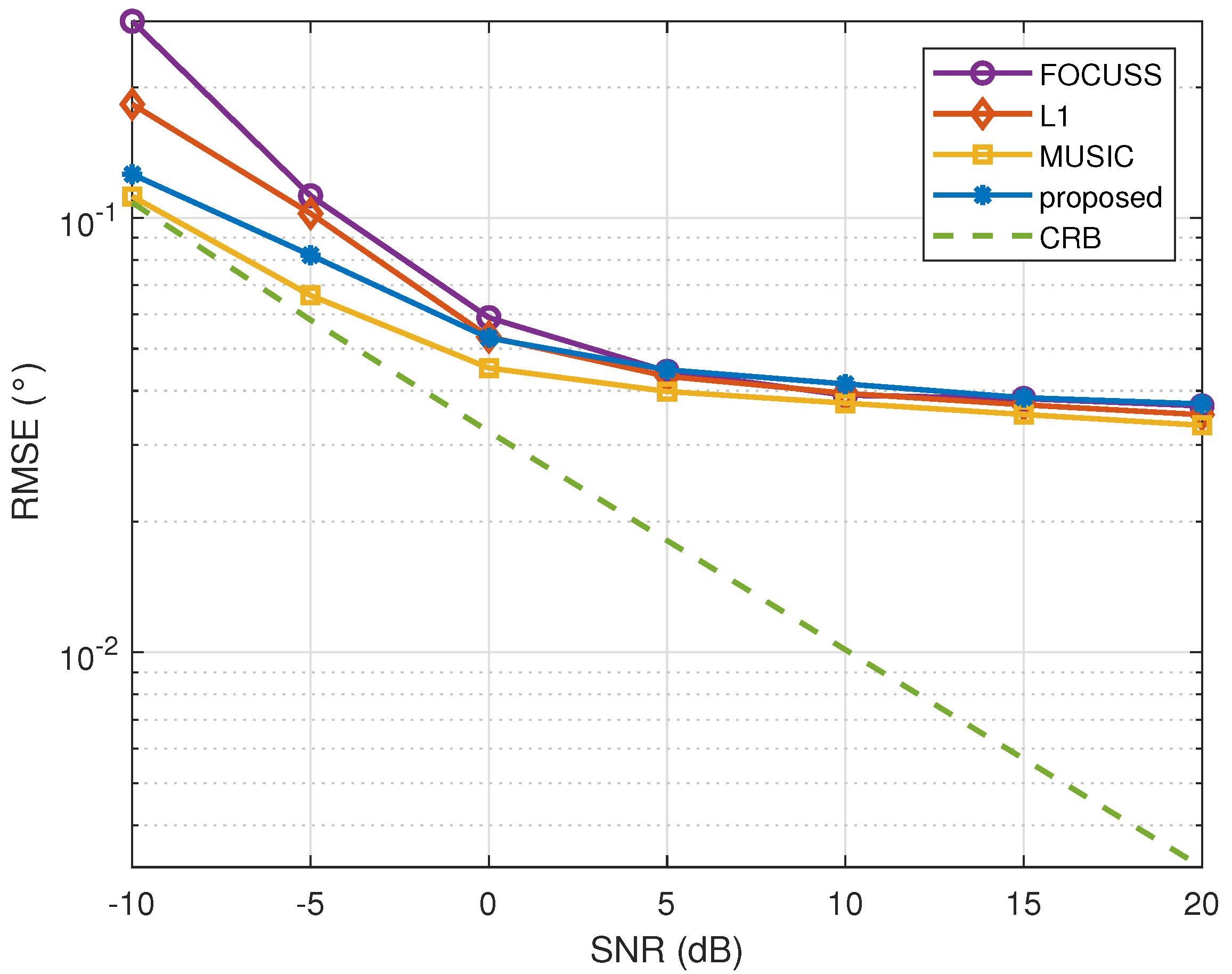
The bias curves in Figure 7 were obtained via 200 independent trials. Every multi-snapshots trial had a different DOA, ${\theta }_1$ and ${\theta }_2$, drawn within the intervals $\left[-11°,-9°\right]$ and $\left[19°,21°\right]$, and the snapshot number was 200. The root mean square error (RMSE) curves for different SNRs show that the resolution of the proposed algorithm meets the existing sparse reconstruction algorithm standards. Since the set grid size is $0.1°$, when the SNR is high, the resolution of these algorithms is limited by the grid, and the curves will gradually become flat.

Figure 7. The RMSE of the DOA estimates as a function of the SNR.

In conventional DOA estimation, this degree of error can generally be regarded as a correct estimation. The RMSE of the algorithm does not fully reflect the ability of DOA estimation. Sometimes, it is more meaningful to distinguish two sources in a certain spatial range with low resolution than to obtain only one estimation result with high resolution, which means that the latter option loses a target.

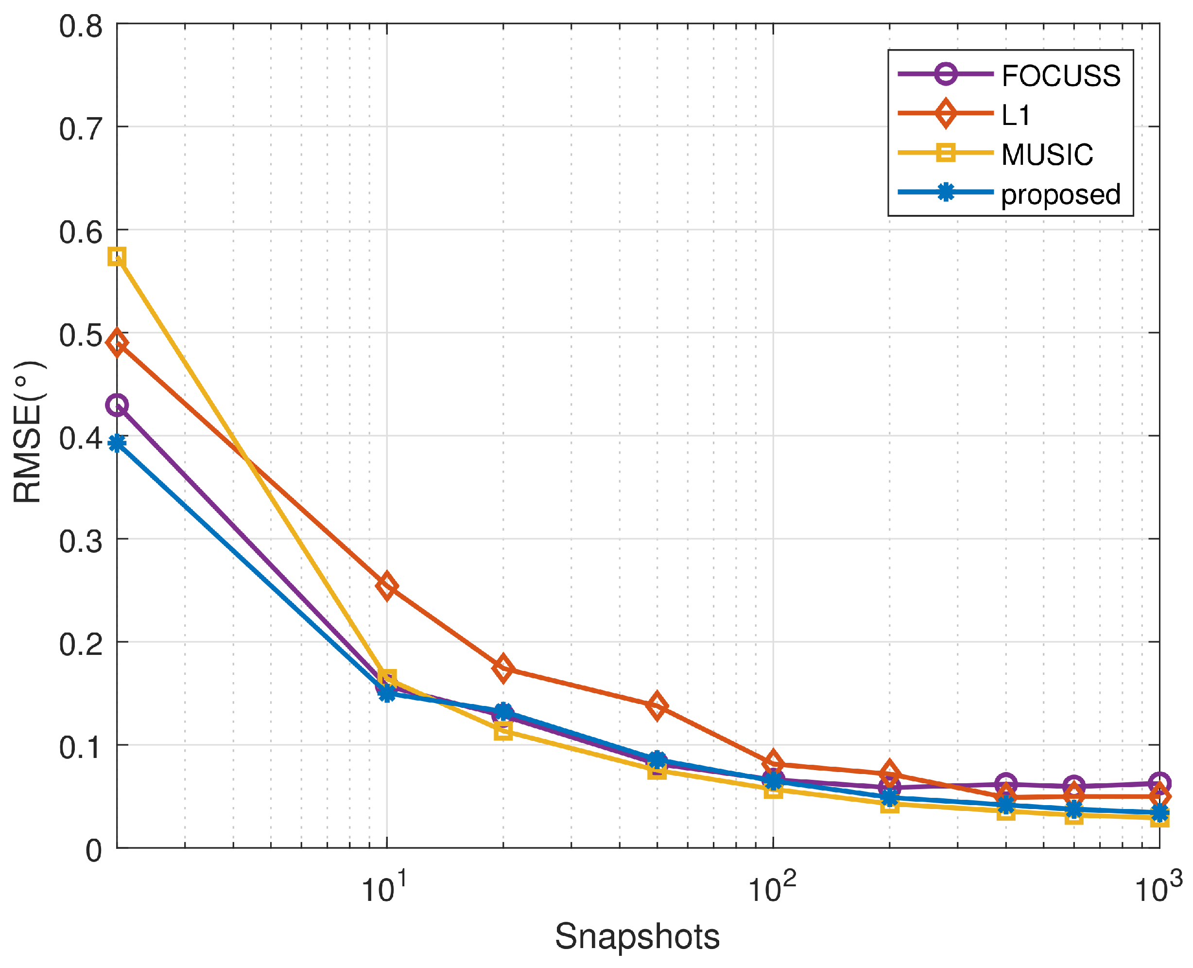
This section will close by examining the impact of the size of the data snapshot on the error-suppression criterion of the adaptive method. Consider two uncorrelated signals arriving from $\left[-11°,-9°\right]$ and $\left[19°,21°\right]$, where the SNR is fixed at 0 dB, the number of data snapshots is varied from 2 to 1000, and the remaining conditions are identical to those above. Figure 8 shows that, compared to the other methods, the proposed algorithm is stable in small and large snapshots.

Figure 8. The RMSE of the DOA estimates as a function of the snapshots.

As the focus of this paper is to improve the ability of the algorithm to distinguish closely spaced sources, the proposed algorithm and the conventional sparse reconstruction algorithms are essentially maintained in terms of the RMSE.

4. Conclusions

In this paper, an improved ${\ell }_p$ norm minimization DOA estimation algorithm was proposed. The proposed algorithm has two advantages: one is the greater ability to separate two closely spaced sources, and the other is the adaptive regularization parameter adjustment. The latter can reduce the impact of manual selection of $\lambda$ on the results and can accelerate convergence. The main motivation of this work comes from the desire to increase the practicability of sparse reconstruction algorithms.

By applying ${\ell }_p$ norm minimization with the quasi-Newton method and acceleration strategies, the proposed algorithm was faster than L1-SVD, the convex optimization algorithm. In addition, the adaptive method of the regularization parameter can run stably in most non-extreme situations. Compared to other seriously time-consuming methods or by optimizing the inequality-constrained minimization problem directly, the proposed method is more practical.