Abstract
An efficient physical optics (PO) calculation method is proposed for the electromagnetic (EM) scattering of electrically large targets coated with magnetized plasma characterized by asymmetric tensor dielectric parameters. The outer surface of the arbitrarily shaped target is discretized into triangular elements. According to the principle of tangent plane approximation and by using the plane wave spectrum expansion method, the scattered field from one triangular element is derived as a double integral in the spectral domain. To obtain the solution in the spatial domain, the saddle point method is used to asymptotically calculate the integral. Then, the equivalent surface currents (ESCs) are constructed by calculating the surface field at the outer surface of the planar model, from which the PO solution is derived by using the Stratton–Chu integral. Moreover, to interpret the field propagation process in the plasma layer quantitatively, the total scattered field of the coated planar model is decomposed into the superposition of different mode field components. It is observed that the scattered fields demonstrate an inherent cross-polarization phenomenon due to the nonreciprocal constitutive relation of the plasma, which is a distinct feature and is different from the general anisotropic medium whose dielectric parameters can be diagonalized. The effectiveness of the proposed method is verified by numerical results. Furthermore, the proposed algorithm consumes less calculation time and memory as compared to commercial full solvers.
1. Introduction
As we all know, plasma is the fourth state of matter formed by gas ionization. Since the first discovery [1], due to the unique propagation characteristics of EM waves in plasma [2,3,4,5,6], it has attracted great attention in many fields such as target stealth technology represented by scatterer radar cross-section (RCS) control, and radiation system design represented by an antenna or a radome [7,8,9,10]. The research on the propagation effects of ultra-high frequency EM waves and microwaves in plasma can be roughly divided into two categories. The first type is the impact of the plasma sheath on EM wave propagation during spacecraft reentry into the atmosphere. When high-speed aircraft reenter the atmosphere, a plasma sheath with a complex structure will be produced on the surface of the reentry body and the surrounding space. The sheath with different parameters has different effects on the absorption, refraction, and reflection of the incident EM wave. When the attenuation of EM wave power is serious, it will cause signal interruption; that is, the so-called “black barrier” problem. It will also seriously affect radar detection and identification of reentry targets. The other is to generate plasma with controllable parameters through artificial means, including high-voltage ionization, isotope injection, etc. The research community has great expectations for the development and application of artificial manufacturing plasma technology. This paper is mainly based on the expected research on the high-frequency theoretical calculation method of EM wave scattering of plasma-coated targets.
In the existing research on the theoretical calculation method of EM scattering for plasma-coated targets, most of the plasma objects with complex flow field properties are simplified into non-flow field plasma layers, and the simplified plasma coating target is closer to the artificially manufactured plasma layer coating model. The research on the theoretical calculation method of EM scattering of plasma-coated targets can be roughly divided into three categories. One is the rigorous analytical method research carried out on the scattering of ideal-shape target models, such as plasma-coated cylinders and spheres [11,12,13]; The second category is the study of numerical calculation methods for EM scattering of plasma-coated targets with finite electric size and arbitrary shapes [14,15,16,17,18], and also includes research on numerical calculation method improvement or acceleration [19,20,21]. However, as the frequency of EM waves increases and the complexity of plasma material parameters increases, numerical calculation methods are facing a sharp increase in calculation time and memory requirements. The third category is the study of high-frequency calculation methods represented by the physical optics (PO) method [22,23,24,25,26,27]. Reference [22] calculated the monostatic RCS of the electrically large target simulated by the non-uniform rational B-spline (NURBS) surface covered by non-uniform and non-magnetized plasma. Yu [23] analyzed the scattering characteristics of hypervelocity models with shooting and bouncing rays (SBR). Liu [24] investigated the multi-band scattering characteristics of a blunt cone with a nonuniform plasma shroud by using the physical optics (PO) method. It should also be pointed out that the plasma model used in the above-mentioned high-frequency calculation method is not magnetized, and most models only use scalar media parameters to characterize plasma, instead of using an asymmetric tensor to characterize the plasma medium attributes. The propagation of EM waves by magnetized plasma usually shows anisotropic characteristics, and its dielectric parameters should be in the form of an asymmetric tensor [28,29] to characterize its non-reciprocal constitutive relationship. Only in this way can the inherent cross-polarization scattering phenomenon of magnetized plasma be reflected, which is similar to the cross-polarization scattering characteristics of the “surface” anisotropic medium. The asymmetric off-diagonal elements in the dielectric parameter tensor of plasma indicate that its constitutive relationship is more special than that of general anisotropic media, which makes the propagation process and mechanism of EM waves in the plasma layer more complicated. In our previous research, Yao [30,31] proposed an EM scattering estimation method for targets coated with anisotropic uniaxial and biaxial media based on the spectral domain method. In Yao’s method, the dielectric tensor of anisotropic media can still be diagonalized, and its scattering model is simpler than that of plasma coating.
Aiming at the targets coated with magnetized plasma characterized by asymmetric tensor dielectric parameters, this paper proposes an efficient and accurate physical optics algorithm based on a spectral-domain asymptotic calculation to achieve high-frequency scattering prediction of plasma-coated electrically large targets. The inherent cross-polarization scattering phenomenon of plasma is demonstrated in the research, and the mechanism of high-frequency scattering of EM waves propagating in the plasma layer is interpreted by analyzing different mode fields. The complex target surface of arbitrary shape is discretized into many triangular facets. Once the ESCs on the surface of the coating facet are obtained, the total scattering field can be obtained by superposing the corresponding integral formula. According to the tangent plane approximation principle of physical optics, the surface field of a coated facet is approximated as that of the infinite coated plane at the tangent plane. Therefore, firstly, it is necessary to solve the scattering field of the plasma-coated infinite PEC plate. In this paper, the spectral domain combined with saddle point evaluation (SDM-SPE) is applied to obtain the spectral-domain asymptotic solution of the scattering field of an infinite plasma-coated slab. To reveal the field propagation mechanism in the plasma layer, the total scattering field of the coated slab is further decomposed into the superposition of different mode field components, and the formation process of each mode field is quantitatively analyzed. The amplitude and phase of the main mode field and their effects on the total scattering field are discussed. Finally, the monostatic RCSs of canonical or complex targets coated with anisotropic plasmas are calculated. Compared with the numerical full-wave method, the proposed algorithm is more efficient and more suitable for the calculation of the scattering field of electrically large complex coated targets.
The remainder of this paper is organized as follows. In the second section, the plane spectral expansion method is first used to obtain the strict spectral-domain solution for the scattering of an infinite plasma-coated plate by plasma. Furthermore, the scattering total field is decomposed into the superposition of the secondary scattering fields of different modes, and the field components of each mode and the transmission relationship between them are solved. Section 3 constructs the physical optics algorithm for the EM scattering of complex targets coated with magnetized plasma. Numerical examples are given to illustrate the effectiveness of the proposed method in Section 4, and the scattering characteristics of anisotropic plasma-coated planar models and complex targets are discussed and analyzed. Section 5 gives the conclusion.
2. The Scattered Fields for An Infinite Plasma-Coated PEC Slab
In this section, we will study the exact spectral-domain solution of the scattering problem of an infinite PEC plate coated with anisotropic plasma. Firstly, the expression of the plane wave spectrum in anisotropic plasma is derived, then the total field in the spectral-domain of the infinite coated plate is obtained by strict boundary condition constraints, and the ray field solution of the spatial EM field is obtained by using the saddle point method. Finally, to analyze the propagation mechanism of the EM wave inside and outside the plasma layer, we decompose the total scattering field into the superposition of secondary scattering fields of different modes and solve the respective mode fields and the transmission relations between them.
2.1. The Plane Wave Spectrum Representation of the Field in the Plasmas
The Maxwell equation in the anisotropic magnetized plasmas can be expressed as
The permittivity and permeability tensors of the plasma layer are characterized by two matrices:
Here, , and are the complex function of electron plasma frequency, wave frequency, electron-neutral collision frequency, and electron cyclotron frequency. Their exact expressions are present in the previously published literature [32].
The Fourier expansions of the EM fields in Equation (1) are defined as
where , . From Equation (1), the formulas of each partial wave in Equation (3) satisfy
It can be derived by Equation (4) that
The existence of in Equation (5) can derive
where . If are determined, Equation (6) has four roots and ; that is,
Thereby type I and II waves propagate in different directions . Substitution of or into Equation (4) leads to
or
where
Equations (8) and (9) represent the type I and II waves in plasmas, and the parameters determine their complex amplitudes. Especially, type I and II waves with propagate along axes, which are
2.2. The Total Scattered Fields in the Spectral Domain
Consider the planarly stratified model depicted in Figure 1, which shows an infinite PEC plate coated with a homogenous plasma layer whose thickness is . This is divided into two distinct regions; namely, Region 0 for outer free space and Region 1 for the inner anisotropic plasma layer. A set of Cartesian axes is adopted, with an axis normal to the surface of the plasma layer extending from the bottom interface () to the top interface ().
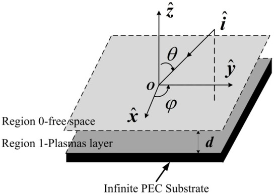
Figure 1.
The model of an infinite plasma-coated PEC slab.
The Fourier expansions of the EM fields in region 0 (air) and region 1 (plasmas layer) are
where , are the eigenvalues, and the subscripts 0, 1 denote the fields in the air and the plasma layers, respectively. Equation (12) indicates that the arbitrary EM fields can be expanded as plane waves with different eigenvalues in the spectral domain.
Taking the case of , the EM fields in region 1 (plasma layer) can be written as
Similarly, the EM fields in region 0 (air) can be represented as
In Equations (13) and (14), the subscripts indicate the partial EM waves propagating along and , respectively. Thereby, the components of the incident and scattered electric fields in Equation (14) (that is, ) are extracted as
where determine the complex amplitudes of the scattered fields, which are requested in our investigation. Meanwhile, correspond to the incident fields.
The boundary conditions at the top and bottom interfaces of the plasma slab can be derived as
Substituting Equations (13) and (14) into Equation (16), the requested are represented in terms of by suppressing ; that is
where the formulas of are
When , it can be obtained by a similar derivation:
The expression form of is the same as that of , only the following substitutions are needed: . So far, the scattered electric field in the spectral domain in Equation (15) can be established. The corresponding total spatial scattering field can be obtained by the following spectral-domain integration:
The saddle-point method is used to approximate the above double integral in Equation (19), and a high-efficiency spatial ray field calculation formula can be obtained, which is particularly suitable for the calculation of a fully propagating EM field. The saddle point can be obtained by derivation as
where are the angles of the field point. Equation (20) indicates that the saddle point represents the specular reflection point of the field point by the surface of the infinite coated plate. Thereby, the scattered field asymptotically derived by the saddle point evaluation can be reasonably regarded as the reflected field.
After setting the incident angle, the eigenvalue of the plane wave spectrum corresponding to the saddle point is
Therefore, the total scattered electric field of the coated plate in the spatial domain (that is, Equation (20)) can be written as
2.3. Propagation Analysis of Each Secondary Scattered Field
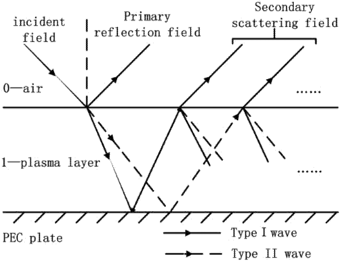
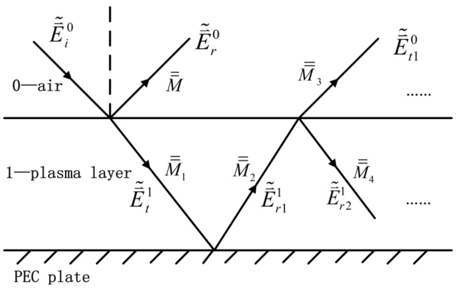
In the previous section, the strict spectral-domain solution of scattering from the anisotropic plasma-coated plane has been obtained, but the results cannot directly describe the physical process of the EM wave first penetrating the plasma, then multiple reflections in the layer and finally penetrating. In this section, we will use quantitative mathematical analysis to reveal the physical images of the propagation process of EM waves in each mode corresponding to different ray paths inside and outside the plasma layer. In this section, we will use quantitative mathematical analysis to reveal the physical images of the propagation process of EM waves in each mode corresponding to different ray paths inside and outside the plasma layer. The propagation process of EM waves incident on the plasma dielectric layer is shown in Figure 2. The total field on the upper surface of the dielectric layer includes the incident field, the primary reflection field formed by the incident wave on the upper surface of the plasma, and the superposition of each secondary scattering field transmitted to the dielectric layer, reflected in the layer and then transmitted to the air.

Figure 2.
The propagation model of an infinite plasma-coated PEC slab.
To deduce the field of the EM wave transmitted into the air through n reflections in the plasma layer, a series of coefficient matrices are introduced on each interface to establish the correlation between the EM wave in each mode and the incident wave, as shown in Figure 3. The specific correspondence is as follows:

Figure 3.
The transmission relationship of the electric field in the plasma layer.
- is the primary reflection field of the EM wave incident on the surface of the plasma, is the corresponding reflection matrix;
- is the initial transmission field of the EM wave incident into the plasma layer, is the corresponding transmission matrix;
- is the reflected field after the initial transmission field is incident on the bottom PEC boundary, is the reflection matrix formed by and ;
- is the transmission field transmitted into the air after one reflection in the layer, is the transmission matrix formed by and ;
- is the reflection field that is reflected back to the medium on the upper surface after one reflection in the layer, is the reflection matrix formed by and ;
The above-mentioned fields and the corresponding coefficient matrix are derived below;
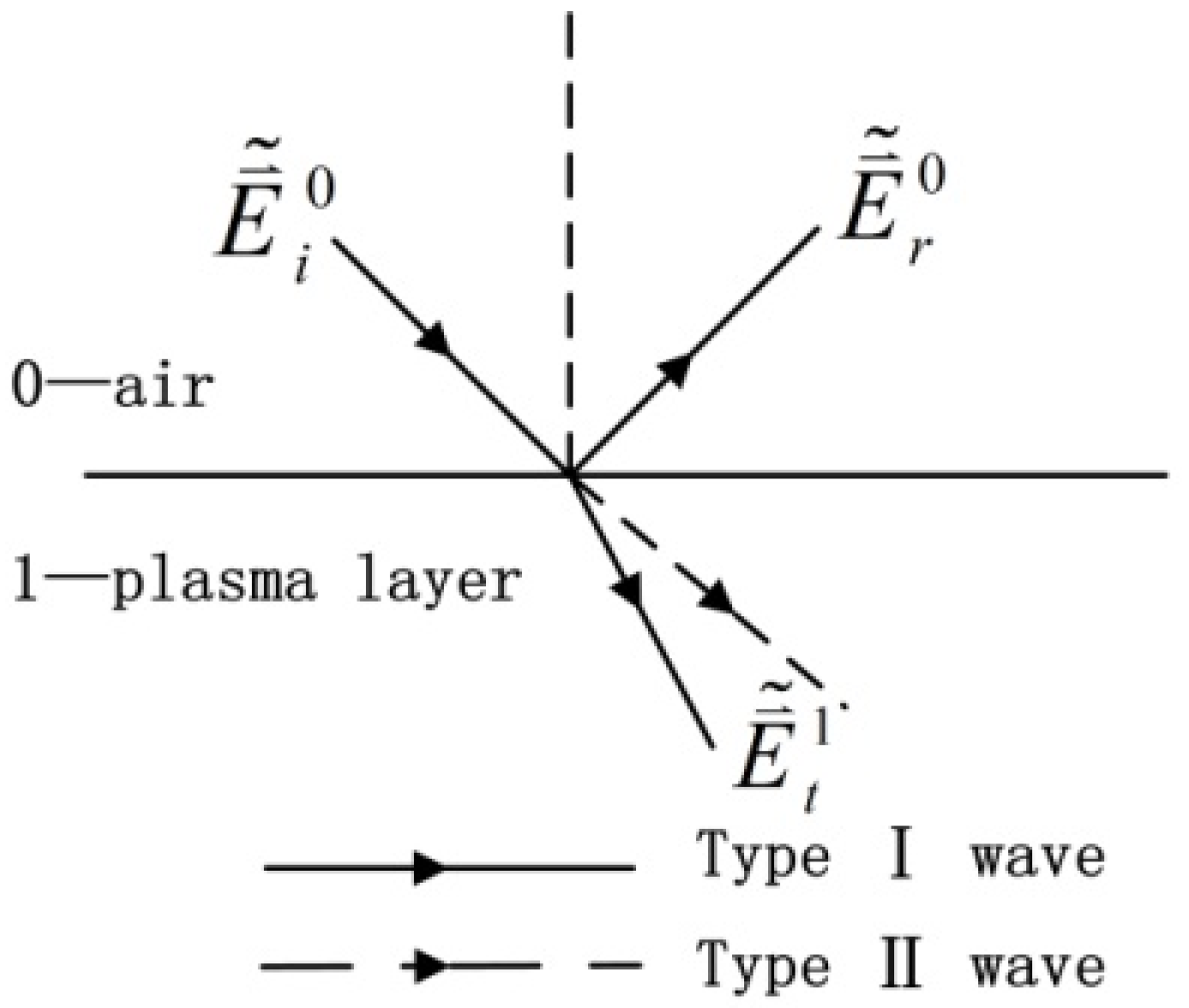
- The first reflection on the outer surface
When the EM wave is incident on the plasma layer and acts on the upper surface, as shown in Figure 4, the primary reflected wave does not enter the layer, and the problem can degenerate to a half-space problem: the upper half-space is air with incident field and primary reflection field ; the lower half-space is an anisotropic plasma layer with only the initial transmission field .

Figure 4.
Reflection and transmission of EM wave from air to the surface of the plasma layer.
In region 0, there are downward incident waves and upward primary reflected fields. The corresponding expressions of the EM field in a spectral domain are as follows:
where . In region 1, there is only a downward initial transmission field, and its expression in the spectral domain can be written as
The boundary conditions at the interfaces of the plasma layer can be derived as
It can be solved by Equation (26)
where
where
- 2.
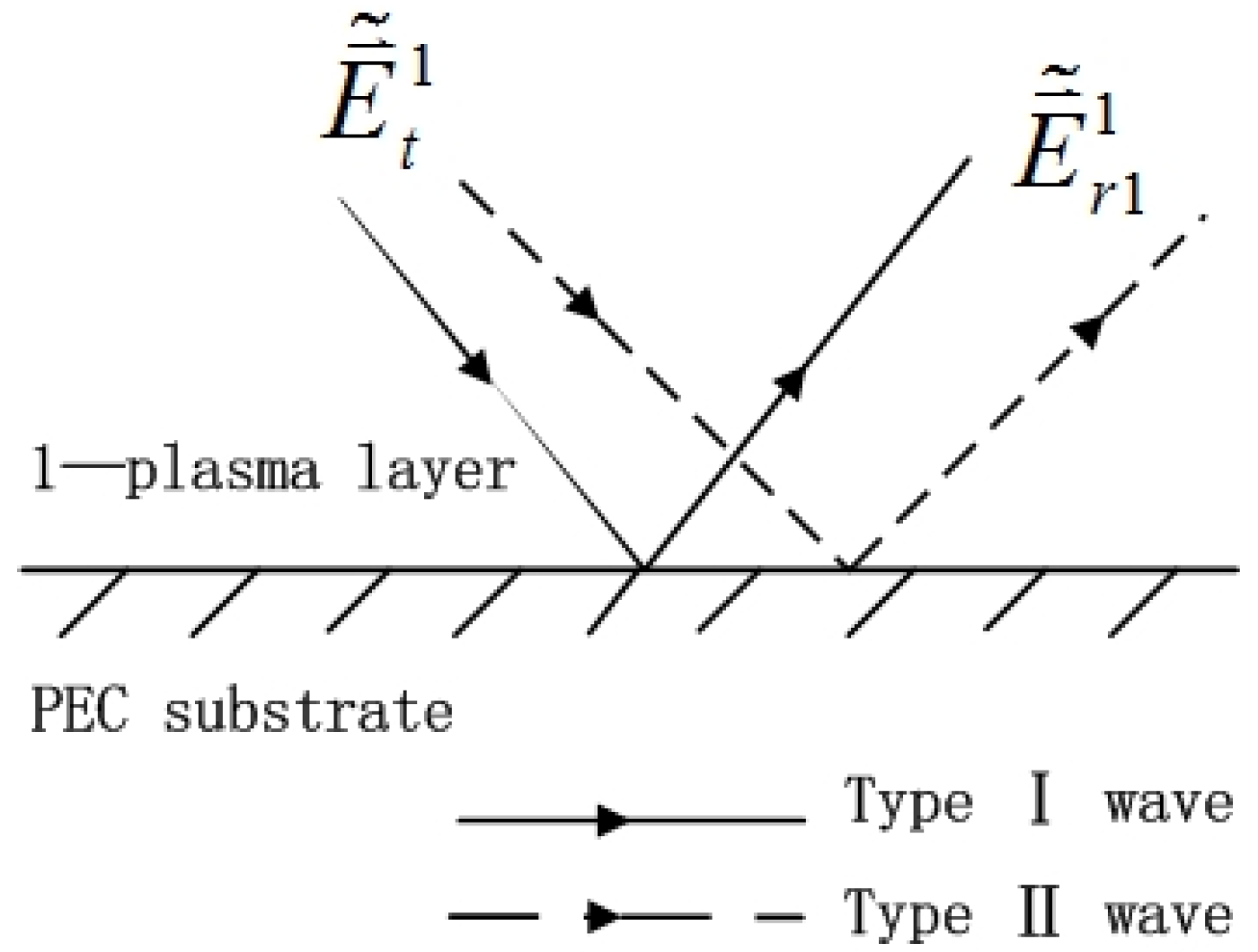
- The reflection of the substrate in the plasma layer
The original model can be simplified to the model of an anisotropic plasma half-space on the PEC substrate, as shown in Figure 5. At this time, there is the initial transmission field and its reflection field in the anisotropic half-space after the incidence on the PEC substrate; that is
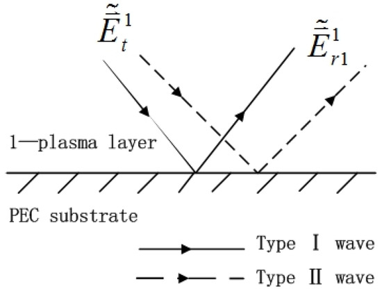
Figure 5.
Reflection of EM wave on PEC substrate.
The reflected field on the PEC substrate is
The boundary condition at the PEC substrate is
Similarly, it can be solved by Equation (32)
- 3.
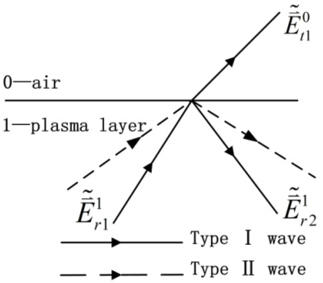
- Transmission from the plasma layer to the upper half-space
As shown in Figure 6, the upper half-space is air, and only the transmission field travels from the layer to the air. The lower half-space is an anisotropic plasma layer, with and its reflected field reflected on the upper surface of the plasma.
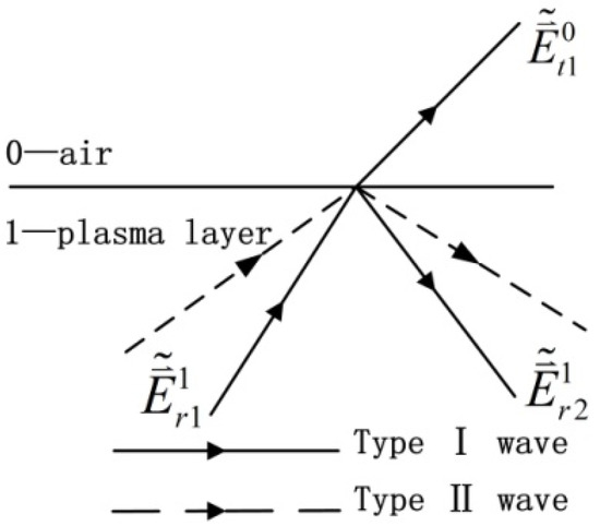
Figure 6.
Reflection and transmission of EM waves from plasma layer into the air.
In the plasma half-space, there are and its reflection field after reflection on the upper surface of the plasma; that is
where
In the upper half-space, the transmitted field that first penetrates the air after one reflection in the layer can be written as:
The boundary conditions at the interfaces of the plasma layer can be derived as
It can be derived by Equation (37) that
where
where . Then, the coefficient matrix of the EM wave transmitted into the air after one reflection in the layer can be written as
Using the expression of the transmission matrix, the coefficient matrix of an EM wave reflected n times in the layer and then transmitted to the air is
Then, the field transmitted into the air after n refractions in the layer can be expressed as
where .
Each secondary scattered field constitutes a proportional series, and the total secondary scattered field can be obtained by superimposing all the secondary scattered fields:
3. Physical Optical Solution of Electrically Large Plasma-Coated Targets
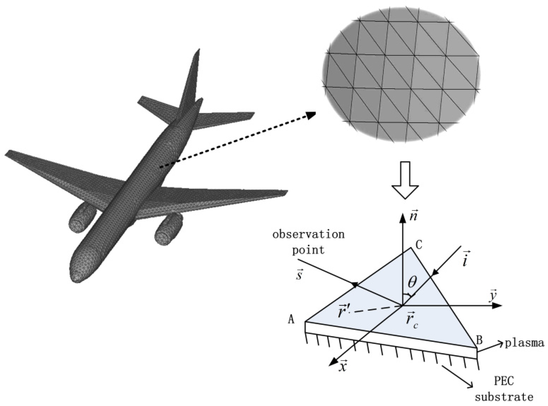
When estimating the scattering field of a complex target, flat elements are usually used to discretize the target surface. The physical optics algorithm discretizes the target surface into many flat triangular facets, calculates the scattering field of each illuminated flat triangular facet, and finally superimposes it to obtain the total scattering field of the target [33]. Figure 7 shows the discrete flat triangular facets on the outer surface of a coated aircraft. According to the principle of tangent plane approximation, it is considered that the surface EM field of the triangular facet has the same characteristics as the EM field on the infinite plane tangent to the surface at the incident point. Therefore, as long as the surface EM field of the plasma-coated infinite plate is obtained, the physical optics algorithm for the EM scattering of the plasma-coated target can be constructed.

Figure 7.
Model of the discrete complex target.
3.1. Surface EM Field of an Infinite Plasma-Coated PEC Slab
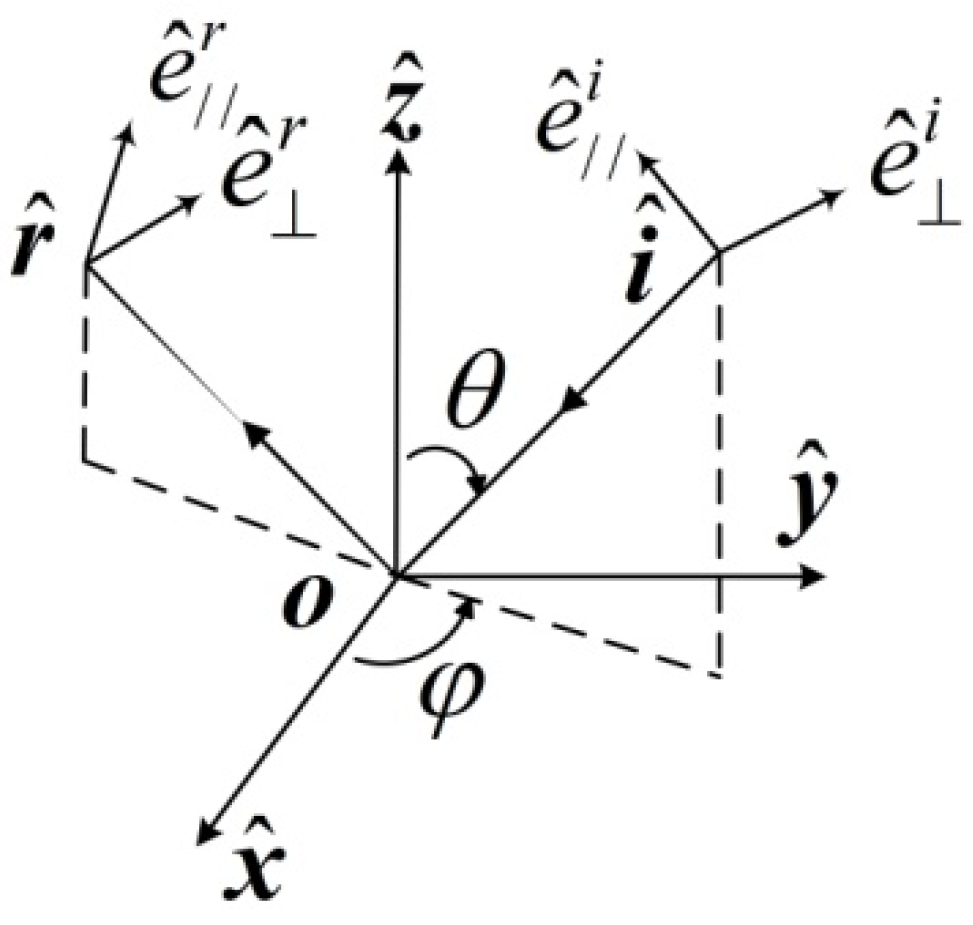
As shown in Figure 8, assuming the incident angle and the scattering angle are, respectively, , , then the incident direction and the reflection direction are .
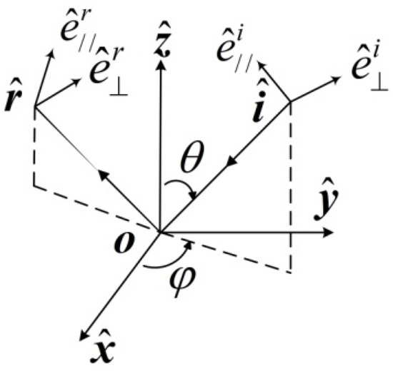
Figure 8.
The perpendicular and parallel vectors and .
From the previous section, after the saddle point of the total scattered field is calculated, the wave vector corresponding to the saddle point is .
For the surface EM field at , there are
where . Substituting Equations (15) and (44) into Equation (45), we can arrive at
Assuming Equation (46) becomes
The incident and reflected electric fields and their corresponding magnetic fields at the origin o are written as
where is the vector of the origin o. Assuming are the coefficients of the reflection matrix , which are defined as
we can arrive at
where the subscript denoting the eigenvalues of in Equation (50) are replaced by respectively. Replacing the vector in Equation (48) with the vector from the origin to the center of each triangular facet, the surface EM field at the center of each triangular facet can be obtained as
3.2. PO Solution of Plasma-Coated Targets
The equivalent EM current at the center of each triangular facet is
According to the Stratton–Chu formula and the far-field approximation condition, the scattered field contributed by the triangular facet can be obtained as
where is the vector corresponding to the field point. Using the Gordon integration method [34], the PO scattering electric field of the facet ABC can be derived as
where , are the direction vectors of the three vertices of the triangular facet. When the incident direction is perpendicular to the facet, namely , Equation (54) will be invalid, and the scattered electric field can be written as
where A is the area of the facet ABC.
At a certain incident angle, when triangular facets on the surface of a complex target are illuminated by the incident wave, the scattering field of each facet is , and the scattering field of the entire target under a high-frequency approximation is
4. Numerical Simulations and Discussion
Firstly, by comparing the reflection coefficient of the plasma-coated infinite plate obtained by the method in this paper with the results in the literature, the correctness of this method is verified, and the scattering characteristics of a plasma that is different from an ordinary uniaxial dielectric coating are analyzed. Then, the scattering characteristics of plasma coating are explored from the following two aspects.
Scattering characteristics of plasma-coated infinite PEC plate: the variation of the amplitude and phase of the scattered total field and the different mode fields after decomposition are investigated in detail when the parameters such as incident angle and coating thickness change.
Scattering characteristics of plasma-coated complex targets: the corresponding scattering characteristics of typical shapes and complex targets under different polarization incidences and different dielectric coatings are investigated, and their scattering contributions are analyzed.
4.1. Validation and Analysis
To verify the correctness of the asymptotic solution of the spectral domain in this paper, we first calculated the reflection coefficient of the plasma-coated infinite PEC plate and compared the result with the result calculated by the numerical difference algorithm in the literature [35]. The plasma relative permittivity tensor elements are, respectively, , and the incident angle is . Figure 9 shows the reflection coefficient of the plasma-coated infinite PEC plate when the incident angle and coating thickness change. Excellent agreements are obtained between the results from the two methods. Therefore, the asymptotic solution of the scattered field obtained by the spectral domain method is reasonable and reliable.
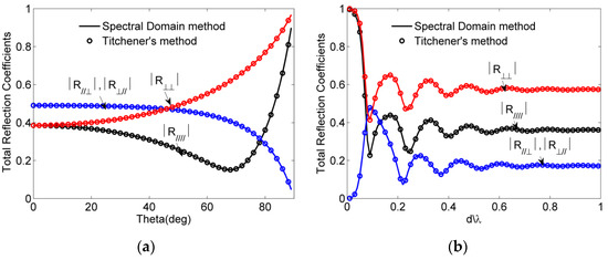
Figure 9.
The reflection coefficients of the plasma-coated slab with a PEC substrate: (a) against the angle incidence ; (b) against the slab’s thickness .
To further study the scattering characteristics of plasma and general anisotropic media, the reflection coefficients of two different uniaxial medium coatings will be calculated by using the method of reference [35], and the results are compared with those of a plasma coating. The general anisotropic uniaxial dielectric tensor is a symmetric matrix, which can be converted into a diagonal matrix by rotating the coordinate axis. Taking the following two uniaxial media, the diagonalized dielectric tensors at are
With the rotation of the angle , the dielectric tensor matrix of the uniaxial medium 1 will not change showing surface isotropy, while the dielectric tensors of uniaxial medium 2 are symmetric matrices at with off-diagonal elements; for example, at , the dielectric tensor is
The most remarkable characteristic of plasma is that its dielectric tensor matrix is asymmetric, and there are always opposite off-diagonal elements. Take the plasma dielectric tensor as
Figure 10 shows the reflection coefficients when the above plasma and uniaxial media are coated separately, and the reflection coefficients with uniaxial media coated are obtained by Titchener’s method. The coating thickness is .
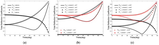
Figure 10.
Comparison of reflection coefficients of infinite PEC slab coated with different media: (a) plasma coating; (b) uniaxial media coating at ; (c) uniaxial media coating at .
In Figure 10a, the scattering of the plasma-coated infinite plate is independent of the angle and cross-polarization always exists. In Figure 10b, the dielectric tensors of the two uniaxial media are diagonal matrices at , and no cross-polarization is generated. In Figure 10c, the dielectric tensor of the uniaxial medium 2 is an off-diagonal matrix with off-diagonal elements at , and the phenomenon of cross-polarization has appeared. The unique dielectric tensor form of plasma makes it different from general anisotropic media and it has inherent cross-polarization scattering characteristics.
4.2. The Scattering Characteristics and Analysis of a Plasma-Coated Infinite PEC Plate
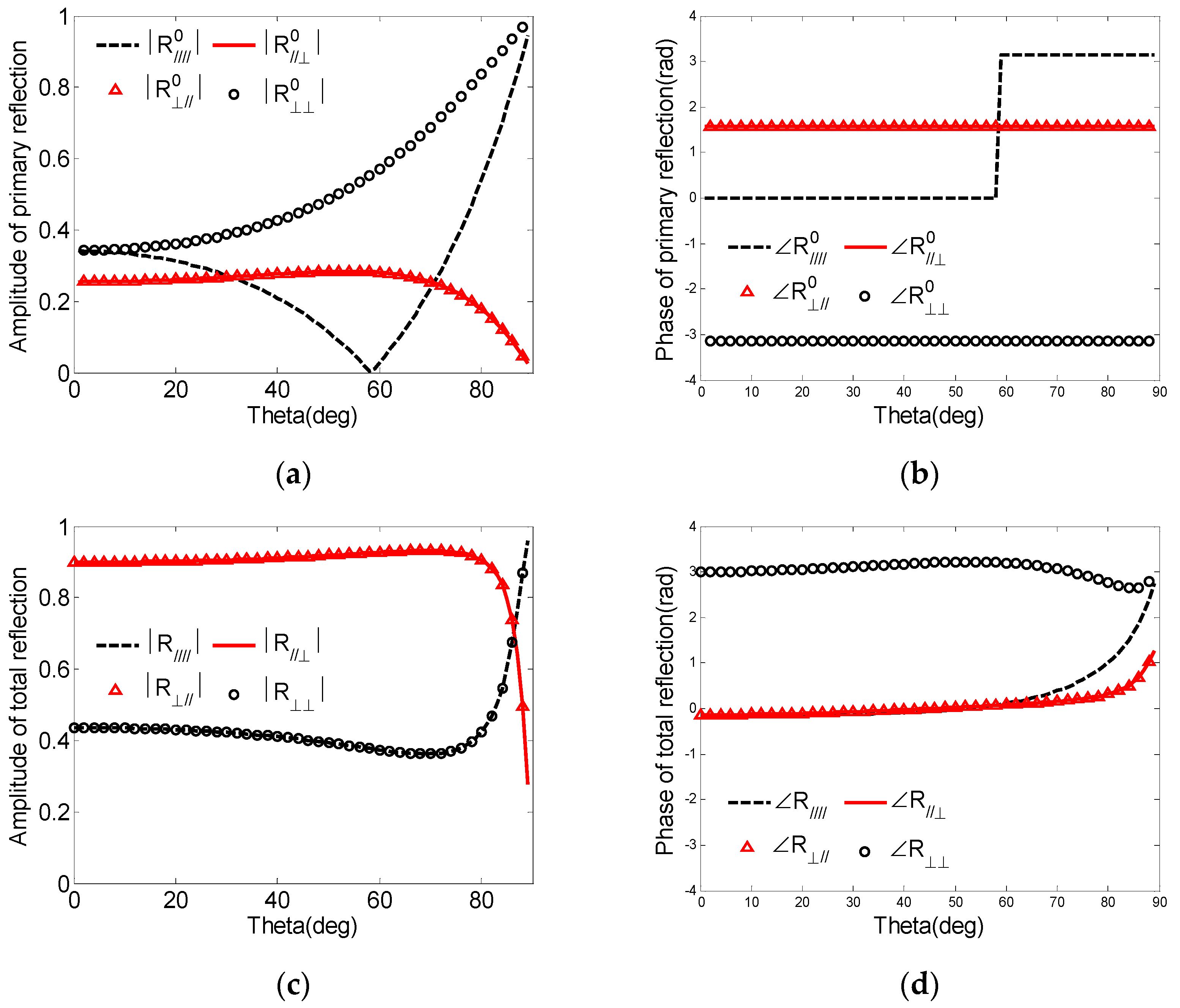
According to the analysis in Section 2, the total spectral scattered field can be decomposed into the primary reflection field on the upper surface and the secondary scattering fields transmitted from the plasma layer. In this section, the numerical curves of the primary reflection on the upper surface and the initial transmission after one reflection in the layer are given, and their relationship with the total scattering is compared and analyzed to explore the contribution of different modes of EM waves to the scattering.
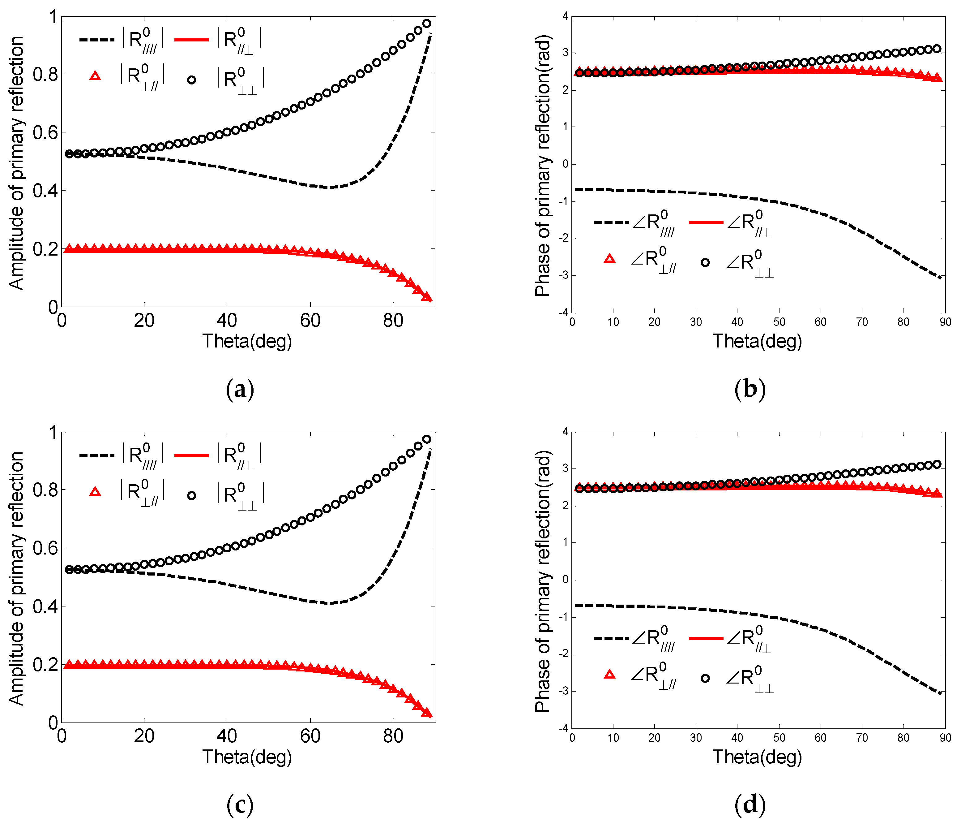
Firstly, the reflection coefficients when the incident angle changes are investigated. Figure 11 and Figure 12, respectively, show the reflection coefficient of lossless and lossy plasma coating varying with the incident angle. The relative permittivity tensor elements of the lossless and lossy plasma, respectively, are and ; the incident angle is ; and the coating thickness is . It can be seen from Figure 11 that when the lossless plasma is coated, the two main polarization components of the primary reflection are not equal, while the two main polarization components of the total reflection are equal. In Figure 12, when the coating plasma is lossy, the two main polarization components of are not equal, and the two main polarization components of are also not equal. Comparing Figure 11 and Figure 12, it can also be found that lossless coating produces stronger cross-polarization than that caused by lossy coating.
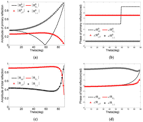
Figure 11.
Amplitude and phase of mode fields in lossless plasma coating: (a) ; (b) ; (c) ; (d) .
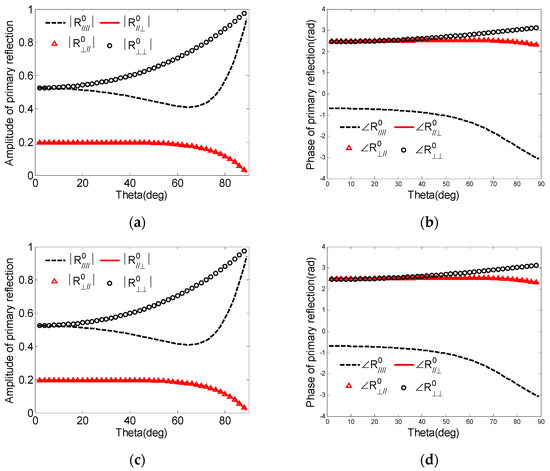
Figure 12.
Amplitude and phase of mode fields in lossy plasma coating: (a) ; (b) ; (c) ; (d) .
Then, the reflection and transmission of mode fields when the coating thickness changes are investigated. The relative permittivity tensor elements of the lossless and lossy plasma, respectively, are and , and the incident angle is .
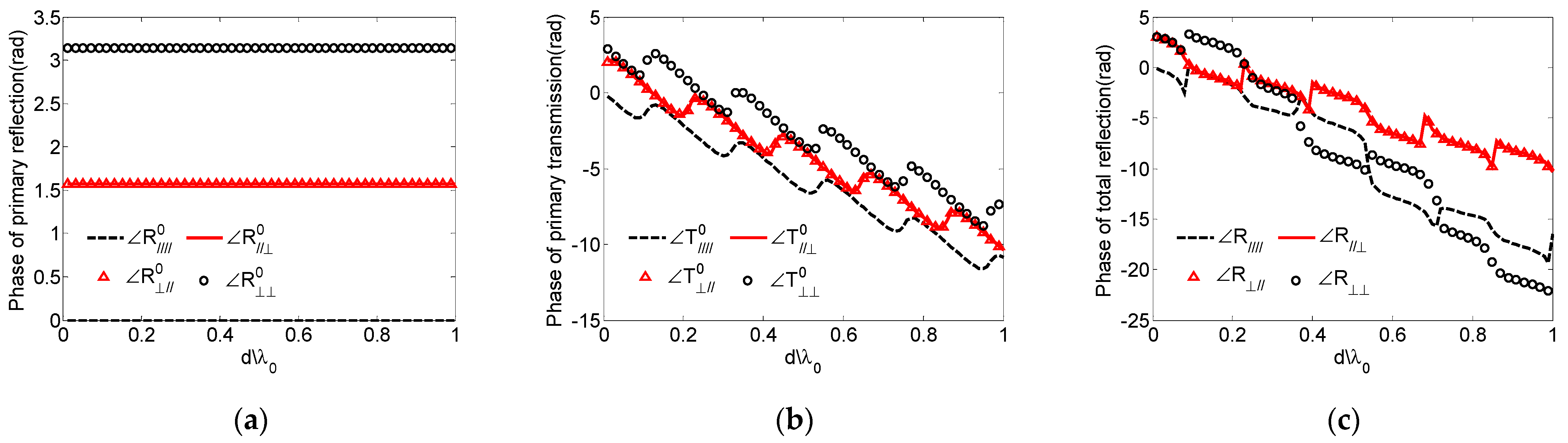
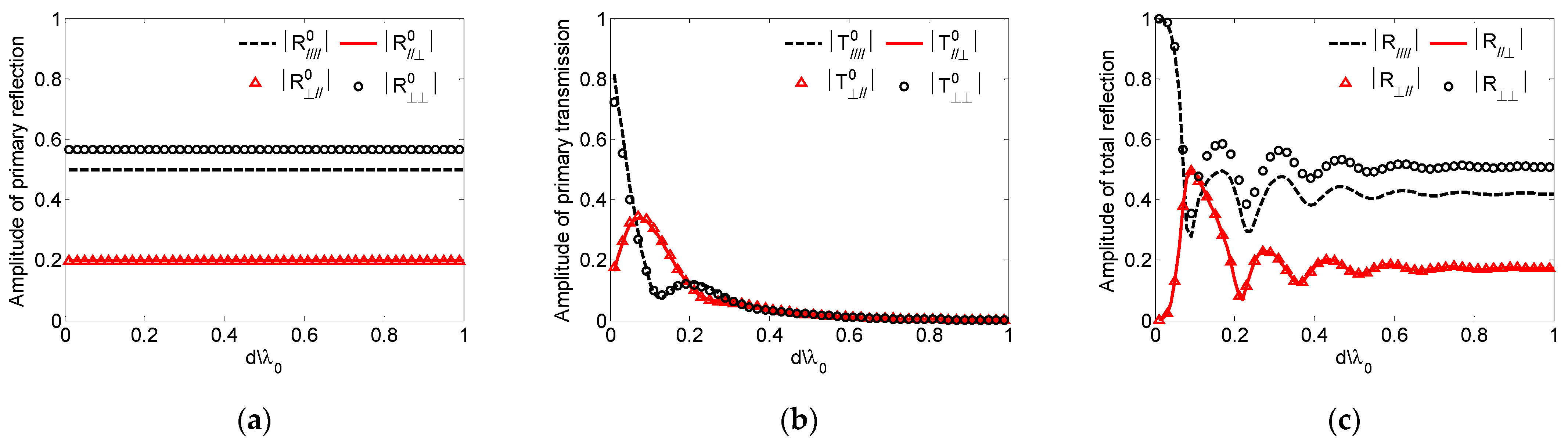
Figure 13 and Figure 14, respectively, show the amplitude and phase of different mode fields varying with coating thickness in the case of lossless plasma coating. It can be seen that each component of the primary reflection is independent of the coating thickness. The amplitude of each component of the initial transmission after one reflection in the layer changes periodically with the coating thickness, and the phase lags continuously with the increase in the thickness. The amplitude of final total reflection also tends to “Periodicity” with the coating thickness, and the phase lags further with the multiple reflections of waves in the layer.
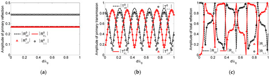
Figure 13.
The amplitude of mode fields in lossless plasma coating: (a) ; (b) ; (c) .
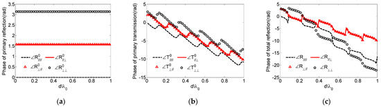
Figure 14.
The phase of mode fields in lossless plasma coating: (a) ; (b) ; (c) .
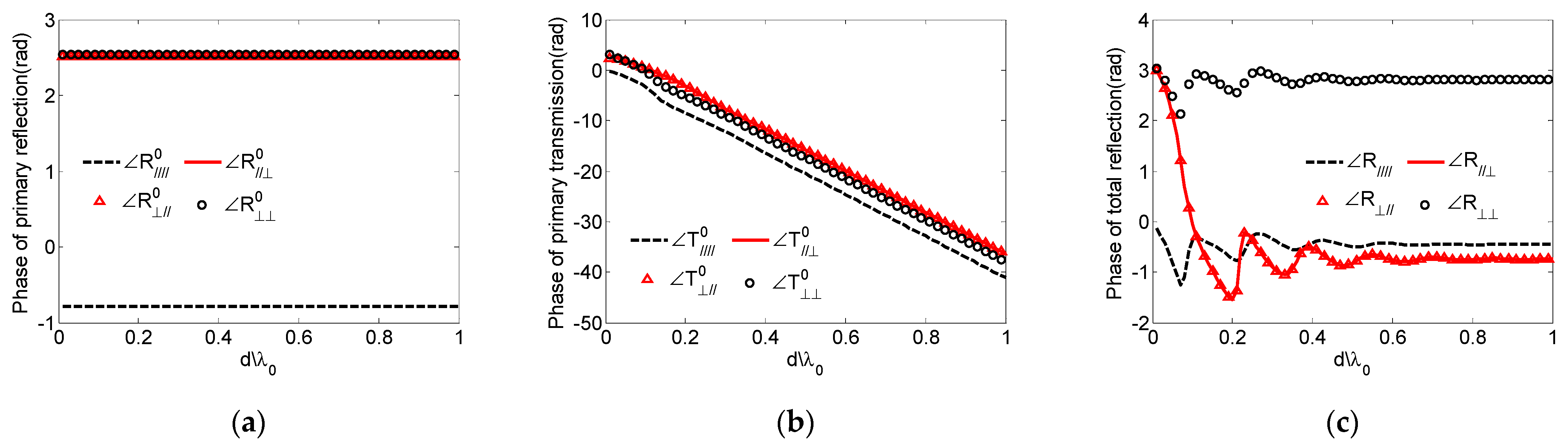
Figure 15 and Figure 16, respectively, show the amplitude and phase of different mode fields varying with coating thickness in the case of lossy plasma coating. At this time, the components of the primary reflection are also independent of the thickness of the coating layer. The amplitude of each component of the initial transmission after one reflection in the layer is already very small, and the amplitude of final total reflection tends to converge with the increase in thickness. This is because when the thickness of the coated lossy plasma layer increases to a certain value, the PEC substrate does not reflect the waves in the anisotropic layer, which is a half-space problem. At this time, the EM wave is completely absorbed in the plasma layer, and the total field will mainly come from the contribution of the primary reflection on the upper surface.

Figure 15.
The amplitude of mode fields in lossy plasma coating: (a) ; (b) ; (c) .
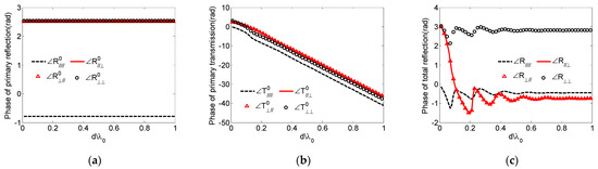
Figure 16.
The phase of mode fields in lossy plasma coating: (a) ; (b) ; (c) .
From Figure 13, Figure 14, Figure 15 and Figure 16, it can be seen that the scattering characteristics of the two coated slabs are completely different. For lossless coating, strong cross-polarization scattering is generated, and the amplitudes of the two main polarization components are equal. However, in the case of lossy plasma coating, the two main polarization components are quite different, and the layer has a strong wave-absorbing ability.
4.3. Scattering Characteristics and Analysis of Plasma-Coated Complex Targets
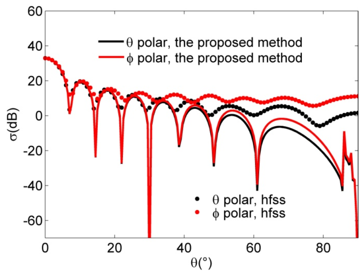
Because it is difficult to find the reference results of scattering from electrically large and complex targets coated with anisotropic plasma in the existing literature, and the commercial software HFSS can calculate the scattering of coated plates, the RCS of anisotropic plasma-coated plates has been calculated by this method and compared with the numerical algorithm of HFSS. Figure 17 shows the monostatic RCS of the rectangular coated plate obtained through this method and HFSS. It can be seen from the figure that the results obtained by the two methods are in good agreement in the range close to normal incidence. When the deviation from normal incidence is large, there is a certain gap between the results obtained by this method and the numerical algorithm. This is because the calculation error of the physical optics algorithm will increase when it deviates greatly from the specular reflection direction. Table 1 lists the time consumed and memory required for the two methods. Obviously, compared with the numerical algorithm, the proposed method requires very little time and memory and is more suitable for the scattering calculation of electrically large and complex targets.

Figure 17.
A plate coated with a plasma layer and its monostatic RCSs against angle . The layer’s thickness is . The incident angle is . The relative permittivity tensor elements are .

Table 1.
The CPU time and required memory of Figure 17.
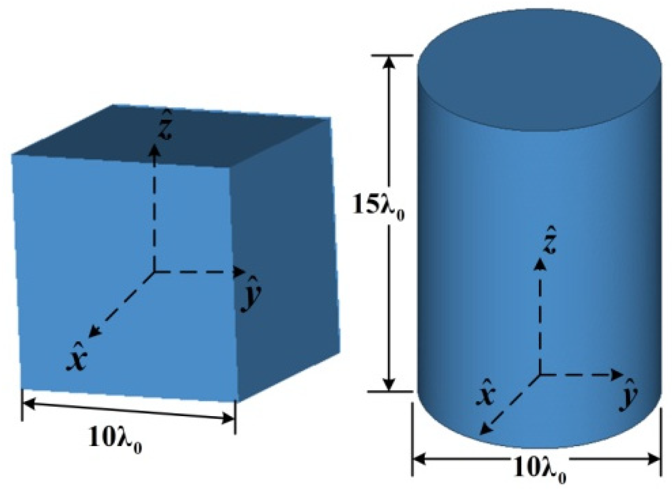
The following will use the spectral domain combined with the physical optics algorithm proposed in this paper to investigate the scattering characteristics of plasma-coated typical bodies and complex targets. These targets include a cube, cylinder, missile, and airplane. In our calculation, the coating thickness is .
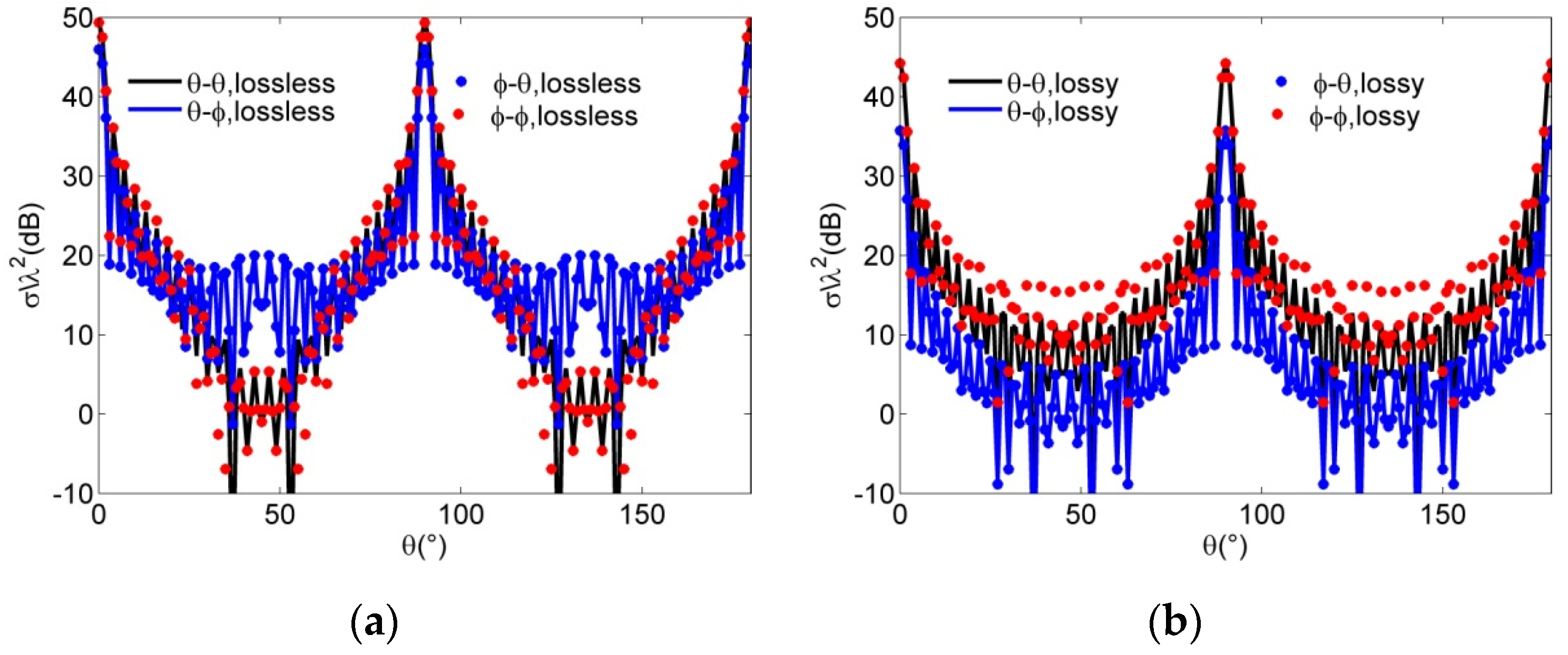
The first object is a plasma-coated cube as shown in Figure 18. Figure 19 presents the monostatic RCSs of the cube coated with lossless and lossy plasma. It can be seen that the lossless plasma coating produces strong cross-polarization scattering, which is much larger than co-polarization scattering. When the lossy plasma coating is used, the cross-polarization scattering is weakened and the co-polarization scattering is enhanced. This means that the anisotropic plasma with off-diagonal dielectric parameters changes the spatial field distribution. This feature can also be seen in the scattering results of other dielectric parameters and other targets in our article.
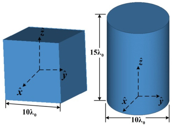
Figure 18.
Models of plasma-coated cube and cylinder.

Figure 19.
Monostatic RCSs from a PEC cube coated with (a) lossless and (b) lossy plasma layer. The relative permittivity tensor elements of the lossless and lossy plasma, respectively, are and ; the incident angle is .
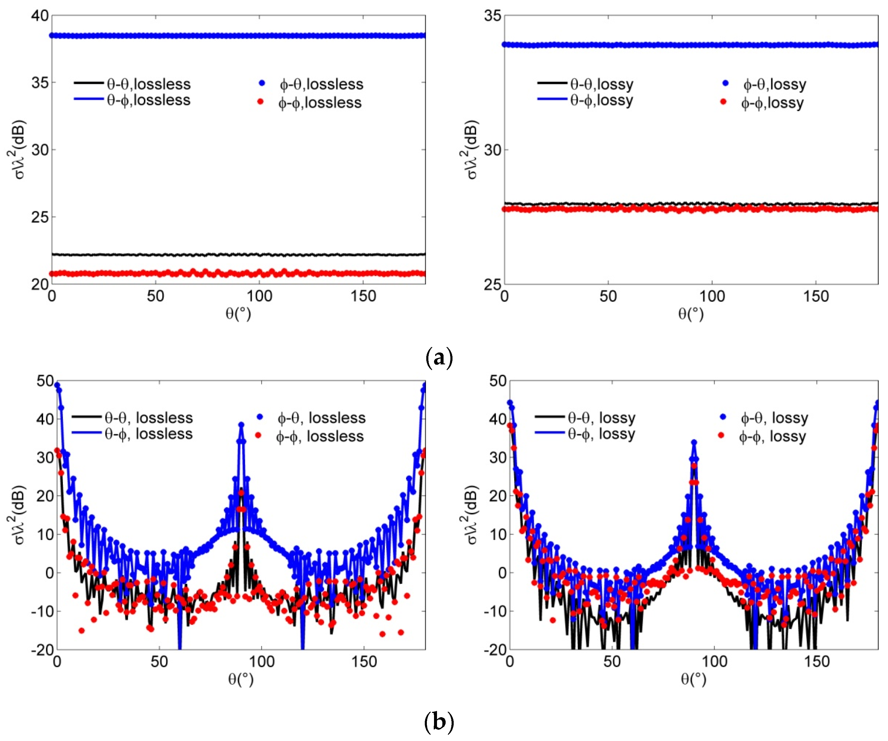
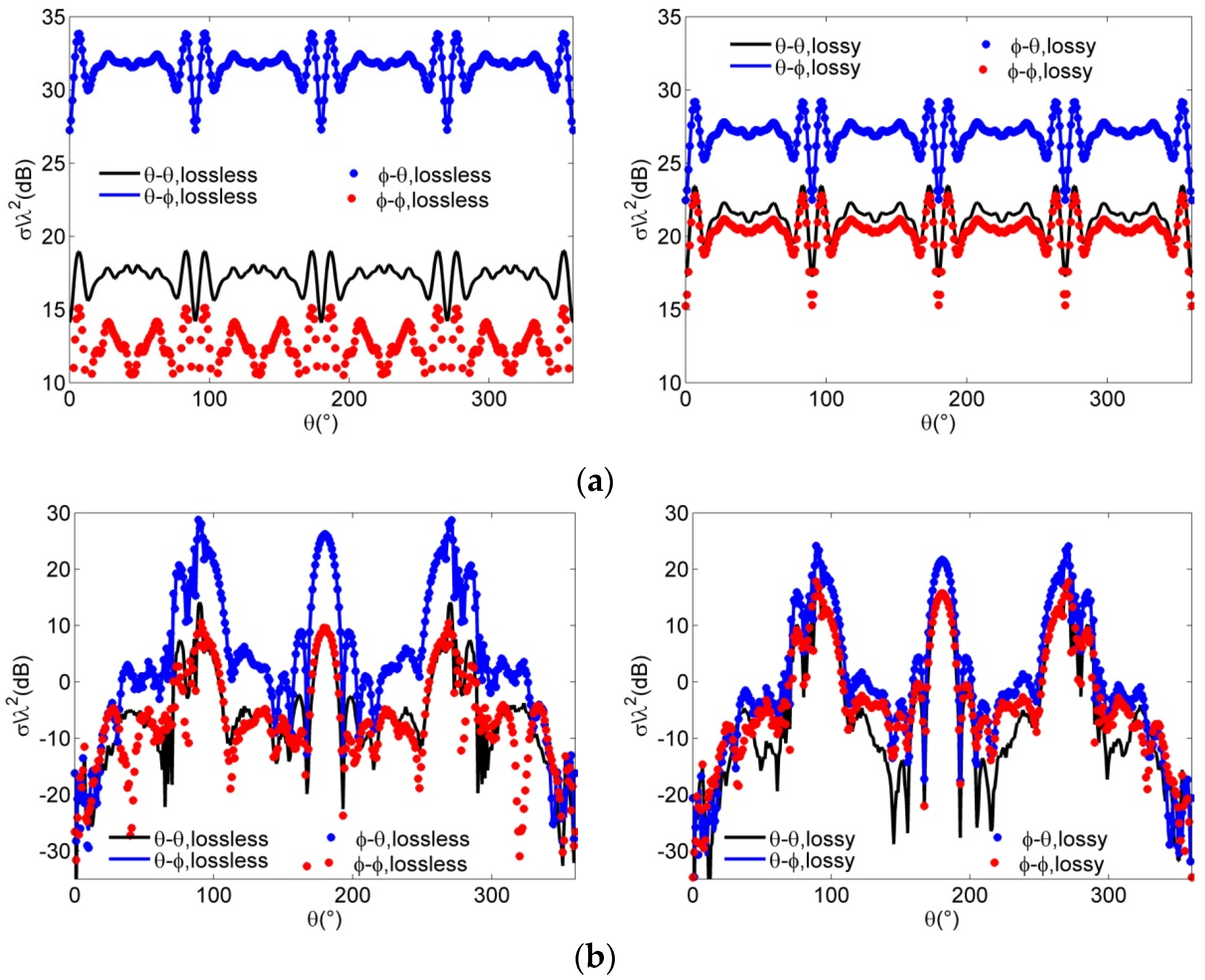
The second target is a coated cylinder as shown in Figure 18. Figure 20 presents the monostatic RCSs of the coated cylinder in the and observation planes. It is observed that strong cross-polarization scattering occurs in both lossy and lossless plasma coating cases. In the roll-plane , the co-polarization RCSs by lossless plasma coating are different but almost equal by lossy plasma coating. In the meridian plane of the cylinder, the situation is the opposite: the co-polarization RCSs by lossless plasma coating are very close but obviously different by lossy plasma coating.

Figure 20.
Monostatic RCSs from a PEC cylinder coated with a plasma layer in (a) and (b) planes. The relative permittivity tensor elements of the lossless and lossy plasma, respectively, are and .
The third example is the coated missile, whose model and observation planes are shown in Figure 21. Figure 22 presents the monostatic RCSs of the coated missile in the and observation planes. Again, strong cross-polarization scattering occurs in both coating cases. The missile’s body is a body of revolution with axis like a cylinder, so it has similar scattering characteristics. In the roll-plane , the co-polarization RCSs by lossless plasma coating are quite different, but very close by lossy plasma coating. In the meridian plane , the situation is the opposite: the co-polarization RCSs by lossless plasma coating are very close but different from lossy plasma coating.
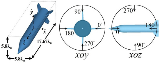
Figure 21.
The geometry of a plasma-coated missile and its observation planes.

Figure 22.
Monostatic RCSs of the plasma-coated missile in (a) and (b) planes. The relative permittivity tensor elements of the lossless and lossy plasma, respectively, are and .
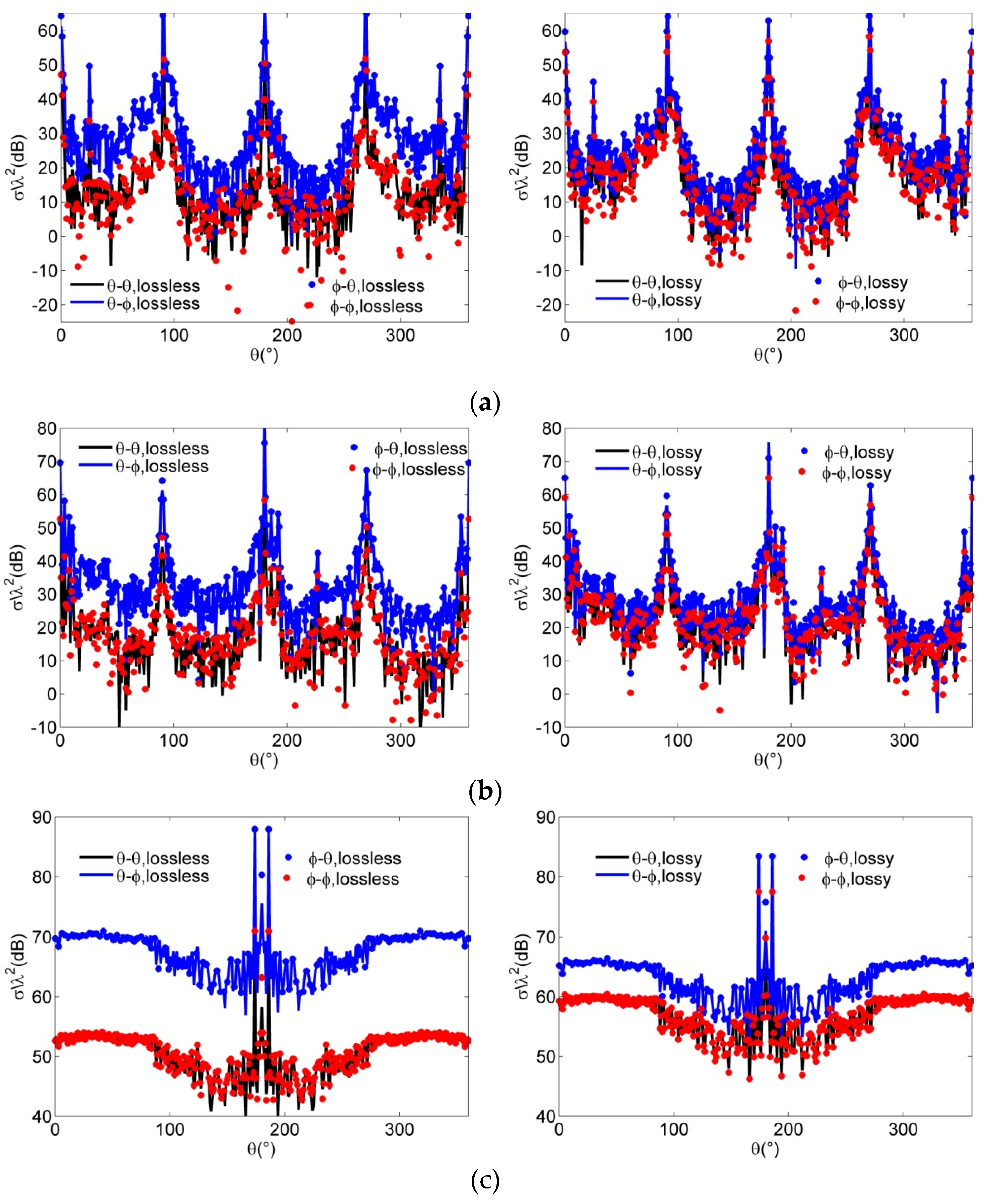
The last example is the coated aircraft shown in Figure 23. Figure 24 shows the monostatic RCSs of the coated aircraft in the three observation planes. Again, compared with the lossless plasma coating, the cross-polarization RCSs decrease while the co-polarization RCSs increase by the lossy plasma coating, and this is especially obvious on the roll-plane . Moreover, for both lossless and lossy plasma coatings, the co-polarization RCSs are relatively close. This shows that the scattering mechanism of the coated aircraft is more complicated than the previous simple bodies.
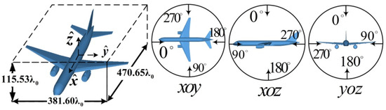
Figure 23.
The geometry of a plasma-coated aircraft and three observation planes.
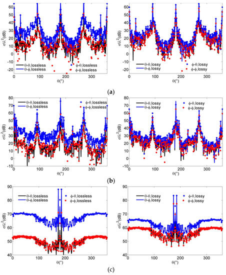
Figure 24.
Monostatic RCSs of the plasma-coated aircraft in three observation planes: (a) , (b) , and (c) . The relative permittivity tensor elements of the lossless and lossy plasma, respectively, are and .
5. Conclusions
A high-frequency algorithm for EM scattering from electrically large and complex targets coated with anisotropic plasma was proposed based on the spectral domain method. Compared with numerical algorithms, the proposed method is effective and has higher computational efficiency. Finally, the high-frequency scattering of plasma-coated electrically large complex targets was estimated and analyzed for the first time, and the RCS of plasma-coated canonical targets and complex targets were given. The numerical results show the inherent cross-polarization scattering phenomenon of magnetized plasma. Its complex interaction with EM waves significantly changes the scattering characteristics of coated targets. Note that the plasma coating studied in this paper is homogeneous, and the method extended to non-uniform plasma coating will be more applicable. Besides, in target stealth design, coating materials at a specific location is usually easier to achieve, and this demand is easy to meet through a little improvement in this method. The scattering characteristics of targets under different plasma parameters can be further explored by this method, so as to provide guidance for engineering applications. In summary, the research results of this paper have important theoretical research value and the engineering application potential in the areas of radar detection and recognition and target stealth design.
Author Contributions
Conceptualization, G.Z.; methodology, Z.R.; formal analysis, G.Z. and Z.R.; investigation, Z.R.; validation, Z.R. and C.L.; writing—original draft preparation, Z.R.; writing—review and editing, S.H. and C.L.; supervision, Z.Y. and J.L. All authors have read and agreed to the published version of the manuscript.
Funding
This research received no external funding.
Acknowledgments
We gratefully thank the anonymous reviewers for their critical comments and constructive suggestions on the manuscript.
Conflicts of Interest
The authors declare no conflict of interest.
References
- Hartunian, R.A.; Stewart, G.E.; Fergason, S.D.; Curtiss, T.J.; Seibold, R.W. Causes and Mitigation of Radio Frequency (RF) Blackout During Reentry of Reusable Launch Vehicles; Aerospace Corporation: El Segundo, CA, USA, 2007. [Google Scholar]
- Kushwaha, M.; Halevi, P. Magnetoplasma modes in thin films in the Faraday configuration. Phys. Rev. B Condens. Matter 1987, 35, 3879–3889. [Google Scholar] [CrossRef] [PubMed]
- Kushwaha, M.; Halevi, P. Magnetoplasmons in thin films in the Voigt configuration. Phys. Rev. B Condens. Matter 1987, 36, 5960–5967. [Google Scholar] [CrossRef]
- Kushwaha, M.; Halevi, P. Magnetoplasmons in thin films in the perpendicular configuration. Phys. Rev. B Condens. Matter 1989, 38, 12428–12435. [Google Scholar] [CrossRef] [PubMed]
- Shi, J.; Gao, Y.; Wang, J.; Yuan, Z.; Ling, Y. Electromagnetic Reflection of Conductive Plane Covered with Magnetized Inhomogeneous Plasma. Int. J. Infrared Millim. Waves 2001, 22, 1167–1175. [Google Scholar] [CrossRef]
- Zhang, J.; Liu, Z. Electromagnetic Reflection from Conductive Plate Coated with Nonuniform Plasma. Int. J. Infrared Millim. Waves 2007, 28, 71–78. [Google Scholar] [CrossRef]
- Schneider, J.; Hudson, S. A finite-difference time-domain method applied to anisotropic material. IEEE Trans. Antennas Propag. 1993, 41, 994–999. [Google Scholar] [CrossRef]
- Heald, M.A.; Wharton, C.B.; Furth, H.P. Plasma diagnostics with microwaves. Phys. Today 1965, 18, 72–74. [Google Scholar] [CrossRef]
- Vidmar, R.J. On the use of atmospheric pressure plasmas as electromagnetic reflectors and absorbers. IEEE Trans. Plasma Sci. 1990, 18, 733–741. [Google Scholar] [CrossRef]
- Cheng, G.; Liu, L. Direct finite-difference analysis of the electromagnetic-wave propagation in inhomogeneous plasma. IEEE Trans. Plasma Sci. 2010, 38, 3109–3115. [Google Scholar] [CrossRef]
- Geng, Y.; Qiu, C. Extended Mie Theory for a Gyrotropic-Coated Conducting Sphere: An Analytical Approach. IEEE Trans. Antennas Propag. 2011, 59, 4364–4368. [Google Scholar] [CrossRef]
- Song, Y.; Tse, C.; Qiu, C. Electromagnetic Scattering by a Gyrotropic-Coated Conducting Sphere Illuminated From Arbitrary Spatial Angles. IEEE Trans. Antennas Propag. 2013, 61, 3381–3386. [Google Scholar] [CrossRef]
- Ghaffar, A.; Yaqoob, M.Z.; Alkanhal, M.; Sharif, M.; Naqvi, Q. Electromagnetic scattering from anisotropic plasma-coated perfect electromagnetic conductor cylinders. AEU-Int. J. Electron. Commun. 2014, 68, 767–772. [Google Scholar] [CrossRef]
- Soudais, P.; Steve, H.; Dubois, F. Scattering from several test-objects computed by 3-D hybrid IE/PDE methods. IEEE Trans. Antennas Propag. 1999, 47, 646–653. [Google Scholar] [CrossRef]
- Graglia, R.; Uslenghi, P.; Zich, R. Moment Method with Isoporametric Element for Three-Dimensional A nisotropic Scatterers. Proc. IEEE 1989, 77, 750–760. [Google Scholar] [CrossRef]
- Yuan, J.; Niu, Z.; Gu, C. Electromagnetic Scattering by Arbitrarily Shaped PEC Targets Coated with Anisotropic Media Using Equivalent Dipole-Moment Method. J. Infrared Millim. Terahertz Waves 2010, 31, 744–752. [Google Scholar] [CrossRef]
- Chung, S.S.M. FDTD simulations on radar cross sections of metal cone and plasma covered metal cone. Vacuum 2012, 86, 970–984. [Google Scholar] [CrossRef]
- Liu, S.; Zhong, S. Analysis of backscattering RCS of targets coated with parabolic distribution and time-varying plasma media. Optik-Int. J. Light Electron. Opt. 2013, 124, 6850–6852. [Google Scholar] [CrossRef]
- Xu, L.; Yuan, N. FDTD Formulations for Scattering From 3-D Anisotropic Magnetized Plasma Objects. IEEE Antennas Wirel. Propag. Lett. 2006, 5, 335–338. [Google Scholar] [CrossRef]
- Sheng, X.; Peng, Z. Analysis of scattering by large objects with off-diagonally anisotropic material using finite element-boundary integral-multilevel fast multipole algorithm. IET Microw. Antennas Propag. 2010, 4, 492–500. [Google Scholar] [CrossRef]
- Wanjun, S.; Hou, Z. RCS Prediction of Objects Coated by Magnetized Plasma Via Scale Model With FDTD. IEEE Trans. Microw. Theory Tech. 2017, 65, 1939–1945. [Google Scholar] [CrossRef]
- Dan, L.; Tong, C.; Jiao, W. RCS simulation of plasma-coated targets modeled by NURBS surfaces. In Proceedings of the 2009 Asia Pacific Microwave Conference, Singapore, 7–10 December 2009. [Google Scholar]
- Liu, S.; Guo, L. Analyzing the Electromagnetic Scattering Characteristics for 3-D Inhomogeneous Plasma Sheath Based on PO Method. IEEE Trans. Plasma Sci. 2016, 44, 2838–2843. [Google Scholar] [CrossRef]
- Yu, Q.; Cong, Z.; He, Z.; Ding, D.; Chen, R. Study on Electromagnetic Scattering Characteristic of Hypervelocity Model with SBR Method. In Proceedings of the 2018 IEEE International Conference on Computational Electromagnetics (ICCEM), Chengdu, China, 26–28 March 2018. [Google Scholar]
- Bian, Z.; Li, J.; Guo, L.; Luo, X. Analyzing the Electromagnetic Scattering Characteristics of a Hypersonic Vehicle Based on the Inhomogeneity Zonal Medium Model. IEEE Trans. Antennas Propag. 2021, 69, 971–982. [Google Scholar] [CrossRef]
- Li, J.; Bao, H.; Ding, D. Analysis for Scattering of Non-homogeneous Medium by Time Domain Volume Shooting and Bouncing Rays. Appl. Comput. Electromagn. Soc. J. 2021, 36, 245–251. [Google Scholar] [CrossRef]
- Yang, B.; Chen, R.; He, Z.; Yin, H. A Tetrahedral Meshed SBR method for RCS of plasma-coated cavity. In Proceedings of the 2019 International Applied Computational Electromagnetics Society Symposium-China (ACES), Nanjing, China, 8–11 August 2019; pp. 1–3. [Google Scholar] [CrossRef]
- Platzman, P.M.; Ozaki, H.T. Scattering of Electromagnetic Waves from an Infinitely Long Magnetized Cylindrical Plasma. J. Appl. Phys. 1960, 31, 1597–1601. [Google Scholar] [CrossRef]
- Yeh, K.C.; Liu, C.H. Theory of ionospheric waves. IEEE Trans. Plasma Sci. 1972, 1, 42. [Google Scholar] [CrossRef]
- Yao, J.; He, S.; Li, C.; Yin, H.; Wang, C.; Zhu, G. An asymptotic solution of the scattering from a biaxial electric anisotropic slab with a PEC substrate. J. Electromagn. Waves Appl. 2013, 27, 1534–1549. [Google Scholar] [CrossRef]
- Yao, J.J.; He, S.Y.; Zhang, Y.H.; Yin, H.C.; Wang, C.; Zhu, G.Q. Evaluation of Scattering from Electrically Large and Complex PEC Target Coated with Uniaxial Electric Anisotropic Medium Layer Based on Asymptotic Solution in Spectral Domain. IEEE Trans. Antennas Propag. 2014, 62, 2175–2186. [Google Scholar] [CrossRef]
- Wait, J.R. Some boundary value problems involving plasma media. J. Res. Natl. Bur. Stand. 1961, 65, 137–150. [Google Scholar] [CrossRef]
- Elking, D.M.; Roedder, J.M.; Car, D.D.; Alspach, S.D. A review of high-frequency radar cross section analysis capabilities at McDonnell Douglas Aerospace. IEEE Antennas Propag. Mag. 1995, 37, 33–42. [Google Scholar] [CrossRef]
- Gordon, W. Far-field approximations to the Kirchoff-Helmholtz representations of scattered fields. IEEE Trans. Antennas Propag. 1975, 23, 590–592. [Google Scholar] [CrossRef]
- Titchener, J.B.; Willis, J.R. The reflection of electromagnetic waves from stratified anisotropic media. IEEE Trans. Antennas Propag. 1991, 39, 35–39. [Google Scholar] [CrossRef]


Publisher’s Note: MDPI stays neutral with regard to jurisdictional claims in published maps and institutional affiliations. |
© 2022 by the authors. Licensee MDPI, Basel, Switzerland. This article is an open access article distributed under the terms and conditions of the Creative Commons Attribution (CC BY) license (https://creativecommons.org/licenses/by/4.0/).