1. Introduction
The exploitation of Global Navigation Satellite System (GNSS) signals scattered off Earth’ surface for remote sensing purposes was first demonstrated in the late 1980s by Hall and Cordy [
1] and, later, by Martin-Neira for ocean altimetry [
2]. Since then, GNSS-Reflectometry (GNSS-R) concepts and systems have been successfully applied in numerous Earth observation applications over ocean [
3,
4], land [
5,
6] and cryosphere [
7,
8]. For a deep review of GNSS-R principles, missions and applications, the interested reader is referred to [
9].
A traditional application of GNSS-R data over oceans is the analysis of the sea state, including the estimation of the wind speed and root mean square (RMS) sea surface slope. To boost sea state retrieval performance, GNSS-R receivers are typically designed to acquire and process the signal coming from a portion of sea surface surrounding the specular reflection point, i.e., the so-called
glistening zone, where most electromagnetic (EM) energy of the sea echo is reflected. Additionally, cross- and de-polarization effects due to sea surface make the right-hand circular polarization (RHCP)-transmitted signal mostly scattered in left-hand circular polarization (LHCP). Accordingly, past and current GNSS-R receivers are typically equipped with an LHCP receiving channel, while the presence of also an RHCP channel is left so far to biomass and soil moisture retrieval using polarimetric GNSS-R measurements [
10]. Here, we refer to such forward-scattering GNSS-R receivers collecting the LHCP component of the scattered signal as
conventional GNSS-R.
Recent applications of conventional GNSS-R, including the ongoing NASA CYGNSS mission, focus on both ocean and land remote sensing, see e.g., [
11,
12,
13,
14]. Additionally, in the last decade, GNSS-R has been investigated for ship detection applications [
15,
16,
17], where it might offer important and intriguing advantages compared to other remote sensing technologies, including synthetic aperture radar (SAR) and optical/multi-spectral sensors. As a matter of fact, GNSS-R allows for global and seamless monitoring of the Earth’ surface using low-cost, light-weight receivers that can count on the free availability of >100 GNSS signal sources, including GPS, GLONASS, Galileo, and BeiDou-2. Revisit time offered by GNSS-R systems can be as low as few hours when launched in constellation formation and can be further improved by tracking multiple GNSSs [
17]. Such key factors make GNSS-R an intriguing, despite not yet mature, technology for near real-time maritime surveillance [
18]. Indeed, feasibility of ship detection using GNSS-R data is still an open issue and requires further investigations.
Ship detection using GNSS-R has been investigated in numerous works, ranging from theoretical [
16,
19,
20], simulation [
21] and experimental [
15,
17,
22] analyses. The general consensus of all such works is that conventional GNSS-R is scarcely suited to the ship detection problem, especially from spaceborne altitudes, due to the extremely poor GNSS power density-that can be as low as
at the Earth’ surface-, and GNSS-R spatial resolution, that can be as large as tens of kilometers over oceans.
Besides this intrinsic limitation of the GNSS power budget, additional issues are related to the acquisition geometry and polarization of conventional GNSS-R. Indeed, in the presence of a ship within the observation area, the different mechanisms arising in the EM interaction between sea surface and ship, namely multiple reflections, make only a negligible quota of the ship echo be scattered in LHCP and in the specular direction [
21,
23], and, then, collected by conventional GNSS-R receivers. Conversely, double-bounce ship-sea and sea-ship scattering contributions, which are predominant in most acquisition configurations, are stronger in far-from-specular directions due to the mirror-like behavior of the ship hull, the direction of the ship peak radiation depending on the orientation of the ship against the transmitter [
23]. Additionally, the metallic ship hull leads to a polarization inversion of the impinging signal, that, after a further reflection upon the sea surface, is mostly in RHCP, as the transmitting one. All such aspects strongly affect target visibility in conventional GNSS-R data and compromise reliable maritime surveillance using GNSS-R systems.
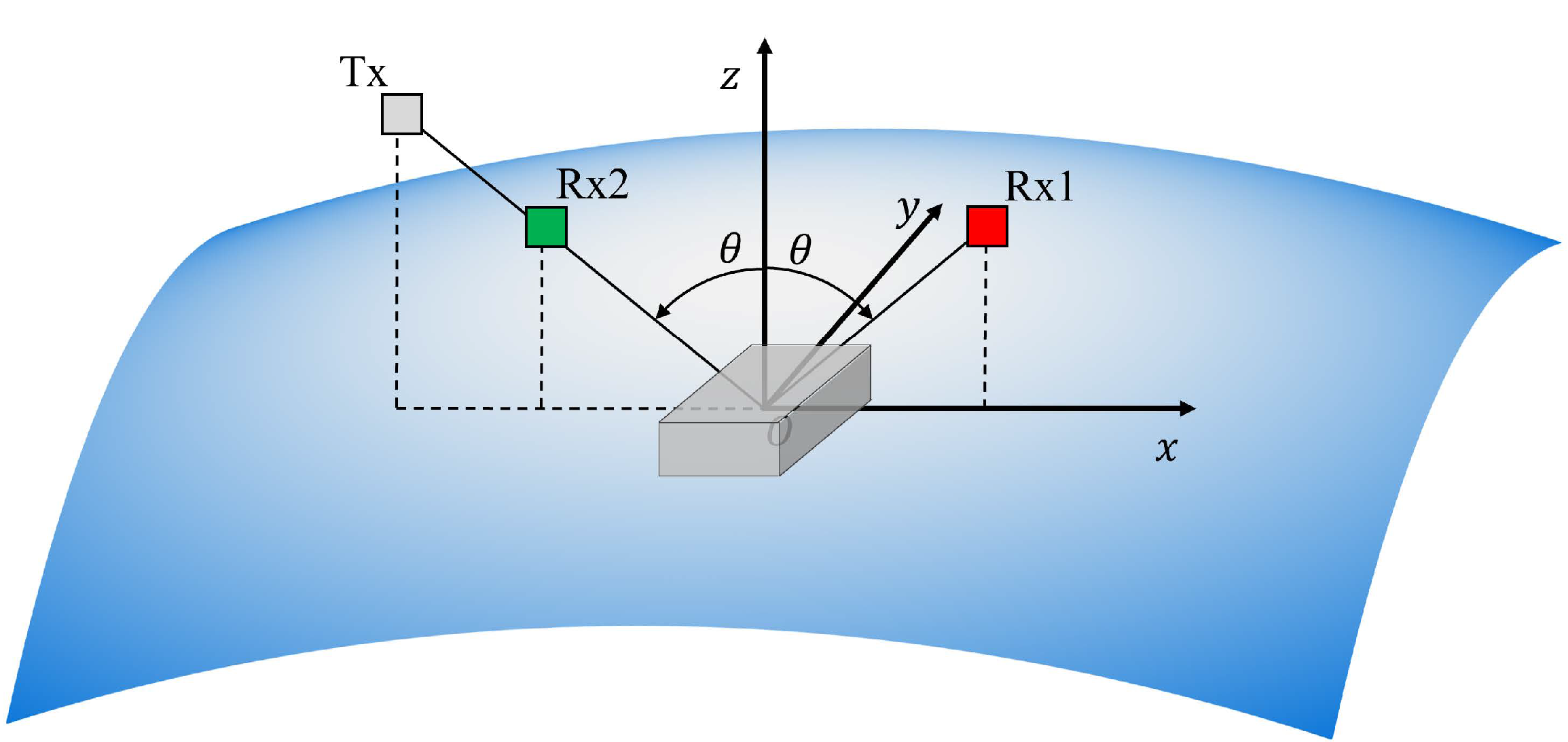
In order to overcome these severe limitations of conventional GNSS-R, ad-hoc GNSS-R instruments specifically designed for ship detection applications were envisaged in [
20]. Such receivers are conceived to work in a backscattering configuration rather than the conventional forward-scattering one and equipped with an RHCP channel instead of the LHCP one. Here, these RHCP back-scattering GNSS-R instruments are referred to as
unconventional GNSS-R. A graphical comparison of conventional and unconventional GNSS-R systems is depicted in
Figure 1.
The benefits of the backscattering geometry were highlighted first in [
16] and then proved theoretically in [
19] by means of a link budget analysis using the analytical model for the ship radar cross section (RCS) presented in [
23], while expected performance of unconventional GNSS-R have been assessed on both a theoretical and a simulation basis in [
20,
21], respectively. In particular, in [
21] it was demonstrated that best detection performance is achieved with intermediate viewing angles, low wind speed, and ship perfectly facing the transmitter, i.e., ship hull normal to the mean incidence plane. In such configurations, signal-to-noise-clutter ratio for the ship target return larger than 7 dB were obtained from airborne altitudes.
However, performance analyses carried out in such previous works are based on the fundamental assumption that sea clutter can be reliably described by means of the Geometrical Optics (GO) model, which represents the sea surface scattering model commonly adopted within the GNSS-R community [
9]. Indeed, it is well known that GO can accurately predict sea surface scattering at microwaves in far-from-grazing incidence and only in a rather narrow angular region including the forward-scattering direction, whereas it significantly underestimates diffuse scattering outside this region [
24,
25]. Additionally, GO cannot catch cross- and de-polarization effects arising in the incidence plane as it is derived under the tangent plane approximation. Accordingly, an accurate investigation, design and simulation of unconventional GNSS-R systems for maritime surveillance applications might call for a more appropriate modeling of sea surface scattering in L-band, where GNSSs operate, and in a wide set of observation directions.
In this paper, we aim at providing useful guidelines for a fast and accurate simulation of the sea-reflected GNSS signal at any imaging geometry, polarization channel, and sea state. Such guidelines could be fruitfully exploited in future research activities for a more accurate analysis of the expected detection performance using GNSS-R in unconventional configurations and could then support the design of ship-detection-oriented GNSS-R systems. To this end, we carry out an analysis of the signal-to-noise ratio (SNR) for the sea-reflected GNSS signal in arbitrary acquisition geometries. This is accomplished by providing an estimate of the strength of the sea-reflected signal, and, then, of the related SNR by accounting for the thermal noise power.
Sea surface scattering is here described via the recent Bistatic Anisotropic Polarimetric Two-Scale Model (BA-PTSM), which provides an accuracy comparable to other advanced scattering models, e.g., the second-order Small Slope Approximation (SSA2), but at a much reduced computational complexity [
26]. Accordingly, BA-PTSM is a good candidate for fast and accurate simulation of Earth-reflected GNSS signals over wide regions. Additionally, we also investigate the limits of applicability of the GO model for the scope of simulation of unconventional GNSS-R systems, which are conceived to work in far-from-specular acquisition geometries, where classical GO is expected to fail. GNSS-R processing chain and receive antenna beamwidth are accounted for as well for the evaluation of the sea-reflected signal SNR. Similar analyses were presented in [
27,
28]. Here we extend such analyses considering a wider set of acquisition geometries, and, additionally, provide a more general expression for the received signal strength which allows for more accurate results as discussed in detail in the following sections.
The main outcomes of our study could support a fast and reliable simulation of sea-reflected GNSS signals in arbitrary imaging geometries, including the backscattering direction. It is worth mentioning that all previous works focusing on unconventional GNSS-R systems do not analyze the effects of the signal processing chain, which, however, is recognized as a key factor influencing ship target detectability as well. This research line is left to future investigations.
The remainder of this paper is organized as follows:
Section 2 briefly describes the BA-PTSM which is used in this work for modeling sea surface scattering in both near- and far-from-specular observation directions;
Section 3 presents the power budget analysis for the sea-reflected GNSS signal;
Section 4 describes and discusses numerical results of the SNR analysis for spaceborne and airborne GNSS-R. Finally, main conclusions are drawn in
Section 5.
2. Bistatic Anisotropic Polarimetric Two-Scale Model
Sea surface scattering is here described via the BA-PTSM, a recent advanced scattering model suited to anisotropic surfaces and bistatic geometries [
26]. It is an evolution of the original two-scale model (TSM) firstly proposed about fifty years ago to evaluate EM scattering from random rough surfaces [
29], including sea surfaces [
30]. Within TSM, the scattering surface is expressed as the superposition of two random rough surfaces at different scales: a small-scale roughness whose horizontal scale is comparable to the EM wavelength and whose height is much smaller than wavelength; a large-scale roughness, whose horizontal scale is very large with respect to wavelength and height comparable to wavelength or larger. Scattering from the small-scale roughness is responsible for diffuse scattering, i.e., scattering in far-from-specular observation directions, and is modeled according to the Small Perturbation Method (SPM) [
31]. Conversely, scattering from large-scale roughness accounts for scattering at and around the specular reflection direction and is described through GO. Accordingly, within TSM, surface scattering is completely characterized by the power spectral density (PSD) of the small-scale roughness (also referred to as surface spectrum) and by the probability density function (PDF) of the large-scale roughness slopes.
The TSM described in [
29,
30] allows for closed-form expressions of only the co-polarized normalized RCS (NRCS), which are obtained by a proper combination of the large- and small-scale scattering contributions. As a matter of fact, a fully polarimetric analysis of the scattered field requires an appropriate modeling of cross- and de-polarization effects, even within the incidence plane. This in turn calls for an accurate evaluation of the off-diagonal terms of the covariance matrix. However, such covariance matrix entries can be obtained only by averaging the SPM term over the large-scale roughness PDF. In the original formulation of TSM, this is accomplished via numerical evaluation of four-fold integrals, which is computationally demanding. Accordingly, TSM cannot be fruitfully exploited in applications where real-time monitoring of wide regions is crucial. In order to overcome this limitation, a fully polarimetric closed-form evaluation of the scattered field can be obtained using Polarimetric TSM (PTSM), which is based on a second-order power series expansion of the tilted-facet SPM covariance matrix around zero large-scale slopes [
32]. Accordingly, PTSM is applicable to large-scale RMS slopes up to 0.3 [
32].
PTSM was originally derived for monostatic radar systems, e.g., SAR, and, therefore, it is suited to an accurate evaluation of the backscattered signal strength. Later, PTSM has been extended to anisotropic surfaces in the so-called Anisotropic PTSM (A-PTSM) in [
33] and, further, to the bistatic case (BA-PTSM) in [
26].
In order to implement BA-PTSM, the PSD of the small-scale roughness and the PDF of the slopes of the large-scale roughness must be specified. The two-dimensional (2-D) anisotropic surface spectrum is expressed around the Bragg resonant surface wavenumber as [
26]
where
and
stand for the module and phase of the surface wavenumber vector;
is the omnidirectional part of the 2-D surface spectrum and
is the angular spreading function, which accounts for the anisotropy of the scattering surface. In BA-PTSM, the small-scale roughness PSD
is described via the high-frequency portion of the Elfouhaily spectrum, whose detailed expression is reported in [
33]. However, around the Bragg resonant wavenumber, it can be approximated as in (
1) with
where for sea surfaces
and
,
and
are parameters depending on wind speed and direction [
33]. More specifically,
is the amplitude coefficient of the omnidirectional part of the power-law PSD of small-scale roughness;
regulates the amplitude oscillations of the angular spreading function;
is directly related to wind direction. The actual expression and definition of such parameters are of no concern here and, therefore, are omitted for the sake of brevity. However, they can be found in [
33].
Large-scale roughness slopes are modeled as jointly Gaussian zero-mean random variables, whose variances and correlation coefficient, again, depend on wind speed and direction as detailed in [
26]. More specifically, such wind-driven variances are modeled according to the Katzberg model in [
34] properly extended to a wider frequency range.
According to polarimetric scattering theory (see e.g., [
35]), under BA-PTSM, the scattered field is described by means of the polarimetric covariance matrix. Each matrix entry
is then expressed as the sum of the large-scale roughness scattering contribution evaluated via GO
, and the small-scale roughness scattering contribution
, evaluated as the SPM term relevant to the generic tilted facet averaged over the large-scale slopes. The SPM term for the generic facet is calculated assuming the small-scale roughness PSD defined in (
1)–(
3). Accordingly,
where the subscripts
p,
q,
r and
s may each stand for horizontal and vertical polarization, and
denotes the ensemble average over the large-scale slopes
and
. The rationale for deriving
and
and their detailed expressions are reported in [
26] and are here omitted for the sake of brevity.
Finally, it is worth mentioning that an intrinsic feature of TSM and its generalizations, including BA-PTSM, is the cutoff wavenumber, i.e., the surface wavenumber separating the small-scale roughness from the large-scale one. The choice of the cutoff wavenumber has a certain degree of arbitrariness and might heavily influence the scattering evaluation. Therefore, it is commonly regarded as an intrinsic limitation of TSMs. Nevertheless, it has been demonstrated that BA-PTSM is only slightly affected by the choice of the cutoff wavenumber, whose effects on scattering predictions are non-negligible only for scattering directions in the very narrow angular region where GO and SPM results are comparable [
26].
3. Link Budget for the GNSS-R Sea Surface Return
The evaluation of the strength of the GNSS signal reflected from the sea surface is carried out by assuming the standard two-step GNSS-R processing chain:
Coherent integration: The signal received through the reflection path is correlated with a properly delayed and frequency-shifted version of either the direct signal or a locally-generated clean replica of the transmitted GNSS signal. The output of this step is a 2-D map of the signal power distribution in the delay-Doppler domain. It is commonly referred to as single-snapshot delay-Doppler map (DDM).
Incoherent integration: The coherently-integrated DDM suffers from a very low SNR due to the poor GNSS Effective Isotropical Radiated Power (EIRP), especially at spaceborne altitudes. Accordingly, a strong noise reduction is necessary for enabling meaningful geophysical information retrieval. This is accomplished by incoherently averaging subsequent single-snapshot DDMs, i.e., by temporal multilook, which reduces the thermal noise power by the factor , where is the number of averaged DDMs.
Typical coherent
and incoherent
integration times are reported in
Table 1 for both spaceborne and airborne receivers.
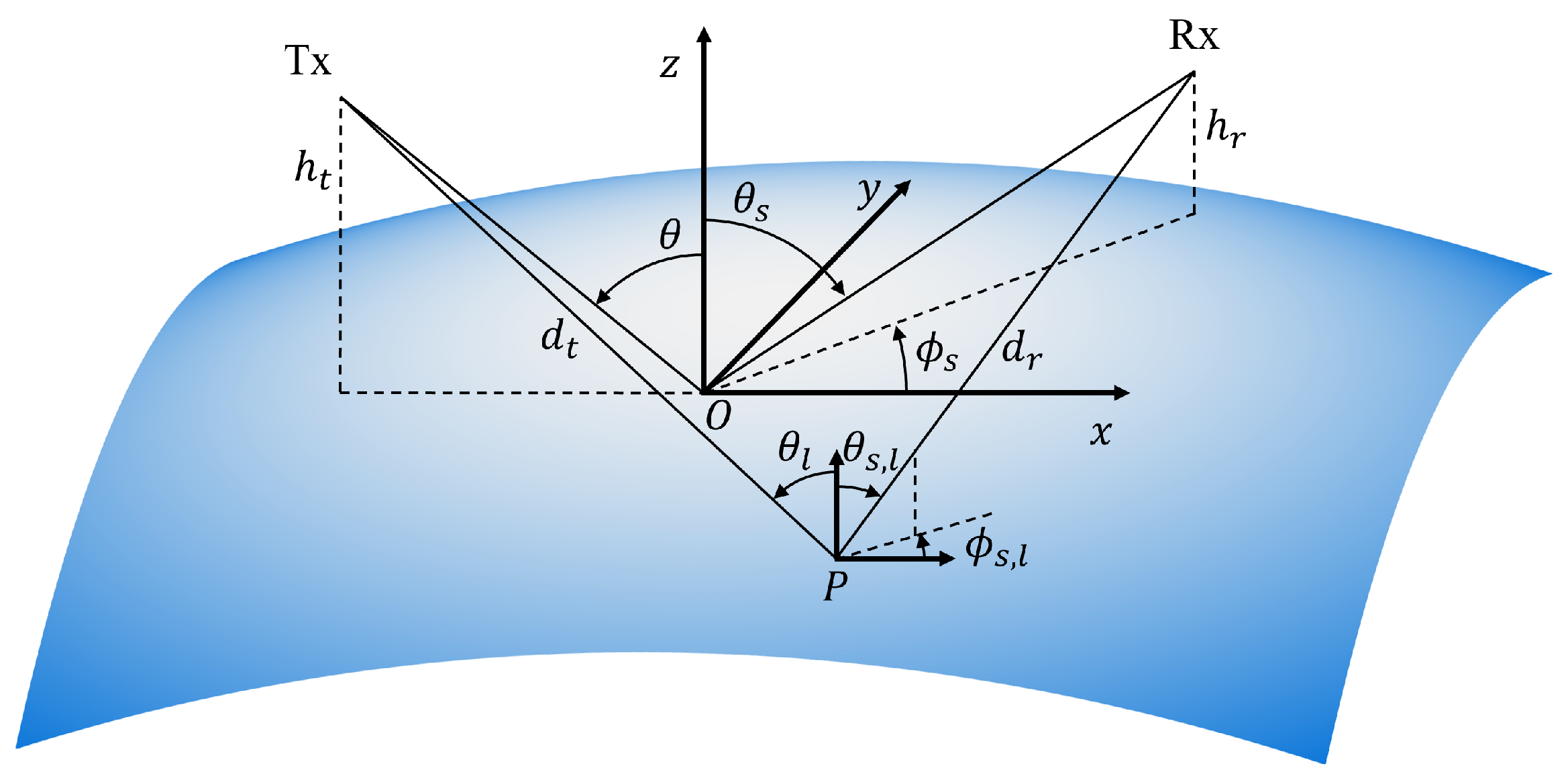
The reference system is shown in
Figure 2: it is defined such that the incident wavevector is in the
x-
z plane and the
z-axis is normal to the mean sea surface plane. Consequently, the transmitter position is fully defined by the viewing angle
, whereas the GNSS-R receiver by the zenith
and azimuth
scattering angles. It is worth noting that in this reference system, the backscattering direction is defined by
and
, while the forward-scattering configuration, typical of conventional GNSS-R, by
and
.
Let’s consider the power of the sea surface echo coming from the resolution cell whose central point is the origin of the reference system in
Figure 2. It turns out that the scattering reference frame depicted in
Figure 2 coincides with the plane tangent to the spherical Earth’ surface in the center of the resolution cell under analysis.
At the output of the incoherent integration, this received power can be written as
where
stands for the
local GNSS transmitter viewing angle,
and
are the
local zenith and azimuth scattering angles, respectively, see
Figure 2. For their evaluation, here we assume a spherical Earth model with radius
km, so that the generic surface point is
with
. Actually, for the scope of evaluating local viewing and scattering angles, sea surface roughness is neglected. Remaining symbols are defined in
Table 1. In (
5),
and
are the transmitter-surface point and receiver-surface point distances, respectively. Moreover, the integration domain is practically limited by the intersection of the transmit and receive antenna patterns and the delay-Doppler resolution cell. The width of the resolution cell in the delay-Doppler domain is
, where
and
are approximately the delay and Doppler resolutions, i.e., the widths of the GNSS-R Woodward Ambiguity Function, respectively. They should not be confused with the GNSS-R receiver delay and Doppler sampling steps, that do not affect the link budget analysis. Sea surface NRCS
coincides with the diagonal terms of the polarimetric covariance matrix in (
4) and is evaluated via BA-PTSM according to [
26]. It depends on the acquisition geometry—i.e., viewing and scattering angles—, wind speed and direction, among other sensor parameters, e.g., frequency, polarization.
Sea surface signal strength in (
5) can be simplified by noting that, for typical GNSS altitude, variations of the local viewing angle
within the integration domain can be reasonably neglected, i.e., it can be assumed
within the whole integration domain. Additionally, in order to make the link budget analysis independent from the specific receive antenna pattern and reduce the computational complexity of (
5), here we assume an ideal radiation pattern, i.e., constant within the main lobe of the antenna and null outside. Moreover, it can be safely assumed that the area illuminated by the GNSS transmitter is much larger than the area sensed by the receive antenna, so that the integration domain in (
5) is only limited by the receive antenna beamwidth. We further assume that the receive antenna pattern is pointed towards the center of the resolution cell under test. Transmitter-surface point and receiver-surface point distances are evaluated assuming a flat Earth model, i.e., by assuming that the height deviation of the spherical Earth from its tangent plane is much smaller than the transmitter and receiver altitudes. This is a reasonable assumption for both spaceborne and airborne GNSS-R. Indeed, the much lower altitude in the airborne case is compensated by the much smaller coverage area. Accordingly, (
5) can be recast as:
where,
and
are the approximate transmitter-surface point and receiver-surface point distances. Additionally, according to previous assumptions,
is the intersection region between the delay-Doppler resolution cell and the receive antenna pattern. Its actual shape and area depend on the considered delay-Doppler cell, whose center point, in turn, depends on
and
.
It can be noted that both (
5) and (
6) provide a more accurate evaluation of the received signal strength respect to the simplified formulations adopted in [
27,
28], that can be obtained from (
6) by further neglecting variations of the zenith and azimuth scattering angles within the scattering area
. Such an assumption, despite being reasonable in spaceborne configurations, leads to inaccurate results with airborne GNSS-R due to the much lower receiver altitude [
21].
The algorithm for the evaluation of the sea scattering area is as follows.
The acquisition geometry, i.e., the values of , , and are assigned as input parameters. This implies that the receive antenna beam is conceptually centered around the input (, ) direction.
The area sensed by the receive antenna beam is determined according to the half-power beamwidths (HPBWs) defined in
Table 1. To this end, a surface points grid is generated according to the spherical Earth model previously detailed and assuming an initial spatial sampling step of 200 m and 10 m in the spaceborne and airborne configurations, respectively.
The coordinates of the transmitter and the receiver, and, then, of the specular reflection point, are computed in the scattering reference frame by simple geometric considerations.
Delay-Doppler coordinates () are evaluated for each surface point of the sensing region from the position and velocity of the transmitter and the receiver. The delay-Doppler coordinates of the reference frame origin (, ) are computed as well.
Surface points falling within the delay-Doppler resolution cell centered in (
,
), i.e., such that
are identified as the sea scattering region
.
Steps 2–5 are repeated until more than 10 surface points are identified as the scattering region. In each iteration, the spatial sampling step is halved to generate a more refined surface grid.
Finally, once the sea scattering area is determined for the considered
and
, the integral in (
6) is numerically evaluated as a Riemann sum.
In (
6), local scattering angles
and
are evaluated for each point of the curved surface grid generated in step 2 by simple geometric considerations from the coordinates of the transmitter, receiver and surface point in the scattering reference frame depicted in
Figure 2.
The thermal noise power at the output of the coherent integration is expressed as:
where
is the Boltzmann constant and the bandwidth of the matching filter is approximately equal to
and, then,
is inversely proportional to the coherent integration time
. Finally, the SNR of the sea surface return at the output of the GNSS-R processing chain can be written as:
where the square root term is the incoherent integration gain.
By combining (
8) and (
9) it can be noted that the output SNR increases as
.
4. Numerical Results
For numerical analysis we assumed typical GNSS-R receivers, namely SGR-ReSi and GOLD-RTR for spaceborne and airborne configurations, respectively. The former has been adopted in past and current spaceborne GNSS-R missions, e.g., TechDemoSat-1 and CYGNSS; the latter has been used in more than 40 flights over oceans, lakes, and land. Related GNSS-R data are made available on the missions websites. Noise and processing parameters are listed in
Table 1 for both receivers. For more details about SGR-ReSi and GOLD-RTR receivers, the interested reader is referred to [
36,
37], respectively. Numerical results for the SNR are shown in
Figure 3,
Figure 4,
Figure 5 and
Figure 6. More specifically,
Figure 3 and
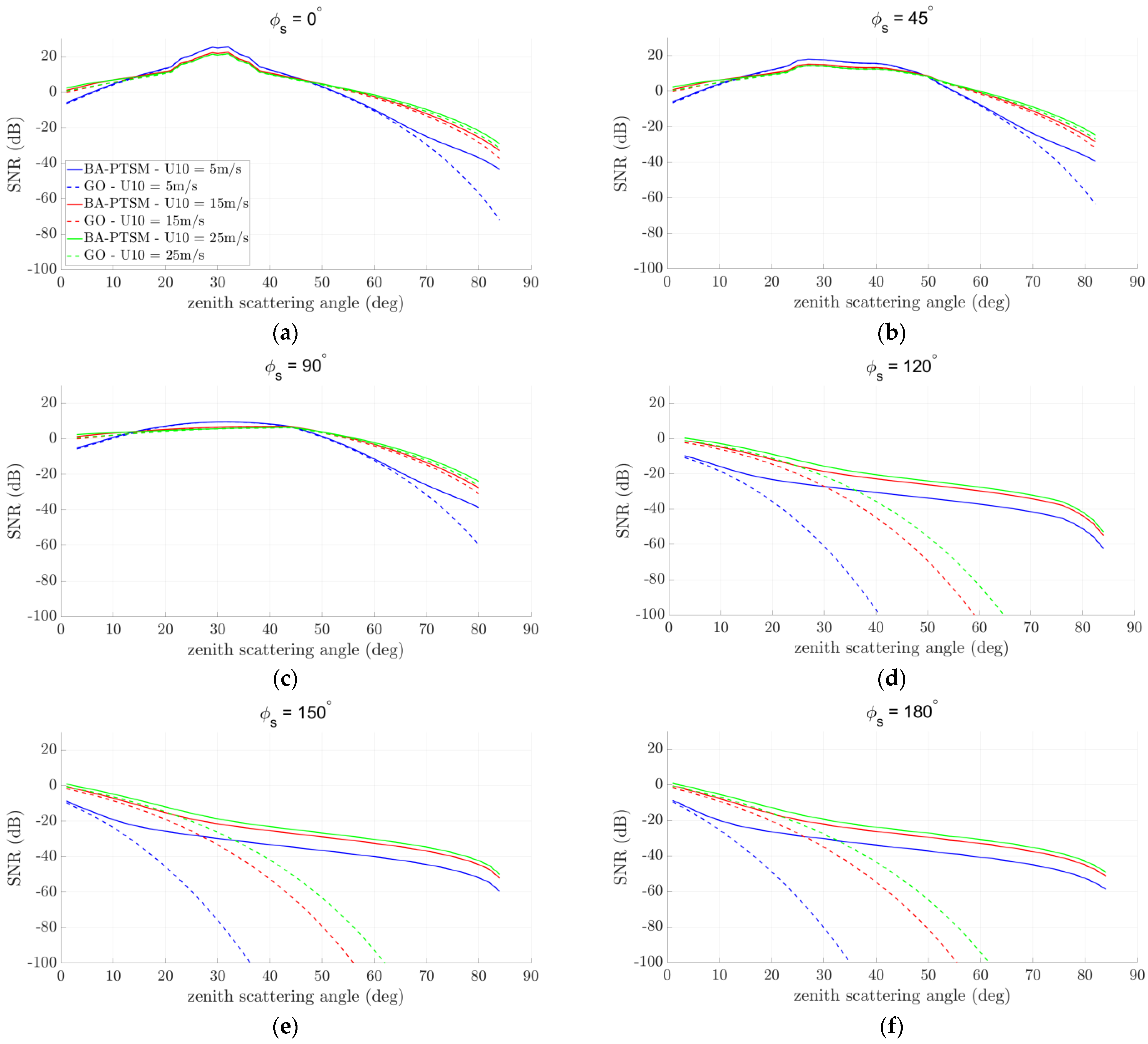
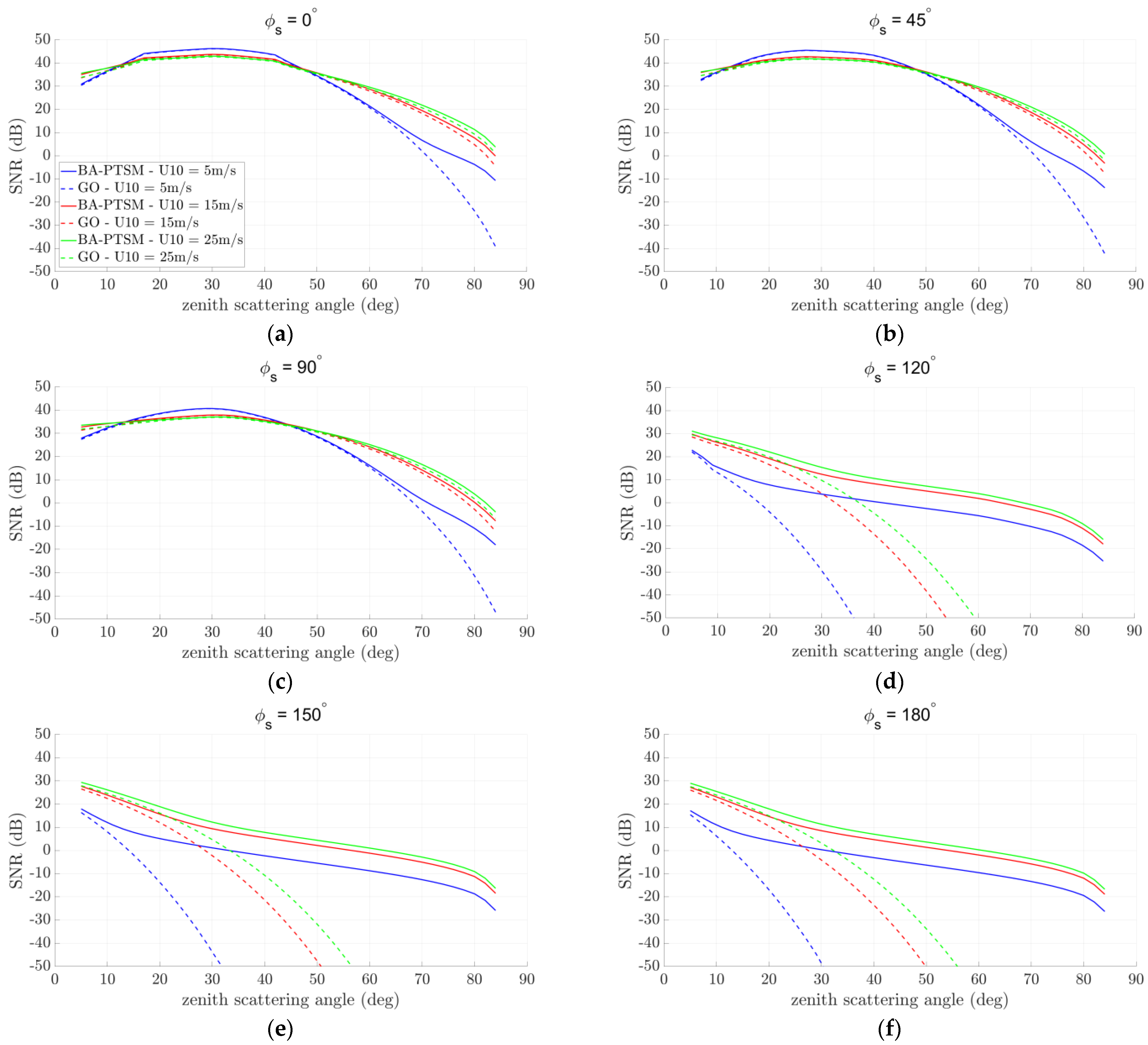
Figure 4 show the SNR for a spaceborne GNSS-R equipped with SGR-ReSi receiver and an LHCP and RHCP channel, respectively. Similarly,
Figure 5 and
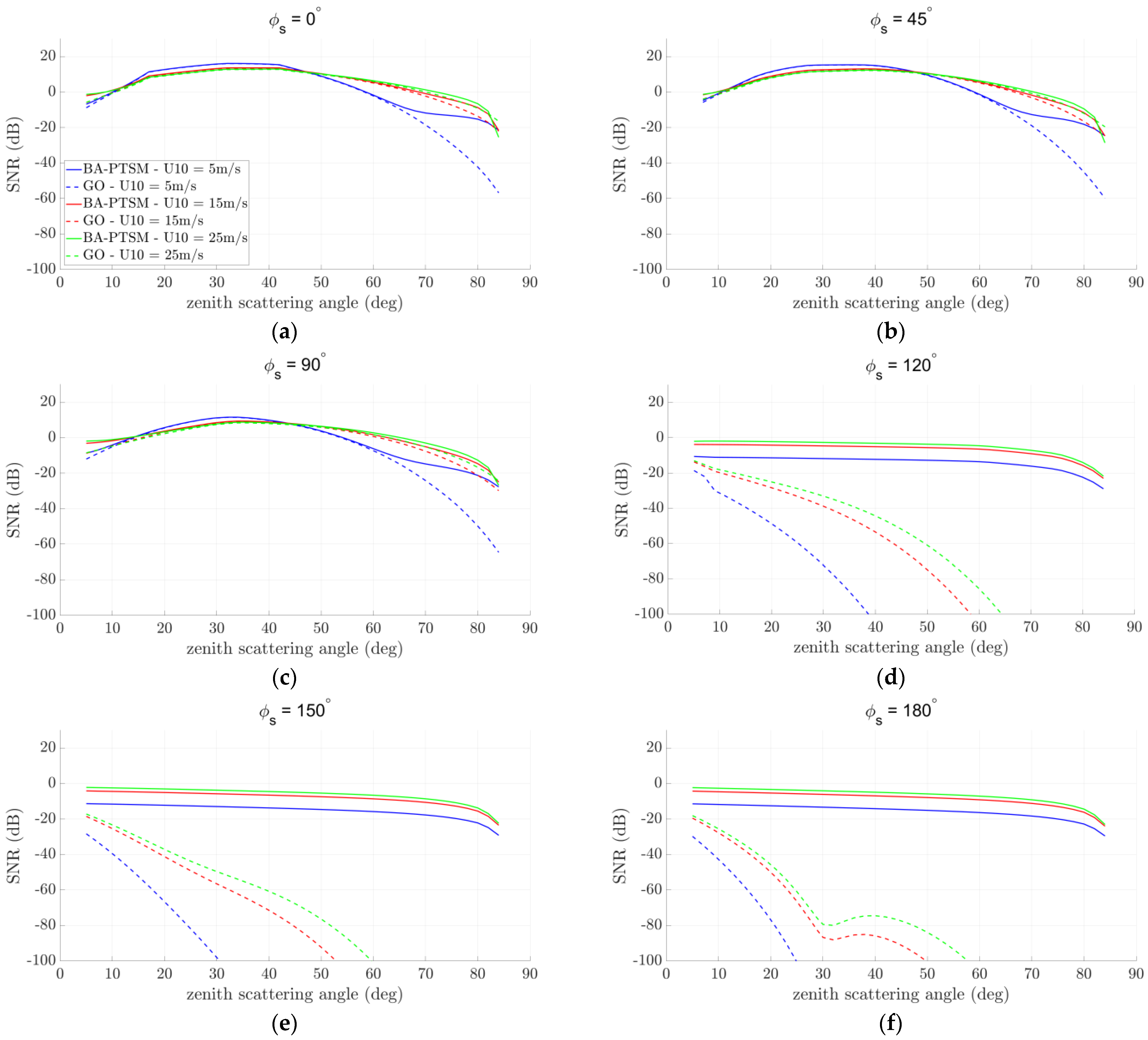
Figure 6 show results for an airborne GNSS-R equipped with a GOLD-RTR receiver and an LHCP and RHCP channel, respectively. For each scenario, SNR of the sea surface return is displayed as a function of the zenith scattering angle for different wind speeds-namely 5 m/s (gentle breeze, blue lines), 15 m/s (near gale, red lines), and 25 m/s (storm, green lines), and for different azimuth scattering angles, ranging from
(forward-scattering, where conventional GNSS-R operates) to
(back-scattering, where unconventional GNSS-R is conceived to work). For a more comprehensive analysis, results obtained with BA-PTSM (solid lines) are compared with classical GO model (dashed lines), wherein the same sea surface slopes PDF described in
Section 2 has been adopted for both scattering models. The evaluation of the sea scattering area has been accomplished by assuming the receiver along-track and across-track HPBW values reported in
Table 1.
Largest SNR values are reasonably obtained in the forward-scattering configuration and in the LHCP receive channel, regardless of sea state and receiver altitude. Indeed, this is due to a favorable combination of the following phenomena: first, sea surface geometry makes the impinging EM energy be largely reflected in a rather narrow angular region around the specular reflection direction, whose width increases with increasing wind speed; second, bistatic GNSS-R acquisition geometry is characterized by resolution cells whose sizes heavily depend on the delay-Doppler coordinates of the surface point and are largest at the specular reflection point. As a result, both sea surface NRCS and scattering area are largest in correspondence of the forward-scattering direction. Moreover, polarization inversion over seawater leads to an LHCP signal component larger than the RHCP one.
BA-PTSM better estimates the diffuse component of sea scattering at far-from-specular observation directions, i.e., for large
values or
not close to
, where GO severely underestimates sea surface NRCS due to the tangent plane approximation. Major differences between the two models can be appreciated for
, that includes the backscattering direction. In such configurations, the underestimation of the sea-reflected signal SNR is as large as several tens of dB for large zenith scattering angles regardless of sea state and receiver altitude, whereas for zenith scattering angles less than about
GO offers good accuracy in RL polarization, see
Figure 3f and
Figure 5f. Additionally, in far-from-specular directions, including backscattering, GO reveals less accurate in modeling the RR channel rather than the RL one. At the same time, as it was expected, BA-PTSM and GO provides very similar results at and around the specular direction, where small-scale roughness scattering is negligible compared to large-scale roughness scattering.
For the purposes of accurate simulation of GNSS-R signals, distinguished comments apply to the spaceborne and airborne scenarios. Indeed, for spaceborne GNSS-R equipped with an LHCP receiving channel (
Figure 3), it emerged that SNR is larger than 0 dB only in an angular region surrounding the specular direction, where GO and BA-PTSM provide very similar results. Conversely, departure of GO from BA-PTSM is significant at far-from-specular directions, specified by
or
. However, in such acquisition geometries, both scattering models predict SNR values well below 0 dB, and, then, the incoherently-averaged DDM would be dominated by thermal noise. Accordingly, accuracy of the scattering model in these acquisition geometries would not be an issue.
Spaceborne GNSS-R equipped with RHCP channel (
Figure 4) experiences SNR values well below 0 dB regardless of the acquisition geometry and sea state. Again, DDM products would be dominated by thermal noise and their simulation would be scarcely affected by the choice of the sea scattering model.
Finally, according to results shown in
Figure 3 and
Figure 4, accurate simulation of spaceborne GNSS-R signals over open sea can be carried out by relying on the classical GO model with anisotropic sea surface model. It is worth noting that, even assuming much larger coherent integration times (on the order of 100 ms or larger), GO might still be accurate enough for simulation purposes regardless of the acquisition geometry and sea state.
In the airborne scenario, the much lower receiver altitude with respect to spaceborne GNSS-R leads to much higher SNR values in all acquisition geometries and sea states, with LHCP channel providing larger signal strength compared to the RHCP one, see
Figure 5 and
Figure 6. SNR values as large as about 46 dB are obtained in the forward-scattering direction for low wind speed (
Figure 5). The much larger received signal strength calls for sea scattering models more accurate than GO, which is no longer reliable for proper simulation of sea-reflected GNSS signals. As a matter of fact, GO might lead to inaccurate results even for in-plane scattering (
Figure 5a), where for large
values and low wind speed, severe discrepancies between GO and BA-PTSM are visible. For out-of-plane scattering and in backscattering, GO becomes more and more inaccurate as
increases, i.e., as the scattering direction goes far from the specular one. As a result, application of GO is questionable for acquisition geometries specified by
, where GO would lead to severe underestimations of the sea clutter contribution.
Similar comments apply for simulation of the RHCP channel (
Figure 6), where GO offers limited applicability in far-from-specular directions. However, the reduced sea signal strength makes the application of GO less problematic especially for low wind speeds, see
Figure 6d–f.
5. Conclusions
In this paper, we presented an analysis of the SNR for the sea-reflected GNSS signal in arbitrary acquisition geometries, including the backscattering direction, which is of key relevance in maritime surveillance applications using GNSS-R. Sea surface scattering has been described by means of the recent BA-PTSM, that extends the original TSM to bistatic geometries and anisotropic random rough surfaces, such as sea surface, and provides analytical expressions for the polarimetric covariance matrix. BA-PTSM has the advantages of wider validity limits, especially with respect to GO, and accuracy comparable to other advanced scattering models, e.g., SSA2. For power budget analysis, standard GNSS-R processing chain, comprising coherent and incoherent integration steps, has been assumed and the sea surface signal strength has been evaluated at the output of the typical GNSS-R processing chain. Typical spaceborne and airborne GNSS-R receivers, namely SGR-ReSi and GOLD-RTR, respectively, have been considered. The sea scattering area has been evaluated by means of a numerical tool accounting for the receive antenna beamwidth and the actual configuration of iso-delay and iso-Doppler lines.
Numerical results comparing BA-PTSM with classical GO model have been presented for both spaceborne and airborne GNSS-R receivers and for both LHCP and RHCP receiving channels. It has been shown that for spaceborne GNSS-R, as long as standard GNSS-R processing chain is considered, GO can be safely adopted as the scattering model regardless of the polarization channel, acquisition geometry, and sea state. Conversely, for airborne GNSS-R simulation of sea surface, GO is accurate enough only in near-to-specular scattering directions, where SNR exhibits the largest values. In far-from-specular acquisition geometries more accurate scattering models, such as BA-PTSM, are required for a proper modeling and simulation of the sea surface return. Nevertheless, it should be noted that BA-PTSM reduces to GO at and around the specular reflection direction and, therefore, it could be used as the scattering model for fast and accurate simulation of GNSS-R signals reflected off sea surface regardless of the acquisition geometry, polarization, sea state, and receiver altitude.
Highlighted guidelines might be exploited for a fast and accurate simulation of sea-reflected GNSS signals in arbitrary acquisition geometries, which is an important preliminary task for a proper assessment of ship detection performance achievable with GNSS-R, also including unconventional imaging configurations. Further research works might focus on the evaluation and simulation of GNSS-R processing chains more suited to ship detection applications, such as bistatic SAR, as well as accurate link budget analysis for the ship target echo using advanced sea scattering models, such as BA-PTSM, for describing ship-sea EM interaction.


