Asymptotic Modeling of Three-Dimensional Radar Backscattering from Oil Slicks on Sea Surfaces

Abstract

This paper presents new results of a simulation of radar backscatter from oil slick areas on a real three-dimensional sea surface, based on a physical hydrodynamic model of surface wave damping in the presence of oil films, the local equilibrium model (MLB). To solve this problem, the modelling was carried out by using the first-order small-slope approximation (SSA1) model. It presents the advantage of having a very good compromise between rapidity and accuracy of the calculation. The choice of the model is justified by solving the two-dimensional problem with several asymptotic methods and further comparing the results with a rigorous numerical method, based on the Method of Moments (MoM). Two approaches called “thin-layer” (TL) and “classical” were used to deal with the double layer (air/oil/sea) problem. The TL approach assumes that this double-layer problem can be seen locally as a Fabry–Pérot interferometer, which implies that the Kirchhoff-tangent plane approximation (KA) is valid. The classical approach consists in neglecting the presence of the oil layer for dealing with electromagnetic backscattering, which is valid for very thin oil films compared to the electromagnetic (EM) wavelength. It is shown that these two approaches have rather complementary validity domains: The TL approach is always valid for small observation angles, which makes it suitable for near nadir sensors such as altimeters, whereas the classical approach is valid for moderate observation angles, which makes it suitable for most satellite applications. The 3D modelling results are compared with C-band and X-band measured data (CSK experiment and OOW NOFO experiment) in VV polarization. The calculation takes into account that the oil film on the sea surface is mainly in an emulsion state. The results highlighted the relevance of the MLB hydrodynamic model, as well as the SSA1 EM model combined wit the classical approach, for quantifying NRCS in seas contaminated with marine oil or surfactants. The agreement is indeed very good in the X-band range.

1. Introduction

Oil spill pollution detection has been the topic of investigation of a significant number of research papers, in particular by analyzing SAR data [1,2,3,4,5,6]. Fewer recent works such as [7,8,9,10,11,12] deals with quantitative electromagnetic (EM) modeling of sea oil spills. Most of this work focuses on homogeneous insoluble oil films on sea surfaces. Still, this restriction holds only for low-to-moderate winds, $u_{10}<$ 8–10 m/s, and for relatively young spills [3,13]. Fewer papers such as [7,10] deal with water-in-oil emulsions, which occur for moderate-to-high wind conditions and/or old spills. It is then of interest at least to study the influence of oil emulsification on the electromagnetic scattering, as we often lack of information on the characteristics of an observed oil slick at sea.

Besides, in order to better understand and to thoroughly analyze and interpret radar measurement data, it is necessary to develop accurate models of radar backscattering from both clean and contaminated seas, that are based on a realistic hydrodynamic modeling. Thus, two important conditions must be fulfilled: first, the hydrodynamic modeling must be able to take into account the specific characteristics mineral of oil slicks on the sea surface; second, the electromagnetic modeling must be able to handle the multi-scale feature of the sea-like surface. Concerning the first condition, the Elfouhaily et al. spectrum [14] is well-known and widely used for describing the clean sea surface heights. The presence of an oil slick on the surface of the sea is known to strongly damp the capillary waves of the spectrum. This phenomenon is usually called the Marangoni damping [15]. Nevertheless, this damping model does not depend on the film thickness and is then limited to very thin films [16]. It is also uneasy to relate its input parameters to the physical characteristics of the marine oil film. It is then more appropriate to use a refined model, provided that we are able to determine its parameters suitably. That is why the model of local balance (MLB) [17] is chosen here, following our experience of previous work [16,18]. Concerning the second condition, as a general consideration for dealing with a multi-scale surface, the electromagnetic model should also be multi-scale, at least if we want to use the same model for different configurations (like small and large angles, in particular). Then, the classical GO (Geometric Optics) and SPM (Small Pertubation Method) models cannot fill this condition alone for this purpose. Thus, a so-called unified should rather be elected. Among these models, the first that has been developed is the two-scale model (TSM). Since then, a number of refined asymptotic electromagnetic models commonly used for sea-like surfaces have been developed (SSA1, WCA, LCA, …) [19,20,21].

This paper presents an extension of previous work [16] to three-dimensional (3D) problems with validations with measurements, by using two asymptotic models for dealing with the case of oil slicks on sea surfaces: the approaches called “thin-layer” (TL) and “classical”. The TL approach, that has been proposed by some of the authors [16], assumes that this double-layer (air/oil/sea) problem can be seen locally as a Fabry–Pérot interferometer, which implies to assume that the Kirchhoff-tangent approximation (KA), is valid. In addition, the two air/oil and oil/sea interfaces are assumed to be identical and parallel, which is valid for thin enough oil films, giving its name to this approach. By comparison, the classical approach consists in neglecting the presence of the oil layer for dealing with electromagnetic backscattering, which is valid for infinitely thin oil films compared to the EM wavelength. It is the approach that is usually used in the literature for modeling oil films on the sea surface; yet, to our knowledge, the validity of this assumption had not been analyzed in details before.

These two approaches are first analyzed in details numerically by comparison with a reference numerical method based on the Method of Moments (MoM) for two-dimensional (2D) problems in Section 3 and Section 4, where the influence of emulsification is analyzed in Section 3 before analyzing the accuracy of asymptotic EM models in Section 4. We would like to insist on the originality of this work, where both the refined hydrodynamic MLB model is applied, which provides realistic hydrodynamic simulations when combined the Elfouhaily et al. spectrum, and the validity of both the classical and the TL approaches are compared and validated. The classical approach only is generally used without detailed quantitative validation [22]. Besides, several asymptotic EM models are applied and validated here, whereas generally only the SPM1 (Bragg scattering) is applied [22,23,24]. Recent works [4,12,22,25,26] considered unified EM methods (most of the time, the tilted Bragg or two-scale model—TSM), but they are usually based on a more simple and less adapted damping model (usually, the Marangoni damping model [15]), and are not validated for the specific case of oil slicks. The two TL and classical approaches are then compared in 3D with in-field measurements in Section 5, by analyzing two distinct measurement campaigns: the CSK experimental data in the French coasts, and the OOW NOFO experiment off Bergen, Finland. Comparing the classical GO and SPM models with the unified SSA1 model makes it possible to highlight the limitations of the former two models, showing in particular that the widely used Bragg scattering model is not always enough to describe the scattering mechanisms.

We will see in the following that, in general, these two approaches have rather complementary validity domains: The TL approach is always valid for small observation angles, which makes it suitable for near nadir sensors such as altimeters, whereas the classical approach is valid for moderate observation angles, which makes it suitable for most satellite applications. The study of the influence of different physical parameters was conducted (the observation angle, the frequency, and the oil viscosity); it was found to be in qualitative agreement with previous work applied to measurements [27] (see chapter 2 and references therein).

Thus, these two simplifying approaches make it possible to develop 3D models of radar backscattering from both clean and contaminated seas by using asymptotic analytical models adapted to sea-like surfaces, such as the two-scale model, the small slope approximation (SSA), and the weighted curvature approximation (WCA) [19]. This work presents such developments and further validates these models by comparison with measurements. Before detailing the analysis, next section summarizes the methodology used here for calculating the scattering from clean and contaminated seas.

2. Methods and Data Sources

2.1. Methods

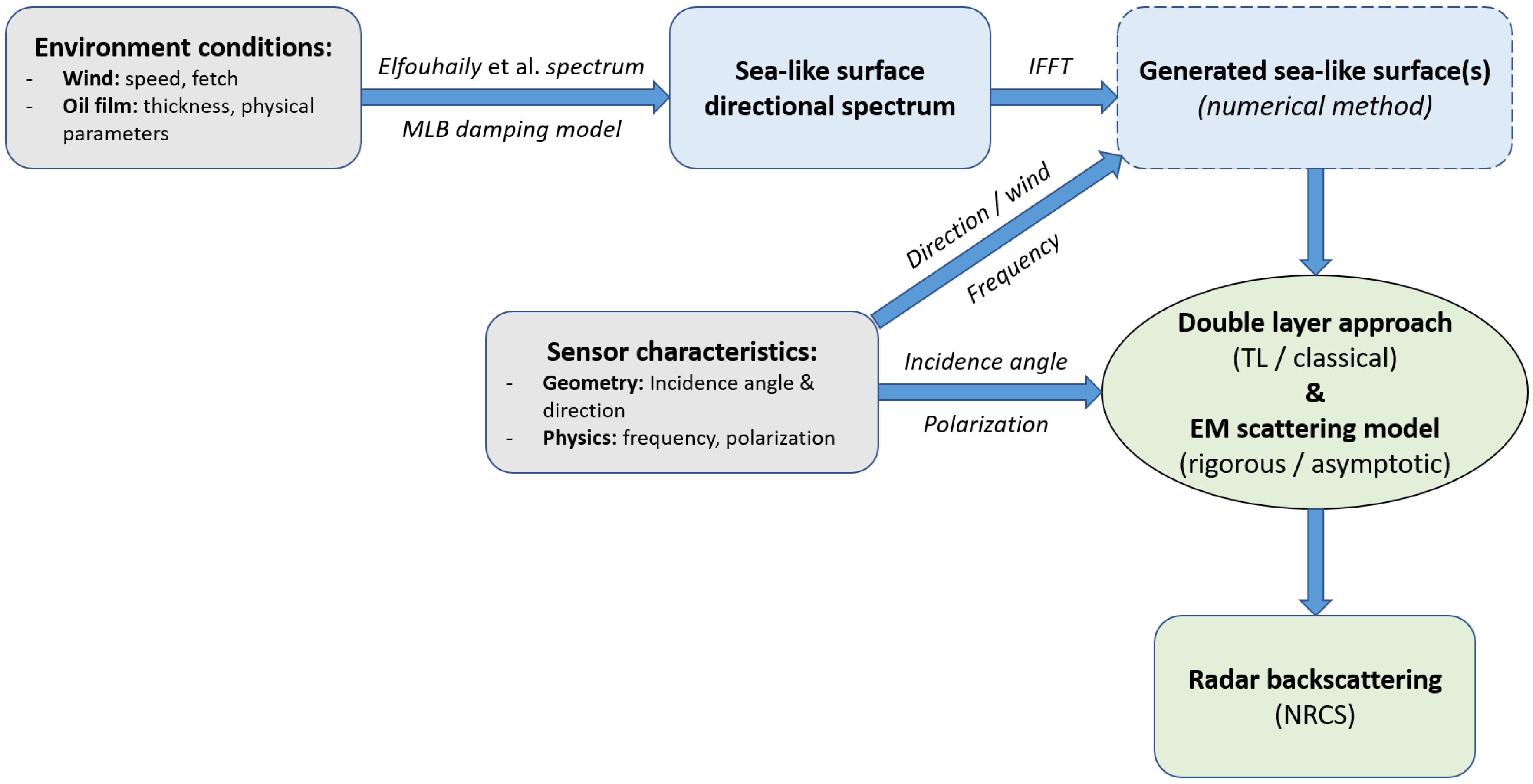
This section is devoted to giving the main methodology for calculating the electromagnetic wave scattering from both clean and contaminated seas, as summarized in Figure 1. The main steps may be summarized as follows:

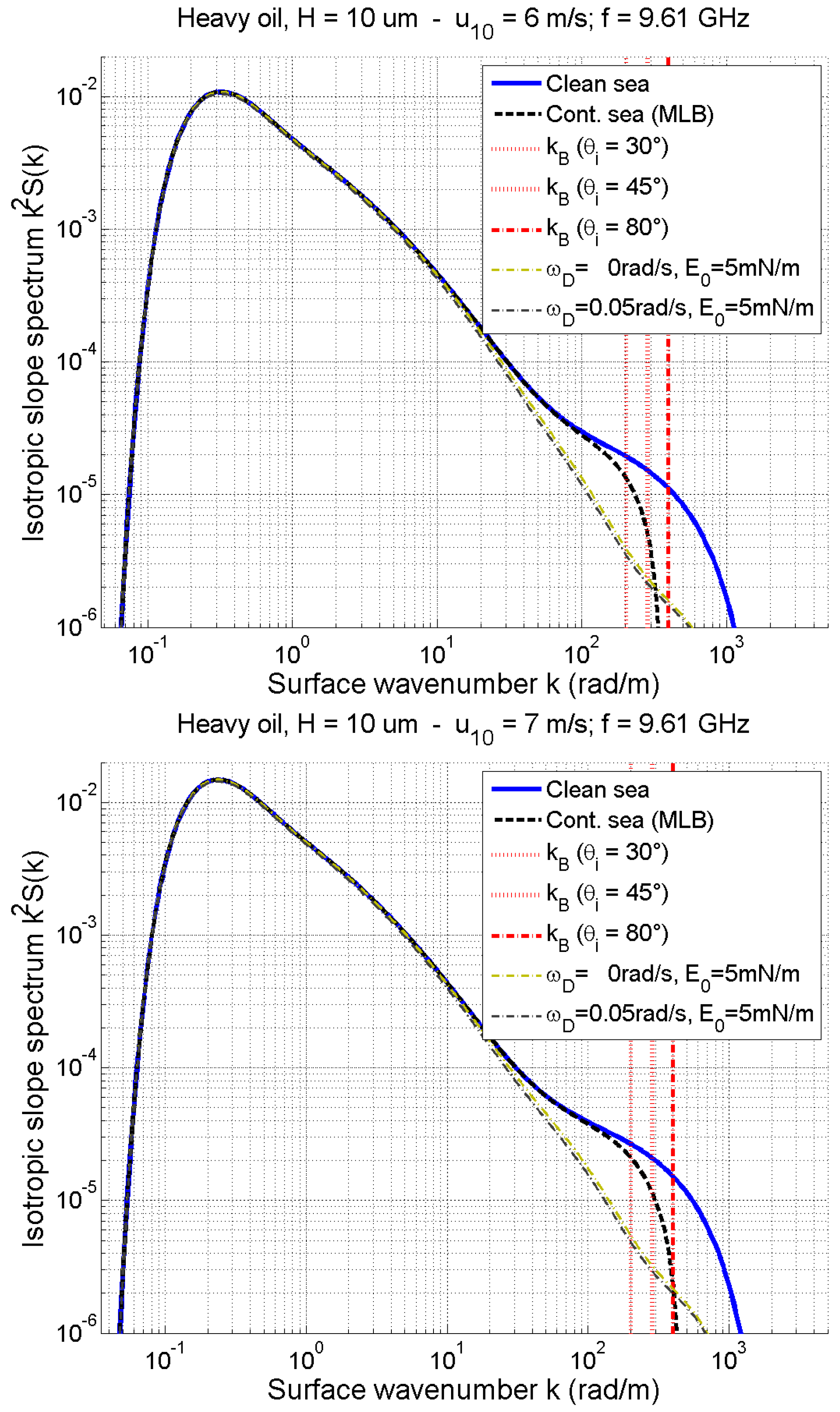
• The sea-like surface spectrum is defined with respect to the environment conditions, by using the Elfouhaily et al. spectrum model for the clean sea surface; for the case of oil films, the MLB model is used to model the surface spectrum damping.
• For the case of numerical EM methods, sea-like surfaces must be generated from the directional spectrum by IFFT (Inverse Fast Fourier Transform), given the frequency of the sensor and its azimuth direction with respect to the wind direction (in addition to the environment condition parameters).
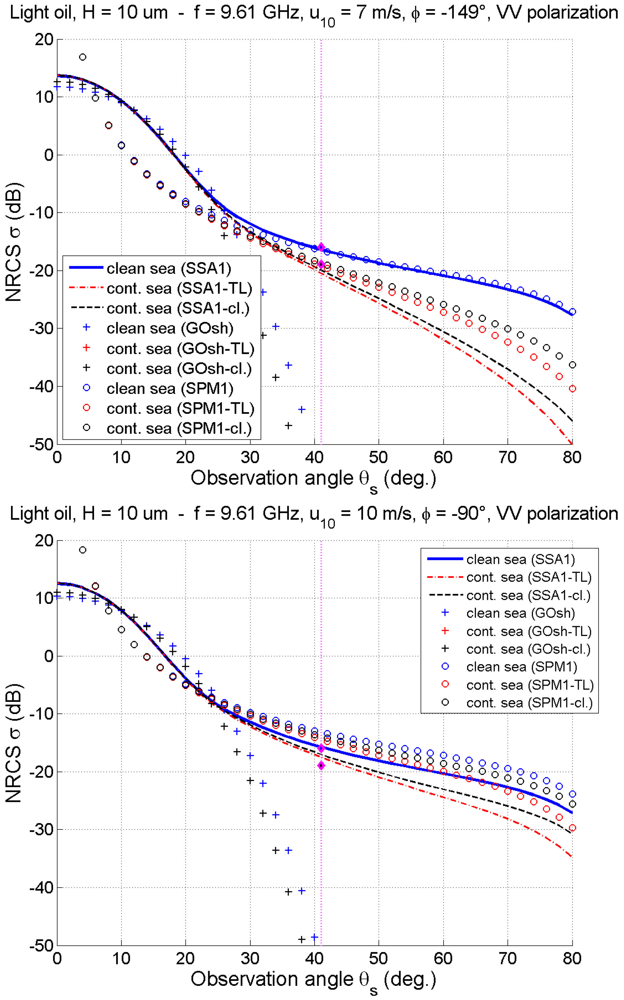
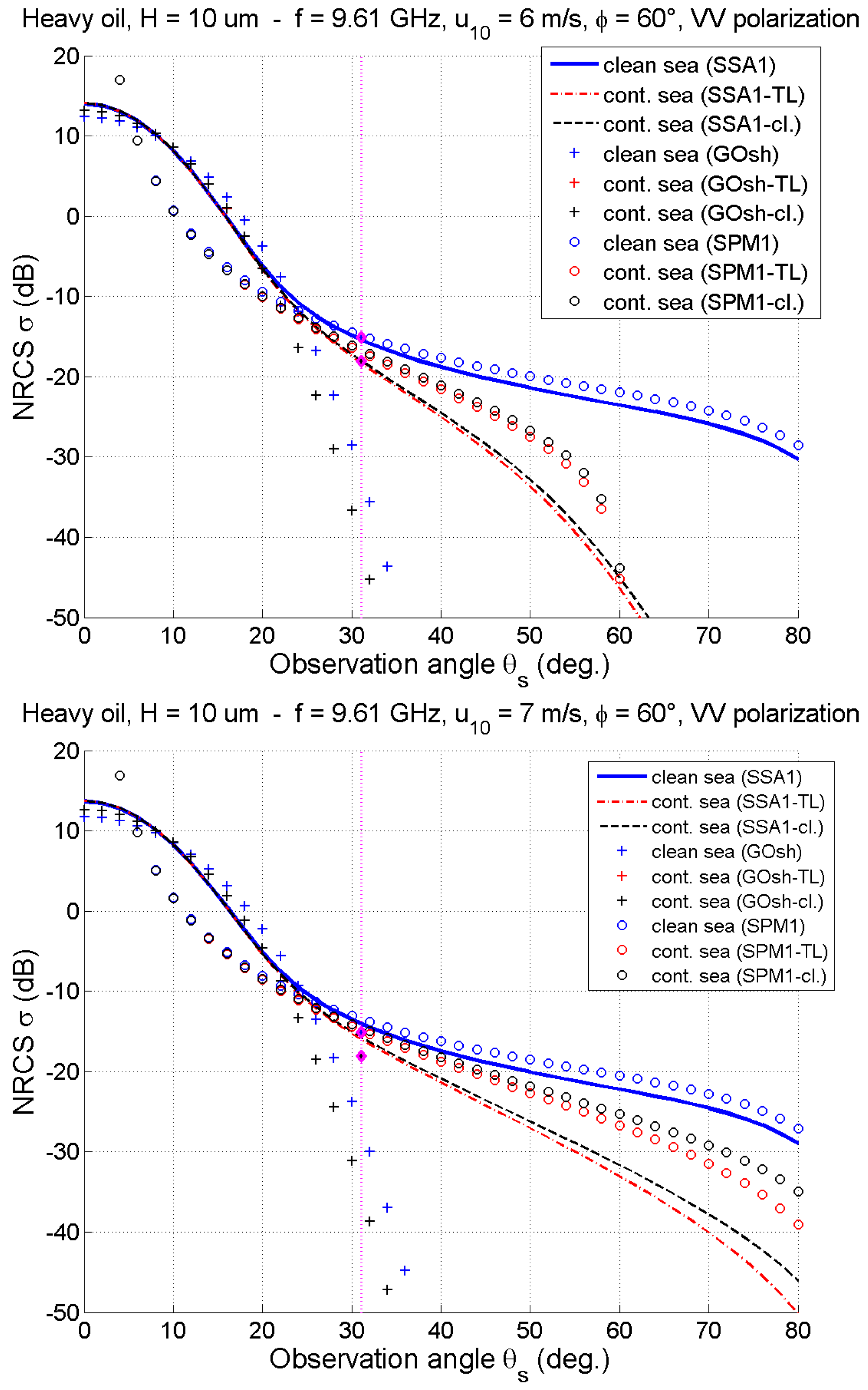
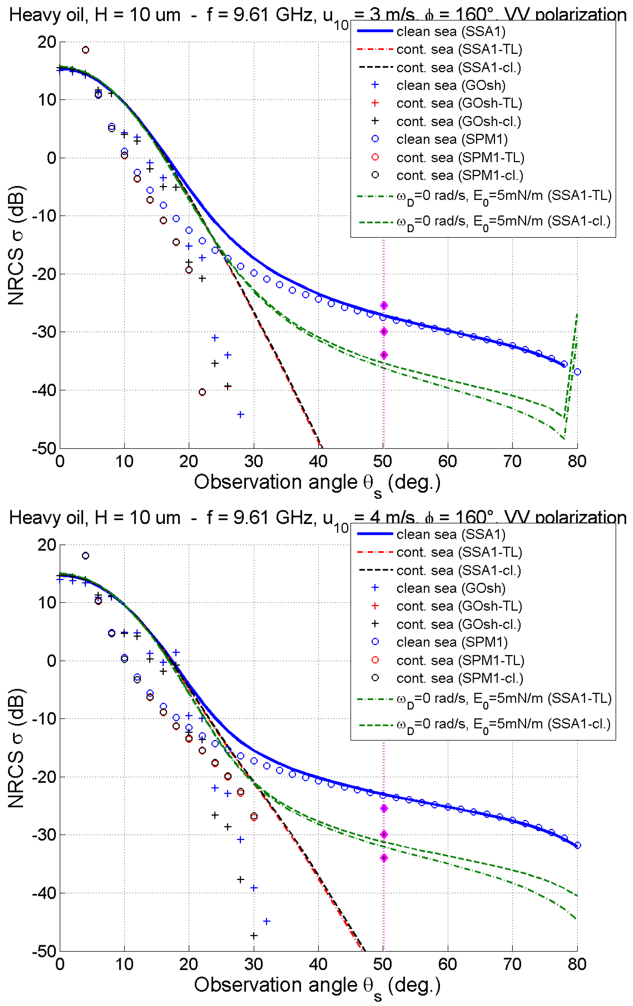
• A simplifying approach for reducing the double layer (air/oil and oil/sea) problem to a single interface problem is elected; then, to deal with the latter problem, an appropriate electromagnetic model is applied. The simplifying approach is either the “thin-layer” (TL) or the classical approach; the EM scattering model may be either rigorous (based on the Method of Moments, MoM) or asymptotic (in particular, the SSA1). This makes it possible to calculate the scattered wave, and in particular, the backscattered intensity (NRCS, Normalized Radar Cross Section).

2.2. Data Sources

Two data sets have been used here to validate the proposed electromagnetic methods developed in the paper. The first data set corresponds to COSMO-SkyMed data that have been acquired in February–March 2011 around the French coast, for which the radar works at $9.61$ GHz in $\mathrm{VV}$ polarization. Out of the 20 images available, oil spills have been detected in 3 images. These 3 case studies (scenarios) are:

1.

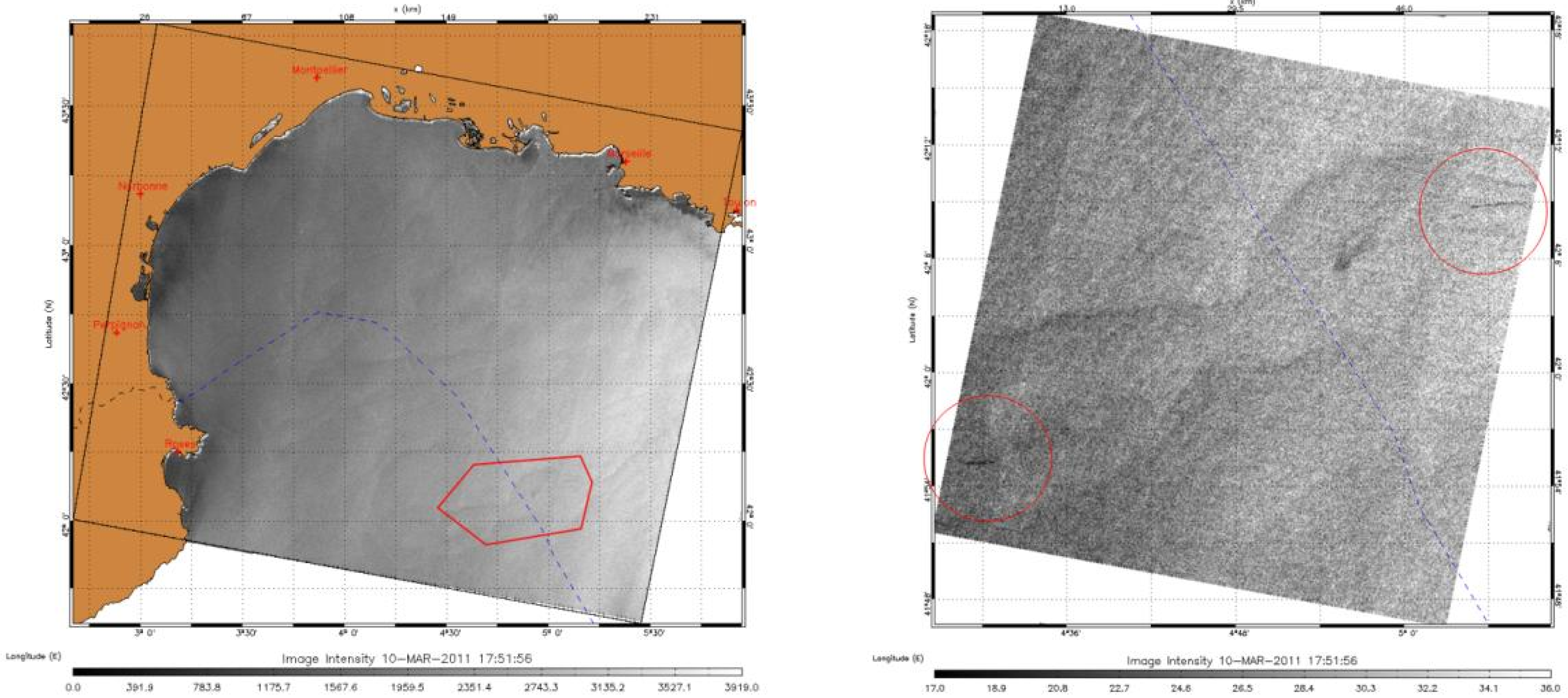
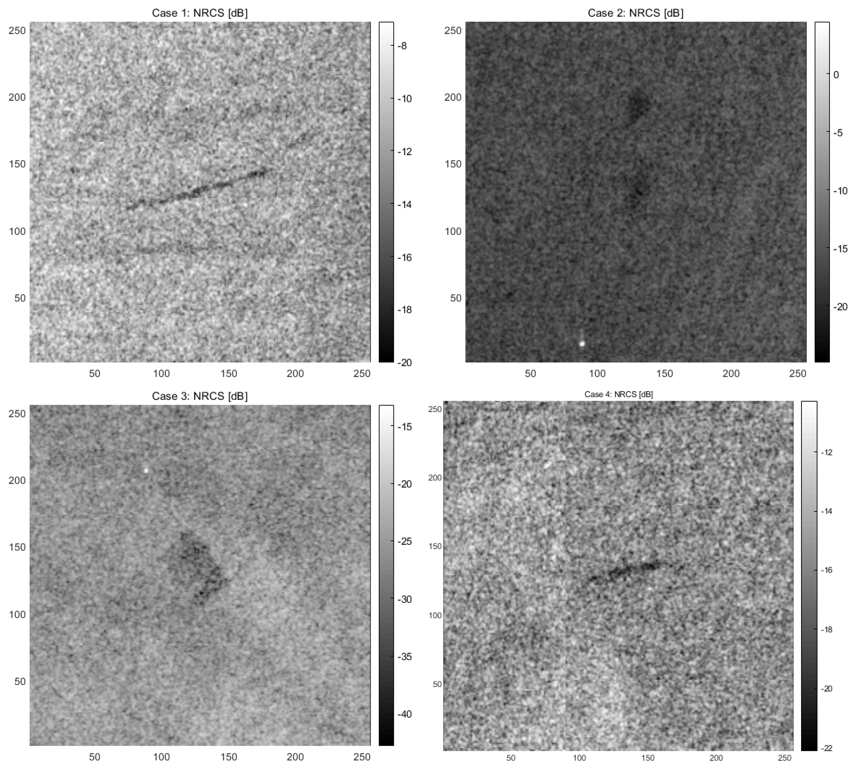
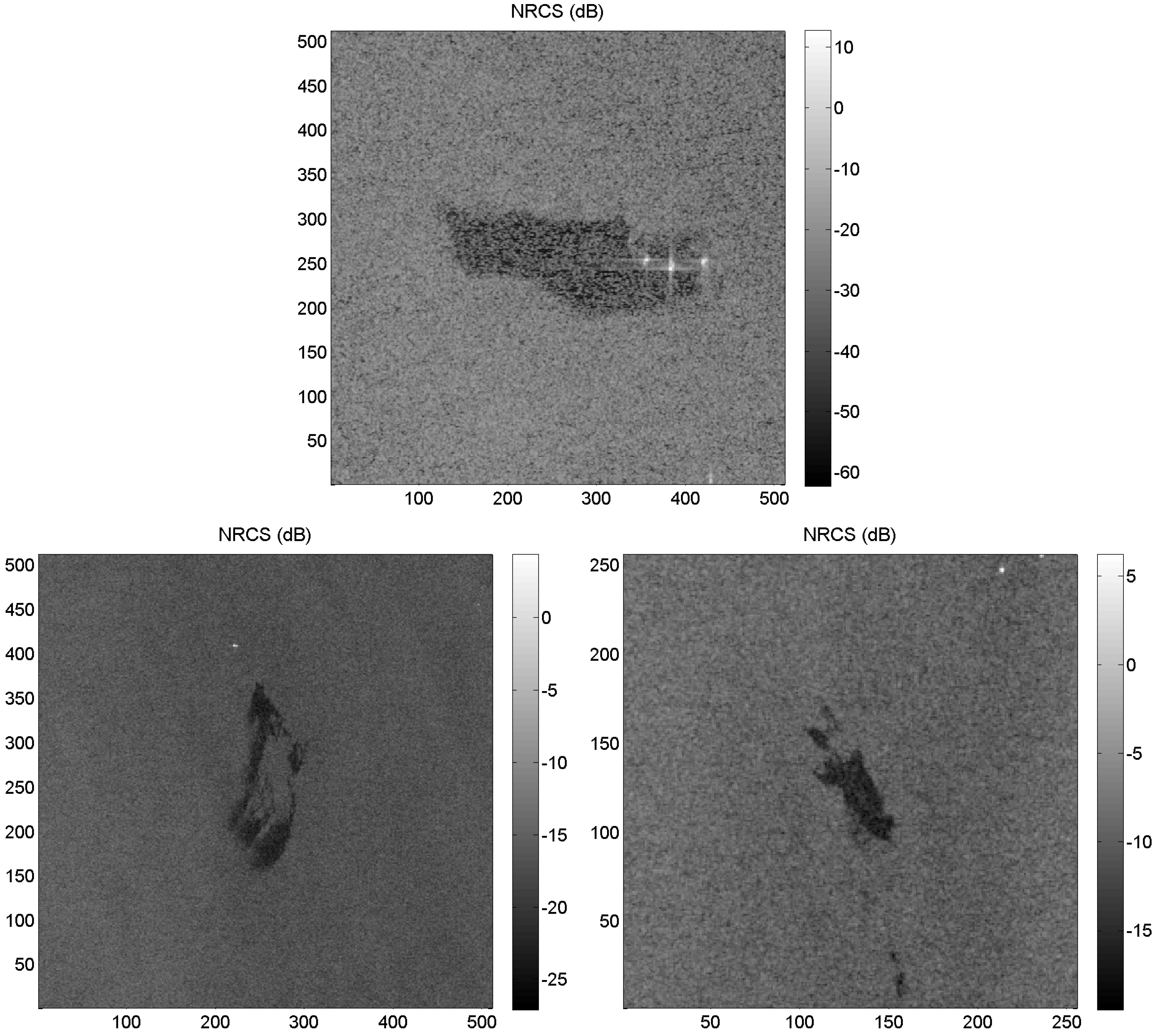
The first case study concerns the images in Figure 2, taken on 10 March 2011, 17 h 51${}^{\prime }$. Two areas are concerned by potential oil spills: the Western one (area about $0.96$ km${}^2$–length $3.15$ km) and the Eastern one (area $1.39$ km${}^2$–length $5.64$ km). The incidence angle is equal to about ${27}^{°}$ and ${31}^{°}$ for the South West and North East cases, respectively. The average estimated wind speed is $u_{10}=6.3$ m/s and $u_{10}=6.4$ m/s, respectively. Note that, in Section 5.1, the Western area will be considered and referred to as scenario 1, whereas the Eastern area will be considered and referred to as scenario 4.

2.

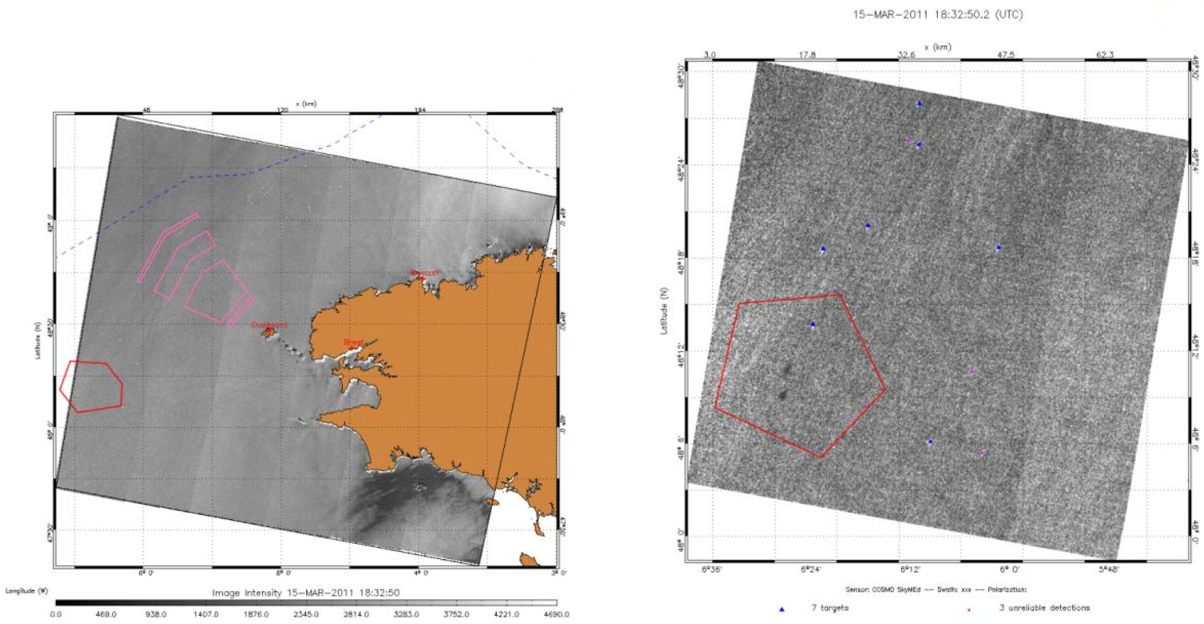
The second case study concerns the images in Figure 3, taken on 15 March 2011, 18 h 32${}^{\prime }$. One area is concerned by 2 potential oil spills: the Northern one (area about $0.78$ km${}^2$–length $1.82$ km) and the Southern one (area about $0.98$ km${}^2$, length $1.38$ km). The incidence angle is equal to $40.9^{°}$ in this area. The average estimated wind speed is $u_{10}=10.4$ m/s. Note that, in Section 5.1, only the Southern area will be considered and referred to as scenario 2.

3.

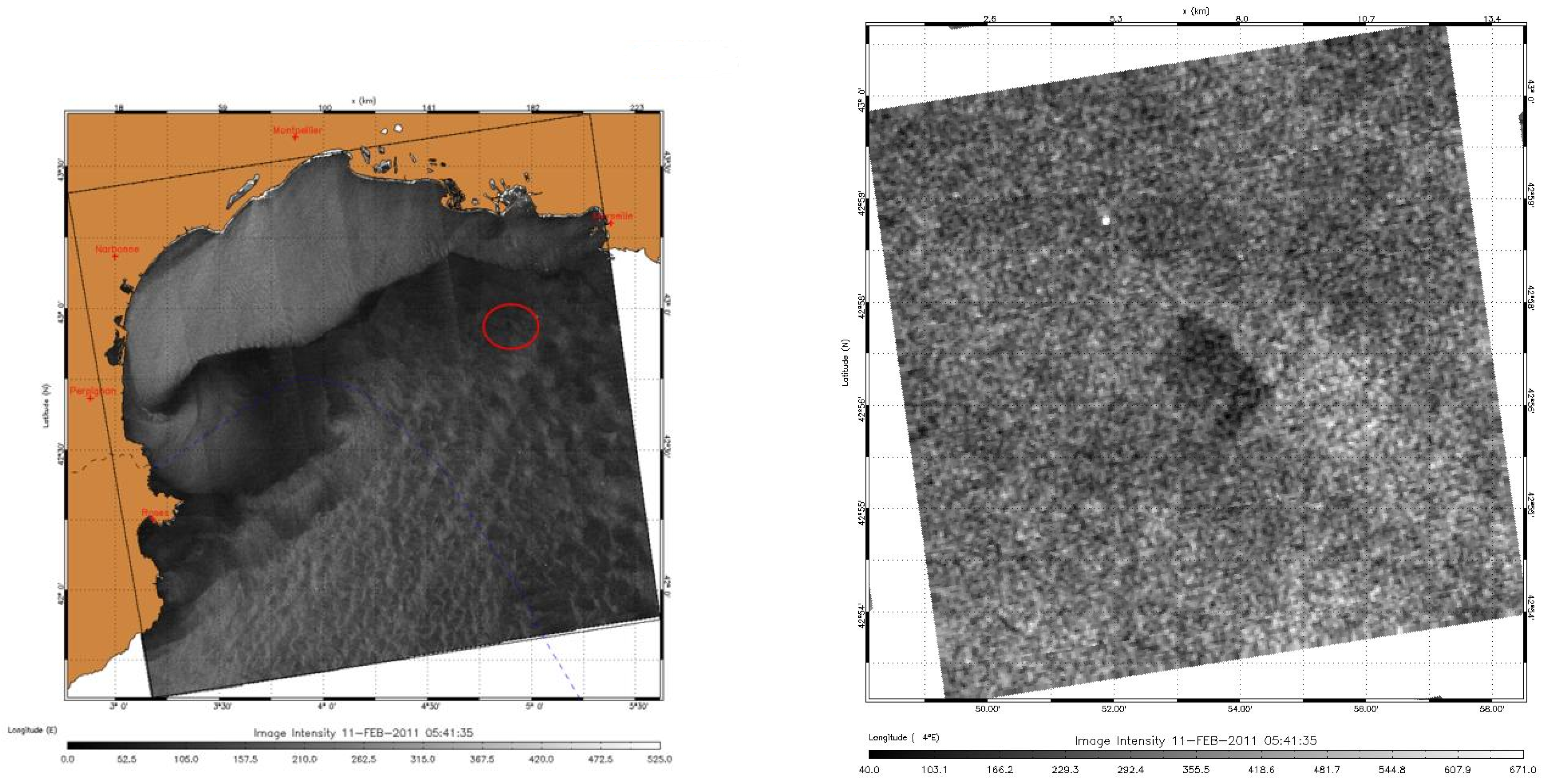
The third case study concerns the images in Figure 4, taken on 11 February 2011, 5 h 41${}^{\prime }$. One area is concerned by 1 potential oil spill: area about $3.42$ km${}^2$–width $2.67$ km. The incidence angle is equal to $50.9^{°}$ in this area. The average estimated wind speed is $u_{10}=2.5$ m/s. Note that, in Section 5.1, this area will be referred to as scenario 3.

All these 3 images correspond to CSK data in Huge Region mode, with a spatial spacing (pixel resolution) of 100 m.

The second data set corresponds to measurements that have been acquired during the oil pollution experiment called oil-on-water (OOW) NOFO exercise [28] in June 2011 off Bergen (Finland). In this context, 3 images of interest have been retained. They are all in $\mathrm{VV}$ polarization. These 3 case studies (scenarios) are:

1.

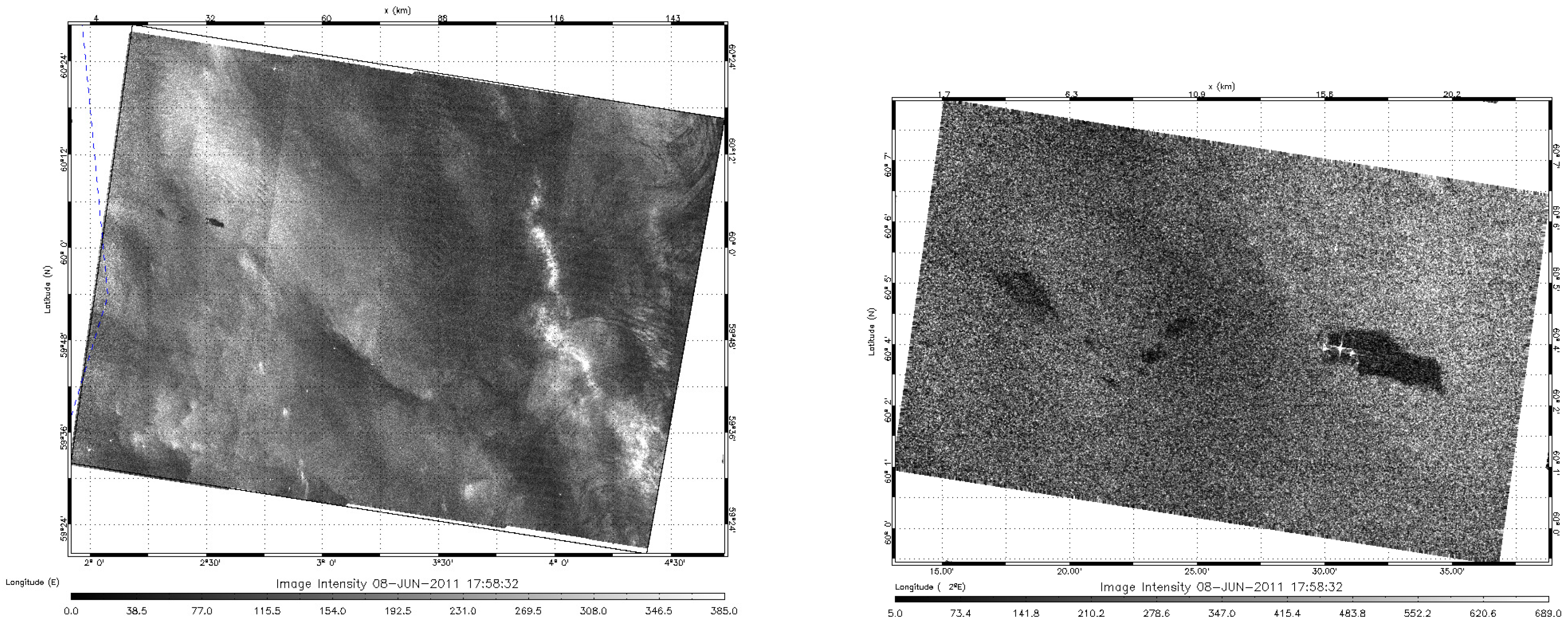
The first case study concerns the images in Figure 5, taken on 8 June 2011, 17 h 58${}^{\prime }$. It is a ScanSAR Wide (X band) image in VV polarization. The incidence angle is equal to about ${48}^{°}$ in the area of the pollution, where the average estimated wind speed is $u_{10}=2.6$ m/s.

2.

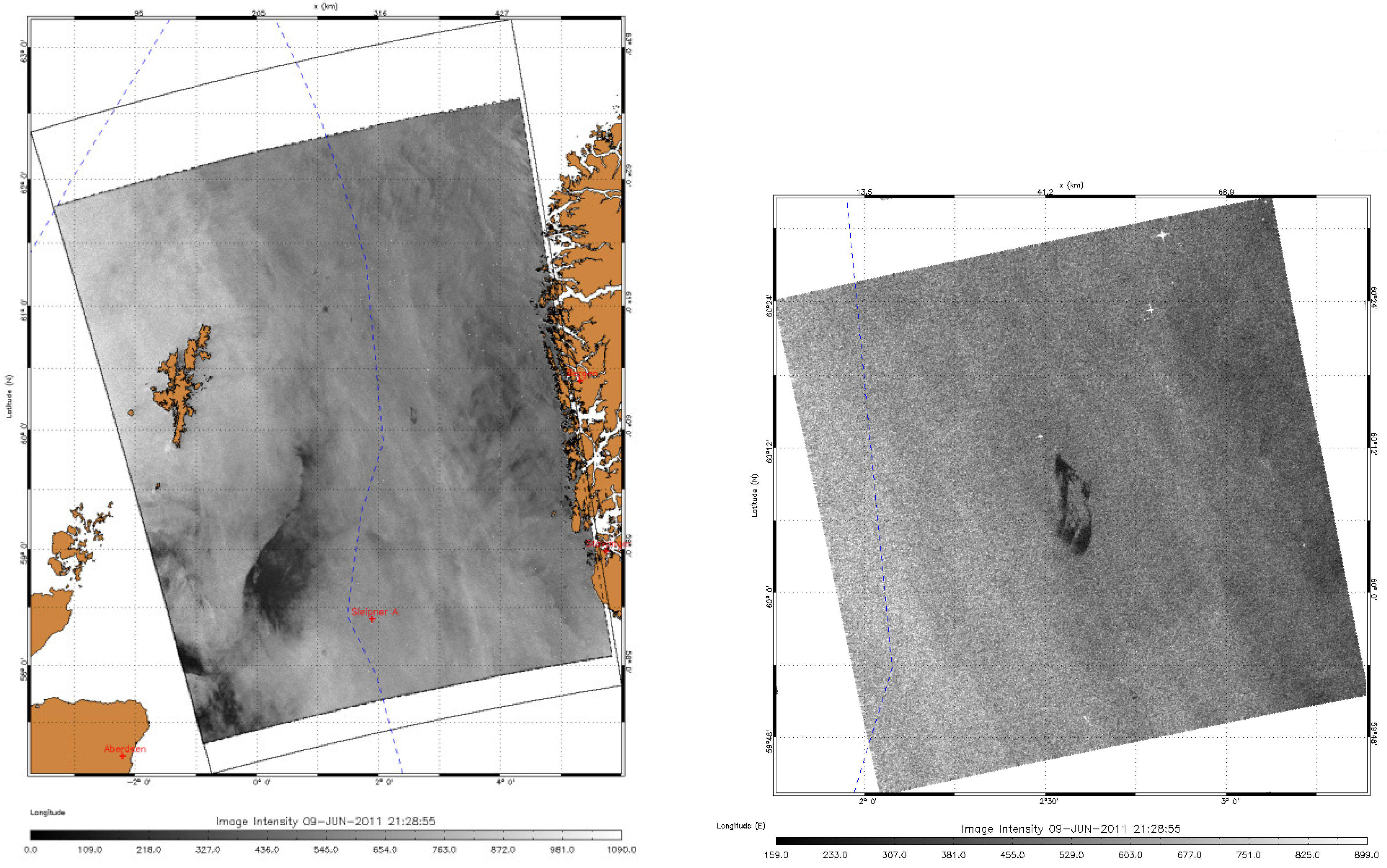
The second case study concerns the images in Figure 6, taken on 9 June 2011, 21 h 28${}^{\prime }$. It is an ASAR/ENVISAT (C band) image in VV polarization. The incidence angle is equal to about ${34}^{°}$ in the area of the pollution, where the average estimated wind speed is $u_{10}=4.5$ m/s.

3.

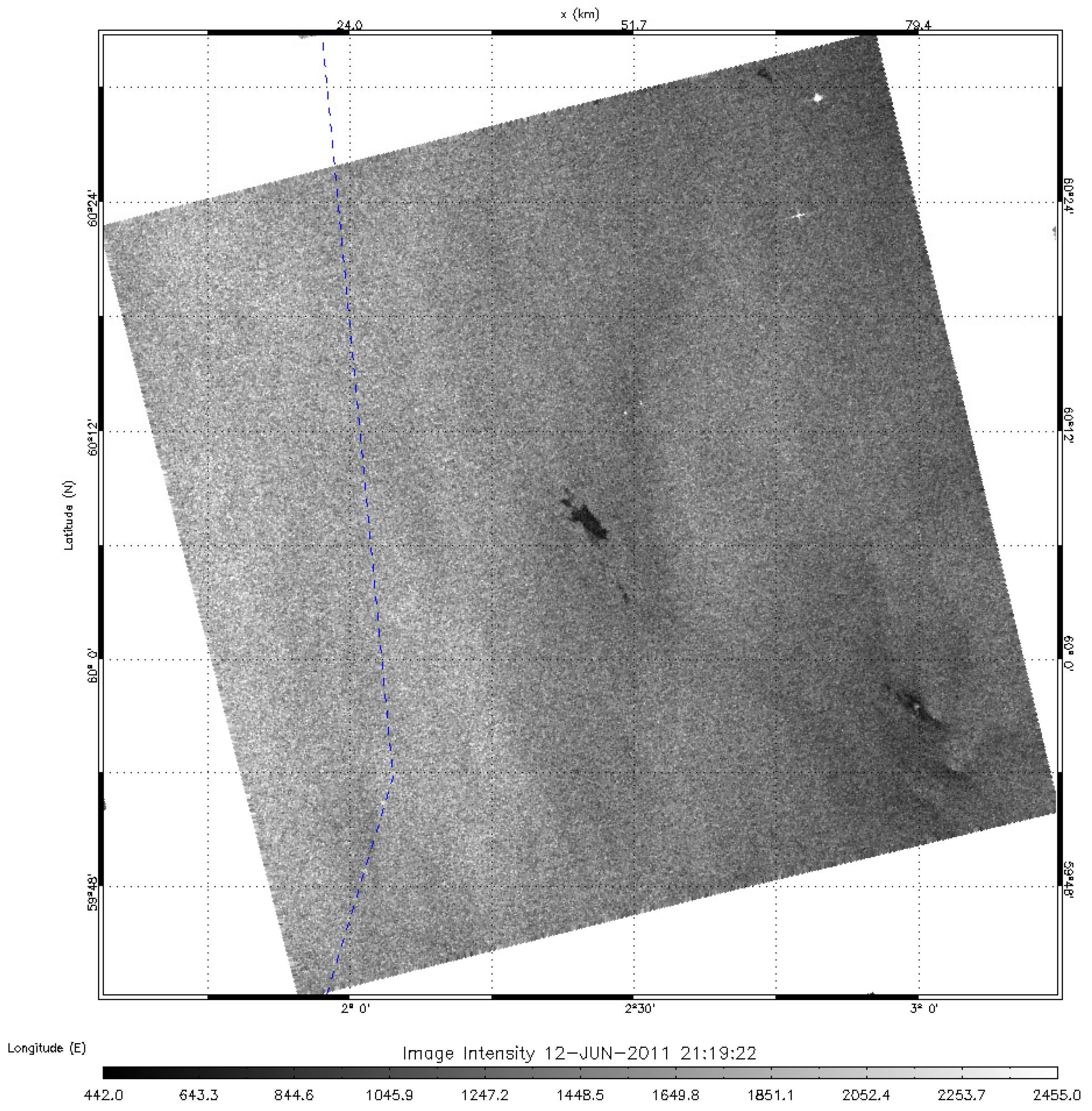
The third case study concerns the images in Figure 7, taken on 12 June 2011, 21 h 18${}^{\prime }$. It is an ASAR/ENVISAT (C band) image in VV polarization. The incidence angle is equal to about ${25}^{°}$ in the area of the pollution, where the average estimated wind speed is $u_{10}=5.8$ m/s.

The first case corresponds to CSK data in Wide Region mode, with a spatial spacing (pixel resolution) of 30 m. Cases 2 and 3 correspond to ASAR/ENVISAT data in Wide Swath Medium Resolution mode, with a spatial spacing (pixel resolution) of 75 m.

3. Influence of Emulsification

For comparing simulations with measurements at sea, the oil weathering effect should be taken into account in the numerical simulations in order to make comparisons with the same physical conditions. The main phenomena that must be taken into account are: evaporation, precipitation, aging, and emulsification. The first two phenomena can mainly be handled by a reduction of the quantity of floating oil. Aging induces an increase of the oil viscosity, as discussed further in the paper. Last, emulsification implies that the oil film changes from a homogeneous film to an inhomogeneous one, which becomes an oil-in-water emulsion at the surface of the seawater; but at typical radar frequencies (at least up to X-band), given the geometrical dimensions of the emulsion, this may be handled by considering an equivalent relative permittivity [10].

Here, we study the influence of the phenomenon of oil emulsification on the electromagnetic response of a contaminated sea, by comparison with a clean sea. Indeed, after the oil damping at sea, as time goes by, the homogeneous oil film at the sea surface is subject to several degradation phenomena, including emulsification with the sea water, which is mainly due to the surface agitation. This phenomenon is all the faster as the wind speed $u_{10}$ is high. Thus, for a given oil slick pollution, the emulsification effect should be taken into account in general in the electromagnetic modeling, or at least its influence on the radar backscattering must be studied.

For these simulations with emulsified oil, we need to know the equivalent relative permittivity of this mixture of emulsified oil in seawater. To do so, we based our work on the PhD thesis of Lamkaouchi [29] which made it possible to measure the equivalent relative permittivity of a mixture of oil with fresh water in different proportions, for frequencies $3.6$ GHz, $9.45$ GHz, and $15.48$ GHz. In order to make a comparison with the scenario 4 (with a frequency of 10 GHz) in [16], we took an intermediate value of $50\%$ of oil for $50\%$ of fresh water. This configuration is also close to a measurement scenario to be shown in the following of the paper, at $f=9.45$ GHz. Measured equivalent relative permittivity was ${ϵ}_{r2}^{eq}=13+2i$ [29]. Knowing that the relative permittivity of seawater is greater than that of fresh water at this frequency, this corresponds to a mixture of about $45\%$ of oil for $55\%$ of sea water. Thus, the numerical simulations are led for a contaminated sea with ${ϵ}_{r2}^{eq}=17+4i$, on the scenario 4 of [16], by considering light oil with viscosity ${\nu }_{oil}=0.1$ cm${}^2$/s.

Besides, following [16], we highlight that the rigorous numerical method which is used for the validations for 2D problems in this paper (Section 3 and Section 4) is based on the method of moments (MoM). Still, a direct LU inversion would be too much time consuming, that is why acceleration algorithms have been applied. For the single interface scattering numerical computations (clean sea, cont. sea combined with either the TL or the cl. approach), the FB (Forward–Backward) method [30] combined with SA (Spectral Acceleration) [31] is applied. Moreover, for the double (air/oil/sea) layer problem (that is, the cont. sea calculated rigorously), the PILE method [32] with FB-SA is applied. The parameters of the FB-SA are collected in Table 1 of [16] and more information may be found in the surrounding text.

The associated numerical results are plotted in Figure 8. It can be seen that the results are close to the homogeneous oil in Figure 11 of [16].

The rigorous calculation of the contaminated sea shows a slight decrease of the NRCS from homogeneous oil to emulsified oil; this decrease is enhanced when the observation angle ${\theta }_s$ increases. The so-called “classical” approach gives exactly the same result for both cases, which implies that it gives a slightly poorer agreement here with the rigorous method for moderate angles. By contrast, the so-called “thin-layer” (denoted as TL) approach shows a slight increase of the NRCS with increasing ${\theta }_s$. Thus, it underestimates the NRCS only slightly, making this approximation valid up to about ${40}^{°}$ (with $\approx 2$ dB difference criterion). Recall that the ratio values for ${\theta }_s\gtrsim {50}^{°}$ are not reliable, because the NRCS levels become negligible.

Thus, oil emulsification does not significantly modify the qualitative and quantitative analyses led in previous work [16]. We can conclude that the main influence of this phenomenon is a slight decrease of the reference NRCS, and that the validity domain of the TL approach is extended to higher observation angles ${\theta }_s$. Then, it is appropriate to extend now this approach to 3D problems in order to make comparisons with measurements.

4. From 2D Problems to 3D Problems

The rigorous computations led in [16] and in Section 3 of this paper, which though consider two-dimensional (2D) problems, are already rather extensive in memory space and computing time. Thus, it is not possible to extend these computations to three-dimensional (3D) problems. That is why we are going to apply several asymptotic electromagnetic models commonly used for sea-like surfaces (SSA1, WCA, LCA, … [19]) for 2D simulations and extend them to 3D problems. Their validity domains are well-known for clean seas for both 2D and 3D problems. The following 2D simulations will make it possible to check if these models are still valid for contaminated seas, and to study if their validity domains are modified.

Then, the asymptotic electromagnetic model which will be chosen for dealing with both clean and contaminated seas will be extended to the 3D case. A comparison of this model with measurement results will then be led in Section 5.

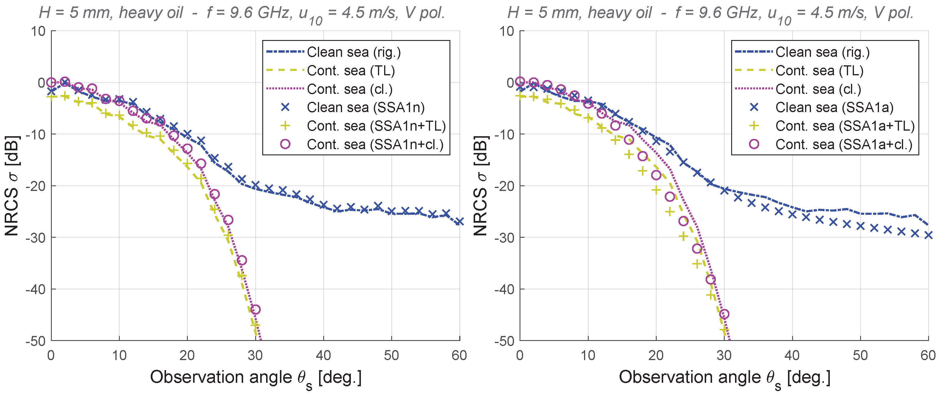
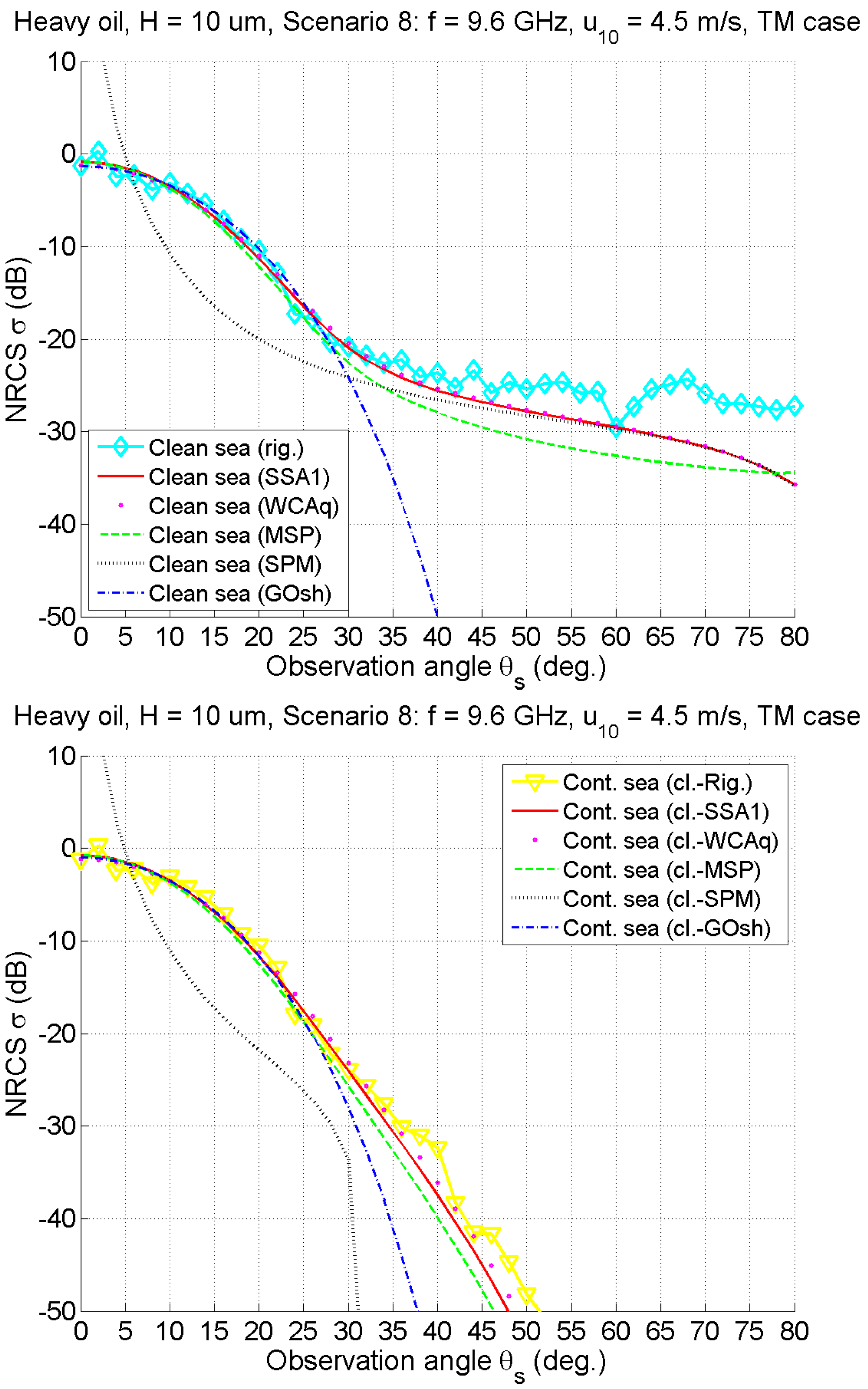
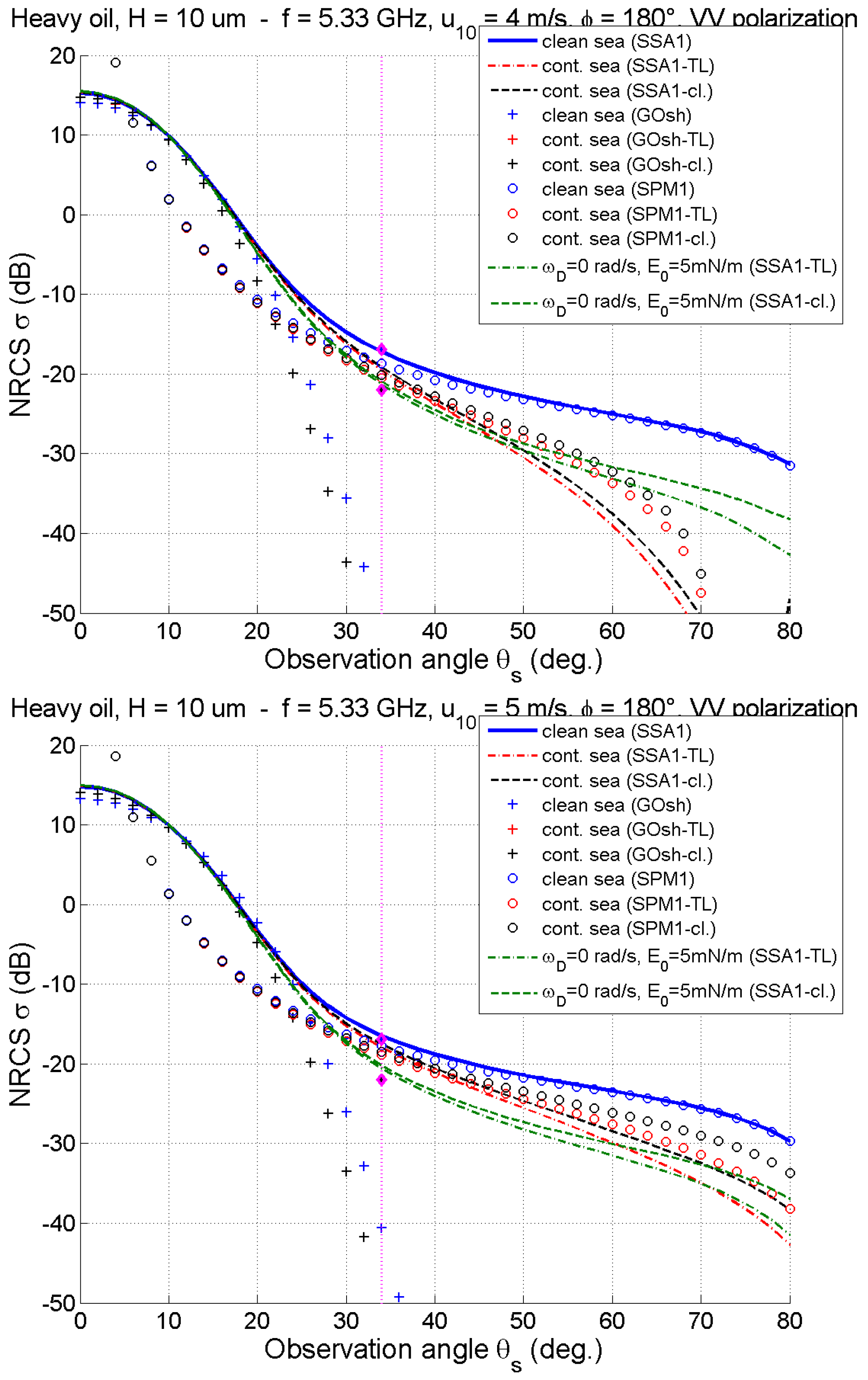
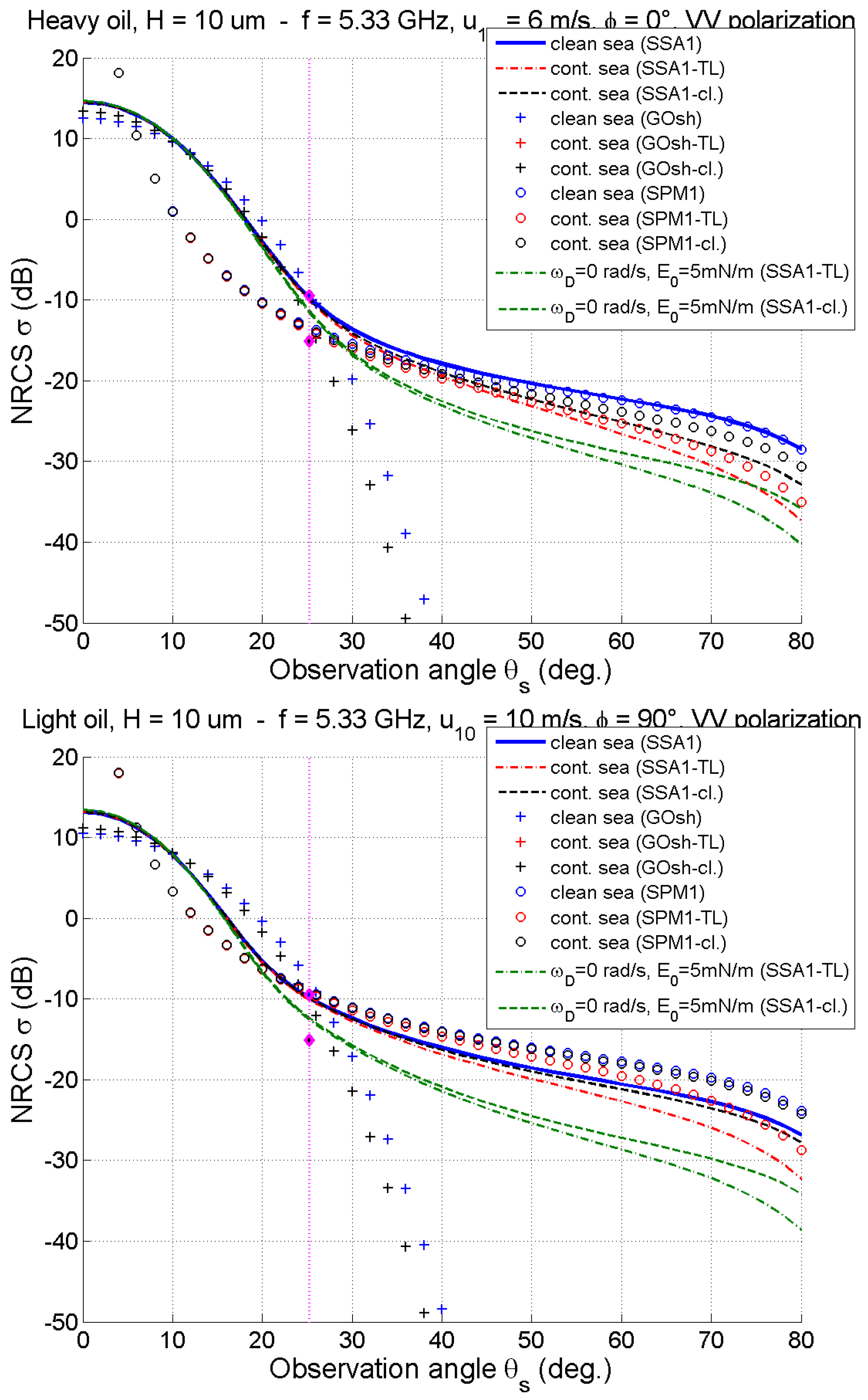
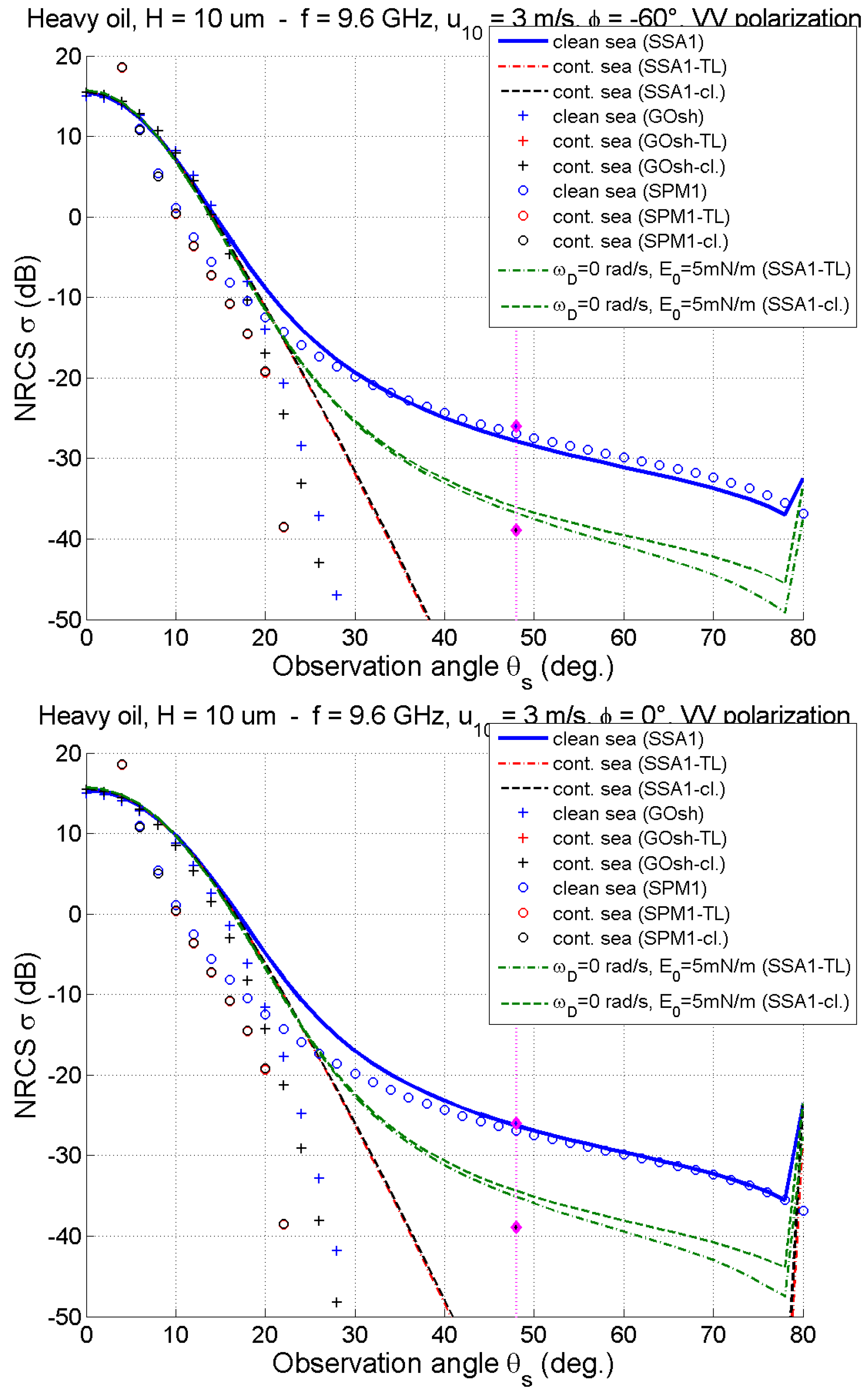
2D Validation of Common Asymptotic Models for Clean and Contaminated Seas

In order to validate asymptotic electromagnetic models commonly used for sea-like surfaces (SSA1, WCA, LCA, … [19]) in 2D, we will focus on a realistic configuration based on measurements for which the geophysical parameters (incidence angle, frequency, polarization; wind speed and direction) and oil slick parameters (age, viscosity, composition, volume) are known. This data has been provided by CLS company. Here, as we deal with 2D problems, we took a set of data for which the sensor is in the (up- or down-) wind direction. Then, we took here the second set of data of the Norway measurement campaign (NOFO oil-on-water exercise [28]—near Bergen), dated 9 June 2011 (21 h 29${}^{\prime }$ UTC). Indeed, the azimuth angle with respect to the wind direction was estimated to be ${180}^{°}$ for this set. The other estimated parameters are: wind speed $u_{10}=4.5$ m/s, incidence angle ${\theta }_i={34}^{°}$. The radar frequency $f=9.65$ GHz (TerraSAR-X sensor), with $\mathrm{VV}$ polarization. About the oil slick parameters, the viscosity can be estimated from the knowledge of the viscosity before damping at sea and of the temporal evolution of the viscosity after damping. For the last aspect, we took information from the RAPSODI project [33] (Appendix 1). The measurement was led 12 h after the oil damping. Then, knowing that damped oil was light oil, the oil at sea at the moment of the measurement was heavier, on the order of 50 cm${}^2$/s. Moreover, in order to model the oil emulsification, we take the same value as previously, that is ${ϵ}_{r2}^{eq}=17+4i$. Last, knowing the volume of damped oil and the oil slick detected surface (by taking into account mostly the oil evaporation), we can estimate the mean thickness of the oil as on the order of 10 $\mathsf{\mu }$m (keeping in mind that the thickness is usually not perfectly homogeneous). Thus, all these parameters are retained for the 2D simulations to be shown hereafter, with 2 main differences: we will plot all the incidence angle range from 0 to ${60}^{°}$, and for the rigorous calculation of the contaminated sea, we must have a thick enough oil film (for the numerical method to converge) and take $H=5$ mm. The measurement results showed that around detected oil pollution, the average NRCS of the clean sea is around $-17$ dB and the one in the contaminated sea is around $-22$ dB, which makes an average contrast of around 5 dB.

Figure 9 presents associated numerical results, where the SSA1 [19,34] is applied comparatively to rigorous approaches, in order to evaluate the impact of applying an asymptotic method on the degradation of the NRCS. For clean sea, SSA1 is compared with the rigorous numerical method; for contaminated sea, SSA1 is applied to both TL and classical approaches, and compared to these two approaches without applying any asymptotic method such as SSA, WCA, LCA. In the left-hand side figure, the SSA1 calculated numerically (“SSA1n”) is applied, whereas in the right-hand side one, it is the SSA1 calculated analytically (“SSA1a”). For comparing numerical computations with analytic computations, a Monte-Carlo process has been used, by generating several interfaces and averaging the results.

Plotting the numerical SSA1 makes it possible to check the validity of the SSA1 on the same parameters as for the rigorous computation. Let us then first focus on the numerical SSA1 in the left-hand side figure. A general very good agreement of the numerical SSA1 with the rigorous computation is found, in each of the three plotted cases (clean sea, contaminated sea with either TL or classical approach). Then, applying the numerical SSA1 on the TL and classical approaches does not significantly degrade the approximation. The same way was used for the Weighted Curvature Approximation (WCA) [19] and gave very similar (and even slightly better) results. Using the same way, the Kirchhoff-tangent plane approximation (KA—calculated either without further approximation or with the high-frequency approximation, KA-HF, also called method of stationary phase) gives very satisfactory results up to around ${35}^{°}$. Beyond this incidence angle, it underestimates the NRCS by about 2 dB (and more for increasing angles). Thus, the SSA1 appears to be a good candidate for its use in its analytic form, in order to predict the NRCS of both clean and contaminated seas for moderate incidence angles, and with a view to extension to 3D configuration.

The results associated with the analytic SSA1 are shown in the right-hand side of Figure 9. First, for the clean sea, a good agreement of analytical SSA1 with the rigorous numerical computation can be seen, but only up to around ${40}^{°}$. Indeed, beyond this limit, the numerical computation is higher than the “SSA1a” of about 3–4 dB, up to ${60}^{°}$. Our experience on the validity domain of SSA1 leads us to say that it should correctly predict the NRCS for such a configuration, at least up to ${60}^{°}$. Then, we may attribute this difference mainly to the numerical computation which overestimates the NRCS for moderate incidence angles. We chose to take surfaces of same length for both clean and contaminated seas, in order to compare the same things. For this case, generated surfaces were of length $L=34.0$ m, with spatial sampling step $\Delta x=\lambda /8$, owing to limited computing resources. Yet, theoretically, in order to have an accurate representation of the physical phenomenon of scattering from an infinite sea-like surface, we know that we must generate surfaces of minimum length $L_{min}$ given by the relation $2\pi /L_{min}=k_{min}=0.3k_p$, where $k_p$ is the peak wavenumber such that $k_p=\Omega g^2/u_{10}$ (with $g=9.81$ m${}^2$/s the acceleration of gravity and $\Omega$ the inverse of the wave age, that we take as $0.84$ for fully-developed seas). Thus, for a wind speed $u_{10}=4.5$ m/s, the minimum surface length is about $L_{min}\simeq 61$ m, which is nearly twice generated surfaces. This qualitative calculus confirms the limitations of presented numerical results to quantitatively predict the NRCS with accuracy for this configuration, due to computing resources constraints. This also highlights the interest of using an (appropriate) analytical method such as SSA1 to deal with such problems.

Hereafter, we take the same scenario, but with a more realistic oil film thickness for illegal oil spills discharges applications: we take the previously estimated value of $H=10$ $\mathsf{\mu }$m. As a consequence, there is no rigorous numerical calculation for the contaminated sea, as the rigorous method cannot deal with such thin films at these frequencies. The objective here is then to see if we retrieve, from 2D simulations, a contrast similar to the one obtained from 3D measurements. Figure 10 compares the results of the clean sea (top) and of the classical approach of the contaminated sea (bottom) computed rigorously and with different analytical asymptotic models: the SSA1, but also the WCA (with quadratic approximation, WCAq), the method of stationary phase (MSP, approximation based on the Kirchhoff-tangent plane approximation), the small perturbation method (SPM), and the geometric optics approximation by taking the shadowing effect into account (GOsh). Similar comparisons on the TL approach for the contaminated sea were also led, leading to very similar results; that is why they are not plotted here. We recover common results: for incidence angles lower than around 20–30${}^{°}$, the scattering process is mainly governed by a GO-like behavior, which characterizes the contribution of the gravity waves. Note that this limit is rather 20–25${}^{°}$ for the clean sea and rather 25–30${}^{°}$ for the contaminated sea, which is consistent with the damping of the capillary waves by the oil film.

Conversely, for the clean sea, it can be seen that the SSA1 tends to the SPM from 35–40${}^{°}$. By contrast, for the contaminated sea, it is interesting to see that the SPM vanishes from ${30}^{°}$, which can easily be explained. Indeed, as explained in previous work [16], for 2D problems the SPM is proportional to the surface curvature spectrum $k_B^{3}S\left(k_B\right)$, evaluated at the Bragg wavenumber $k_B=2k_{0}sin{\theta }_i$, with $k_0$ the electromagnetic wavenumber. Thus, if we calculate $k_B$ and report it on the $k^{3}S\left(k\right)$ spectrum, we can see that, for this configuration, it is null for the contaminated sea from ${\theta }_i={30}^{°}$. By contrast, using the SSA1 makes it possible to correctly evaluate the NRCS beyond ${30}^{°}$. Then, conversely to the angular validity domain of GO, the one of SPM strongly decreases owing to the oil film (and may not be valid at all like here), because the gravity waves are strongly damped for heavy oil. In this specific case, the SPM is never the only contributor to the total NRCS, or in other words the so-called “capillary waves” can never describe the scattering process alone, at least with this model of surface spectrum damping and this type of oil, for this typical configuration. However, it is important to note that they are not negligible, or at least the gravity-capillary waves: they contribute to the scattering process from around ${30}^{°}$ here, as the GOsh model is not enough alone to correctly predict the NRCS.

Besides, about the results of the other asymptotic modes, as expected the MSP has an angular validity domain larger than that of the GOsh, which can easily be explained by the fact that the GOsh is based on the MSP, but with additional hypotheses, leading to a more restricted validity domain. As expected, the MSP is though less accurate than the SSA1. Last, the WCAq gives results very similar to that of the SSA1, and seemingly slightly better. Still, this observation depends on studied configurations, and the extension of the WCA model to 3D problems is more complex to implement. Thus, the SSA1 model has an excellent compromise between accuracy, complexity of implementation and computing time. That is why it is elected for its extension to 3D problems, for dealing with both clean and contaminated seas.

Thus, for the contaminated sea, as thoroughly studied in previous work for thick oil films of several millimeters [16], in general we can say that the TL approach gives the best performances for low incidences angles, around ${\theta }_i\lesssim {25}^{°}$, compared to the classical approach which is more adapted for moderate incidence angles ${\theta }_i\gtrsim {25}^{°}$. However, in the context of detection of illegal oil spill discharges, the oil film thicknesses are mostly of the order of a few tens of micrometers. Thus, in this case the classical approach is enough for dealing with contaminated seas, whatever the incidence angle.

5. Results for a 3D Problem: Validation by Measurements

Thus, for low-to-moderate incidence angles, we compare the results of the analytical SSA1, for which the contaminated sea is modeled by using the classical approach, with satellite measurement results provided by CLS. The comparisons are led on two different experiments: the first one is CSK experiment in March 2011 (X band), and the second one was led in June 2011 in Finland, off Bergen (C and X bands) and corresponds to NOFO oil-on-water exercise [28].

5.1. Comparisons with CSK Experiments (March 2011)

Let us start with the CSK experiment led in March 2011, for which the radar works at $9.61$ GHz in $\mathrm{VV}$ polarisation. 4 scenarios were recorded: see Figure 11 for the representation of the NRCS of the SAR images used for studying these scenarios. The first scenario is dated 10 March 2011, 17 h 51${}^{\prime }$41${}^{″}$. It is taken in the Mediterranean Sea, in the Gulf of Lion, south of Marseille, France (the oil spill is located about ${42}^{°}{9}^{\prime }$ N, $5^{°}{8}^{\prime }$ E). Estimated measurement conditions are as follows: the average wind speed $u_{10}=6.3$ m/s and direction relatively to the sensor $\varphi -{\varphi }_0=+{60}^{°}$, the mean incidence angle ${\theta }_i=27.6^{°}$. Thus, average measured NRCS are $-11.3$ dB for the clean sea and $-13.9$ dB for the contaminated sea, which makes a contrast of around $2.6$ dB.

For the comparisons between these measurements and 3D simulations, the estimated average wind speed was $6.3$ m/s; then, we tested the results for 6 m/s (top figure) and 7 m/s (bottom figure) (available MLB data was only for integer values of $u_{10}$ and we chose not to interpolate these data within). Moreover, about the hydrocarbon pollution, we considered a heavy oil (kinematic viscosity ${\nu }_{oil}=50$ cm${}^2$/s) of mean thickness $H=10$ $\mathsf{\mu }$m. On Figure 12, the 3D analytical simulations present the results of the SSA1, but also of the geometric optics approximation with shadowing effect (GOsh) and of the first-order small perturbation method (SPM1). For both clean and contaminated seas, we retrieve common behaviors: for low incidence angles, the SSA1 tends to the GOsh, whereas for rather high incidence angles, it tends to SPM1. However, for the contaminated sea, this behavior is not fully retrieved. This is due to the fact that the contaminated sea spectrum is strongly damped in the capillary wave regime. Thus, for $u_{10}=6$ m/s, the SPM model becomes 0 from ${60}^{°}$, because the contaminated spectrum evaluated at the Bragg wavenumber $k_B$ vanishes (see top figure of Figure 13). By contrast, as the MLB model (contrary to the Marangoni effect) depends on the wind speed, for $u_{10}=7$ m/s, this damping behavior of SPM does not appear, because this time at $k_B$ the contaminated spectrum decreases but does not vanish for all ${\theta }_i<{80}^{°}$ (see bottom figure of Figure 13).

Besides, by comparison with measurement results at ${\theta }_i=27.6^{°}$ (see purple dotted vertical line and diamonds), a very good agreement of the SSA1 results with the measurements is observed for $u_{10}=7$ m/s, for both clean and contaminated seas. Note that at this incidence, the results from both the TL and classical approaches give very similar results; they differ sensitively only from around ${60}^{°}$, where the classical approach is assumed to be more reliable. In addition, note that, like in 2D, the analytical SSA1 does not predict significant differences in the polarization ratio between clean and contaminated seas at this incidence (not plotted here).

For scenario 2, it is dated 15 March 2011, 18 h 32${}^{\prime }$. It is taken in the West of the Iroise Sea, West of Brest, Brittany, France (the oil spill is located about ${48}^{°}{9}^{\prime }$ N, $6^{°}{22}^{\prime }$ W). Estimated environmental parameters are as follows: $u_{10}=10.4$ m/s and $\varphi -{\varphi }_0=-{149}^{°}$; the mean incidence angle being ${\theta }_i=41.0^{°}$. However, the simulation results for these parameters significantly overestimate the measurement results, even for the clean sea. It is all the more unexpected as these asymptotic models tend to slightly underestimate the NRCS from wind speeds about $u_{10}\gtrsim$ 8–10 m/s. Then, it seems like the wind speed and/or direction during the measurement significantly differ(s) (i.e., lower wind speed and/or wind direction closer to cross-wind direction). As a result, for the simulations, we modified these two parameters separately and represented each configuration which best fits the clean sea result, keeping in mind that the main objective is to check if the NRCS contrast is well estimated by our modeling (again, available MLB data was only for integer values of $u_{10}$ and we chose not to interpolate these data within). Then, Figure 14 compares the measurement results with 2 different configurations: $u_{10}=7$ m/s and $\varphi -{\varphi }_0=-{149}^{°}$ on the top figure, and $u_{10}=10$ m/s and $\varphi -{\varphi }_0=-{90}^{°}$ on the bottom figure. A good agreement is also found in this scenario between the measurement and the simulations, for both clean and contaminated seas. On the bottom figure, the contrast is less well predicted by the simulation; but here we took light oil instead of heavy oil which involves a lower contrast, as we did not have the corresponding data. Similar conclusions as in Figure 12 can be led.

Let us continue our analysis with scenario 4. We keep scenario 3 for the end, as it is a specific case of low wind, for which the conclusions differ slightly from other scenarios. Then, Figure 15 presents the simulation results of scenario 4, which has the following characteristics: it is dated 10 March 2011, 17 h 51${}^{\prime }$. It is taken in the Mediterranean Sea, in the Gulf of Lion-South of Marseille, France, so it corresponds to the same SAR image, but with another spill (this oil spill is located about ${41}^{°}{55}^{\prime }$ N, $4^{°}{30}^{\prime }$ E). Estimated measurement conditions are as follows: $u_{10}=6.4$ m/s, $\varphi -{\varphi }_0=+{60}^{°}$, and ${\theta }_i=31.1^{°}$. After testing the simulations for both $u_{10}=6$ m/s and $u_{10}=7$ m/s, it seems like the actual wind speed is rather $u_{10}=6$ m/s (see Figure 15). Once more, the simulation results are in very good agreement with the measurements, which suggests that the MLB hydrodynamic model may be valid.

Last, scenario 3 has the following characteristics: it is dated 11 February 2011, 05 h 41${}^{\prime }$. It is taken in the Mediterranean Sea, in the Gulf of Lion—South of Marseille, France (the oil spill is located about ${43}^{°}{0}^{\prime }$ N, $5^{°}{0}^{\prime }$ E). Estimated measurement conditions are as follows: $u_{10}=2.5$ m/s, $\varphi -{\varphi }_0=+{160}^{°}$, ${\theta }_i=50.1^{°}$. It differs from the other three mainly by the wind speed, which is significantly lower than previously: indeed, $u_{10}=2.5$ m/s is lower than 5 m/s, which is considered as low wind. Moreover, the mean incidence angle is also higher (${\theta }_i=50.1^{°}$), which implies that the NRCS levels are significantly lower than previously. Thus, for the contaminated sea, the levels are weak and vary sensitively, between around $-30$ dB and $-34$ dB, which corresponds to the noise floor of the measurement system.

Besides, after tests on the wind speed by comparing the measured and simulated clean sea levels, it seems that the wind speed at the time of measurement is rather comprised between 3 and 4 m/s; then, these two values are retained for the simulation comparisons in Figure 16 (3 m/s on the top figure and 4 m/s on the bottom figure). The wind direction has been kept in both cases, as it is close to the configuration for which the NRCS is maximum ($0^{°}$, ${180}^{°}$ or ${360}^{°}$).

The comparison between the measurement and the simulation results show that, for the contaminated sea, the measurement predicts a level of NRCS far much higher than that of the simulation based on the MLB, whatever the approach (TL or classical). However, measured level corresponds to the noise floor of the sensor: there is finally no contradiction between these 2 results, and the MLB is not unvalidated.

Then, these results highlight the relevance of the MLB model and its very good agreement with the measurements in X band and for moderate wind speeds. For low wind speeds (typically, less than 5 m/s), there is no observable disagreement, owing to the noise floor of the sensor: the measurement configuration does not allow us to conclude on the accuracy of the MLB model for low winds and moderate-to-high incidence angles.

The following section compares the simulations with a measurement campaign led in June 2011 off Bergen (Finland), during the oil-on-water (OOW) NOFO exercise [28].

5.2. Comparisons with OOW NOFO Experiment (off Bergen, Finland, June 2011)

Three scenarios were recorded: see Figure 17 for the representation of the NRCS of the SAR images used for studying these scenarios. This experiment has the advantage of showing results for two different frequency bands: C ($f=5.33$ GHz) and X ($f=9.60$ GHz) bands. However, the measurements in X band correspond to low winds; thus, we may be faced to the noise floor of the sensor. Besides, we must keep in mind that for the measurement campaign, the marine oil slick was first contained by an oil boom, which may sensitively modify its hydrodynamic behavior (damping of capillary waves, spreading, etc.), and thus the electromagnetic response.

Let us begin with the last comparisons made in 2D (see Figure 10—$u_{10}=4.5$ m/s, ${\nu }_{oil}=50$ cm${}^2$/s, $H=10$ $\mathsf{\mu }$m, TM pol.), but with frequency $f=9.6$ GHz instead of $f=5.33$ GHz. It concerned the satellite measurements provided by CLS during the measurement campaign off Bergen (Finland) in early June 2011, during the OOW NOFO exercise. More precisely, it is located in the Frigg gas field, which is situated 230 kilometres northwest of Stavanger ($59°59\prime$N, $2^{°}27\prime$ E). More details about his experiment may be found in references [28,35]. This measurement, called scenario 2 here, was made on 9th June at 21 h 28${}^{\prime }$ UTC, and the oil spill is located about ${60}^{°}5\prime$ N, $2^{°}35\prime$ E. The measurement conditions were estimated as follows: $u_{10}=4.5$ m/s, $\varphi -{\varphi }_0=+{180}^{°}$, ${\theta }_i=34.0^{°}$. Moreover, the average oil film thickness was estimated to be around 10 $\mathsf{\mu }$m, with heavy oil of kinematic viscosity of 50 cm${}^2$/s. The equivalent relative permittivity of emulsified oil in seawater does not matter in this case, as in what follows, we will mainly focus on the classical approach. We took the same value as previously, that is, ${ϵ}_{r2}=17+4i$. The measurement results gave a mean NRCS of $-17$ dB for the clean sea and $-22$ dB for the contaminated sea, which makes a contrast of around 5 dB.

Figure 18 presents the numerical simulation results for the above quoted parameters, with the difference that considered wind speed is 4 m/s on the top figure and 5 m/s on the bottom figure. Indeed, for the contaminated sea, it is recalled that we have the spectrum data (MLB) only for integer values of $u_{10}$. As a general remark, the same behaviors as in 2D are recovered, which were though led in X band ($f=9.6$ GHz). Note that the 3D results do not have the same variations as in 2D: it is not enough to make 2D simulations to predict the 3D levels. Nevertheless, from the analytical formulations of the SSA1 in 2D and 3D, the connection can be found rather easily. The main problem for the 2D model is then the taking into account of the wind direction. For the clean sea, the GO and SPM limits of SSA1 are recovered for low and high incidence angles, respectively. For the contaminated sea, the GO limit is recovered. Still, owing to the capillary wave damping by the oil film, the SPM limit is not reached. A simple reason is that here the SPM vanishes from ${45}^{°}$.

The comparison of the levels of NRCS at ${34}^{°}$ with the measurement results appear in magenta with diamonds. They are rather good at 4 m/s for the MLB model and are most probably closer to reality, as at 5 m/s, the SSA1 results of the clean sea slightly overestimate the measured NRCS. Here, the MLB overestimates the NRCS of the contaminated sea.

Figure 19 presents the numerical results of scenario 3 of the NOFO campaign. This measurement was made on 12th June at 21 h 18${}^{\prime }$ UTC, and the oil spill is located about ${60}^{°}7\prime$ N, $2^{°}25\prime$ E. Estimated measurement conditions are as follows: $u_{10}=5.8$ m/s, $\varphi -{\varphi }_0=+{90}^{°}$; the mean incidence angle being ${\theta }_i=25.2^{°}$. However, the results for $u_{10}=5.8$ m/s and $\varphi -{\varphi }_0=+{90}^{°}$ significantly underestimate the NRCS, even for the clean sea. Thus, the wind speed is underestimated and/or the wind direction is closer to $0^{°}$ or ${180}^{°}$ (upwind or downwind direction). We tested the distinct influence of the two variations: 6 m/s and $0^{°}$ on the top figure, and 10 m/s and $+{90}^{°}$ on the bottom figure. Note that a priori, the first configuration seems the most probable, because for the second configuration, the difference with the estimation in the wind speed is very high.

Even if the results for the two chosen configurations vary in general, around the measurement incidence ${\theta }_i=25.2^{°}$, the results are similar. They show that, contrary to the measurements, the MLB model predicts a negligible contrast. However, we are not in the case of low wind any more. Then, this may highlight the limits of the MLB model in the C band. This could be confirmed by the measurements on illegal oil spill discharges by emptying of fuel tanks, such as for CSK measurements, but in the C band. Indeed, another possible explanation of this difference is the conditions of the experiment: the marine oil pollution was contained in an oil boom, which may significantly modify its hydrodynamic behavior: its spreading over time, as well as its damping characteristics, or its thickness H. Then, we led numerical tests for different values of H, by assuming the same viscosity (heavy oil). The best agreement was found for $H=1000$ $\mathsf{\mu }$m. This is possible, as we do not know the origin of this pollution. Indeed, this scenario corresponds to a measurement dated 12th June, that is, 3 days after the last damping. Thus, this slick may correspond either to a slick of the measurement campaign or a slick of unknown origin. In the first hypothesis, owing to elapsed time (at least 3 days), the slick is much more viscous than previously, which we did not consider in our data based on the MLB. Thus, modeling a greater viscosity artificially by a greater thickness makes sense, even if it is only qualitative and if the quantitative results would differ. Yet, emulsification over time tends to increase the film thickness, making this analysis not stupid. In the second hypothesis, it is impossible to conclude without the knowledge of this slick. Thus, this result is not very much relevant.

Figure 20 presents the results of scenario 1 (X band, $f=9.6$ GHz). This measurement was made on 8th June at 17 h 58${}^{\prime }$ UTC, and the oil spill is located about ${60}^{°}3\prime$ N, $2^{°}32\prime$ E. Estimated measurement conditions are as follows: $u_{10}=2.6$ m/s, $\varphi -{\varphi }_0=-{60}^{°}$, ${\theta }_i=48.0^{°}$. For the simulations, $u_{10}=3$ m/s was chosen because it gave a better fit with the clean sea measurement; 2 configurations are then represented: $\varphi -{\varphi }_0=-{60}^{°}$ on the top figure and $\varphi -{\varphi }_0=0^{°}$ on the bottom figure. The results show that the MLB model predicts a much higher contrast than the measured one. Still, the NRCS level of the contaminated sea corresponds to the noise floor of the sensor for this configuration. Thus, the real contrast is at least as much important: this does not contradict with the MLB model.

As a conclusion, the comparison of the MLB model (combined with the classical approach and the SSA1 method) with the measurement results generally give good or even very good agreement, and in particular in X band for moderate winds. For low winds, the noise floor of the sensor does not allow us to evaluate the accuracy of the MLB model, but at least we can say that these specific results do not contradict the MLB predictions. In the C band, the results are more limited; they would deserve to be completed before being able to lead conclusions.

As mentioned in the introduction (4th paragraph), the existing literature used to applying only the SPM1 (single Bragg scattering mechanism) [22,23,24]. Nevertheless, as pointed out in this work (see in particular Figure 10) as well as in [4,22], the single Bragg scattering mechanism is not always enough to describe the scattering mechanisms. Then, recent works considered unified EM methods: most of the time, it is the tilted Bragg or two-scale model (TSM) that is applied [4,12,22,25,26]. This choice is probably due to its relative simplicity of implementation. It may also be noted that it generally slightly better predicts the polarization behaviour, as compared to SSA1 [36]. Nevertheless, like for clean sea surfaces, the choice of the cutoff wavenumber for distinguishing the small-scale Bragg components from the large scale GO ones must be analyzed for oil slicks, and it has an impact on the NRCS at the transition between the two regimes (about 20–30${}^{°}$), where the TSM has poorer performances. Besides, the damping model that is considered is often more simple and less adapted. In particular, the Marangoni damping model [15] (see for instance [4,25]) cannot handle the oil film thickness. It is in consequence applicable mainly for very thin oil film (theoretically, mono-molecular films). By comparison, recent works [24,37] which applied the Jenkins and Jacobs damping model [38] are more adapted, the necessary condition being to be able, like for the MLB model, to determine its physical parameters appropriately. Lastly, one great advantage of the present work has been to check the validity of all applied approximations: first, for 2D problems by comparison with a rigorous numerical method, and then, for 3D problems by comparison with measurements. Not only the asymptotic models have been tested, but also (which is to our knowledge a noticeable originality) the TL and classical approaches for reducing the double layer problem to a single layer one.

Thus, the MLB model, combined with the classical approach and the SSA1 method, seems to be a good tool for describing the radar NRCS of seas contaminated with marine oil, at least in X band. Note that, unfortunately, only the $\mathrm{VV}$ polarization was measured here. It would be interesting to lead the same analysis in $HH$ polarization. This would make it possible, for instance, to study the copolarization ratio behavior in 3D (following the work led in 2D [16]), comparatively to that of the clean sea, and more generally, to further check if some other observed polarimetric features [35] are retrieved by proposed modeling. Note that, for being able to predict the polarization behaviour with good accuracy, it may be necessary to rather apply the second-order SSA. It is particularly true for higher wind speeds (typically, for $u_{10}>$ 8–10 m/s), where it is well-known (for clean sea surfaces at least) that so-called first-order unified models (like the classical TSM or the SSA1) are not enough anymore to correctly predict the scattering mechanisms. In this case, it is then also necessary to take into account the non-linearities of the surfaces. A first step for doing so, before dealing with the much more complex case of breaking waves, is to apply a so-called choppy wave model [39], for instance.

6. Conclusions

This paper presented refined asymptotic approaches that make it possible to rapidly and precisely calculate the electromagnetic wave scattering from both clean seas and seas contaminated by marine oil surfactants, with several validations. As input parameters, the hydrodynamic modeling is realized by applying the well-known Elfouhaily et al. [14] spectrum for clean seas. The surface wave damping in the presence of oil films is handled by applying the local equilibrium model (MLB) [17], a refined model that (among other parameters) takes the oil film thickness influence into account.

Then, once the realistic sea-like surfaces are defined (and generated when a numerical EM method is elected), a strategy has been proposed for reducing the complex double layer problem (air/oil and oil/sea) to a single interface one, by testing 2 simplifying approaches: the so-called “Thin-Layer” (TL) and classical approaches. These two approaches have been tested directly on the rigorous numerical method (based on the MoM) and confirmed previous studies [16]: the TL approach is valid for small incidence angles (${\theta }_i\lesssim {30}^{°}$), which is logical as it is based on a Kirchhoff-tangent plane assumption of locally flat interfaces. Then, this approach is all the more valid as the capillary waves are damped, corresponding to films of larger thickness or viscosity, in particular. By contrast, for very thick oil films of a few millimeters [16], the classical approach is valid for moderate angles, but the accuracy degrades for smaller angles, in particular for the scenario of emulsified oil tested here. Nevertheless, for thinner oil films ($H=10\mathsf{\mu }$m tested here), more representative of illegal oil spill discharges, the classical approach tends to the TL approach for small angles, making it valid and accurate even for small angles. Thus, the classical approach may be used for illegal oil spill discharges for all moderate incidence angles.

Second, in order to calculate the electromagnetic scattering even faster, several asymptotic electromagnetic models (combined with either the TL or the classical approach) were tested. Among others, the first-order small-slope approximation (SSA1) model [34] was implemented and thoroughly analyzed. It presents the advantage of having a very good compromise between rapidity and accuracy of the calculation: it is well-known to be valid for a wide range of incidence angles (up to about ${60}^{°}$), and for low-to-moderate wind speeds. Its extension to the case of contaminated seas, by using the TL and classical approaches, was validated by comparison with the MoM. Comparisons with other asymptotic models (results were shown only for their analytic version) made it possible to study the validity domain of these models when applied to contaminated seas. The main features are: the scattering process is mainly governed by a GO-like behavior for incidence angles less than about 25–30${}^{°}$, to be compared with 20–25${}^{°}$ for clean seas. This is in agreement with the fact that the oil film strongly damps the capillary waves. This feature has an impact on the validity domain of the SPM (Bragg scattering mechanism), which mainly governs the scattering process for higher incidence angles than for clean seas, which is usually about 35–40${}^{°}$. Depending on the scene configuration and on the oil film characteristics, this validity domain may either remain unchanged or on the contrary not be valid at all any more, as illustrated in Figure 10 and confirmed further in the paper.

Last, developed methods have been extended to realistic 3D problems, where comparisons with satellite measurements were led. The two sets of experiments (CSK experiments and OOW NOFO experiment) made it possible to test developed methods for different configurations: in particular, different wind speeds and directions, incidence angles, oil film viscosities, as well as radar frequencies. The results highlighted the relevance of the MLB hydrodynamic model to quantify the NRCS of seas contaminated by marine oil surfactants. The agreements of the SSA1 model combined with the classical approach are indeed very good in X band. The main limitations are the fact that only the VV polarization was measured here, and that the frequency dependence could not reliably be analyzed. In addition, the SSA1 model is limited in terms of polarization dependence and is valid only for low-to-moderate winds. Future work may then be devoted to study the influence of the polarization, by applying for example the second-order SSA, which would extend the validity of the modeling to higher wind speeds.

References

- Solberg, A.H.S.; Brekke, C.; Husoy, P.O. Oil Spill Detection in Radarsat and Envisat SAR Images. IEEE Trans. Geosci. Remote Sens. 2007, 45, 746–755. [Google Scholar] [CrossRef]
- Derrode, S.; Mercier, G. Unsupervised multiscale oil slick segmentation from SAR images using a vector HMC model. Pattern Recognit. 2007, 40, 1135–1147. [Google Scholar] [CrossRef]
- Nunziata, F.; Gambardella, A.; Migliaccio, M. On the Mueller Scattering Matrix for SAR Sea Oil Slick Observation. IEEE Geosci. Remote Sens. Lett. 2008, 5, 691–695. [Google Scholar] [CrossRef]
- Minchew, B.; Jones, C.E.; Holt, B. Polarimetric Analysis of Backscatter From the Deepwater Horizon Oil Spill Using L-Band Synthetic Aperture Radar. IEEE Trans. Geosci. Remote Sens. 2012, 50, 3812–3830. [Google Scholar] [CrossRef]
- Zhang, Y.; Li, Y.; Lin, H. Oil-Spill Pollution Remote Sensing by Synthetic Aperture Radar. In Advanced Geoscience Remote Sensing; Marghany, M., Ed.; IntechOpen: Rijeka, Croatia, 2014; Chapter 2. [Google Scholar] [CrossRef]
- Skrunes, S.; Brekke, C.; Eltoft, T.; Kudryavtsev, V. Comparing Near-Coincident C- and X-Band SAR Acquisitions of Marine Oil Spills. IEEE Trans. Geosci. Remote Sens. 2015, 53, 1958–1975. [Google Scholar] [CrossRef]
- Fingas, M.; Fieldhouse, B. Formation of water-in-oil emulsions and application to oil spill modelling. J. Hazard. Mater. 2004, 107, 37–50. [Google Scholar] [CrossRef]
- Migliaccio, M.; Tranfaglia, M.; Ermakov, S. A physical approach for the observation of oil spills in SAR images. IEEE J. Ocean. Eng. 2005, 30, 28–39. [Google Scholar] [CrossRef]
- Fuks, I.; Zavorotny, V. Polarization dependence of radar contrast for sea surface oil slicks. In Proceedings of the IEEE Radar Conference, Waltham, MA, USA, 17–20 April 2007. [Google Scholar]
- Wu, Z.S.; Zhang, J.P.; Guo, L.X.; Zhou, P. An improved two-scale model with volume scattering for the dynamic ocean surface. Prog. Electromagn. Res. 2009, 89, 39–56. [Google Scholar] [CrossRef]
- Yang, P.; Guo, L. Polarimetric Doppler spectrum of backscattered echoes from nonlinear sea surface damped by natural slicks. J. Quant. Spectrosc. Radiat. Transf. 2016, 184, 193–204. [Google Scholar] [CrossRef]
- Panfilova, M.A.; Karaev, V.Y.; Guo, J. Oil Slick Observation at Low Incidence Angles in Ku-Band. J. Geophys. Res. Oceans 2018, 123, 1924–1936. [Google Scholar] [CrossRef]
- Pinel, N.; Déchamps, N.; Bourlier, C. Modeling of the Bistatic Electromagnetic Scattering From Sea Surfaces Covered in Oil for Microwave Applications. IEEE Trans. Geosci. Remote Sens. 2008, 46, 385–392. [Google Scholar] [CrossRef]
- Elfouhaily, T.; Chapron, B.; Katsaros, K.; Vandemark, D. A unified directional spectrum for long and short wind-driven waves. J. Geophys. Res. Oceans 1997, 102, 781–796. [Google Scholar] [CrossRef]
- Lombardini, P.; Fiscella, B.; Trivero, P.; Cappa, C.; Garrett, W. Modulation of the spectra of short gravity waves by sea surface films: Slick detection and characterization with a microwave probe. J. Atmos. Ocean. Technol. 1989, 6, 882–890. [Google Scholar] [CrossRef]
- Pinel, N.; Bourlier, C.; Sergievskaya, I. Two-dimensional radar backscattering modeling of oil slicks at sea based on the Model of Local Balance: Validation of two asymptotic techniques for thick films. IEEE Trans. Geosci. Remote Sens. 2014, 52, 2326–2338. [Google Scholar] [CrossRef]
- Ermakov, S.; Salashin, S.; Panchenko, A. Film slicks on the sea surface and some mechanisms of their formation. Dyn. Atmos. Oceans 1992, 16, 279–304. [Google Scholar] [CrossRef]
- Pinel, N.; Bourlier, C.; Sergievskaya, I. Unpolarized emissivity of thin oil films over anisotropic Gaussian seas in infrared window regions. Appl. Opt. 2010, 49, 2116–2131. [Google Scholar] [CrossRef]
- Elfouhaily, T.M.; Guérin, C.A. A critical survey of approximate scattering wave theories from random rough surfaces. Waves Random Media 2004, 14, R1–R40. [Google Scholar] [CrossRef]
- Bourlier, C.; Pinel, N. Numerical implementation of local unified models for backscattering from random rough sea surfaces. Waves Random Complex Media 2009, 19, 455–479. [Google Scholar] [CrossRef]
- Bourlier, C. Upwind—Downwind Asymmetry of the Sea Backscattering Normalized Radar Cross Section Versus the Skewness Function. IEEE Trans. Geosci. Remote Sens. 2018, 56, 17–24. [Google Scholar] [CrossRef]
- Alpers, W.; Holt, B.; Zeng, K. Oil spill detection by imaging radars: Challenges and pitfalls. Remote Sens. Environ. 2017, 201, 133–147. [Google Scholar] [CrossRef]
- Kim, D.j.; Moon, W.; Kim, Y.S. Application of TerraSAR-X Data for Emergent Oil-Spill Monitoring. IEEE Trans. Geosci. Remote Sens. 2010, 48, 852–863. [Google Scholar] [CrossRef]
- Zhang, Y.; Zhang, J.; Wang, Y.; Meng, J.; Zhang, X. The damping model for sea waves covered by oil films of a finite thickness. Acta Oceanol. Sin. 2015, 34, 71–77. [Google Scholar] [CrossRef]
- Montuori, A.; Nunziata, F.; Migliaccio, M.; Sobieski, P. X-Band Two-Scale Sea Surface Scattering Model to Predict the Contrast due to an Oil slick. IEEE J. Sel. Top. Appl. Earth Obs. Remote Sens. 2016, 9, 4970–4978. [Google Scholar] [CrossRef]
- Nunziata, F.; de Macedo, C.R.; Buono, A.; Velotto, D.; Migliaccio, M. On the analysis of a time series of X-band TerraSAR-X SAR imagery over oil seepages. Int. J. Remote Sens. 2019, 40, 3623–3646. [Google Scholar] [CrossRef]
- Jackson, C.R.; Apel, J.R. Synthetic Aperture Radar Marine User’s Manual; US Department of Commerce: Washington, DC, USA, 2004.
- Skrunes, S.; Brekke, C.; Eltoft, T. Oil spill characterization with multi-polarization C- and X-band SAR. In Proceedings of the 2012 IEEE International Geoscience and Remote Sensing Symposium, Munich, Germany, 22–27 July 2012. [Google Scholar]
- Lamkaouchi, K. Water: A Dielectric Standard. Permittivity of Water-Petrol Mixtures at Microwave Frequencies. Ph.D. Thesis, Bordeaux I University, Talance, France, 1992. (In French). [Google Scholar]
- Iodice, A. Forward-Backward method for scattering from dielectric rough surfaces. IEEE Trans. Antennas Propag. 2002, 50, 901–911. [Google Scholar] [CrossRef]
- Chou, H.T.; Johnson, J. A novel acceleration algorithm for the computation of scattering from rough surfaces with the Forward-Backward method. Radio Sci. 1998, 33, 1277–1287. [Google Scholar] [CrossRef]
- Déchamps, N.; de Beaucoudrey, N.; Bourlier, C.; Toutain, S. Fast numerical method for electromagnetic scattering by rough layered interfaces: Propagation-inside-layer expansion method. JOSA A 2006, 23, 359–369. [Google Scholar] [CrossRef]
- Cedre (Centre de Documentation, de Recherche et D’expérimentations sur les Pollutions Accidentelles des Eaux). RAPSODI (Remote Sensing Anti-Pollution System for geOgraphical Data Integration), Experimentation Report (D9); Technical Report; European Community: Maastricht, The Netherlands, 2001. [Google Scholar]
- Voronovich, A. Wave Scattering from Rough Surfaces, 2nd ed.; Springer: Berlin/Heidelberg, Germany, 1999. [Google Scholar]
- Skrunes, S.; Brekke, C.; Eltoft, T. Characterization of Marine Surface Slicks by Radarsat-2 Multipolarization Features. IEEE Trans. Geosci. Remote Sens. 2014, 52, 5302–5319. [Google Scholar] [CrossRef]
- Mouche, A.; Chapron, B.; Reul, N. A simplified asymptotic theory for ocean surface electromagnetic wave scattering. Waves Random Complex Media 2007, 17, 321–341. [Google Scholar] [CrossRef]
- Zheng, H.; Zhang, J.; Zhang, Y.; Khenchaf, A.; Wang, Y. Theoretical Study on Microwave Scattering Mechanisms of Sea Surfaces Covered with and without Oil Film for Incidence Angle Smaller Than 30°. IEEE Trans. Geosci. Remote Sens. 2021, 59, 37–46. [Google Scholar] [CrossRef]
- Jenkins, A.; Jacobs, S. Wave damping by a thin layer of viscous fluid. Phys. Fluids 1997, 9, 1256–1264. [Google Scholar] [CrossRef]
- Nouguier, F.; Guérin, C.A.; Chapron, B. Scattering From Nonlinear Gravity Waves: The “Choppy Wave” Model. IEEE Trans. Geosci. Remote Sens. 2010, 48, 4184–4192. [Google Scholar] [CrossRef]
Publisher’s Note: MDPI stays neutral with regard to jurisdictional claims in published maps and institutional affiliations. |
© 2022 by the authors. Licensee MDPI, Basel, Switzerland. This article is an open access article distributed under the terms and conditions of the Creative Commons Attribution (CC BY) license (https://creativecommons.org/licenses/by/4.0/).
Share and Cite
Pinel, N.; Bourlier, C.; Sergievskaya, I.; Longépé, N.; Hajduch, G. Asymptotic Modeling of Three-Dimensional Radar Backscattering from Oil Slicks on Sea Surfaces. Remote Sens. 2022, 14, 981. https://doi.org/10.3390/rs14040981
Pinel N, Bourlier C, Sergievskaya I, Longépé N, Hajduch G. Asymptotic Modeling of Three-Dimensional Radar Backscattering from Oil Slicks on Sea Surfaces. Remote Sensing. 2022; 14(4):981. https://doi.org/10.3390/rs14040981
Chicago/Turabian StylePinel, Nicolas, Christophe Bourlier, Irina Sergievskaya, Nicolas Longépé, and Guillaume Hajduch. 2022. "Asymptotic Modeling of Three-Dimensional Radar Backscattering from Oil Slicks on Sea Surfaces" Remote Sensing 14, no. 4: 981. https://doi.org/10.3390/rs14040981
APA StylePinel, N., Bourlier, C., Sergievskaya, I., Longépé, N., & Hajduch, G. (2022). Asymptotic Modeling of Three-Dimensional Radar Backscattering from Oil Slicks on Sea Surfaces. Remote Sensing, 14(4), 981. https://doi.org/10.3390/rs14040981