Article

Earth Observation for Phenological Metrics (EO4PM): Temporal Discriminant to Characterize Forest Ecosystems

by
Federico Filipponi
,
Daniela Smiraglia
*,† and
Emiliano Agrillo
Italian Institute for Environmental Protection and Research (ISPRA), Via Vitaliano Brancati 48, 00144 Roma, Italy
*
Author to whom correspondence should be addressed.
These authors equally contributed to this work.
Remote Sens. 2022, 14(3), 721; https://doi.org/10.3390/rs14030721
Submission received: 24 December 2021 / Revised: 28 January 2022 / Accepted: 1 February 2022 / Published: 3 February 2022

Abstract

:
The study of vegetation phenology has great relevance in many fields since the importance of knowing timing and shifts in periodic plant life cycle events to face the consequences of global changes in issues such as crop production, forest management, ecosystem disturbances, and human health. The availability of high spatial resolution and dense revisit time satellite observations, such as Sentinel-2 satellites, allows high resolution phenological metrics to be estimated, able to provide key information from time series and to discriminate vegetation typologies. This paper presents an automated and transferable procedure that combines validated methodologies based on local curve fitting and local derivatives to exploit full satellite Earth observation time series to produce information about plant phenology. Multivariate statistical analysis is performed for the purpose of demonstrating the capacity of the generated smoothed vegetation curve, temporal statistics, and phenological metrics to serve as temporal discriminants to detect forest ecosystems processes responses to environmental gradients. The results show smoothed vegetation curve and temporal statistics able to highlight seasonal gradient and leaf type characteristics to discriminate forest types, with additional information about forest and leaf productivity provided by temporal statistics analysis. Furthermore, temporal, altitudinal, and latitudinal gradients are obtained from phenological metrics analysis, which also allows to associate temporal gradient with specific phenophases that support forest types distinction. This study highlights the importance of integrated data and methodologies to support the processes of vegetation recognition and monitoring activities.

1. Introduction

Since the 1990s, under the boost of phenology networks establishment and monitoring programs initiatives, the interest in phenology has significantly increased [1,2,3,4]. Plant phenology studies the succession of plant cycle phases (e.g., leaf unfolding, flowering, blooming, leaf fall) and their development in relation to abiotic and biotic factors [5] especially with regard to meteorological components such as temperature, rainfall, humidity, radiation, exposure [6,7]. The role of phenology as a bioindicator of climate change, has been acknowledged by the World Meteorological Organization (WMO) and the Intergovernmental Panel on Climate Change (IPPC) [6,8], and the shifts in the timing of phenological stages due to climate changes have been widely recognized [9,10,11,12,13,14,15]. Phenology tracks annually recurring events in ecosystems such as plant germination, flowering, growth, and fruit maturation. Since these events are triggered predominantly by temperature, phenology has emerged as a key asset in identifying current fingerprints of climate change in nature, especially since recent warming is mirrored by significantly advancing spring events [15]. At the same time, the seasonal life cycle events throughout the year have great relevance in many fields, such as biodiversity (e.g., detection of ecosystem disturbances), cultivated species of agricultural interest (e.g., timing of management activities), forestry (e.g., monitoring forest health), and in relation to human health (e.g., providing pollen information) [2,16,17].
Nowadays, it is possible to identify time shifts and seasonal changes thank to a large amount of data set available, in some cases time series of phenological observations date back to the 19th century [18] and more [19]. This has fostered the establishment of phenological networks throughout the world, mainly based on field observations of standard growth stages of plant cycles [20], such as budburst or leaf senescence. However, ground phenology detection has some shortcomings as it is labor intensive, it involves limited geographic extents, and a limited number of species investigated [21,22,23]. On the other hand, major advances in near-surface remote sensing and satellite remote sensing have supported the developments of new methodologies of data collection and analysis from a regional to a continental scale [21,24,25]. Especially satellite remote sensing increases the range of the scale of analysis moving from plant species phenological phases to the detection of land surface phenology at the landscape scale [26,27]. It enables to investigate the spatio-temporal patterns of plant phenology and their relationship with environmental variability and climatic drivers.
The detection of phenological events by satellite remote sensing needs a dense time series of data for the purpose of being able to ascertain rapid phenological changes and to overcome the problem of cloud covered images [25,28]. To this end they made a strong contribution the Advanced Very High Resolution Radiometer (AVHHR) and Moderate Resolution Imaging Spectrometer (MODIS/Terra) sensors, providing a global coverage of very high temporal (twice daily and daily, respectively) and coarse-to-moderate spatial (1 km and 250 m, respectively) resolution observations for more than 20 years and over large geographic regions [29,30,31,32]. At present, Sentinel-2 satellites provide global acquisitions of high resolution (10–20 m) and high-revisit frequency (5 days) multispectral images enabling more detailed-scale phenological studies [33,34].
Phenology can be investigated by exploiting the optical response of vegetation through the seasonal variations of spectral and biophysical indices [35,36,37] by analyzing the vegetation index time series. Vegetation indices are the basic information for phenological researches, e.g., by analyzing the vegetation index time series to derive information [38,39,40,41,42], by assessing temporal statistics [43,44], or by estimating phenological metrics (as the onset of greenup, the length of the growing season, and the offset of the season) [45,46,47].
There are various methods to estimate the phenological metrics from vegetation index time series, namely threshold-based methods, smoothing functions, empirical equations, rate of change, change detection, phenology matching, simulation-based methods, and derivatives of vegetation greenness curves [22,25,48,49,50,51]. Data smoothing plays a key role in the estimation of phenological metrics, since it simplifies vegetation index time series curves using empirical methods, curve fitting method or data transformation methods [25]. The successful retrieval of phenological metrics depends on the availability of robust algorithms that are capable of processing vegetation time series while minimizing atmospheric noise and sensor-related errors [52]. The aim is to extract key information from the curve of phenological time series, such as the slope of the curve or the length of the plateau, and link them to a specific phenological response.
In view of climate change mitigation and adaptation measures to be adopted by different countries, high resolution phenology trends will contribute to improve a number of monitoring activities, such as ecological status, environmental conditions, climate change impacts on ecosystems, detailed land-use/land-cover mapping, the estimation of carbon storage, vegetation responses to disturbances, cropland practices, and urban ecosystem assessments [53]. Along with the availability of high resolution satellite time series and proven methodologies to extract temporal information from satellite acquisitions, comes the need for procedures to generate high resolution Earth observation derived phenological metrics that could serve a wide range of applications. In the last decade, Sentinel-2 MSI satellite sensors have contributed significantly in encouraging vegetation investigations which have led to develop methods and products [34,54,55]. In particular, the availability of high spatial resolution and dense revisit time satellite observations, opened the way to high resolution phenological metrics estimation, representing a promising tool for the study of terrestrial ecosystems and species-specific phenology. Phenological metrics are able to synthetize key information from time series and can be used to discriminate forest typologies on the basis of the observation and measuring of the ecosystem processes responses to environmental gradients.
An automated and transferable procedure that combines available validated methodologies to exploit full satellite Earth observation time series to produce rapid and updated information about plant phenology, without any a priori information and without an excessive simplification of the temporal curve, is here presented. The aims of this study are: (i) to present a procedure to estimate phenological metrics and temporal statistics from high spatial resolution satellite images, exploiting a dense and smoothed time series of the Leaf Area Index (LAI); (ii) to investigate if smoothed vegetation curve, temporal statistics, and phenological metrics may contribute as temporal discriminants to characterize forest ecosystems in Italy.

2. Materials and Methods

2.1. Study Area

Italy is situated in the Mediterranean basin and covers about 300,000 km2 (Figure 1). It is characterized by two main mountain ranges (the Alps and the Apennines), hilly zones, river valleys, and a coastline of about 7600 km. The physiography and geographical position have led to it having heterogeneous features in terms of climate (ranging from a Mediterranean climate in the south and along the coastline, to a Temperate climate in the north and in the mountains) and in terms of land use along latitudinal and elevation gradients [56,57].
Land use is mainly represented by agricultural (52%), natural (43%) and artificial (5%) areas. Most of the natural areas are forests (28%) which are diversified into multiple habitat types.

2.2. Forest Habitat Types

The European Vegetation Archive (EVA) dataset [58,59] was used in this work. The archive includes georeferenced vegetation plots with species list and cover abundance. The sub-dataset used in this study takes into account vegetation plots smaller than 200 m2 and with a geographic localization accuracy ranging from 0.1 to 30 m. Following the EUNIS (European Nature Information System) II and III level hierarchical classification nomenclature [60] 14,385 plots from the EVA dataset were selected and classified (Table 1) [61]. Figure 1 shows the spatial distribution of forest stands along the Italian peninsula at II level EUNIS classification. These forest types at EUNIS level II were used to estimate the smoothed vegetation curve and the temporal statistics, while regarding the phenological metrics estimate, only deciduous broadleaved forest types (T1) at EUNIS III level were considered from the vegetation plot records of the archive, since for the evergreen forest types is more difficult to identify the timing of the onset of greenness and senescence due to the lower temporal fluctuation of the vegetation index time series [61,62] and snow prevalence during wintertime in mountain ecosystems [55], hiding evergreen forests.

2.3. Satellite Data

Sentinel-2 (S2) satellite acquisitions acquired during the year 2019, with cloud cover lower than 90%, were gathered for the study area (around 7000 images, 61 granules, 9 Terabyte of data stored). The high spatial resolution (10 m, 20 m and 60 m), the high revisit time (5 days with two satellites), and the 13 spectral bands (from the visible to shortwave infrared) are the characteristics of the S2 Multi-Spectral Instrument (MSI) sensor. The images, distributed by Theia (MUSCATE format) as the bottom of the atmosphere (BOA) reflectance, orthorectified, terrain-flattened and atmospherically corrected with MACCS-ATCOR Joint Algorithm (MAJA) [63,64], were processed for spatial resampling of the spectral bands at 20 m and masked for invalid pixels (cloud, cloud_cirrus, cloud_shadow, topographic_shadow, snow, edge, and sun_too_low).

2.4. Satellite Data Processing

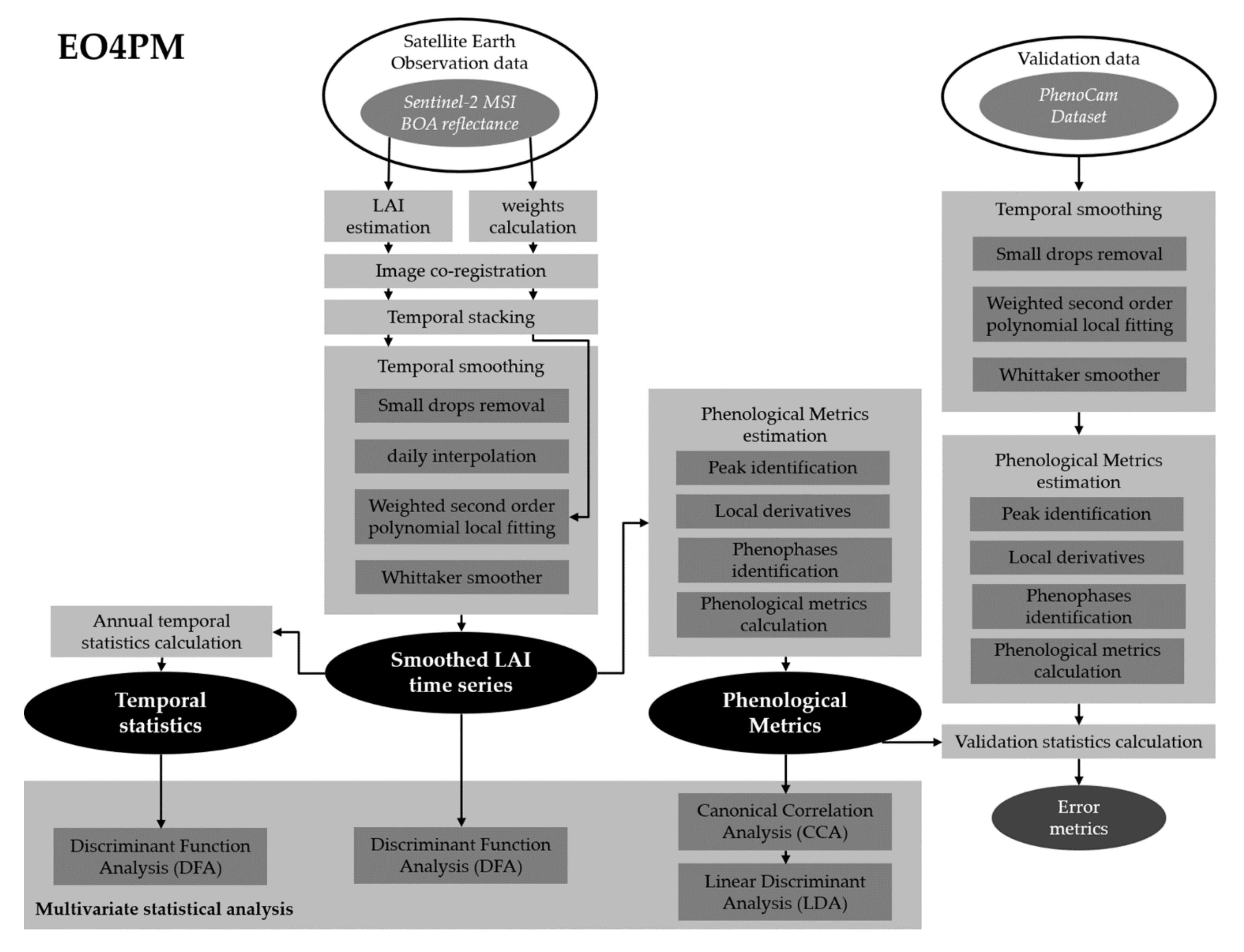
Figure 2 shows the overall data processing workflow. The LAI biophysical index, defined as half of the total green leaf area per unit ground surface area, was calculated from the S2 images using the biophysical processor [65,66] available in SNAP software version 7. From the LAI time series temporal variables were calculated, spatially co-registered using the AROSICS algorithm [67], in order to deal with weak spatial coherence of S2 time series processed using processing baselines 01.xx and 02.xx [68], and stacked in a large multidimensional datacube [68]. Then the LAI time series were temporally smoothed and daily interpolated. Complementary temporally explicit information defined “weights”, were generated in order to account for residual sub-pixel cloud contamination [69] and later updated during the data processing. weights values were derived from MSI B2 spectral band centered at 492 nm, and assigned following the rules: weights = 0.1 for B2 > 0.25; weights = 0.5 for B2 > 0.18 and B2 ≤ 0.25; weights = 1.0 for B2 ≤ 0.18.
The temporal smoothing and gap-filling aim to produce a vegetation index time series with evenly spaced timesteps, by means of a pixel-based approach consisting of four steps: (i) small drops removal; (ii) daily interpolation; (iii) weighted second-order polynomial local fitting; and (iv) Whittaker smoother. First, small drops in the temporal series were removed using a two-pass moving window filter. Daily interpolation was then performed with the R cran “stinepack” package [70], that use the Stineman algorithm [71] a method leading to much less tendency for “spurious” oscillations than traditional interpolation methods based on polynomials, such as splines. weights information was then updated with value “0.1”, assigned to interpolated missing values. Later, a weighted second-order polynomial local fitting using a moving window ranging over 7 non-missing temporal observations was used to apply a fine smoothing to the time series. The determination of weights for each time step in the time series, like the application of Savitsky–Golay filter, allows to produce an upper vegetation index envelope, reducing the small drops [72].
A first-order weighted Whittaker smoother [73,74] was finally applied in order to smooth the vegetation time series; in particular, the initial and final time series observation falling outside polynomial fitting local window, using the R cran ‘ptw’ package [75]. Lambda value used for the smoothing was set to 10 days, after performing a sensitivity analysis to tune this value and produce consistent results when smoothing time series with a different S2 revisit time of 2–3 days (multiple orbit acquisitions on few tiles) or 5–10 days (not shown).
After the smoothing procedure, the LAI daily time series were used to estimate the phenological metrics (Table 2) using the method described in [76]: the annual temporal statistics, specifically average (LAI_avg), minimum (LAI_min), maximum (LAI_max), delta (LAI_delta), standard deviation (LAI_std), and the seasonal temporal statistics, specifically winter average (LAI_djf_avg), winter minimum (LAI_djf_min), winter maximum (LAI_djf_max), summer average (LAI_jja_avg), summer minimum (LAI_jja_min), summer maximum (LAI_jja_max).
Plant phenology is characterized by phenophases that follow each other, from dormancy (or sowing in agriculture practices) through the start of season (characterized by the onset of greening with leaf unfolding), peak (or heading), maturity phase, flowering, senescence (characterized by curtailing of chlorophyll production that reveals various accessory pigments), leaf fall, and finally, dormancy.
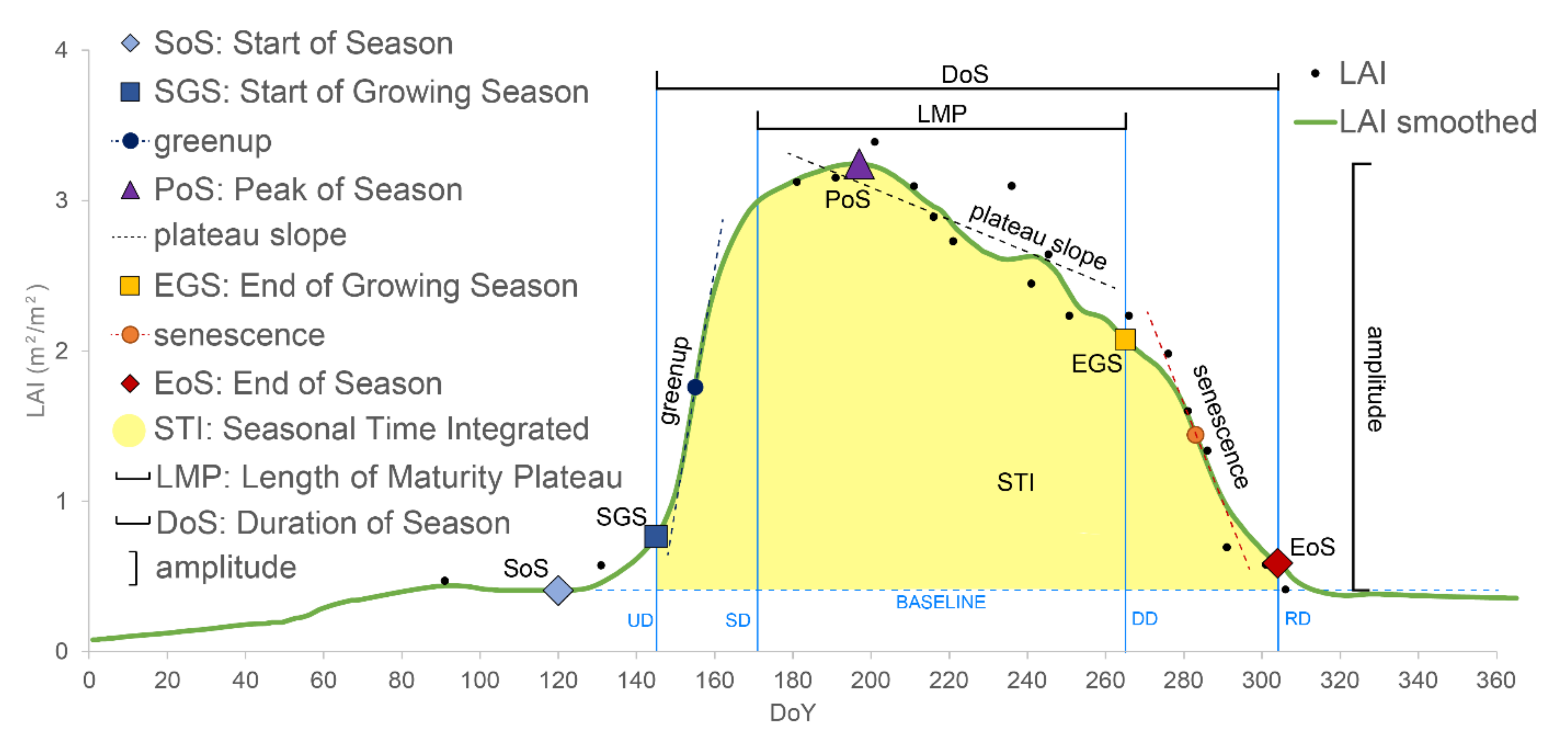
The method to estimate phenological metrics is based on a combination of local maxima in the first derivative [22,76] (Figure 3). It first identifies the vegetation peak, corresponding to absolute maximum time series value. Peak is used to initialize the identification of maximum increase (temporarily happening before the peak) and maximum decrease (temporarily happening after the peak) of time series first derivative. Maximum greenup rate (hereafter greenup) and maximum senescence rate (hereafter senescence) are defined as slopes of recovery and senescence lines tangent to the time series. The intersections among these lines and baseline and maxline identify the four phenophases in the original formulation (UD: upturn date; SD: stabilization date; DD: downturn date; RD: recession date) [76]. Starting from these phenophases, phenological metrics were extracted (Figure 3). Dates were expressed as absolute number of days (i.e., DoS and LMP phenological metrics) or as both calendar date and day of year (DoY).

2.5. Phenological Metrics Accuracy Assessment

In order to verify the accuracy of the estimated phenological metrics with ground phenology observations [51,77], the resulting S2 estimates were compared with the digital images of the PhenoCam network observations (https://phenocam.sr.unh.edu/webcam/, accessed on 11 March 2021) available for natural ecosystems in the study area (Figure 1, Table 3). The PhenoCam Dataset V2.0 is a fully processed, quality-controlled, and curated data set which is made freely available through the ORNL DAAC [78,79]. The daily 90th percentile of Green Chromatic Coordinate (GCC90), a vegetation index derived from PhenoCam photographic images that quantifies the greenness relative to the total brightness, has been used as reference time series and processed with the same procedure used to analyze S2 time series, starting from temporal smoothing processing step. Accuracy of the estimated phenological metrics was assesses by computing the Mean Error (ME), the Mean Absolute Error (MAE), the Root Mean Square Error (RMSE) and the correlation coefficient (r) between reference field data and S2 estimates. Since phenological metrics were derived from different time series (i.e., GCC90 and LAI), with a nonlinear relationship, only date estimates (expressed as DoY or absolute number of days) were compared for all the available PhenoCam time series in the period 2016–2020.
S2 acquisitions available in the period 2016–2020 were collected for location correspondent to PhenoCam sites, in order to generate multi-year time series for the comparison with ground observations.

2.6. Multivariate Analysis

Discriminant Function Analysis (DFA), Canonical Correlation Analysis (CCA) and Linear Discriminant Analysis (LDA) were selected to analyze the contribution of the three generated datasets (the smoothed vegetation curve, the temporal statistics, and the phenological metrics) to the characterization of forest habitat types (Table 1). The DFA is a statistical method that separates objects into classes by performing a multivariate analysis to highlight the differences among groups, namely the categorical response variable, and the variables needed to describe these differences, namely the predictors [80]. Four different forest habitat classes were considered for DFA analysis, corresponding to the broadleaved deciduous (T1), broadleaved evergreen (T2), needleleaved evergreen (T3) and needleleaved deciduous (T34) plant functional types. The CCA was used to explore the relationship between two sets of variables combining them in order to extract the variance of the data matrix by a limited number of independent axes (i.e., “canonical roots”, or “roots”) [81]. Linear Discriminant Analysis (LDA) is a dimensionality reduction technique, to reduce the number of dimensions in a dataset while retaining as much information as possible, providing the best possible separation between the groups [82].
The georeferenced points of vegetation plots were used to perform a spatial query over the variables generated from satellite time series, and precisely all the plots (14,385) over the smoothed vegetation curve and temporal statistics, and the T1 plots (8328) over the phenological metrics.
The data analysis was performed according to the following steps:
  • Regarding the smoothed vegetation curve and the temporal statistics variables (predictors), a DFA was executed to identify the variables able to discriminate the forest types (response variables) at the EUNIS II level;
  • As for the phenological metrics, a two steps analysis was performed for T1 EUNIS III level classes. Since the presence of two sets of variables, firstly a CCA was run on the phenological metrics dataset illustrated in Table 2 and constituted of 10 variables of LAI values and 9 variables of date values. The resulting independent and representative axes were then used to perform a LDA to discriminate the deciduous broadleaved forest types.
The analyses were performed using GDAL libraries, R programming language and libraries, QuantumGIS, SeNtinel Application Platform (SNAP), NetCDF Operators, and Climate Data Operators software.

3. Results

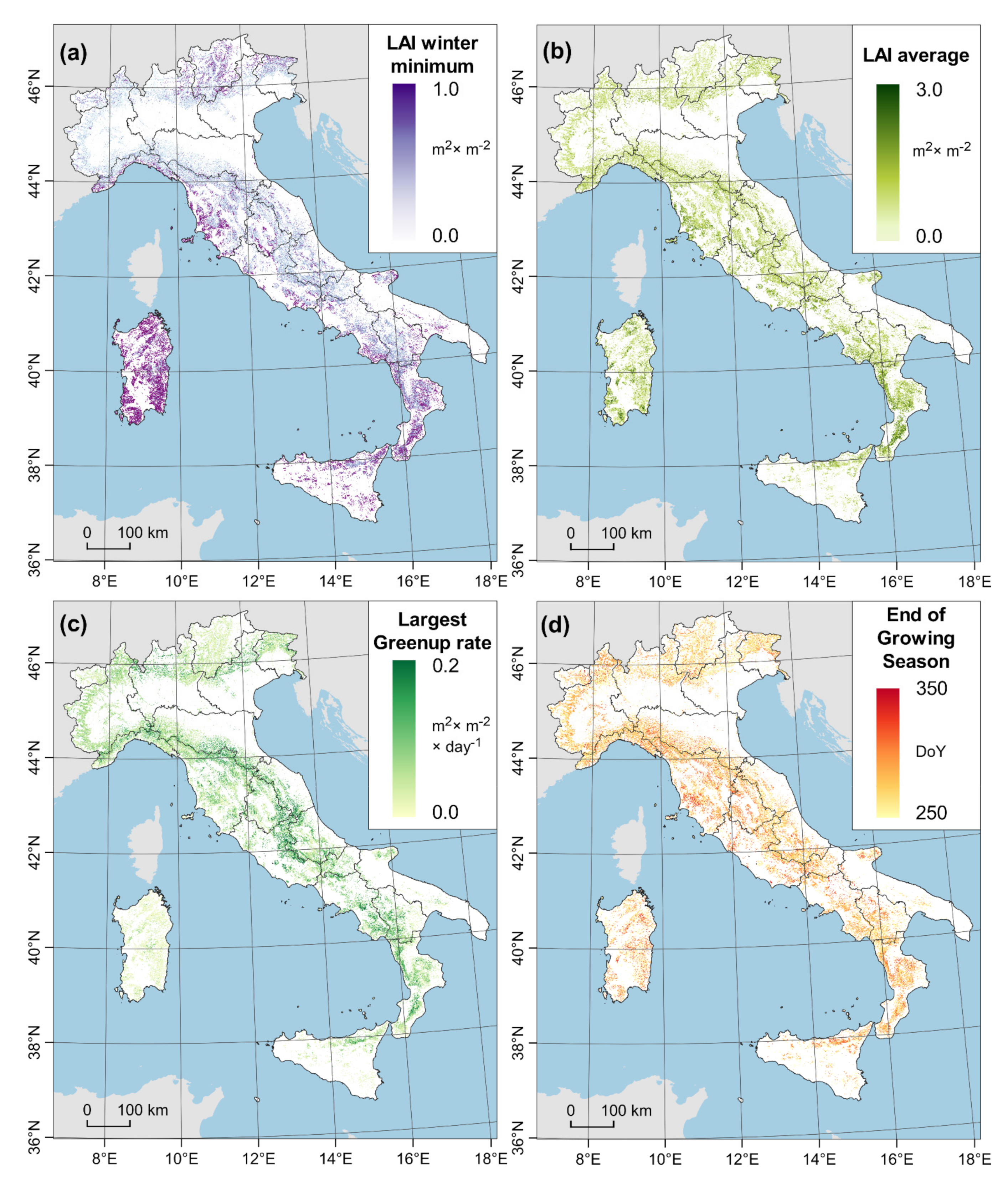
Figure 4 shows the spatial distribution maps of four phenological metrics estimated from S2 observations acquired during year 2019 for the Italian national territory. Temporal statistics related to LAI winter minimum (Figure 4a) clearly show higher values in the Alps region, corresponding to evergreen needleleaved forest (dominated by European Spruce, Silver Fir and Larch), and the distribution of evergreen broadleaved forests along the western coast of the peninsula (dominated by evergreen oaks), in southern regions and in Sardinia island. LAI average values (Figure 4b) show higher values for broadleaved forests and largest greenup rate (Figure 4c) is higher in central Apennines.
Results of the statistical analysis, conducted to compare the phenological metrics estimated from S2 time series with reference field data estimated from PhenoCam time series, located in the Alpine region, are reported in Table 4. Figure 5 shows the distribution of phenological metrics dates estimated from ground observation and from S2 time series.
Two EGS dates clusters can be observed in Figure 5, likely related to the differences between tree species and grasslands, the latter characterized by an early yellowing phase. PoS DoY estimated from S2 generally occurs later than the PhenoCam estimated one. This may be related to higher GCC90 signal saturation than LAI, and result in higher error metrics (Table 4) as compared to other assessed phenological metrics. Error metrics for DoS and LMP, estimated from a pair of phenological metrics estimates, may be higher than others due to the uncertainties in both greenup and senescence phenophases, that can increase error.
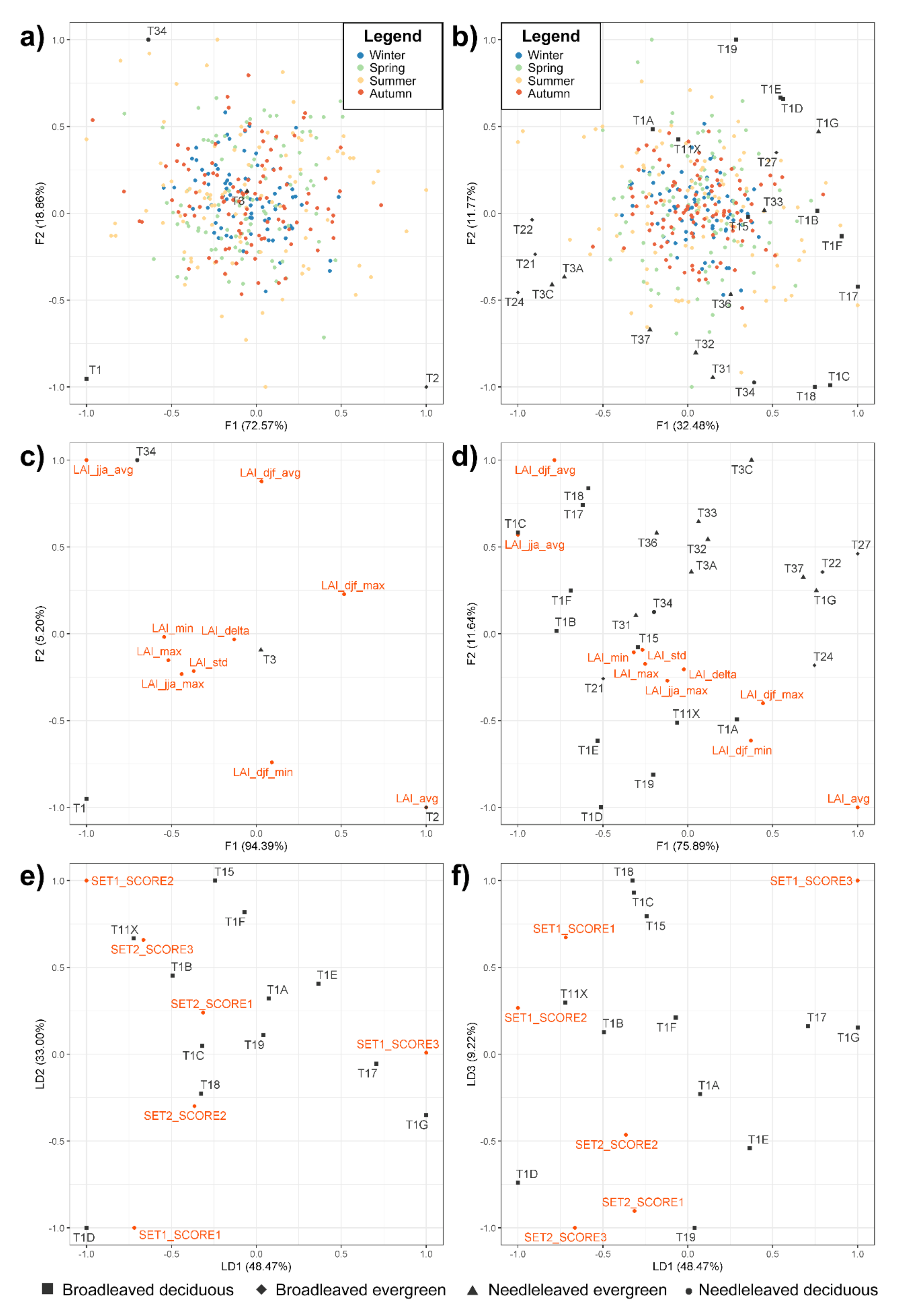
Figure 6 shows the results of multivariate analysis. Regarding the smoothed vegetation curve, the first two factors (F1 and F2) explain the 91.4% of the total variance (Figure 6a) for the EUNIS II level forest types and the 44.3% of the total variance for the EUNIS III level forest types (Figure 6b). In Figure 6a, the F1 (72.6% of the total variance) reveals a seasonal gradient with the deciduous forest types placed in the negative side of F1 and the evergreen in the positive one. The F2 instead (18.9% of the total variance) shows a differentiation of leaf types with the broadleaved located in the negative side of F2 and the needleleaved in the positive one. Figure 6b shows a similar separation between deciduous and evergreen alongside the F1, and broadleaved and needleleaved alongside F2, except for T33 (Mediterranean mountain Abies forest) that is a mixed forest type.
As for the temporal statistics, F1 and F2 explain the 99.6% of the total variance (Figure 6c) for the EUNIS II level forest types and the 87.5% of the total variance for the EUNIS III level forest types (Figure 6d). The distribution of the forest types with respect to the four quadrants of the DFA biplot is in line with what was reported for the LAI time series. Indeed, it is possible to recognize the same gradients in Figure 6c,d. Differently from the LAI time series biplots, that does not clearly express evident gradients, it is possible to find the contribution of the temporal statistics to the forest types discrimination. In Figure 6c, the F1 (94.4% of the total variance) reveals the summer productivity (LAI_max, LAI_jja, and LAI_std) and discriminates the deciduous forest types with T1 and T34 located in the negative side of the F1. T2, which represents the forest type with the maximum availability in terms of number of days of photosynthetic surface, is instead discriminated by LAI_avg and LAI_djf_max. The biplot of Figure 6d indicates a leaf-type productivity with T2 forest types located in the positive side of F1 (75.6% of the total variance) and in the negative side there are T3 and T1 forest types.
Regarding the phenological metrics, the output of the CCA consists of two sets of independent axes: SET1 axes for time values (DoY) and SET2 axes for LAI values. The results of the LDA are shown in Figure 6e,f. LD1 and LD2 explain the 81.5% of the total variance (Figure 6e), whereas LD2 and LD3 explain the 57.7% of the total variance (Figure 6f). In Figure 6e, LD1 (48.5% of the total variance) shows a temporal gradient with SET1_SCORE1, SET1_SCORE2, and SET1_SCORE3 that discriminate forest types characterized by a shorter growing season located in the right side of LD1. LD2 (33% of the total variance) is an expression of LAI values and discriminates the altitudinal gradient of broadleaved deciduous forests with beech and alder forest at the bottom of the biplot, and beech and oak at the top. Moreover, mesophilous forest types are located on the top side of the biplot. In Figure 6f, LD1 (48.5% of the total variance) shows a similar temporal gradient as in Figure 6e, whereas LD2 (9.2% of the total variance) indicates a latitudinal gradient with the alpine forest types located on the top side of the biplot (T18, T1C, and T15).
To sum up, a smoothed vegetation curve accounts for seasonal gradient and leaf type discrimination, whereas temporal statistics results, although showing the same gradients, enhance forest-type discrimination, highlighting forest productivity and leaf productivity features. Phenological metrics outcomes allow to enrich the information provided by the previous two analyses by associating a temporal gradient with specific phenophases that support forest-type distinction. Furthermore, altitudinal and latitudinal gradients also arise.

4. Discussion

Development of Earth observation data analytics allows to analyze and systematically extract diverse sets of information from a variety of large datasets, including those observing and measuring the response of environmental and ecosystem processes. Earth observation derived phenological metrics represent a promising tool to monitor ecological status, environmental conditions, climate change impacts on ecosystems, cropland practices, and more accurately forecast crop yields. Trends of phenological shifts in both spatial and temporal scales, with consequent impact on ecosystem functioning, could be identified using high resolution satellite derived phenological metrics.
Land-surface phenology has been estimated in the last decades from medium spatial resolution high revisit time satellite observations, that allow observing on regional to global scales but have a limited representativeness for phenological changes at ecosystem or species-level. S2 satellites, with a high spatial resolution and 5 days revisit time, opened the way to high resolution phenological metrics estimation, and represents a promising tool for a variety of ecological analyses, including for example the study of terrestrial ecosystems and species-specific phenology [22]. The LAI vegetation index estimated from satellite observations has been selected as source information to derive phenological metrics since it represents a biophysical parameter, and it is less affected by signal saturability in areas with high vegetation coverage. Alternatively, NIRv [83] and kNDVI [84] vegetation indices can be considered since they have low signal saturability in comparison to commonly used NDVI and EVI vegetation indices.
Retrieving plant phenology from time series of satellite Earth observation vegetation indices has been widely investigated and applied in the past two decades. USGS EROS and Copernicus initiatives [54,85] contributed to the development of operational products for landsurface phenology monitoring. TIMESAT, an algorithm implementing least-squares methods for processing time series of Earth Observation data, has been largely used to estimate phenophases. The implemented Savitzky–Golay filtering works very well with time series relatively unaffected by noise, while the asymmetric Gaussians, classified as semi-local method, force the data into the fixed functional form and they are able to follow also more complex behaviors, such as a rapid increase followed by a decreasing plateau [86]. The asymmetric Gaussian method has been found to be less sensitive to noise and to give better predictions for the beginnings and ends of the seasons [86]. The enhanced TIMESAT algorithm, using the third derivative, is relative stable in determining greenup and senescence, no matter whether vegetation index is changing quicker or slower [32].
Among the existing methodologies, the ones used in this study to temporally smooth time series and to estimate phenology metrics have been selected considering requirements and previous works in literature. The requirement for a generalized procedure, that can be applied to other vegetation indices and other satellite sensors, is the use of methods without any a priori information. Keeping smoothed temporal signal as close as possible to actual observations requires the use of a local curve fitting, to avoid an excessive simplification of the temporal curve methodologies and to allow less altered estimates for some of the phenological metrics (e.g., plateau_slope and STI). Finally, the use of a co-registration method to improve high spatial resolution satellite observations is advisable. The proposed procedure uses local curve fitting and local derivatives to identify phenophases, operating without thresholds or a priori information. Signal filtering is a very important processing step because it makes the vegetation time series interpretable to retrieve phenological information. The methodology temporally interpolates S2 time series in order to homogenize seasonal trajectories of vegetation indices. All the available satellite observations need to be optimally used, even if heavily hampered by clouds. In this study, the removal of invalid pixels (e.g., clouds, topographic shadows) prior the analysis assumes a key role in reducing factors affecting the quality of observations, that typically results in reducing vegetation indices values. The selection of S2 dataset with rigorous cloud detection algorithm [87], the use of weighted smoothing procedure and the temporal image co-registration enhance vegetation indices time series integrity.
Phenophases are estimated using the method presented in [76] and implemented in Phenopix R package, which offers a suite of standardized and reproducible processing code, designed for the extraction of phenological information from time-lapse digital photography of vegetation cover [22]. The method allows the extraction of greenup and senescence maximum rate date from time series smoothed using local curve fitting, diversely from other methodologies based on derivatives of the vegetation index seasonal trajectory that require extremely smoothed time series. The proposed approach distinguishes between Start of Season (SoS)–End of Season (EoS) and Start of Growing Season (SGS)–End of Growing Season (EGS) metrics, as compared to similar approaches. The start and the end of growing season is intended to represent seasonal bounds of photosynthetic tissues development phases. Diversely, the end of season comes at the end of the period of leaf-mineral nutrient remobilization during leaf senescence, when the plant is curtailing chlorophyll production revealing various accessory pigments, determining yellowing or browning of leaves, and consequently, driving the starting of fall foliage [61]. Vegetation normally changes more quickly during greenup than senescence [32], as noticeable from Figure 4. SoS phenological metric is of particular interest in the agriculture field since it represents the timing when vegetation index is at minimum before the onset of greenness. It should be related to pre-sowing plowing, a soil management practice that deals with soil preparation for a new crop, also utilized as post-harvest weed infestation control.
In forest ecosystems, minimum LAI is likely dependent on both evergreen overstory and/or understory species within a mixed-forest pixel [35]. The effect of deciduous understory species may affect surface reflectance very early in the growing season before growth of overstory canopy occurs. As a result, an early detection of onset of greenness for tree species within a mixed-forest pixel can be estimated [35]. To reduce such effect, amplitude metric is computed considering the difference between vegetation peak and vegetation baseline, in order to eliminate the effect of evergreen species on the minimum vegetation index value.
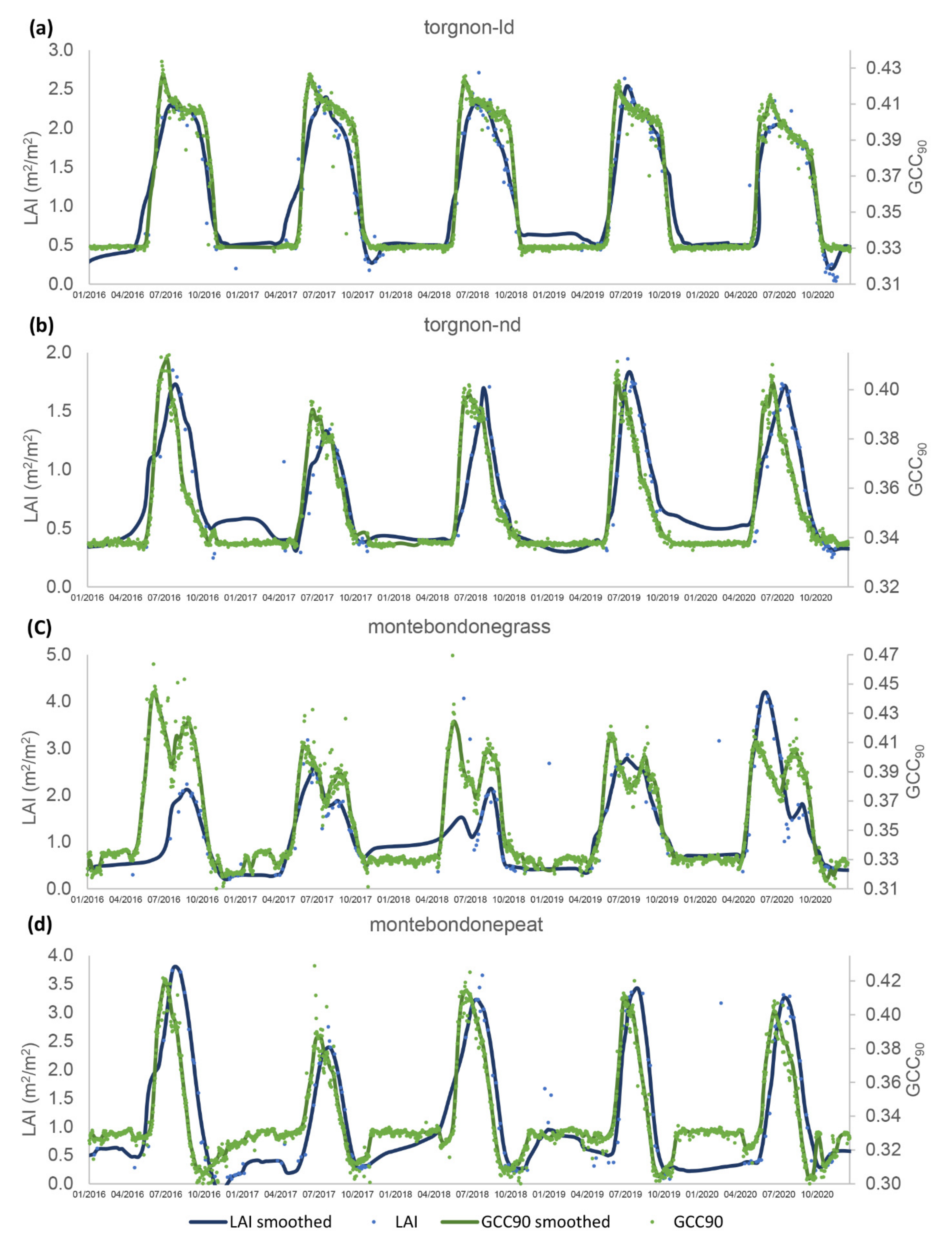
The association between the estimated phenological metrics dates and ground observations was evaluated. To assess the accuracy of the phenological retrievals, ground-truth information on phenological transition dates would be required [88]. Although subjective ocular estimates were shown to have a close match to remote sensing indices, they are time-consuming as they require the frequent presence of an observer in the field [89]. To overcome this, the use of digital cameras that automatically take several pictures per day, with a strong focus on forest ecosystems [21], allows to collect time series of greenness chromatic coordinates, that can then be subjected to similar phenology extraction methods as for satellite imagery to identify phenological transition dates [22]. Validating phenology metrics derived from satellite data product may be difficult due to vegetation heterogeneity [32]. Data quality and phenology retrieval methods can be source of uncertainties in phenological metrics estimates [90], and its accuracy remains to be validated globally. Error metrics calculated using ground observations resulted in a MAE of about 15 days for the various metrics analyzed. This is consistent with accuracy reported in other studies [34,91] and can be caused by many error sources. For example, the use of different indices to estimate phenological metrics, LAI and GCC90 with the latter more affected by signal saturability (Figure A1), may have contributed to generate differences in the estimated values. In fact, previous research studies demonstrated that phenological metrics derived from NDVI and EVI for the same geographic area are not in 100% agreement with each other [32].
Forest plant communities, together with their own typical floristic composition, show exclusive phenological dynamics recognizable by vegetation indices time series [42]. Both vegetation indices time series [42,61] and land surface phenological metrics [61,92] has been successfully used to classify plant communities and natural habitats, discriminating vegetation patterns dominated by species with similar phenology features. Multivariate statistical analysis conducted in this research study allowed to understand how the three generated datasets (the smoothed vegetation curve, the temporal statistics, and the phenological metrics) have the capacity to serve as temporal discriminants to detect forest ecosystems processes responses to environmental gradients. Results from multivariate analysis demonstrate how temporal statistics and phenological metrics are representative of the time-related variability, can synthetize key information from satellite time series, reducing data dimensionality, and thus can be used as temporal discriminants for forest ecosystems classification and mapping. Specifically, smoothed vegetation curve and temporal statistics are able to highlight seasonal gradient and leaf-type characteristics to discriminate forest types, with additional information about forest and leaf productivity provided by temporal statistics analysis. Furthermore, temporal, altitudinal, and latitudinal gradients are obtained from phenological metrics analysis, which also allows to associate temporal gradient with specific phenophases. High spatial resolution smoothed time series and phenological metrics open up to the provision of novel temporal information about forest phenology anomalies and useful monitoring system to scrutinize spatio-temporal patterns of forest disturbance [62].
In the frame of ecosystem monitoring (e.g., conservation status), and specifically for grassland management in agricultural areas (e.g., fodder), the systematic capturing of cutting times would be highly relevant for the surveillance of areas granted by EU funding programmes [93], under policies on rural development through funding and actions (EU’s Common Agricultural Policy-PAC). The capacity of mapping crop types using high spatial resolution phenological metrics estimated using the proposed procedure has been demonstrated in [94] for heterogeneous, small, and fragmented agricultural systems. In the context of crop-type mapping and the monitoring of agricultural practices, synthesizing information to fewer phenological metrics would facilitate image data processing, for example, image segmentation by reducing time series dimensionality.
While inter-annual variability of phenological metrics can be evaluated even at a local scale, and analysis on continental scales can detect spatial variability in phenology across climate gradients. In fact, vegetation phenology is highly sensitive to climate conditions and is a climate change fingerprint [15]. Warm and cold spells, which are not single extreme events but can be regarded as a compound extreme, such as a persistence of weather conditions, have impacts on the onset of phenological seasons, that differed strongly depending on species, phase and timing of the event [15]. Phenology also controls many feedbacks of vegetation to the climate system by influencing the seasonality of albedo, surface roughness length, canopy conductance, and fluxes of water, energy, CO2 and biogenic volatile organic compounds [95]. Knowledge of how geo-morphological and bio-climatical conditions affect phenological behavior is valuable information to model the potential effects of climate change and to estimate the future adaptation of plant growing in different geographical areas.
The proposed approach has been demonstrated using S2 LAI time series. Other vegetation indices and other satellite sensors or virtual constellation of sensors can be used to estimate phenological metrics with the presented procedure. New perspectives concerning monitoring of plant phenology can benefit from dense time series generated from virtual constellations, such as the Harmonized Landsat and Sentinel-2 (HLS) dataset initiative, or synergies with Synthetic Aperture Radar (SAR) sensors satellite observations. SAR time series have a strong seasonal signal in VH radar backscattering coefficient [96], as well as the ratio between VV and VH coefficients, that allows the monitoring of phenology in deciduous forests independently of the cloud cover [97].

5. Conclusions

Earth observation derived phenological metrics to represent a promising tool to monitor ecological status, environmental conditions, climate change impacts on ecosystems, cropland practices, and more accurately forecast crop yields. The proposed automated and transferable procedure combines available validated methodologies to exploit full satellite Earth observation time series without any a priori information, to produce rapid and updated information about plant phenology. Estimated phenological metrics have been validated using in situ PhenoCam observations with satisfactory results.
This study shows that integrated data and methodologies based on plant phenology may be an effective tool to generate Earth Observation derived temporal discriminants, very useful to characterize forest ecosystems, and may help the processes of vegetation recognition and classification, in addition to support monitoring activities of natural ecosystems and agro-forestry systems.

Author Contributions

Conceptualization, F.F. and D.S.; methodology, F.F. and D.S.; software, F.F.; validation, F.F.; formal analysis, F.F. and D.S.; investigation, F.F. and E.A.; data curation, F.F. and E.A.; writing—original draft preparation, F.F. and D.S.; writing—review and editing, F.F., D.S. and E.A. All authors have read and agreed to the published version of the manuscript.

Funding

This manuscript is not funded by a specific project grant.

Institutional Review Board Statement

Not applicable.

Informed Consent Statement

Not applicable.

Acknowledgments

The authors want to acknowledge the Italian Institute for Environmental Protection and Research (ISPRA) that under the research agreement with the Italian Space Agency (ASI) “Habitat Mapping project” and “Air Quality project” stimulated further development of the results presented in this study. The authors are grateful to colleagues Sofia Bajocco and Luca Salvati for useful and constructive comments and suggestions, and to colleague Mirco Boschetti for triggering research interest into remote sensing phenology topic. We acknowledge macrovector for providing free vector image through freepik.com (accessed on 22 December 2021). Moreover, authors are grateful to the many individuals working on the development of free and open-source software for supporting the sharing of knowledge.

Conflicts of Interest

The authors declare no conflict of interest.

Appendix A

Figure A1. Comparison of PhenoCam GCC90 time series with the corresponding S2 LAI time series for the period 2016–2020 in the four Italian PhenoCam sites. (a) torgnon-ld site; (b) torgnon-nd site; (c) montebondonegrass site; (d) montebondonepeat site.
Remotesensing 14 00721 g0a1

References

  1. Betancourt, J.L.; Schwartz, M.D.; Breshears, D.D.; Brewer, C.A.; Frazer, G.; Gross, J.E.; Mazer, S.J.; Reed, B.C.; Wilson, B.E. Evolving plans for the USA National Phenology Network. Eos Trans. AGU 2007, 88, 211. [Google Scholar] [CrossRef]
  2. Van Vliet, A.J.H.; de Groot, R.S.; Bellens, Y.; Braun, P.; Bruegger, R.; Bruns, E.; Clevers, J.; Estreguil, C.; Flechsig, M.; Jeanneret, F.; et al. The European Phenology Network. Int. J. Biometeorol. 2003, 47, 202–212. [Google Scholar] [CrossRef] [PubMed]
  3. Nasahara, K.N.; Nagai, S. Review: Development of an in situ observation network for terrestrial ecological remote sensing: The Phenological Eyes Network (PEN). Ecol. Res. 2015, 30, 211–223. [Google Scholar] [CrossRef]
  4. Templ, B.; Koch, E.; Bolmgren, K.; Ungersböck, M.; Paul, A.; Scheifinger, H.; Busto, M.; Chmielewski, F.M.; Hájková, L.; Hodzic, S. Pan European Phenological database (PEP725): A single point of access for European data. Int. J. Biometeorol. 2018, 62, 1109–1113. [Google Scholar] [CrossRef]
  5. Lieth, H. Phenology and Seasonality Modeling; Springer: Berlin/Heidelberg, Germany, 1974. [Google Scholar]
  6. Baddour, O.; Kontongomde, H. Guidelines for Plant Phenological Observations; WMO-TD No. 1484; World Meteorological Organization: Geneva, Switzerland, 2009. [Google Scholar]
  7. Schwartz, M.D. Phenology: An Integrative Environmental Science; Springer: Dordrecht, The Netherlands, 2013. [Google Scholar]
  8. IPCC (Intergovernmental Panel on Climate Change). Climate Change 2001: The Scientific Basis. Contribution of Working Group I to the Third Assessment Report of the Intergovernmental Panel on Climate Change; Houghton, J.T., Ding, Y., Griggs, D.J., Noguer, M., van der Linden, P.J., Dai, X., Maskell, K., Johnson, C.A., Eds.; Cambridge University Press: New York, NY, USA, 2001. [Google Scholar]
  9. Myneni, R.B.; Keeling, C.D.; Tucker, C.J.; Asrar, G.; Nemani, R.R. Increased plant growth in the northern high latitudes from 1981 to 1991. Nature 1997, 386, 698–702. [Google Scholar] [CrossRef]
  10. Walkovszky, A. Changes in phenology of the locust tree (Robinia pseudoacacia L) in Hungary. Int. J. Biometeorol. 1998, 41, 155–160. [Google Scholar] [CrossRef]
  11. Chmielewski, F.M.; Roetzer, T. Phenological trends in Europe in relation to climatic changes. Agrarmeteorol. Schr. 2000, 7, 1–15. [Google Scholar]
  12. Schwartz, M.D.; Reiter, B.E. Changes in North American spring. Int. J. Climatol. 2000, 20, 929–932. [Google Scholar] [CrossRef]
  13. Menzel, A.; Estrella, N.; Fabian, P. Spatial and temporal variability of the phenological seasons in Germany from 1951–1996. Global Change Biol. 2001, 7, 657–666. [Google Scholar] [CrossRef]
  14. Brown, M.E.; de Beurs, K.M. The response of African land surface phenology to large scale climate oscillations. Remote Sens. Environ. 2010, 10, 2286–2296. [Google Scholar] [CrossRef] [Green Version]
  15. Menzel, A.; Seifert, H.; Estrella, N. Effects of recent warm and cold spells on European plant phenology. Int. J. Biometeorol. 2011, 55, 921–932. [Google Scholar] [CrossRef]
  16. Noormets, A. Phenology of Ecosystem Processes; Springer: New York, NY, USA, 2009. [Google Scholar]
  17. Visser, M.E.; Caro, S.P.; van Oers, K.; Schaper, S.V.; Helm, B. Phenology, seasonal timing and circannual rhythms: Towards a unified framework. Philosoph. Trans. R. Soc. B—Biol. Sci. 2010, 365, 3113–3127. [Google Scholar] [CrossRef] [PubMed] [Green Version]
  18. Menzel, A.; Sparks, T.; Estrella, N.; Koch, E.; Aasa, A.; Ahas, R.; Alm-Kübler, K.; Bissolli, P.; Braslavská, O.; Briede, A.; et al. European phenological response to climate change matches the warming pattern. Glob. Change Biol. 2006, 12, 1969–1976. [Google Scholar] [CrossRef]
  19. Menzel, A.; Dose, V. Analysis of long-term time-series of beginning of flowering by Bayesian function estimation. Meteorologische Zeitschrift 2005, 14, 429–434. [Google Scholar] [CrossRef] [Green Version]
  20. Meier, U.; Bleiholder, H.; Buhr, L.; Feller, C.; Hack, H.; Hess, M.; Lancashire, P.D.; Schnock, U.; Stauss, R.; van den Boom, T.; et al. The BBCH system to coding the phenological growth stages of plants—History and publications. J. für Kulturpflanzen 2009, 61, 41–52. [Google Scholar] [CrossRef]
  21. Morisette, J.T.; Richardson, A.D.; Knapp, A.K.; Fisher, J.I.; Graham, E.A.; Abatzoglou, J.; Wilson, B.E.; Breshears, D.D.; Henebry, G.M.; Hanes, J.M.; et al. Tracking the rhythm of the seasons in the face of global change: Phenological research in the 21st Century. Front. Ecol. Environ. 2009, 7, 253–260. [Google Scholar] [CrossRef] [Green Version]
  22. Filippa, G.; Cremonese, E.; Migliavacca, M.; Galvagno, M.; Forkel, M.; Wingate, L.; Tomelleri, E.; Morra di Cella, U.; Richardson, A.D. Phenopix: AR package for image-based vegetation phenology. Agric. For. Meteorol. 2016, 220, 141–150. [Google Scholar] [CrossRef] [Green Version]
  23. Bajocco, S.; Raparelli, E.; Teofili, T.; Bascietto, M.; Ricotta, C. Text Mining in Remotely Sensed Phenology Studies: A Review on Research Development, Main Topics, and Emerging Issues. Remote Sens. 2019, 11, 2751. [Google Scholar] [CrossRef] [Green Version]
  24. Jeong, S.J.; Ho, C.H.; Gim, H.J.; Brown, M.E. Phenology shifts at start vs. end of growing season in temperate vegetation over the Northern Hemisphere for the period 1982–2008. Glob. Change Biol. 2011, 17, 2385–2399. [Google Scholar] [CrossRef]
  25. Zeng, L.; Wardlow, B.; Xiang, D.; Hu, S.; Li, D. A review of vegetation phenological metrics extraction using time-series, multispectral satellite data. Remote Sens. Environ. 2020, 237, 111511. [Google Scholar] [CrossRef]
  26. USA-NPN National Phenology Network. Land Surface Phenology and Remote Sensing (LSP/RS). Available online: https://usanpn.org/node/14 (accessed on 21 November 2021).
  27. De Beurs, K.M.; Henebry, G.M. Land surface phenology and temperature variation in the International Geosphere–Biosphere Program high-latitude transects. Glob. Change Biol. 2005, 11, 779–790. [Google Scholar] [CrossRef]
  28. Roy, D.P.; Lewis, P.; Schaaf, C.; Devadiga, S.; Boschetti, L. The global impact of cloud on the production of MODIS bi-directional reflectance model based composites for terrestrial monitoring. IEEE Geosci. Remote Sens. Lett. 2006, 3, 452–456. [Google Scholar] [CrossRef] [Green Version]
  29. Duchemin, B.; Goubier, J.; Courrier, G. Monitoring phenological key stages and cycle duration of temperate deciduous forest ecosystems with NOAA/AVHRR data. Remote Sens. Environ. 1999, 67, 68–82. [Google Scholar] [CrossRef]
  30. Heumann, B.W.; Seaquist, J.W.; Eklundh, L.; Jönsson, P. AVHRR derived phenological change in the Sahel and Soudan, Africa, 1982–2005. Remote Sens. Environ. 2007, 108, 385–392. [Google Scholar] [CrossRef]
  31. Zhang, X.; Friedl, M.A.; Schaaf, C.B.; Strahler, A.H.; Hodges, J.C.F.; Gao, F.; Reed, B.C.; Huete, A. Monitoring vegetation phenology using MODIS. Remote Sens. Environ. 2003, 84, 471–475. [Google Scholar] [CrossRef]
  32. Tan, B.; Morisette, J.T.; Wolfe, R.E.; Gao, F.; Ederer, G.A.; Nightingale, J.; Pedelty, J.A. An enhanced TIMESAT algorithm for estimating vegetation phenology metrics from MODIS data. IEEE J. Sel. Top. Appl. Earth Observ. Remote Sens. 2010, 4, 361–371. [Google Scholar] [CrossRef]
  33. Li, J.; Roy, D.P. A Global Analysis of Sentinel-2A, Sentinel-2B and Landsat-8 Data Revisit Intervals and Implications for Terrestrial Monitoring. Remote Sens. 2017, 9, 902. [Google Scholar] [CrossRef] [Green Version]
  34. Vrieling, A.; Meroni, M.; Darvishzadeh, R.; Skidmore, A.K.; Wang, T.; Zurita-Milla, R.; Oosterbeek, K.; O’Connor, B.; Paganini, M. Vegetation phenology from Sentinel-2 and field cameras for a Dutch barrier island. Remote Sens. Environ. 2018, 215, 517–529. [Google Scholar] [CrossRef]
  35. Kang, S.; Running, S.W.; Lim, J.H.; Zhao, M.; Park, C.R.; Loehman, R. A regional phenology model for detecting onset of greenness in temperate mixed forests, Korea: An application of MODIS leaf area index. Remote Sens. Environ. 2003, 86, 232–242. [Google Scholar] [CrossRef]
  36. Verhegghen, A.; Bontemps, S.; Defourny, P. A global NDVI and EVI reference data set for land-surface phenology using 13 years of daily SPOT-VEGETATION observations. Int. J. Remote Sens. 2014, 35, 2440–2471. [Google Scholar] [CrossRef] [Green Version]
  37. Wu, C.; Peng, D.; Soudani, K.; Siebicke, L.; Gough, C.M.; Arain, M.A.; Bohrer, G.; Lafleur, P.M.; Peichl, M.; Gonsamo, A. Land surface phenology derived from normalized difference vegetation index (NDVI) at global FLUXNET sites. Agric. For. Meteorol. 2017, 233, 171–182. [Google Scholar] [CrossRef]
  38. White, M.A.; Hoffman, F.M.; Hargrove, W.W.; Nemani, R.R. A global framework for monitoring phenological responses to climate change. Geophys. Res. Lett. 2005, 32, L04705. [Google Scholar] [CrossRef] [Green Version]
  39. Hargrove, W.W.; Spruce, J.P.; Gasser, G.E.; Hoffman, F.M. Toward a national early warning system for forest disturbances using remotely sensed canopy phenology. Photogramm. Eng. Remote Sens. 2009, 75, 1150–1156. [Google Scholar]
  40. Boschetti, M.; Nelson, A.; Nutini, F.; Manfron, G.; Busetto, L.; Barbieri, M.; Laborte, A.; Raviz, J.; Holecz, F.; Mabalay, M.R.O.; et al. Rapid Assessment of Crop Status: An Application of MODIS and SAR Data to Rice Areas in Leyte, Philippines Affected by Typhoon Haiyan. Remote Sens. 2015, 7, 6535–6557. [Google Scholar] [CrossRef] [Green Version]
  41. Bajocco, S.; Ferrara, C.; Alivernini, A.; Bascietto, M.; Ricotta, C. Remotely-sensed phenology of Italian forests: Going beyond the species. Int. J. Appl. Earth Obs. Geoinf. 2019, 74, 314–321. [Google Scholar] [CrossRef]
  42. Pesaresi, S.; Mancini, A.; Casavecchia, S. Recognition and Characterization of Forest Plant Communities through Remote-Sensing NDVI Time Series. Diversity 2020, 12, 313. [Google Scholar] [CrossRef]
  43. Valero, S.; Morin, D.; Inglada, J.; Sepulcre, G.; Arias, M.; Hagolle, O.; Dedieu, G.; Bontemps, S.; Defourny, P.; Koetz, B. Production of a Dynamic Cropland Mask by Processing Remote Sensing Image Series at High Temporal and Spatial Resolutions. Remote Sens. 2016, 8, 55. [Google Scholar] [CrossRef] [Green Version]
  44. Boschetti, M.; Busetto, L.; Manfron, G.; Laborte, A.; Asilo, S.; Pazhanivelan, S.; Nelson, A. PhenoRice: A method for automatic extraction of spatio-temporal information on rice crops using satellite data time series. Remote Sens. Environ. 2017, 194, 347–365. [Google Scholar] [CrossRef] [Green Version]
  45. Reed, B.C.; Brown, J.F.; VanderZee, D.; Loveland, T.R.; Merchant, J.W.; Ohlen, D.O. Measuring phenological variability from satellite data. J. Veg. Sci. 1994, 5, 703–714. [Google Scholar] [CrossRef]
  46. Gu, Y.; Brown, J.F.; Miura, T.; van Leeuwen, W.J.D.; Reed, B.C. Phenological Classification of the United States: A Geographic Framework for Extending Multi-Sensor Time-Series Data. Remote Sens. 2010, 2, 526–544. [Google Scholar] [CrossRef] [Green Version]
  47. Clerici, N.; Weissteiner, C.J.; Gerard, F. Exploring the Use of MODIS NDVI-Based Phenology Indicators for Classifying Forest General Habitat Categories. Remote Sens. 2012, 4, 1781–1803. [Google Scholar] [CrossRef] [Green Version]
  48. White, M.A.; Thornton, P.E.; Running, S.W. A continental phenology model for monitoring vegetation responses to interannual climatic variability. Glob. Biogeochem. Cycles 1997, 11, 217–234. [Google Scholar] [CrossRef]
  49. Curnel, Y.; Oger, R. Agrophenology Indicators from Remote Sensing: State of the Art. Available online: https://www.isprs.org/proceedings/XXXVI/8-W48/ (accessed on 22 December 2021).
  50. De Beurs, K.M.; Henebry, G.M. Spatio-Temporal Statistical Methods for Modeling Land Surface Phenology. In Phenological Research: Methods for Environmental and Climate Change Analysis; Hudson, I.L., Keatley, M.R., Eds.; Springer: Dordrecht, The Netherlands, 2010; pp. 177–208. [Google Scholar] [CrossRef]
  51. Xu, H.; Twine, T.E.; Yang, X. Evaluating Remotely Sensed Phenological Metrics in a Dynamic Ecosystem Model. Remote Sens. 2014, 6, 4660–4686. [Google Scholar] [CrossRef] [Green Version]
  52. Matongera, T.N.; Mutanga, O.; Sibanda, M.; Odindi, J. Estimating and Monitoring Land Surface Phenology in Rangelands: A Review of Progress and Challenges. Remote Sens. 2021, 13, 2060. [Google Scholar] [CrossRef]
  53. European Environment Agency (EEA). High Resolution Vegetation Phenology and Productivity (HR-VPP), Seasonal Trajectories and VPP parameters; Copernicus Land Monitoring Service, European Environment Agency: Copenhagen, Denmark, 2021. [Google Scholar]
  54. High Resolution Vegetation Phenology and Productivity. Available online: https://land.copernicus.eu/pan-european/biophysical-parameters/high-resolution-vegetation-phenology-and-productivity (accessed on 22 December 2021).
  55. Tian, F.; Cai, Z.; Jin, H.; Hufkens, K.; Scheifinger, H.; Tagesson, T.; Smets, B.; Van Hoolst, R.; Bonte, K.; Ivits, E.; et al. Calibrating vegetation phenology from Sentinel-2 using eddy covariance, PhenoCam, and PEP725 networks across Europe. Remote Sens. Environ. 2021, 260, 112456. [Google Scholar] [CrossRef]
  56. Pesaresi, S.; Galdenzi, D.; Biondi, E.; Casavecchia, S. Bioclimate of Italy: Application of the worldwide bioclimatic classification system. J. Maps 2014, 10, 538–553. [Google Scholar] [CrossRef]
  57. Copertura del Suolo. Available online: https://www.isprambiente.gov.it/it/attivita/suolo-e-territorio/copertura-del-suolo (accessed on 22 December 2021).
  58. Chytrý, M.; Hennekens, S.M.; Jiménez-Alfaro, B.; Knollová, I.; Dengler, J.; Jansen, F.; Landucci, F.; Schaminée, J.H.; Acìc, S.; Agrillo, E.; et al. European Vegetation Archive (EVA): An integrated database of European vegetation plots. Appl. Veg. Sci. 2016, 19, 173–180. [Google Scholar] [CrossRef] [Green Version]
  59. Agrillo, E.; Alessi, N.; Massimi, M.; Spada, F.; De Sanctis, M.; Francesconi, F.; Cambria, V.E.; Attorre, F. Nationwide Vegetation Plot Database-Sapienza University of Rome: State of the art, basic figures and future perspectives. Phytocoenologia 2017, 47, 221–222. [Google Scholar] [CrossRef]
  60. Chytrý, M.; Tichý, L.; Hennekens, S.M.; Knollová, I.; Janssen, J.A.; Rodwell, J.S.; Peterka, T.; Marcenò, C.; Landucci, F.; Dani-helka, J.; et al. EUNIS Habitat Classification: Expert system, characteristic species combinations and distribution maps of European habitats. Appl. Veg. Sci. 2020, 23, 648–675. [Google Scholar] [CrossRef]
  61. Agrillo, E.; Filipponi, F.; Pezzarossa, A.; Casella, L.; Smiraglia, D.; Orasi, A.; Attorre, F.; Taramelli, A. Earth Observation and Biodiversity Big Data for Forest Habitat Types Classification and Mapping. Remote Sens. 2021, 13, 1231. [Google Scholar] [CrossRef]
  62. Löw, M.; Koukal, T. Phenology Modelling and Forest Disturbance Mapping with Sentinel-2 Time Series in Austria. Remote Sens. 2020, 12, 4191. [Google Scholar] [CrossRef]
  63. Hagolle, O.; Huc, M.; Desjardins, C.; Auer, S.; Richter, R. MAJA Algorithm Theoretical Basis Document; CNES: Paris, France, 2017. [Google Scholar] [CrossRef]
  64. Rouquié, B.; Hagolle, O.; Bréon, F.M.; Boucher, O.; Desjardins, C.; Rémy, S. Using Copernicus atmosphere monitoring service products to constrain the aerosol type in the atmospheric correction processor MAJA. Remote Sens. 2017, 9, 1230. [Google Scholar] [CrossRef] [Green Version]
  65. Weiss, M.; Baret, F. S2 ToolBox Level 2 Products: LAI, FAPAR, FCOVER. 2016. Available online: https://step.esa.int/docs/extra/ATBD_S2ToolBox_L2B_V1.1.pdf (accessed on 21 November 2021).
  66. Djamai, N.; Fernandes, R.; Weiss, M.; McNairn, H.; Goïta, K. Validation of the Sentinel Simplified Level 2 Product Prototype Processor (SL2P) for mapping cropland biophysical variables using Sentinel-2/MSI and Landsat-8/OLI data. Remote Sens. Environ. 2019, 225, 416–430. [Google Scholar] [CrossRef]
  67. Scheffler, D.; Hollstein, A.; Diedrich, H.; Segl, K.; Hostert, P. AROSICS: An Automated and Robust Open-Source Image Co-Registration Software for Multi-Sensor Satellite Data. Remote Sens. 2017, 9, 676. [Google Scholar] [CrossRef] [Green Version]
  68. Filipponi, F. Exploitation of Sentinel-2 Time Series to Map Burned Areas at the National Level: A Case Study on the 2017 Italy Wildfires. Remote Sens. 2019, 11, 622. [Google Scholar] [CrossRef] [Green Version]
  69. Manfron, G.; Crema, A.; Boschetti, M.; Confalonieri, R. Testing Automatic Procedures to Map Rice Area and Detect Phenological Crop Information Exploiting Time Series Analysis of Remote Sensed MODIS Data. In Remote Sensing for Agriculture, Ecosystems, and Hydrology XIV, Proceedings of the SPIE 8531, Edinburgh, UK, 24–26 September 2012; Society of Photo-Optical Instrumentation Engineers (SPIE): Bellingham, WA, USA, 2012; Volume 8531, p. 85311E. [Google Scholar] [CrossRef]
  70. Johannesson, T.; Bjornsson, H. Stinepack: Stineman, a Consistently Well Behaved Method of Interpolation. R Package Version 1.3. 2012. Available online: https://CRAN.R-project.org/package=stinepack (accessed on 21 November 2021).
  71. Stineman, R.W. A Consistently Well Behaved Method of Interpolation. Creat. Comput. 1980, 6, 54–57. [Google Scholar]
  72. Chen, J.; Jönsson, P.; Tamura, M.; Gu, Z.; Matsushita, B.; Eklundh, L. A simple method for reconstructing a high-quality NDVI time-series data set based on the Savitzky-Golay filter. Remote Sens. Environ. 2004, 91, 332–344. [Google Scholar] [CrossRef]
  73. Whittaker, E.T. On a new method of graduation. Proc. Edinb. Math. Soc. 1923, 41, 63–75. [Google Scholar] [CrossRef] [Green Version]
  74. Eilers, P.H. A perfect smoother. Anal. Chem. 2003, 75, 3631–3636. [Google Scholar] [CrossRef]
  75. Bloemberg, T.G.; Gerretzen, J.; Wouters, H.J.; Gloerich, J.; van Dael, M.; Wessels, H.J.; van den Heuvel, L.P.; Eilers, P.H.C.; Buydens, L.M.C.; Wehrens, R. Improved parametric time warping for proteomics. Chemom. Intell. Lab. Syst. 2010, 104, 65–74. [Google Scholar] [CrossRef]
  76. Gu, L.; Post, W.M.; Baldocchi, D.D.; Black, T.A.; Suyker, A.E.; Verma, S.B.; Vesala, T.; Wofsy, S.C. Characterizing the Seasonal Dynamics of Plant Community Photosynthesis Across a Range of Vegetation Types. In Phenology of Ecosystem Processes; Noormets, A., Ed.; Springer: Berlin/Heidelberg, Germany, 2009; pp. 35–58. [Google Scholar] [CrossRef] [Green Version]
  77. Huang, X.; Liu, J.; Zhu, W.; Atzberger, C.; Liu, Q. The Optimal Threshold and Vegetation Index Time Series for Retrieving Crop Phenology Based on a Modified Dynamic Threshold Method. Remote Sens. 2019, 11, 2725. [Google Scholar] [CrossRef] [Green Version]
  78. Richardson, A.D.; Hufkens, K.; Milliman, T.; Aubrecht, D.M.; Chen, M.; Gray, J.M.; Johnston, M.R.; Keenan, T.F.; Klosterman, S.T.; Kosmala, M.; et al. Tracking vegetation phenology across diverse North American biomes using PhenoCam imagery. Sci. Data 2018, 5, 180028. [Google Scholar] [CrossRef] [PubMed]
  79. Seyednasrollah, B.; Young, A.M.; Hufkens, K.; Milliman, T.; Friedl, M.A.; Frolking, S.; Richardson, A.D. Tracking vegetation phenology across diverse biomes using version 2.0 of the phenocam dataset. Sci. Data 2019, 6, 222. [Google Scholar] [CrossRef] [PubMed] [Green Version]
  80. Huberty, C.J.; Olejnik, S. Applied MANOVA and Discriminant Analysis, 2nd ed.; Wiley: Hoboken, NJ, USA, 2006; ISBN 978-0-471-46815-8. [Google Scholar]
  81. Gittins, R. Canonical Analysis. A Review with Application in Ecology; Springer: Berlin/Heidelberg, Germany, 1985. [Google Scholar]
  82. Fisher, R.A. The Use of Multiple Measurements in Taxonomic Problems. Ann. Eugen. 1936, 7, 179–188. [Google Scholar] [CrossRef]
  83. Badgley, G.; Field, C.; Berry, J. Canopy near-infrared reflectance and terrestrial photosynthesis. Sci. Adv. 2017, 3, e1602244. [Google Scholar] [CrossRef] [Green Version]
  84. Camps-Valls, G.; Campos-Taberner, M.; Moreno-Martínez, Á.; Walther, S.; Duveiller, G.; Cescatti, A.; Mahecha, M.D.; Muñoz-Marí, J.; García-Haro, F.J.; Guanter, L.; et al. A unified vegetation index for quantifying the terrestrial biosphere. Sci. Adv. 2021, 7, eabc7447. [Google Scholar] [CrossRef]
  85. Earth Resources Observation and Science (EROS) Center. USGS EROS Archive-Vegetation Monitoring-eMODIS Remote Sensing Phenology. 2018. Available online: https://www.usgs.gov/centers/eros/science/usgs-eros-archive-vegetation-monitoring-emodis-remote-sensing-phenology (accessed on 22 December 2021).
  86. Jönsson, P.; Eklundh, L. TIMESAT-a program for analyzing time-series of satellite sensor data. Comput. Geosci. 2004, 30, 833–845. [Google Scholar] [CrossRef] [Green Version]
  87. Baetens, L.; Desjardins, C.; Hagolle, O. Validation of Copernicus Sentinel-2 Cloud Masks Obtained from MAJA, Sen2Cor, and FMask Processors Using Reference Cloud Masks Generated with a Supervised Active Learning Procedure. Remote Sens. 2019, 11, 433. [Google Scholar] [CrossRef] [Green Version]
  88. Vrieling, A.; Skidmore, A.K.; Wang, T.; Meroni, M.; Ens, B.J.; Oosterbeek, K.; O’Connor, B.; Darvishzadeh, R.; Heurich, M.; Shepherd, A.; et al. Spatially detailed retrievals of spring phenology from single-season high-resolution image time series. Int. J. Appl. Earth Obs. Geoinf. 2017, 59, 19–30. [Google Scholar] [CrossRef]
  89. White, K.; Pontius, J.; Schaberg, P. Remote sensing of spring phenology in northeastern forests: A comparison of methods, field metrics and sources of uncertainty. Remote Sens. Environ. 2014, 148, 97–107. [Google Scholar] [CrossRef]
  90. Liu, J.; Huang, X. Evaluating Crop Phenology Retrieving Accuracies Based on Ground Observations. In Proceedings of the 8th International Conference on Agro-Geoinformatics (Agro-Geoinformatics), Istanbul, Turkey, 16–19 July 2019; pp. 1–5. [Google Scholar] [CrossRef]
  91. Frantz, D. FORCE—Landsat + Sentinel-2 Analysis Ready Data and Beyond. Remote Sens. 2019, 11, 1124. [Google Scholar] [CrossRef] [Green Version]
  92. Kollert, A.; Bremer, M.; Löw, M.; Rutzinger, M. Exploring the Potential of Land Surface Phenology and Seasonal Cloud Free Composites of One Year of Sentinel-2 Imagery for Tree Species Mapping in a Mountainous Region. Int. J. Appl. Earth Obs. Geoinf. 2021, 94, 102208. [Google Scholar] [CrossRef]
  93. Kolecka, N.; Ginzler, C.; Pazur, R.; Price, B.; Verburg, P.H. Regional Scale Mapping of Grassland Mowing Frequency with Sentinel-2 Time Series. Remote Sens. 2018, 10, 1221. [Google Scholar] [CrossRef] [Green Version]
  94. Filipponi, F.; Smiraglia, D.; Mandrone, S.; Tornato, A. Cropland mapping using Earth Observation derived phenological metrics. Biol. Life Sci. Forum 2021. submitted for publication. [Google Scholar]
  95. Richardson, A.D.; Keenan, T.F.; Migliavacca, M.; Ryu, Y.; Sonnentag, O.; Toomey, M. Climate change, phenology, and phenological control of vegetation feedbacks to the climate system. Agric. For. Meteorol. 2013, 169, 156–173. [Google Scholar] [CrossRef]
  96. Rüetschi, M.; Schaepman, M.E.; Small, D. Using Multitemporal Sentinel-1 C-band Backscatter to Monitor Phenology and Classify Deciduous and Coniferous Forests in Northern Switzerland. Remote Sens. 2018, 10, 55. [Google Scholar] [CrossRef] [Green Version]
  97. Frison, P.-L.; Fruneau, B.; Kmiha, S.; Soudani, K.; Dufrêne, E.; Le Toan, T.; Koleck, T.; Villard, L.; Mougin, E.; Rudant, J.-P. Potential of Sentinel-1 Data for Monitoring Temperate Mixed Forest Phenology. Remote Sens. 2018, 10, 2049. [Google Scholar] [CrossRef] [Green Version]
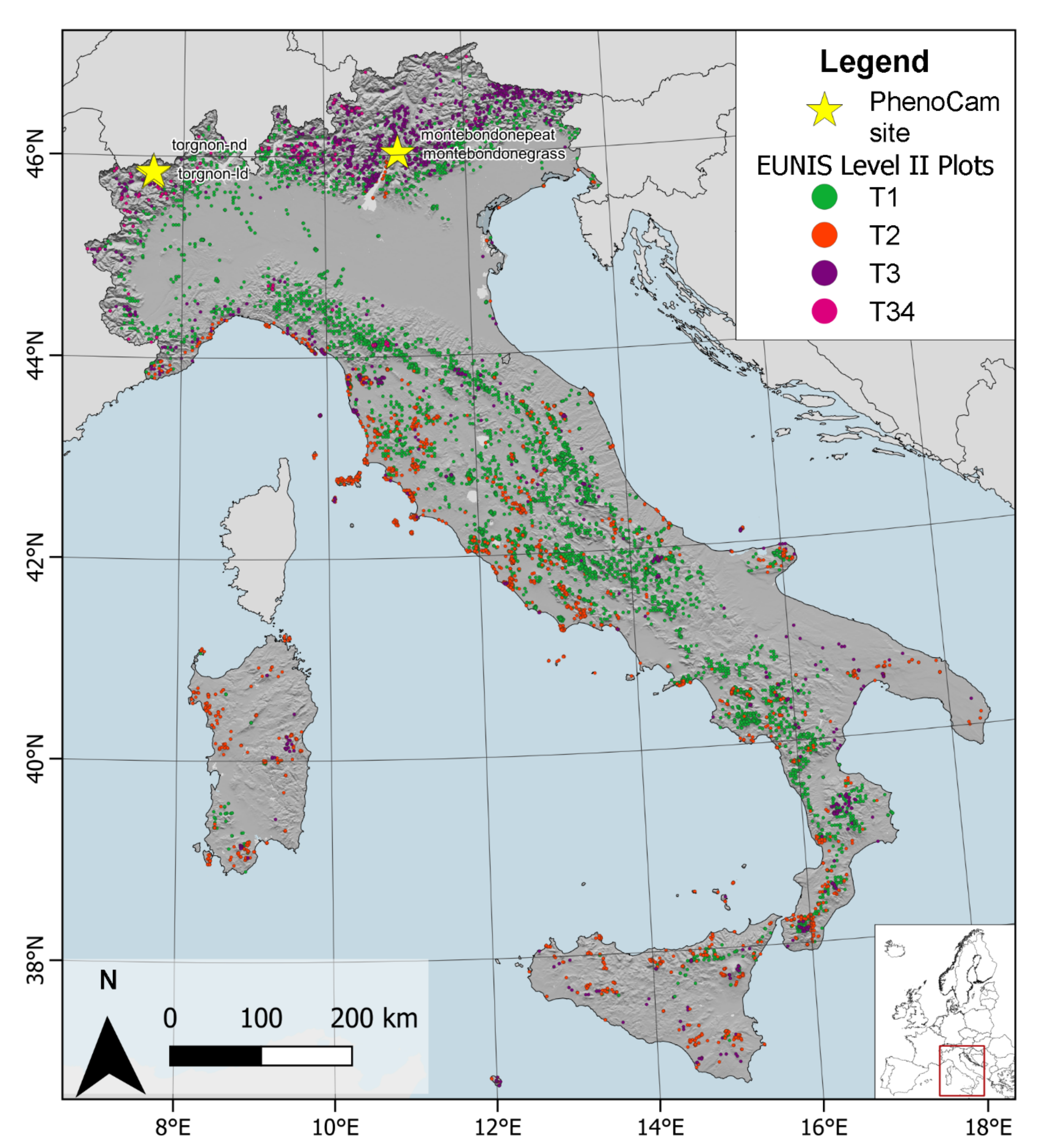
Figure 1. Overview of the study area showing location of PhenoCam sites used for validation and the spatial distribution of forest types plots classified using EUNIS level II classification (T1: broadleaved deciduous forest; T2: broadleaved evergreen forest; T3: needleleaved evergreen forest and, T34: needleleaved deciduous forest). PhenoCam data source: https://phenocam.sr.unh.edu/webcam (accessed on 11 March 2021).
Remotesensing 14 00721 g001
Figure 2. Flowchart of the main phases of the procedure to generate phenological metrics datasets and to perform multivariate statistical analysis. White ellipse refers to input data, grey boxes refer to data processing phases, black ellipses refer to output products.
Remotesensing 14 00721 g002
Figure 3. Smoothed LAI time series with estimated phenological metrics.
Remotesensing 14 00721 g003
Figure 4. Maps of selected phenological metrics estimated for the study area (year 2019). (a) LAI winter minimum; (b) LAI average; (c) Largest Greenup rate; (d) End of Growing Season date.
Remotesensing 14 00721 g004
Figure 5. Phenological metrics dates (expressed as DoY) derived from the GCC90 time series on the x-axis plotted against the estimates from S2 LAI on the y-axis. The dashed black line shows the 1:1 relationship.
Remotesensing 14 00721 g005
Figure 6. Biplots showing results of multivariate analysis. (a) Distribution of centers of gravity (black squares) for the EUNIS level II forest classes and LAI daily time series daily (colored dots) according to the first two DFA factors; (b) distribution of centers of gravity (black squares) for the EUNIS level III forest classes and LAI daily time series (colored dots) according to the first two DFA factors; (c) distribution of centers of gravity (black squares) for the EUNIS level II forest classes and LAI temporal statistics (colored dots) according to the first two DFA factors; (d) distribution of centers of gravity (black squares) for the EUNIS level III forest classes and LAI temporal statistics (red dots) according to the first two DFA factors; (e) distribution of centers of gravity (black squares) for the deciduous broadleaved (T1) forest classes and the sets of independent axes derived from CCA (red dots) according to the first two LDA factors; (f) distribution of centers of gravity (black squares) for the deciduous broadleaved (T1) forest classes and the sets of independent axes derived from CCA (red dots) according to the first and the third LDA factors.
Remotesensing 14 00721 g006
Table 1. Forest types selected according to EUNIS II and III level classification nomenclature.
EUNIS Code Level IIEUNIS Code Level IIIDescriptionPlots
T1 Broadleaved deciduous forest habitat8328
T11Temperate Salix and Populus riparian forest1027
T15Broadleaved swamp forest on non-acid peat772
T17Fagus forest on non-acid soils2404
T18Fagus forest on acid soils614
T19Temperate and sub-Mediterranean thermophilous deciduous forest1389
T1AMediterranean thermophilous deciduous forest815
T1BAcidophilous Quercus forest147
T1CTemperate and boreal mountain Betula and P. tremula forest on mineral soils32
T1DSouthern European mountain Betula and P. tremula forest on mineral soils36
T1ECarpinus and Quercus mesic deciduous forest260
T1FRavine forest541
T1GA. cordata forest291
T2 Broadleaved evergreen forest habitat3776
T3 Needleleaved evergreen forest habitat2281
T34 * Needleleaved deciduous forest habitat
Temperate subalpine Larix, P. cembra and P. uncinata forest
461
* This class has been examined separately from T3 EUNIS level II class since it belongs to needleleaved deciduous plant functional type.
Table 2. List and description of the estimated phenological metrics used. Time field reports the units used for the estimation (x-axis in Figure 2); Value field specify if vegetation index is computed for the corresponding phenological metric (y axis in Figure 2). DoY: day of year, VI: vegetation index.
Phenological metricTimeValueAcronymDescription
Start of Seasondate, DoYVISoSMinimum VI value before the onset of photosynthesis
Start of Growing Seasondate, DoYVISGSBeginning of measurable photosynthesis in the vegetation canopy
greenup VI rategreenupMaximum positive slope of the curve during the onset of photosynthesis
Peak of Seasondate, DoYVIPoSMaximum level of photosynthetic activity in the canopy during the growing season
End of Growing Seasondate, DoYVIEGSBeginning of significant degradation of chlorophyll revealing various accessory pigments
senescence VI ratesenescenceMaximum negative slope of the curve during the chlorophyll degradation
End of Seasondate, DoYVIEoSEnd of measurable photosynthesis in the vegetation canopy
Amplitude VIAmpMaximum increase in canopy photosynthetic activity above the baseline
Plateau slope VI rateplateau_slopeSlope during the maturity phase
Duration of Seasondays DoSLength of photosynthetic activity during the growing season
Length of Maturity Plateaudays LMPLength of photosynthetic activity during the maturity phase
Seasonal Time Integrated index VISTICanopy photosynthetic activity across the entire growing season calculated as daily integration of VI values
Table 3. PhenoCam network sites.
Site NameEcosystem TypeLongitudeLatitudeElevation
torgnon-ldDeciduous Needleaved Forest7.560945.82382091
torgnon-ndGrassland7.578145.84442160
montebondonegrassGrassland11.045846.01471550
montebondonepeatPeatland11.040946.01771563
Table 4. Accuracy assessment results for the comparison of phenological metrics estimated from ground PhenoCam GCC90 time series and S2 LAI time series. ME: Mean Error, MAE: Mean Absolute Error, RMSE: Root Mean Square Error, r: correlation coefficient. SGS: Start of Growing Season, PoS: Peak of Season, EGS: End of Growing Season, EoS: End of Season.
MEMAERMSEr
SGS6.3514.4717.710.6758
PoS−26.9426.9427.560.8804
EGS−1.1814.5918.060.8555
EoS−13.4114.8220.50.7645
greenup−317.9422.190.4079
senescence−8.5918.4724.040.6242
Publisher’s Note: MDPI stays neutral with regard to jurisdictional claims in published maps and institutional affiliations.