
Earth Observation for Phenological Metrics (EO4PM): Temporal Discriminant to Characterize Forest Ecosystems


Abstract
:1. Introduction
2. Materials and Methods
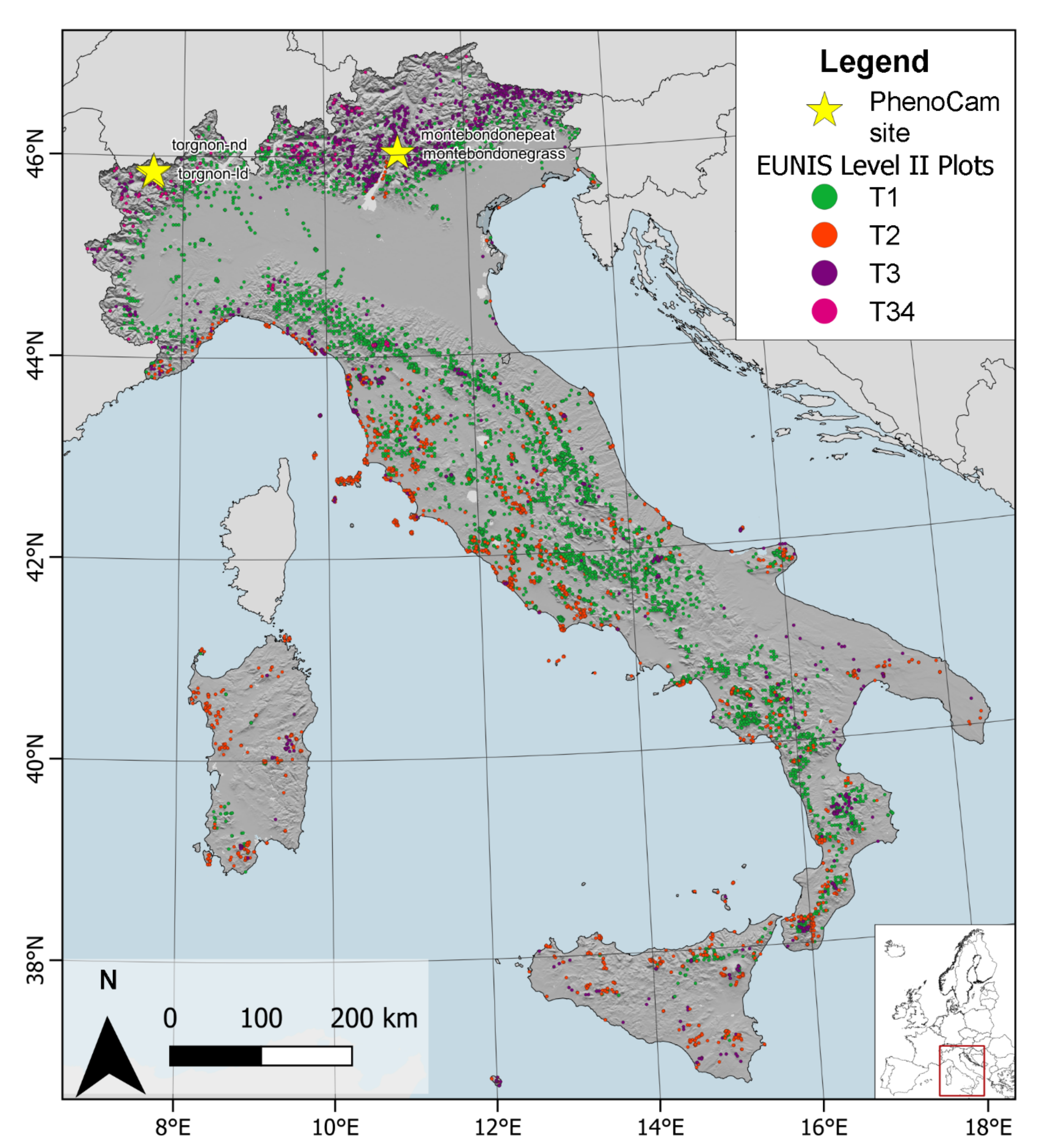
2.1. Study Area
2.2. Forest Habitat Types
2.3. Satellite Data
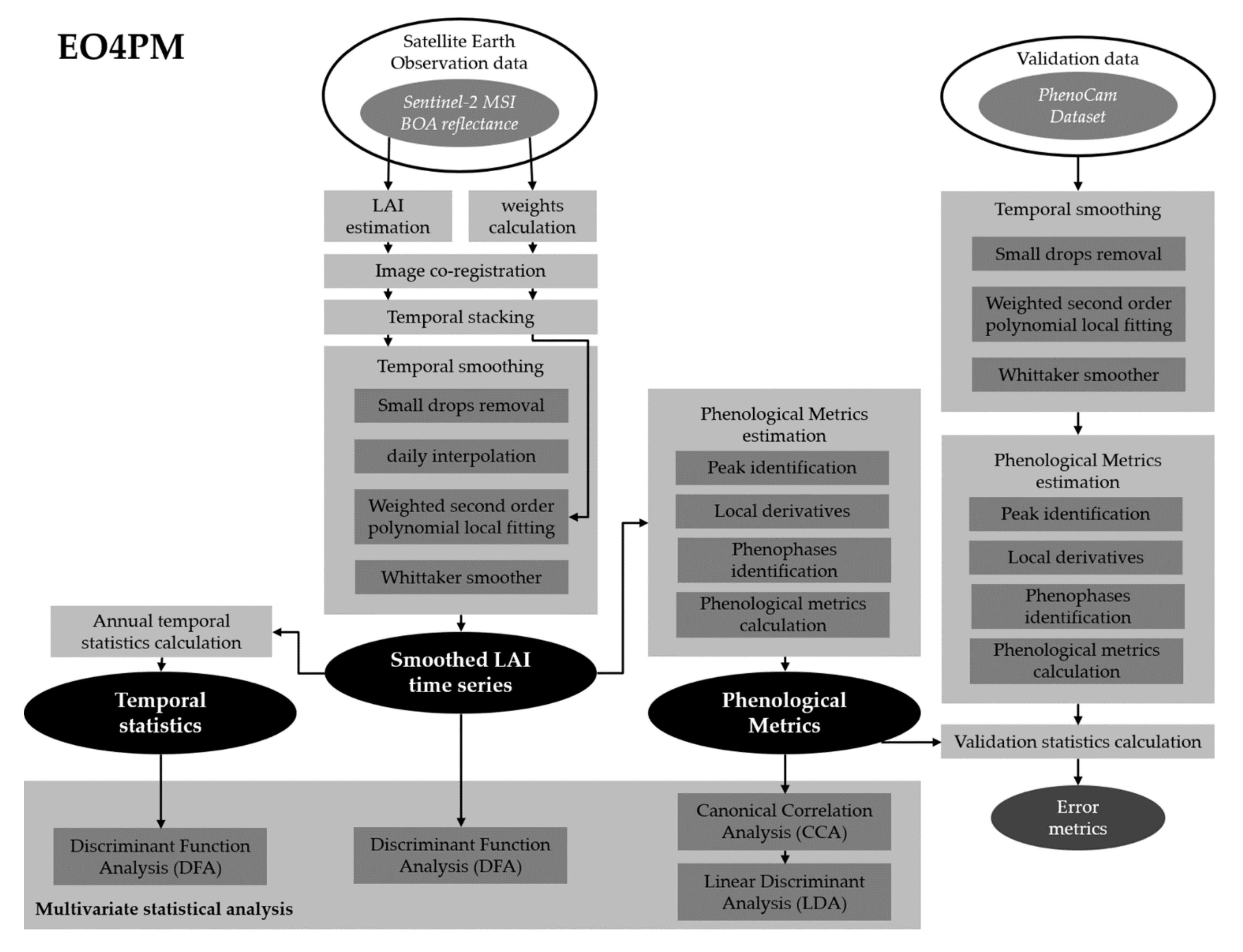
2.4. Satellite Data Processing
2.5. Phenological Metrics Accuracy Assessment
2.6. Multivariate Analysis
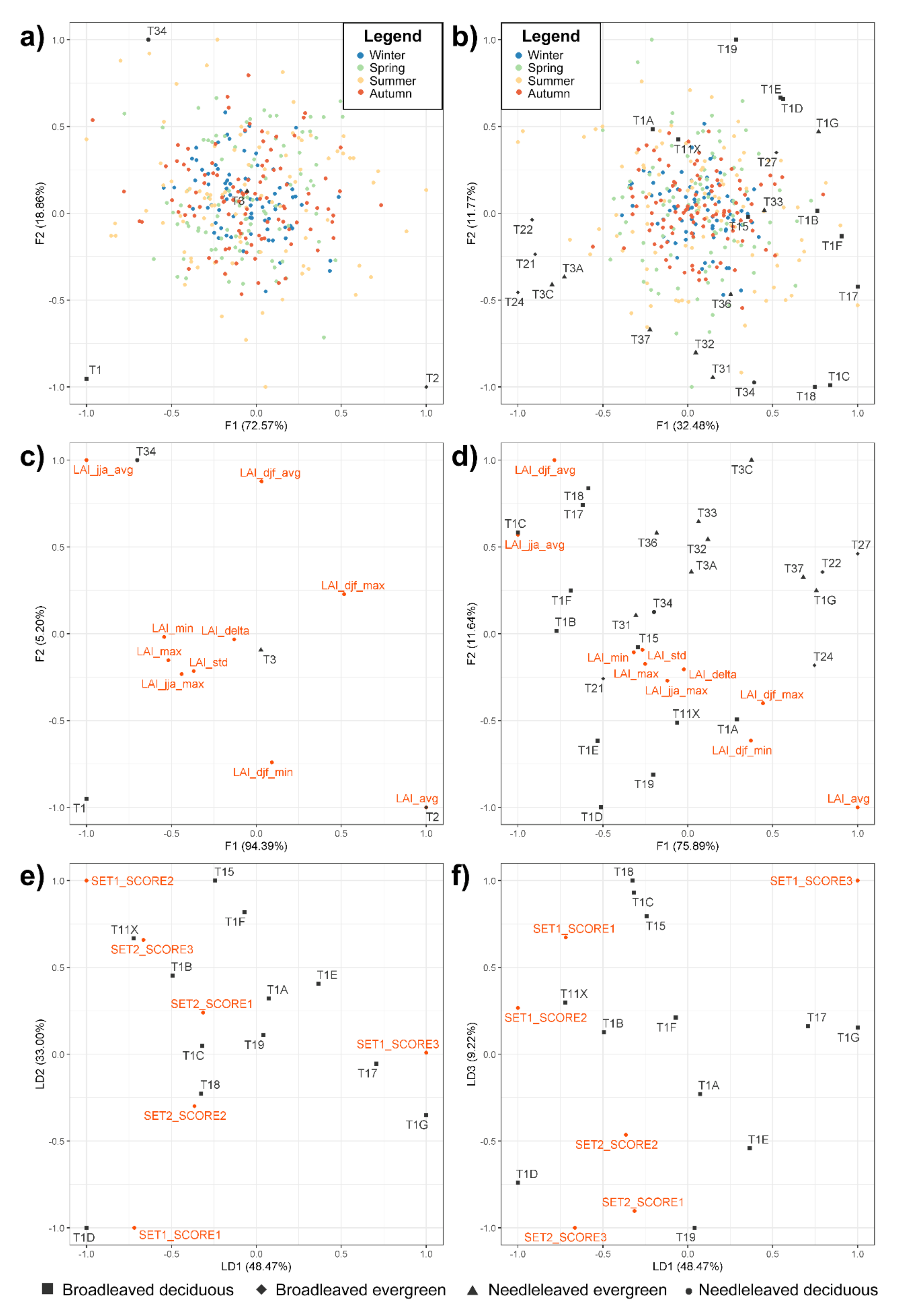
- Regarding the smoothed vegetation curve and the temporal statistics variables (predictors), a DFA was executed to identify the variables able to discriminate the forest types (response variables) at the EUNIS II level;
- As for the phenological metrics, a two steps analysis was performed for T1 EUNIS III level classes. Since the presence of two sets of variables, firstly a CCA was run on the phenological metrics dataset illustrated in Table 2 and constituted of 10 variables of LAI values and 9 variables of date values. The resulting independent and representative axes were then used to perform a LDA to discriminate the deciduous broadleaved forest types.
3. Results
4. Discussion
5. Conclusions
Author Contributions
Funding
Institutional Review Board Statement
Informed Consent Statement
Acknowledgments
Conflicts of Interest
Appendix A
References
- Betancourt, J.L.; Schwartz, M.D.; Breshears, D.D.; Brewer, C.A.; Frazer, G.; Gross, J.E.; Mazer, S.J.; Reed, B.C.; Wilson, B.E. Evolving plans for the USA National Phenology Network. Eos Trans. AGU 2007, 88, 211. [Google Scholar] [CrossRef]
- Van Vliet, A.J.H.; de Groot, R.S.; Bellens, Y.; Braun, P.; Bruegger, R.; Bruns, E.; Clevers, J.; Estreguil, C.; Flechsig, M.; Jeanneret, F.; et al. The European Phenology Network. Int. J. Biometeorol. 2003, 47, 202–212. [Google Scholar] [CrossRef] [PubMed]
- Nasahara, K.N.; Nagai, S. Review: Development of an in situ observation network for terrestrial ecological remote sensing: The Phenological Eyes Network (PEN). Ecol. Res. 2015, 30, 211–223. [Google Scholar] [CrossRef]
- Templ, B.; Koch, E.; Bolmgren, K.; Ungersböck, M.; Paul, A.; Scheifinger, H.; Busto, M.; Chmielewski, F.M.; Hájková, L.; Hodzic, S. Pan European Phenological database (PEP725): A single point of access for European data. Int. J. Biometeorol. 2018, 62, 1109–1113. [Google Scholar] [CrossRef]
- Lieth, H. Phenology and Seasonality Modeling; Springer: Berlin/Heidelberg, Germany, 1974. [Google Scholar]
- Baddour, O.; Kontongomde, H. Guidelines for Plant Phenological Observations; WMO-TD No. 1484; World Meteorological Organization: Geneva, Switzerland, 2009. [Google Scholar]
- Schwartz, M.D. Phenology: An Integrative Environmental Science; Springer: Dordrecht, The Netherlands, 2013. [Google Scholar]
- IPCC (Intergovernmental Panel on Climate Change). Climate Change 2001: The Scientific Basis. Contribution of Working Group I to the Third Assessment Report of the Intergovernmental Panel on Climate Change; Houghton, J.T., Ding, Y., Griggs, D.J., Noguer, M., van der Linden, P.J., Dai, X., Maskell, K., Johnson, C.A., Eds.; Cambridge University Press: New York, NY, USA, 2001. [Google Scholar]
- Myneni, R.B.; Keeling, C.D.; Tucker, C.J.; Asrar, G.; Nemani, R.R. Increased plant growth in the northern high latitudes from 1981 to 1991. Nature 1997, 386, 698–702. [Google Scholar] [CrossRef]
- Walkovszky, A. Changes in phenology of the locust tree (Robinia pseudoacacia L) in Hungary. Int. J. Biometeorol. 1998, 41, 155–160. [Google Scholar] [CrossRef]
- Chmielewski, F.M.; Roetzer, T. Phenological trends in Europe in relation to climatic changes. Agrarmeteorol. Schr. 2000, 7, 1–15. [Google Scholar]
- Schwartz, M.D.; Reiter, B.E. Changes in North American spring. Int. J. Climatol. 2000, 20, 929–932. [Google Scholar] [CrossRef]
- Menzel, A.; Estrella, N.; Fabian, P. Spatial and temporal variability of the phenological seasons in Germany from 1951–1996. Global Change Biol. 2001, 7, 657–666. [Google Scholar] [CrossRef]
- Brown, M.E.; de Beurs, K.M. The response of African land surface phenology to large scale climate oscillations. Remote Sens. Environ. 2010, 10, 2286–2296. [Google Scholar] [CrossRef] [Green Version]
- Menzel, A.; Seifert, H.; Estrella, N. Effects of recent warm and cold spells on European plant phenology. Int. J. Biometeorol. 2011, 55, 921–932. [Google Scholar] [CrossRef]
- Noormets, A. Phenology of Ecosystem Processes; Springer: New York, NY, USA, 2009. [Google Scholar]
- Visser, M.E.; Caro, S.P.; van Oers, K.; Schaper, S.V.; Helm, B. Phenology, seasonal timing and circannual rhythms: Towards a unified framework. Philosoph. Trans. R. Soc. B—Biol. Sci. 2010, 365, 3113–3127. [Google Scholar] [CrossRef] [PubMed] [Green Version]
- Menzel, A.; Sparks, T.; Estrella, N.; Koch, E.; Aasa, A.; Ahas, R.; Alm-Kübler, K.; Bissolli, P.; Braslavská, O.; Briede, A.; et al. European phenological response to climate change matches the warming pattern. Glob. Change Biol. 2006, 12, 1969–1976. [Google Scholar] [CrossRef]
- Menzel, A.; Dose, V. Analysis of long-term time-series of beginning of flowering by Bayesian function estimation. Meteorologische Zeitschrift 2005, 14, 429–434. [Google Scholar] [CrossRef] [Green Version]
- Meier, U.; Bleiholder, H.; Buhr, L.; Feller, C.; Hack, H.; Hess, M.; Lancashire, P.D.; Schnock, U.; Stauss, R.; van den Boom, T.; et al. The BBCH system to coding the phenological growth stages of plants—History and publications. J. für Kulturpflanzen 2009, 61, 41–52. [Google Scholar] [CrossRef]
- Morisette, J.T.; Richardson, A.D.; Knapp, A.K.; Fisher, J.I.; Graham, E.A.; Abatzoglou, J.; Wilson, B.E.; Breshears, D.D.; Henebry, G.M.; Hanes, J.M.; et al. Tracking the rhythm of the seasons in the face of global change: Phenological research in the 21st Century. Front. Ecol. Environ. 2009, 7, 253–260. [Google Scholar] [CrossRef] [Green Version]
- Filippa, G.; Cremonese, E.; Migliavacca, M.; Galvagno, M.; Forkel, M.; Wingate, L.; Tomelleri, E.; Morra di Cella, U.; Richardson, A.D. Phenopix: AR package for image-based vegetation phenology. Agric. For. Meteorol. 2016, 220, 141–150. [Google Scholar] [CrossRef] [Green Version]
- Bajocco, S.; Raparelli, E.; Teofili, T.; Bascietto, M.; Ricotta, C. Text Mining in Remotely Sensed Phenology Studies: A Review on Research Development, Main Topics, and Emerging Issues. Remote Sens. 2019, 11, 2751. [Google Scholar] [CrossRef] [Green Version]
- Jeong, S.J.; Ho, C.H.; Gim, H.J.; Brown, M.E. Phenology shifts at start vs. end of growing season in temperate vegetation over the Northern Hemisphere for the period 1982–2008. Glob. Change Biol. 2011, 17, 2385–2399. [Google Scholar] [CrossRef]
- Zeng, L.; Wardlow, B.; Xiang, D.; Hu, S.; Li, D. A review of vegetation phenological metrics extraction using time-series, multispectral satellite data. Remote Sens. Environ. 2020, 237, 111511. [Google Scholar] [CrossRef]
- USA-NPN National Phenology Network. Land Surface Phenology and Remote Sensing (LSP/RS). Available online: https://usanpn.org/node/14 (accessed on 21 November 2021).
- De Beurs, K.M.; Henebry, G.M. Land surface phenology and temperature variation in the International Geosphere–Biosphere Program high-latitude transects. Glob. Change Biol. 2005, 11, 779–790. [Google Scholar] [CrossRef]
- Roy, D.P.; Lewis, P.; Schaaf, C.; Devadiga, S.; Boschetti, L. The global impact of cloud on the production of MODIS bi-directional reflectance model based composites for terrestrial monitoring. IEEE Geosci. Remote Sens. Lett. 2006, 3, 452–456. [Google Scholar] [CrossRef] [Green Version]
- Duchemin, B.; Goubier, J.; Courrier, G. Monitoring phenological key stages and cycle duration of temperate deciduous forest ecosystems with NOAA/AVHRR data. Remote Sens. Environ. 1999, 67, 68–82. [Google Scholar] [CrossRef]
- Heumann, B.W.; Seaquist, J.W.; Eklundh, L.; Jönsson, P. AVHRR derived phenological change in the Sahel and Soudan, Africa, 1982–2005. Remote Sens. Environ. 2007, 108, 385–392. [Google Scholar] [CrossRef]
- Zhang, X.; Friedl, M.A.; Schaaf, C.B.; Strahler, A.H.; Hodges, J.C.F.; Gao, F.; Reed, B.C.; Huete, A. Monitoring vegetation phenology using MODIS. Remote Sens. Environ. 2003, 84, 471–475. [Google Scholar] [CrossRef]
- Tan, B.; Morisette, J.T.; Wolfe, R.E.; Gao, F.; Ederer, G.A.; Nightingale, J.; Pedelty, J.A. An enhanced TIMESAT algorithm for estimating vegetation phenology metrics from MODIS data. IEEE J. Sel. Top. Appl. Earth Observ. Remote Sens. 2010, 4, 361–371. [Google Scholar] [CrossRef]
- Li, J.; Roy, D.P. A Global Analysis of Sentinel-2A, Sentinel-2B and Landsat-8 Data Revisit Intervals and Implications for Terrestrial Monitoring. Remote Sens. 2017, 9, 902. [Google Scholar] [CrossRef] [Green Version]
- Vrieling, A.; Meroni, M.; Darvishzadeh, R.; Skidmore, A.K.; Wang, T.; Zurita-Milla, R.; Oosterbeek, K.; O’Connor, B.; Paganini, M. Vegetation phenology from Sentinel-2 and field cameras for a Dutch barrier island. Remote Sens. Environ. 2018, 215, 517–529. [Google Scholar] [CrossRef]
- Kang, S.; Running, S.W.; Lim, J.H.; Zhao, M.; Park, C.R.; Loehman, R. A regional phenology model for detecting onset of greenness in temperate mixed forests, Korea: An application of MODIS leaf area index. Remote Sens. Environ. 2003, 86, 232–242. [Google Scholar] [CrossRef]
- Verhegghen, A.; Bontemps, S.; Defourny, P. A global NDVI and EVI reference data set for land-surface phenology using 13 years of daily SPOT-VEGETATION observations. Int. J. Remote Sens. 2014, 35, 2440–2471. [Google Scholar] [CrossRef] [Green Version]
- Wu, C.; Peng, D.; Soudani, K.; Siebicke, L.; Gough, C.M.; Arain, M.A.; Bohrer, G.; Lafleur, P.M.; Peichl, M.; Gonsamo, A. Land surface phenology derived from normalized difference vegetation index (NDVI) at global FLUXNET sites. Agric. For. Meteorol. 2017, 233, 171–182. [Google Scholar] [CrossRef]
- White, M.A.; Hoffman, F.M.; Hargrove, W.W.; Nemani, R.R. A global framework for monitoring phenological responses to climate change. Geophys. Res. Lett. 2005, 32, L04705. [Google Scholar] [CrossRef] [Green Version]
- Hargrove, W.W.; Spruce, J.P.; Gasser, G.E.; Hoffman, F.M. Toward a national early warning system for forest disturbances using remotely sensed canopy phenology. Photogramm. Eng. Remote Sens. 2009, 75, 1150–1156. [Google Scholar]
- Boschetti, M.; Nelson, A.; Nutini, F.; Manfron, G.; Busetto, L.; Barbieri, M.; Laborte, A.; Raviz, J.; Holecz, F.; Mabalay, M.R.O.; et al. Rapid Assessment of Crop Status: An Application of MODIS and SAR Data to Rice Areas in Leyte, Philippines Affected by Typhoon Haiyan. Remote Sens. 2015, 7, 6535–6557. [Google Scholar] [CrossRef] [Green Version]
- Bajocco, S.; Ferrara, C.; Alivernini, A.; Bascietto, M.; Ricotta, C. Remotely-sensed phenology of Italian forests: Going beyond the species. Int. J. Appl. Earth Obs. Geoinf. 2019, 74, 314–321. [Google Scholar] [CrossRef]
- Pesaresi, S.; Mancini, A.; Casavecchia, S. Recognition and Characterization of Forest Plant Communities through Remote-Sensing NDVI Time Series. Diversity 2020, 12, 313. [Google Scholar] [CrossRef]
- Valero, S.; Morin, D.; Inglada, J.; Sepulcre, G.; Arias, M.; Hagolle, O.; Dedieu, G.; Bontemps, S.; Defourny, P.; Koetz, B. Production of a Dynamic Cropland Mask by Processing Remote Sensing Image Series at High Temporal and Spatial Resolutions. Remote Sens. 2016, 8, 55. [Google Scholar] [CrossRef] [Green Version]
- Boschetti, M.; Busetto, L.; Manfron, G.; Laborte, A.; Asilo, S.; Pazhanivelan, S.; Nelson, A. PhenoRice: A method for automatic extraction of spatio-temporal information on rice crops using satellite data time series. Remote Sens. Environ. 2017, 194, 347–365. [Google Scholar] [CrossRef] [Green Version]
- Reed, B.C.; Brown, J.F.; VanderZee, D.; Loveland, T.R.; Merchant, J.W.; Ohlen, D.O. Measuring phenological variability from satellite data. J. Veg. Sci. 1994, 5, 703–714. [Google Scholar] [CrossRef]
- Gu, Y.; Brown, J.F.; Miura, T.; van Leeuwen, W.J.D.; Reed, B.C. Phenological Classification of the United States: A Geographic Framework for Extending Multi-Sensor Time-Series Data. Remote Sens. 2010, 2, 526–544. [Google Scholar] [CrossRef] [Green Version]
- Clerici, N.; Weissteiner, C.J.; Gerard, F. Exploring the Use of MODIS NDVI-Based Phenology Indicators for Classifying Forest General Habitat Categories. Remote Sens. 2012, 4, 1781–1803. [Google Scholar] [CrossRef] [Green Version]
- White, M.A.; Thornton, P.E.; Running, S.W. A continental phenology model for monitoring vegetation responses to interannual climatic variability. Glob. Biogeochem. Cycles 1997, 11, 217–234. [Google Scholar] [CrossRef]
- Curnel, Y.; Oger, R. Agrophenology Indicators from Remote Sensing: State of the Art. Available online: https://www.isprs.org/proceedings/XXXVI/8-W48/ (accessed on 22 December 2021).
- De Beurs, K.M.; Henebry, G.M. Spatio-Temporal Statistical Methods for Modeling Land Surface Phenology. In Phenological Research: Methods for Environmental and Climate Change Analysis; Hudson, I.L., Keatley, M.R., Eds.; Springer: Dordrecht, The Netherlands, 2010; pp. 177–208. [Google Scholar] [CrossRef]
- Xu, H.; Twine, T.E.; Yang, X. Evaluating Remotely Sensed Phenological Metrics in a Dynamic Ecosystem Model. Remote Sens. 2014, 6, 4660–4686. [Google Scholar] [CrossRef] [Green Version]
- Matongera, T.N.; Mutanga, O.; Sibanda, M.; Odindi, J. Estimating and Monitoring Land Surface Phenology in Rangelands: A Review of Progress and Challenges. Remote Sens. 2021, 13, 2060. [Google Scholar] [CrossRef]
- European Environment Agency (EEA). High Resolution Vegetation Phenology and Productivity (HR-VPP), Seasonal Trajectories and VPP parameters; Copernicus Land Monitoring Service, European Environment Agency: Copenhagen, Denmark, 2021. [Google Scholar]
- High Resolution Vegetation Phenology and Productivity. Available online: https://land.copernicus.eu/pan-european/biophysical-parameters/high-resolution-vegetation-phenology-and-productivity (accessed on 22 December 2021).
- Tian, F.; Cai, Z.; Jin, H.; Hufkens, K.; Scheifinger, H.; Tagesson, T.; Smets, B.; Van Hoolst, R.; Bonte, K.; Ivits, E.; et al. Calibrating vegetation phenology from Sentinel-2 using eddy covariance, PhenoCam, and PEP725 networks across Europe. Remote Sens. Environ. 2021, 260, 112456. [Google Scholar] [CrossRef]
- Pesaresi, S.; Galdenzi, D.; Biondi, E.; Casavecchia, S. Bioclimate of Italy: Application of the worldwide bioclimatic classification system. J. Maps 2014, 10, 538–553. [Google Scholar] [CrossRef]
- Copertura del Suolo. Available online: https://www.isprambiente.gov.it/it/attivita/suolo-e-territorio/copertura-del-suolo (accessed on 22 December 2021).
- Chytrý, M.; Hennekens, S.M.; Jiménez-Alfaro, B.; Knollová, I.; Dengler, J.; Jansen, F.; Landucci, F.; Schaminée, J.H.; Acìc, S.; Agrillo, E.; et al. European Vegetation Archive (EVA): An integrated database of European vegetation plots. Appl. Veg. Sci. 2016, 19, 173–180. [Google Scholar] [CrossRef] [Green Version]
- Agrillo, E.; Alessi, N.; Massimi, M.; Spada, F.; De Sanctis, M.; Francesconi, F.; Cambria, V.E.; Attorre, F. Nationwide Vegetation Plot Database-Sapienza University of Rome: State of the art, basic figures and future perspectives. Phytocoenologia 2017, 47, 221–222. [Google Scholar] [CrossRef]
- Chytrý, M.; Tichý, L.; Hennekens, S.M.; Knollová, I.; Janssen, J.A.; Rodwell, J.S.; Peterka, T.; Marcenò, C.; Landucci, F.; Dani-helka, J.; et al. EUNIS Habitat Classification: Expert system, characteristic species combinations and distribution maps of European habitats. Appl. Veg. Sci. 2020, 23, 648–675. [Google Scholar] [CrossRef]
- Agrillo, E.; Filipponi, F.; Pezzarossa, A.; Casella, L.; Smiraglia, D.; Orasi, A.; Attorre, F.; Taramelli, A. Earth Observation and Biodiversity Big Data for Forest Habitat Types Classification and Mapping. Remote Sens. 2021, 13, 1231. [Google Scholar] [CrossRef]
- Löw, M.; Koukal, T. Phenology Modelling and Forest Disturbance Mapping with Sentinel-2 Time Series in Austria. Remote Sens. 2020, 12, 4191. [Google Scholar] [CrossRef]
- Hagolle, O.; Huc, M.; Desjardins, C.; Auer, S.; Richter, R. MAJA Algorithm Theoretical Basis Document; CNES: Paris, France, 2017. [Google Scholar] [CrossRef]
- Rouquié, B.; Hagolle, O.; Bréon, F.M.; Boucher, O.; Desjardins, C.; Rémy, S. Using Copernicus atmosphere monitoring service products to constrain the aerosol type in the atmospheric correction processor MAJA. Remote Sens. 2017, 9, 1230. [Google Scholar] [CrossRef] [Green Version]
- Weiss, M.; Baret, F. S2 ToolBox Level 2 Products: LAI, FAPAR, FCOVER. 2016. Available online: https://step.esa.int/docs/extra/ATBD_S2ToolBox_L2B_V1.1.pdf (accessed on 21 November 2021).
- Djamai, N.; Fernandes, R.; Weiss, M.; McNairn, H.; Goïta, K. Validation of the Sentinel Simplified Level 2 Product Prototype Processor (SL2P) for mapping cropland biophysical variables using Sentinel-2/MSI and Landsat-8/OLI data. Remote Sens. Environ. 2019, 225, 416–430. [Google Scholar] [CrossRef]
- Scheffler, D.; Hollstein, A.; Diedrich, H.; Segl, K.; Hostert, P. AROSICS: An Automated and Robust Open-Source Image Co-Registration Software for Multi-Sensor Satellite Data. Remote Sens. 2017, 9, 676. [Google Scholar] [CrossRef] [Green Version]
- Filipponi, F. Exploitation of Sentinel-2 Time Series to Map Burned Areas at the National Level: A Case Study on the 2017 Italy Wildfires. Remote Sens. 2019, 11, 622. [Google Scholar] [CrossRef] [Green Version]
- Manfron, G.; Crema, A.; Boschetti, M.; Confalonieri, R. Testing Automatic Procedures to Map Rice Area and Detect Phenological Crop Information Exploiting Time Series Analysis of Remote Sensed MODIS Data. In Remote Sensing for Agriculture, Ecosystems, and Hydrology XIV, Proceedings of the SPIE 8531, Edinburgh, UK, 24–26 September 2012; Society of Photo-Optical Instrumentation Engineers (SPIE): Bellingham, WA, USA, 2012; Volume 8531, p. 85311E. [Google Scholar] [CrossRef]
- Johannesson, T.; Bjornsson, H. Stinepack: Stineman, a Consistently Well Behaved Method of Interpolation. R Package Version 1.3. 2012. Available online: https://CRAN.R-project.org/package=stinepack (accessed on 21 November 2021).
- Stineman, R.W. A Consistently Well Behaved Method of Interpolation. Creat. Comput. 1980, 6, 54–57. [Google Scholar]
- Chen, J.; Jönsson, P.; Tamura, M.; Gu, Z.; Matsushita, B.; Eklundh, L. A simple method for reconstructing a high-quality NDVI time-series data set based on the Savitzky-Golay filter. Remote Sens. Environ. 2004, 91, 332–344. [Google Scholar] [CrossRef]
- Whittaker, E.T. On a new method of graduation. Proc. Edinb. Math. Soc. 1923, 41, 63–75. [Google Scholar] [CrossRef] [Green Version]
- Eilers, P.H. A perfect smoother. Anal. Chem. 2003, 75, 3631–3636. [Google Scholar] [CrossRef]
- Bloemberg, T.G.; Gerretzen, J.; Wouters, H.J.; Gloerich, J.; van Dael, M.; Wessels, H.J.; van den Heuvel, L.P.; Eilers, P.H.C.; Buydens, L.M.C.; Wehrens, R. Improved parametric time warping for proteomics. Chemom. Intell. Lab. Syst. 2010, 104, 65–74. [Google Scholar] [CrossRef]
- Gu, L.; Post, W.M.; Baldocchi, D.D.; Black, T.A.; Suyker, A.E.; Verma, S.B.; Vesala, T.; Wofsy, S.C. Characterizing the Seasonal Dynamics of Plant Community Photosynthesis Across a Range of Vegetation Types. In Phenology of Ecosystem Processes; Noormets, A., Ed.; Springer: Berlin/Heidelberg, Germany, 2009; pp. 35–58. [Google Scholar] [CrossRef] [Green Version]
- Huang, X.; Liu, J.; Zhu, W.; Atzberger, C.; Liu, Q. The Optimal Threshold and Vegetation Index Time Series for Retrieving Crop Phenology Based on a Modified Dynamic Threshold Method. Remote Sens. 2019, 11, 2725. [Google Scholar] [CrossRef] [Green Version]
- Richardson, A.D.; Hufkens, K.; Milliman, T.; Aubrecht, D.M.; Chen, M.; Gray, J.M.; Johnston, M.R.; Keenan, T.F.; Klosterman, S.T.; Kosmala, M.; et al. Tracking vegetation phenology across diverse North American biomes using PhenoCam imagery. Sci. Data 2018, 5, 180028. [Google Scholar] [CrossRef] [PubMed]
- Seyednasrollah, B.; Young, A.M.; Hufkens, K.; Milliman, T.; Friedl, M.A.; Frolking, S.; Richardson, A.D. Tracking vegetation phenology across diverse biomes using version 2.0 of the phenocam dataset. Sci. Data 2019, 6, 222. [Google Scholar] [CrossRef] [PubMed] [Green Version]
- Huberty, C.J.; Olejnik, S. Applied MANOVA and Discriminant Analysis, 2nd ed.; Wiley: Hoboken, NJ, USA, 2006; ISBN 978-0-471-46815-8. [Google Scholar]
- Gittins, R. Canonical Analysis. A Review with Application in Ecology; Springer: Berlin/Heidelberg, Germany, 1985. [Google Scholar]
- Fisher, R.A. The Use of Multiple Measurements in Taxonomic Problems. Ann. Eugen. 1936, 7, 179–188. [Google Scholar] [CrossRef]
- Badgley, G.; Field, C.; Berry, J. Canopy near-infrared reflectance and terrestrial photosynthesis. Sci. Adv. 2017, 3, e1602244. [Google Scholar] [CrossRef] [Green Version]
- Camps-Valls, G.; Campos-Taberner, M.; Moreno-Martínez, Á.; Walther, S.; Duveiller, G.; Cescatti, A.; Mahecha, M.D.; Muñoz-Marí, J.; García-Haro, F.J.; Guanter, L.; et al. A unified vegetation index for quantifying the terrestrial biosphere. Sci. Adv. 2021, 7, eabc7447. [Google Scholar] [CrossRef]
- Earth Resources Observation and Science (EROS) Center. USGS EROS Archive-Vegetation Monitoring-eMODIS Remote Sensing Phenology. 2018. Available online: https://www.usgs.gov/centers/eros/science/usgs-eros-archive-vegetation-monitoring-emodis-remote-sensing-phenology (accessed on 22 December 2021).
- Jönsson, P.; Eklundh, L. TIMESAT-a program for analyzing time-series of satellite sensor data. Comput. Geosci. 2004, 30, 833–845. [Google Scholar] [CrossRef] [Green Version]
- Baetens, L.; Desjardins, C.; Hagolle, O. Validation of Copernicus Sentinel-2 Cloud Masks Obtained from MAJA, Sen2Cor, and FMask Processors Using Reference Cloud Masks Generated with a Supervised Active Learning Procedure. Remote Sens. 2019, 11, 433. [Google Scholar] [CrossRef] [Green Version]
- Vrieling, A.; Skidmore, A.K.; Wang, T.; Meroni, M.; Ens, B.J.; Oosterbeek, K.; O’Connor, B.; Darvishzadeh, R.; Heurich, M.; Shepherd, A.; et al. Spatially detailed retrievals of spring phenology from single-season high-resolution image time series. Int. J. Appl. Earth Obs. Geoinf. 2017, 59, 19–30. [Google Scholar] [CrossRef]
- White, K.; Pontius, J.; Schaberg, P. Remote sensing of spring phenology in northeastern forests: A comparison of methods, field metrics and sources of uncertainty. Remote Sens. Environ. 2014, 148, 97–107. [Google Scholar] [CrossRef]
- Liu, J.; Huang, X. Evaluating Crop Phenology Retrieving Accuracies Based on Ground Observations. In Proceedings of the 8th International Conference on Agro-Geoinformatics (Agro-Geoinformatics), Istanbul, Turkey, 16–19 July 2019; pp. 1–5. [Google Scholar] [CrossRef]
- Frantz, D. FORCE—Landsat + Sentinel-2 Analysis Ready Data and Beyond. Remote Sens. 2019, 11, 1124. [Google Scholar] [CrossRef] [Green Version]
- Kollert, A.; Bremer, M.; Löw, M.; Rutzinger, M. Exploring the Potential of Land Surface Phenology and Seasonal Cloud Free Composites of One Year of Sentinel-2 Imagery for Tree Species Mapping in a Mountainous Region. Int. J. Appl. Earth Obs. Geoinf. 2021, 94, 102208. [Google Scholar] [CrossRef]
- Kolecka, N.; Ginzler, C.; Pazur, R.; Price, B.; Verburg, P.H. Regional Scale Mapping of Grassland Mowing Frequency with Sentinel-2 Time Series. Remote Sens. 2018, 10, 1221. [Google Scholar] [CrossRef] [Green Version]
- Filipponi, F.; Smiraglia, D.; Mandrone, S.; Tornato, A. Cropland mapping using Earth Observation derived phenological metrics. Biol. Life Sci. Forum 2021. submitted for publication. [Google Scholar]
- Richardson, A.D.; Keenan, T.F.; Migliavacca, M.; Ryu, Y.; Sonnentag, O.; Toomey, M. Climate change, phenology, and phenological control of vegetation feedbacks to the climate system. Agric. For. Meteorol. 2013, 169, 156–173. [Google Scholar] [CrossRef]
- Rüetschi, M.; Schaepman, M.E.; Small, D. Using Multitemporal Sentinel-1 C-band Backscatter to Monitor Phenology and Classify Deciduous and Coniferous Forests in Northern Switzerland. Remote Sens. 2018, 10, 55. [Google Scholar] [CrossRef] [Green Version]
- Frison, P.-L.; Fruneau, B.; Kmiha, S.; Soudani, K.; Dufrêne, E.; Le Toan, T.; Koleck, T.; Villard, L.; Mougin, E.; Rudant, J.-P. Potential of Sentinel-1 Data for Monitoring Temperate Mixed Forest Phenology. Remote Sens. 2018, 10, 2049. [Google Scholar] [CrossRef] [Green Version]


| EUNIS Code Level II | EUNIS Code Level III | Description | Plots |
|---|---|---|---|
| T1 | Broadleaved deciduous forest habitat | 8328 | |
| T11 | Temperate Salix and Populus riparian forest | 1027 | |
| T15 | Broadleaved swamp forest on non-acid peat | 772 | |
| T17 | Fagus forest on non-acid soils | 2404 | |
| T18 | Fagus forest on acid soils | 614 | |
| T19 | Temperate and sub-Mediterranean thermophilous deciduous forest | 1389 | |
| T1A | Mediterranean thermophilous deciduous forest | 815 | |
| T1B | Acidophilous Quercus forest | 147 | |
| T1C | Temperate and boreal mountain Betula and P. tremula forest on mineral soils | 32 | |
| T1D | Southern European mountain Betula and P. tremula forest on mineral soils | 36 | |
| T1E | Carpinus and Quercus mesic deciduous forest | 260 | |
| T1F | Ravine forest | 541 | |
| T1G | A. cordata forest | 291 | |
| T2 | Broadleaved evergreen forest habitat | 3776 | |
| T3 | Needleleaved evergreen forest habitat | 2281 | |
| T34 * | Needleleaved deciduous forest habitat Temperate subalpine Larix, P. cembra and P. uncinata forest | 461 |
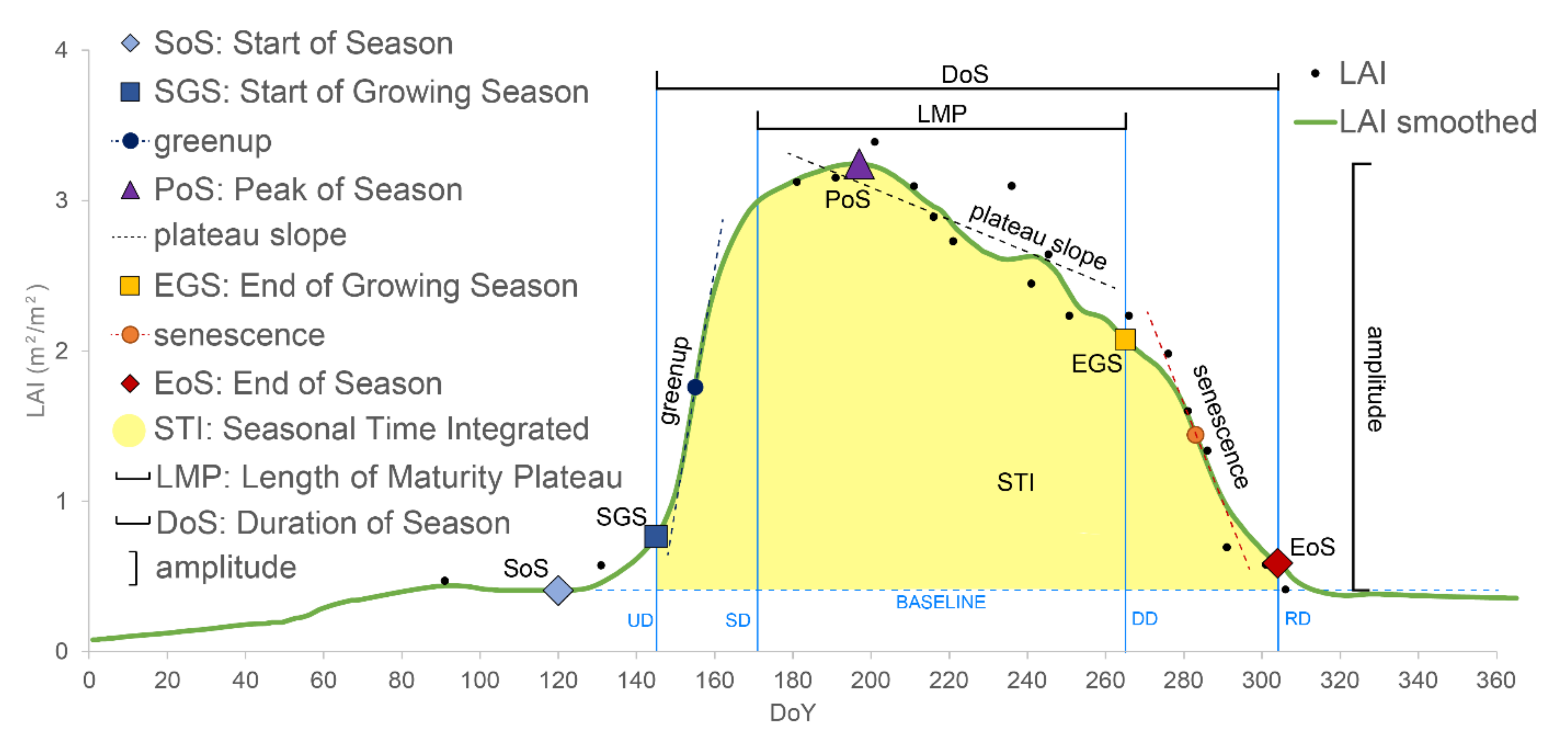
| Phenological metric | Time | Value | Acronym | Description |
|---|---|---|---|---|
| Start of Season | date, DoY | VI | SoS | Minimum VI value before the onset of photosynthesis |
| Start of Growing Season | date, DoY | VI | SGS | Beginning of measurable photosynthesis in the vegetation canopy |
| greenup | VI rate | greenup | Maximum positive slope of the curve during the onset of photosynthesis | |
| Peak of Season | date, DoY | VI | PoS | Maximum level of photosynthetic activity in the canopy during the growing season |
| End of Growing Season | date, DoY | VI | EGS | Beginning of significant degradation of chlorophyll revealing various accessory pigments |
| senescence | VI rate | senescence | Maximum negative slope of the curve during the chlorophyll degradation | |
| End of Season | date, DoY | VI | EoS | End of measurable photosynthesis in the vegetation canopy |
| Amplitude | VI | Amp | Maximum increase in canopy photosynthetic activity above the baseline | |
| Plateau slope | VI rate | plateau_slope | Slope during the maturity phase | |
| Duration of Season | days | DoS | Length of photosynthetic activity during the growing season | |
| Length of Maturity Plateau | days | LMP | Length of photosynthetic activity during the maturity phase | |
| Seasonal Time Integrated index | VI | STI | Canopy photosynthetic activity across the entire growing season calculated as daily integration of VI values |
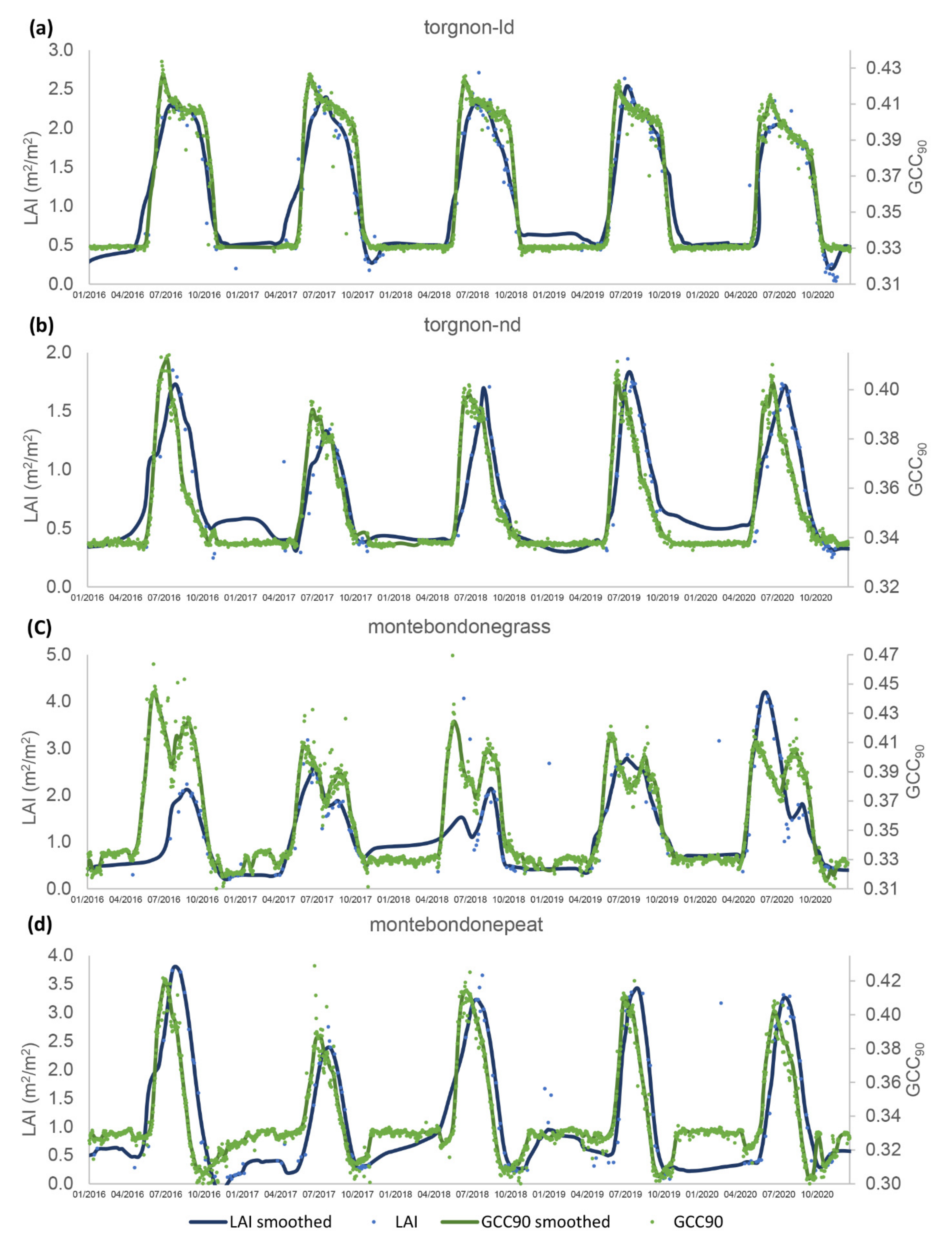
| Site Name | Ecosystem Type | Longitude | Latitude | Elevation |
|---|---|---|---|---|
| torgnon-ld | Deciduous Needleaved Forest | 7.5609 | 45.8238 | 2091 |
| torgnon-nd | Grassland | 7.5781 | 45.8444 | 2160 |
| montebondonegrass | Grassland | 11.0458 | 46.0147 | 1550 |
| montebondonepeat | Peatland | 11.0409 | 46.0177 | 1563 |
| ME | MAE | RMSE | r | |
|---|---|---|---|---|
| SGS | 6.35 | 14.47 | 17.71 | 0.6758 |
| PoS | −26.94 | 26.94 | 27.56 | 0.8804 |
| EGS | −1.18 | 14.59 | 18.06 | 0.8555 |
| EoS | −13.41 | 14.82 | 20.5 | 0.7645 |
| greenup | −3 | 17.94 | 22.19 | 0.4079 |
| senescence | −8.59 | 18.47 | 24.04 | 0.6242 |
Publisher’s Note: MDPI stays neutral with regard to jurisdictional claims in published maps and institutional affiliations. |
© 2022 by the authors. Licensee MDPI, Basel, Switzerland. This article is an open access article distributed under the terms and conditions of the Creative Commons Attribution (CC BY) license (https://creativecommons.org/licenses/by/4.0/).
Share and Cite
Filipponi, F.; Smiraglia, D.; Agrillo, E. Earth Observation for Phenological Metrics (EO4PM): Temporal Discriminant to Characterize Forest Ecosystems. Remote Sens. 2022, 14, 721. https://doi.org/10.3390/rs14030721
Filipponi F, Smiraglia D, Agrillo E. Earth Observation for Phenological Metrics (EO4PM): Temporal Discriminant to Characterize Forest Ecosystems. Remote Sensing. 2022; 14(3):721. https://doi.org/10.3390/rs14030721
Chicago/Turabian StyleFilipponi, Federico, Daniela Smiraglia, and Emiliano Agrillo. 2022. "Earth Observation for Phenological Metrics (EO4PM): Temporal Discriminant to Characterize Forest Ecosystems" Remote Sensing 14, no. 3: 721. https://doi.org/10.3390/rs14030721
APA StyleFilipponi, F., Smiraglia, D., & Agrillo, E. (2022). Earth Observation for Phenological Metrics (EO4PM): Temporal Discriminant to Characterize Forest Ecosystems. Remote Sensing, 14(3), 721. https://doi.org/10.3390/rs14030721