Evaluation of Agricultural Bare Soil Properties Retrieval from Landsat 8, Sentinel-2 and PRISMA Satellite Data

Abstract

The PRISMA satellite is equipped with an advanced hyperspectral Earth observation technology capable of improving the accuracy of quantitative estimation of bio-geophysical variables in various Earth Science Applications and in particular for soil science. The purpose of this research was to evaluate the ability of the PRISMA hyperspectral imager to estimate topsoil properties (i.e., organic carbon, clay, sand, silt), in comparison with current satellite multispectral sensors. To investigate this expectation, a test was carried out using topsoil data collected in Italy following two approaches. Firstly, PRISMA, Sentinel-2 and Landsat 8 spectral simulated datasets were obtained from the spectral resampling of a laboratory soil library. Subsequently, bare soil reflectance data were obtained from two experimental areas in Italy, using real satellites images, at dates close to each other. The estimation models of soil properties were calibrated employing both Partial Least Square Regression and Cubist Regression algorithms. The results of the study revealed that the best accuracies in retrieving topsoil properties were obtained by PRISMA data, using both laboratory and real datasets. Indeed, the resampled spectra of the hyperspectral imager provided the best Ratio of Performance to Inter-Quartile distance (RPIQ) for clay (4.87), sand (3.80), and organic carbon (2.59) estimation, for the spectral soil library datasets. For the bare soil reflectance obtained from real satellite imagery, a higher level of prediction accuracy was obtained from PRISMA data, with RPIQ ± SE values of 2.32 ± 0.07 for clay, 3.85 ± 0.19 for silt, and 3.51 ± 0.16 for soil organic carbon. The results for the PRISMA hyperspectral satellite imagery with the Cubist Regression provided the best performance in the prediction of silt, sand, clay and SOC. The same variables were better estimated using PLSR models in the case of the resampled hyperspectral data. The statistical accuracy in the retrieval of SOC from real and resampled PRISMA data revealed the potential of the actual hyperspectral satellite. The results supported the expected good ability of the PRISMA imager to estimate topsoil properties.

1. Introduction

There is an acknowledged requirement for up-to-date, spatially precise and inexpensive soil-mapping methods to monitor the soil properties of both agronomic and environmental interest and their related processes [1,2]. The spatial and temporal monitoring of soil properties is also highly significant, from both environmental and economic perspectives.

The physical link between soil components and the electromagnetic spectrum has allowed the for development of promising soil spectroscopy techniques for the estimation of soil properties in the laboratory, as well as progressively from airborne and satellite platforms. Satellite hyperspectral images offer an important advantage for monitoring soil properties from the field to the regional scale. The relationships between the soil reflectance spectrum in the optical range and soil mineralogy, chemical composition [3], soil organic matter content [4], soil water content [5], and soil particle size distribution [6] have led to the development of promising data-driven or physical-based methods of estimating soil properties [7]. This is due to the interaction of soil components with visible and infrared radiation that show specific absorption features in this spectral range [8,9,10]. For example, clay minerals have typical spectral features in a shortwave infrared region (SWIR) between 2170 and 2360 nm. Soil organic carbon (SOC) considerably influences the shape and nature of soil reflectance spectra [11]. It has specific spectral features [12] in the visible region with a wide absorption characteristic reported at around 664 nm [13], and in the SWIR region, principally due to the two principal organic compounds that influence the reflectance of lignin (between 1600 and 1800 nm and around 2100 nm) and cellulose (around 2100 nm) [13,14,15]. Moreover, the biochemical components of soil organic matter [2] have effects on the reflectance in the visible (400–700 nm) and NIR-SWIR (700–2500 nm) intervals [2,16] of the spectrum.

Spectral chemometrics models are particularly suitable for the precise quantification of soil properties [17]. These approaches make use of the whole spectrum to assess soil parameters, leading to an optimal selection of the bands and spectral range. The most widely used calibration techniques for developing these models are those relying on the Partial Least Squares Regression (PLSR) [2,8,18,19,20,21], which has been exceptionally valuable for developing models that comprise a significant number of predictor variables while considering the relationship between spectra and soil characteristics [22]. In order to handle big and spatially varied spectral libraries to estimate soil characteristics over a reduced area, numerous approaches, based mainly on the intensification of the estimation capacity of local samples, were considered [23,24,25]. Cubist Regression and random forest have been progressively utilized to model and predict soil variables at both local and regional scales [22,26].

Numerous soil spectroscopy studies have been carried out in the laboratory and proved effective in the estimation of soil properties, with a significant level of accuracy [9,27,28,29,30]. Spectral chemometrics for the prediction of soil properties was demonstrated to be relevant and accurate in the simultaneous prediction of several soil variables in the laboratory [31,32,33]. The results of [34] provided good SOC content predictions with PLSR models. The authors of [30] concluded that accurate and globally stable PLSR models for predicting soil variables can be developed from spectra acquired in the laboratory. While this approach provides an estimation of soil properties at specific sampling points, geo-statistical or interpolation techniques are essential to produce continuous spatial data, i.e., maps; therefore, the prediction accuracy tend to decrease in larger areas.

The strength of the relationships between spectral features and soil properties decreases from laboratory to satellite imaging spectroscopy [35]. This is mainly due to the combination of weather conditions and atmospheric attenuation, soil conditions, the scale, and the spectral resolution of the sensors. As new challenges arise in the quantification of soil properties, there is a continuing effort to meet these challenges and advance model precision [1]. Many recent scientific papers demonstrated the ability of, and the encouraging results obtained for, soil properties’ prediction and mapping from Sentinel-2 and Landsat 8 optical data [31,32,33,34].

The extensive Sentinel-2 and Landsat 8 time series also strengthen the possibility of detecting bare-soil areas in croplands and, accordingly, tracking soil properties across big districts. The respective short and moderate revisit times of the two satellite constellations increase the likelihood of obtaining cloud-free images and a high number of bare soil fields. This is particularly important in the soil imaging spectroscopy context, due to the narrow time window in which it is possible to observe bare soil in croplands. The use of multispectral imagery in small study areas, and considering only bare soils, proved to be successful. However, the quantitative prediction of soil parameters through the bare soil images attained from multispectral remote sensors was not optimized by a deficient spectral resolution [32,33], principally due to the lack of narrow bands in the SWIR region (i.e., the spectral interval influenced by the soil chromophores). This is of great importance for the prediction, for example, of clay, which can be estimated by exploiting well-distinguished spectral features between 2200 and 2400 nm that are related to the O-H stretch and metal-OH bends of the clay lattice of the most clay minerals in soil (e.g., kaolinite, montmorillonite and illite) [36]. These specific spectral features can only be detected by a hyperspectral sensor with an adequate spectral resolution in this region.

In this regard, hyperspectral remote sensing is a suitable technology to produce spatially precise topsoil mapping [15,37]. With the current and forthcoming availability of hyperspectral satellite sensors with an adequate signal to noise ratio (SNR), such as with the launch of PRecursore IperSpettrale della Missione Applicativa (PRISMA) [2,8] and the upcoming launch of EnMAP [1], the mapping of soil variables over large extents using imaging spectroscopy can be achieved. These sensors can regularly upgrade soil maps in bare-soil zones, a task that can only be obtained from existing low spectral resolution sensors at present [38]. Furthermore, several bands in the SWIR spectral interval of the forthcoming satellite hyperspectral imagers will presumably permit a more accurate prediction of soil parameters in comparison to current multispectral sensors.

There is an increasing number of papers concerning the estimation of soil variables exploiting resampled and/or simulated satellite hyperspectral data using statistical models [8,11,39]. Gomez et al. [11], while comparing prediction models of SOC using hyperspectral proximal and remote sensing data, revealed that the SOC map predicted using PLSR models showed a similarity with field observations, demonstrating the potential of combining hyperspectral remote sensing datasets and chemometrics models. Novel approaches to soil information retrieval have been proposed in the literature, based on simulated data from satellite hyperspectral sensors, which have already been launched or are to be launched soon. Castaldi et al. [21] showed that using simulated PRISMA datasets with an a priori recognition of the soil humidity classes can lead to a reduction in the error in clay estimation. Steinberg et al. [40] showed that simulated EnMAP hyperspectral satellite data allows for the prediction of iron oxide, clay, and SOC in topsoil with a minor reduction in soil estimate accuracy compared to the airborne scale, while still retaining, with PLSR, a satisfactory prediction accuracy. Castaldi et al. [20] investigated the abilities of seven multispectral and simulated hyperspectral satellite datasets to predict soil variables from PLSR models. Their results showed that, in the absence and with the addition of noise, the performances of hyperspectral data, presented by Ratio of Performance to Inter-Quartile (RPIQ) range, were significantly better compared to those of multispectral imagers for topsoil clay, sand, silt and SOC estimation. The authors of [2] obtained a reasonable SOC prediction accuracy from a local PLSR approach applied to simulated EnMAP satellite imagery.

Even though previous studies explored the abilities of actual PRISMA data in non-photosynthetic vegetation monitoring [41] and land-use monitoring [42], the ability of the PRISMA hyperspectral sensor in the soil domain has not been reported to date.

The objective of this study is to assess the potential of the PRISMA hyperspectral data for the prediction of topsoil properties over agricultural bare soil areas, in comparison with Sentinel-2 and Landsat 8 multispectral data. We selected two experimental agricultural areas in Italy and compared different processing approaches using both the soil spectral measurements elaborated in the laboratory and extracted from satellite imagers at the field level. For actual remote-sensing data, bare soil fields were identified based on pre-defined spectral indexes thresholds. Subsequently, the usefulness of spectra extracted from single date images was assessed.

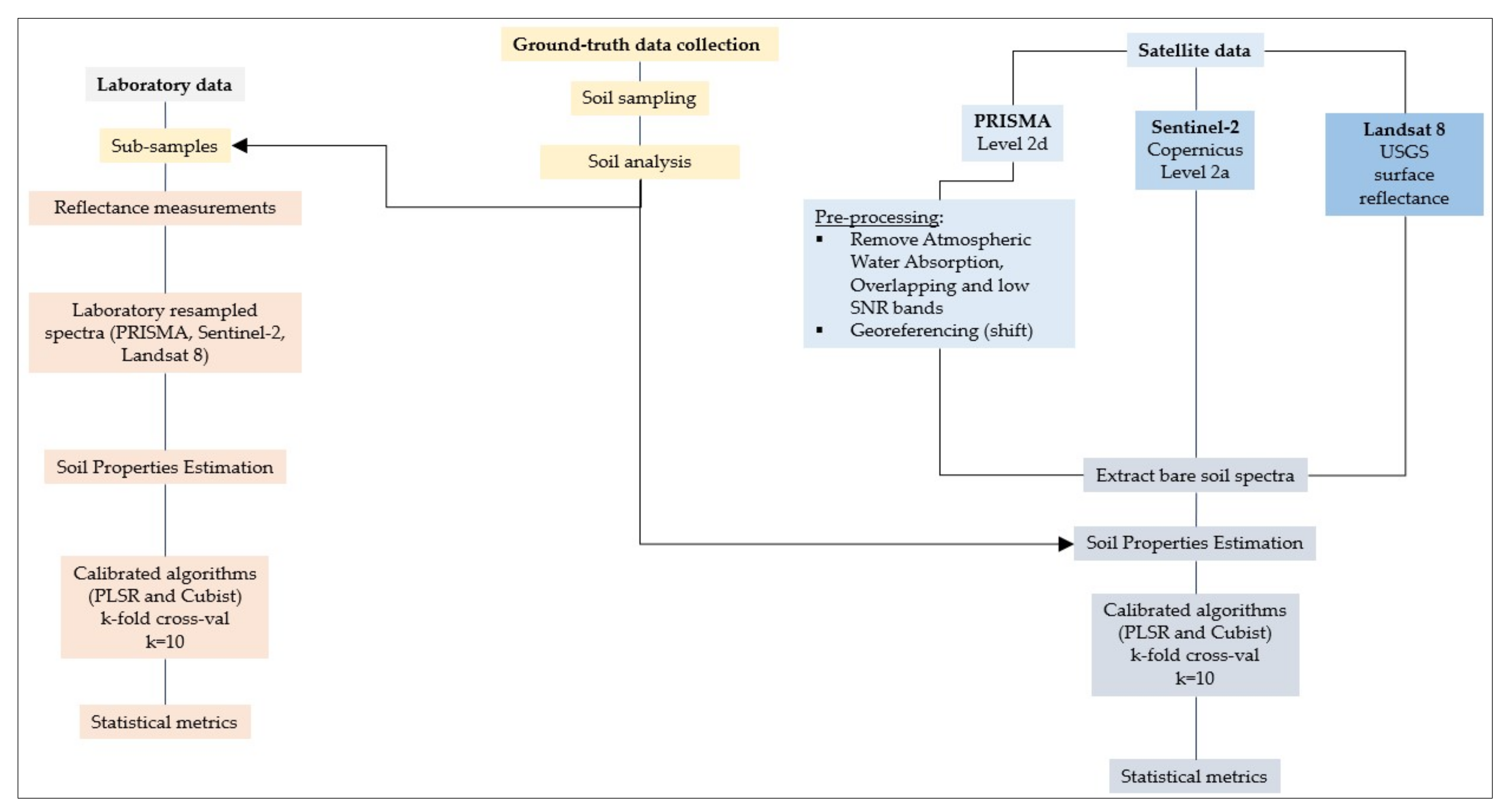
2. Materials and Methods

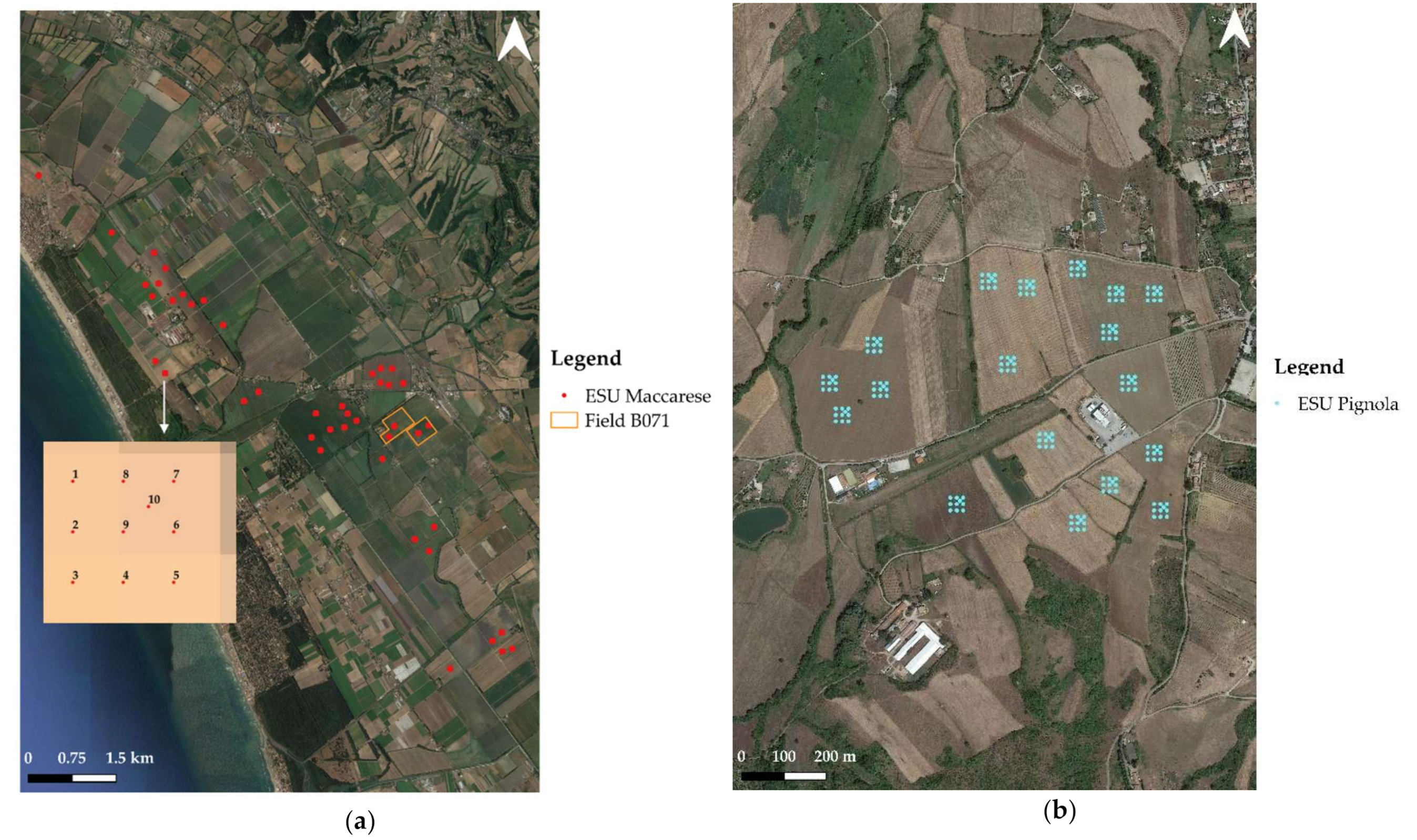
The flowchart of the methodology is illustrated in Figure 1 and hereafter, the following steps are described. These include: (A) soil sample collection and analysis (Section 2.2), (B) spectral laboratory measurements (Section 2.3); (C) pre-processing of the hyperspectral (Section 2.3.1) and multispectral (Section 2.3.2) remote sensing satellite data and (C) the prediction of soil properties based on bare soil spectra from both laboratory resampled data (Section 2.4.1) and collected satellite data (Section 2.4.2).

2.1. Study Area

Two agricultural test sites were selected for the estimation of topsoil properties in Central and Southern Italy.

For Central Italy, the area under investigation is located within the Maccarese S.p.A. farm (latitude 41°52′18″ N, longitude 12°14′05″ E, altitude 8 m a.s.l.) near Rome (Figure 2a). The study area underwent reclamation works in the early 1920s, which led to considerable changes to the landscape of the coastal marshland. The soil of this area is classified, according to a recent regional soil map [43], mainly as Dystric Arenosols (dunes and rear dune and recent alluvial and aeolian deposits) and Eutric Endochromic Luvisols (coastal plain reclaimed on fluvio-marsh sediments and recent fill), using the WRB FAO soil classification [43]. The Maccarese farm area is characterized by groups of beach ridges corresponding to eight homogeneous complexes that can be followed in both the Northern and in Southern part of the delta of the river Tevere and coastline dynamics. In particular, the soil parent materials of the Northeastern part of the studied site are alluvial deposits of the Arrone river. The main soil texture is sandy clay loam, which becomes more clayey towards the Northeast of the site; consequently, no carbonate topsoil is present in the area, while, on dunes, shell remnants can be present. The principal crops grown in the area are maize, followed by durum wheat, winter wheat, fava bean and forage crops.

The investigated area in Southern Italy is Pignola (Figure 2b) in the Basilicata Region (Latitude 40°33′45″ N, Longitude 15°45′40″ E). The sampled area altitudes vary from 720 to 760 m a.s.l. According to the Regional pedagogical map [44], which follows the WRB FAO soil classification, the Pignola soils correspond to Eutri-Vertic Cambisols (fluvio-lacustrine deposits of a local basin). The site is generally characterized by a moderately differentiated profile due to the partial removal of carbonates and browning of the horizons with free drainage. The main crop classes consist of arable land, pastures, and coppice woodland.

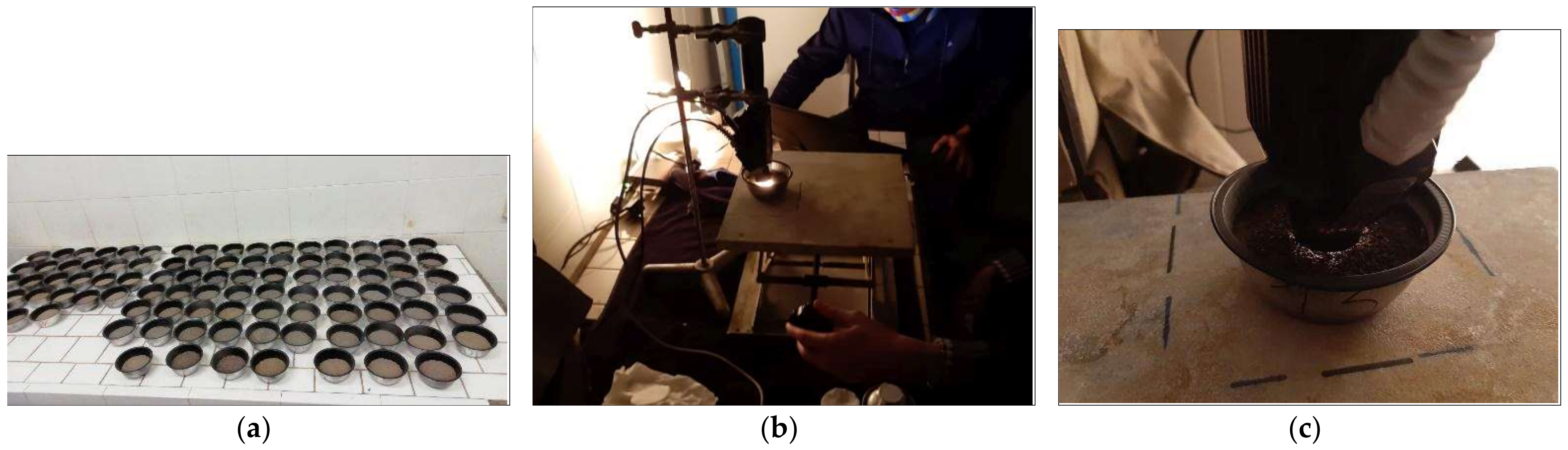
2.2. Field and Soil Sampling

Field campaigns were performed in both sites: for Maccarese on 11 November 2019, 28 January 2020 and 17 February 2020; for Pignola on 20 January 2020. The same protocol was followed, collecting soil samples located according to an Elementary Sample Unit (ESU) scheme set up to fit the PRISMA spatial resolution (

Table 1. Descriptive statistics (Min: Minimum; Max: Maximum; Mean; Std: standard deviation) of the measured soil properties at the two sampling sites for the 30 by 30 m ESU and for the 15 by 15 m sub-ESU.

		Maccarese		Pignola
		ESU (PRISMA, Landsat 8)	Sub-ESU (Sentinel-2)	ESU (PRISMA, Landsat 8)	Sub-ESU (Sentinel-2)
Clay (%)	Min	4.37	4.50	23.88	22.3
	Max	75.93	77.32	53.98	53.48
	Mean	37.56	37.33	33.99	33.78
	Std	21.10	21.13	7.28	7.20
Silt (%)	Min	1.05	0.70	30.85	30.77
	Max	28.89	29.26	46.82	48.45
	Mean	15.21	15.39	38.26	38.32
	Std	8.20	8.48	4.70	5.23
Sand (%)	Min	3.51	4.47	14.78	14.28
	Max	93.04	93.47	36.07	39.68
	Mean	47.23	47.27	27.75	27.9
	Std	26.88	26.86	6.53	7.05
SOC (%)	Min	0.18	0.22	0.96	0.96
	Max	2.09	2.08	1.80	1.83
	Mean	0.95	0.95	1.44	1.44
	Std	0.41	0.40	0.23	0.25

and

Table 2. Prisma satellite’s main characteristics.

	VNIR	SWIR	PAN
Spectral range	400–1010 nm	920–2500 nm	400–750
Spectral resolution	12 nm	12 nm
Spectral bands	66	171	1
SNR	>200:1 on 400–1000 nm >600:1 @ 650 nm	>200:1 in 1000–1750 nm >400:1 @ 1550 nm >100:1 in 1950–2350 nm >200:1 @ 2100 nm	>240:1
MTF	@ Nyquist Frequency > 0.3	@ Nyquist Frequency > 0.3	@ Nyquist Frequency > 0.2
Swath width	30 km; 2.77°
Spatial resolution	30 m	30 m	5 m
Telescope aperture	210 mm (diameter)
Orbital altitude	620 km

), i.e., according to 30 by 30 m quadrats. Each ESU contained 10 sampling points, positioned 15 m apart. On each point, three soil samples were collected within a 1 m radius, with an Ejkelkamp auger in the 0–10 cm depth layer. To optimize the sampling strategy on the PRISMA pixel size, the samples collected in the 10 ESU points were subsequently processed in the lab with two different sets of analyses. Soil samples from points 1 to 5 and samples from 6 to 9 were kept separate at the time of the laboratory analysis, thus obtaining two average soil properties values per ESU. The data of the points from 6 to 10 could be used as a 15 by 15 m sub-ESU, suitable for higher resolution sensors, e.g., compatible with the Sentinel-2 spatial scale, and to evaluate the variability within the ESU. We collected soil samples from a total of 61 ESU (43 from Maccarese and 18 from Pignola). Soil samples were analyzed to determine clay, silt, and sand content, using the pipette method, according to the USDA textural thresholds, and SOC content using the Walkley–Black method.

Table 1 shows the descriptive statistics of soil properties in the ESU and sub-ESU of the two experimental locations.

2.3. Laboratory Dataset

After air-drying, crushing, mixing, and sieving at 2 mm, a subsample of dry sieved soil was extracted from all soil samples that were originally collected in the field. The subsamples were placed in labeled small aluminum bowls, previously painted in black, on the interior. Reflectance measurements were performed across the 350–2500 nm range, using an Analytical Spectral Device (ASD, SN:6255) Field Spec Fr Pro spectroradiometer (ASD Inc., Denver, CO, USA), with a spectral resolution of 3 nm in the Vis-NIR range (350–1050 nm) and of 10 nm in the SWIR range (1050–2500 nm). The ASD was equipped with a contact probe containing a high-intensity quartz-halogen lamp (50 W) (Figure 3). Radiance across the 350–2500 nm spectral range was measured and converted to reflectance using a calibrated white Spectralon (Labsphere, Inc., North Sutton, NH, USA) reference panel. The protocol used for the measurements accurately followed the approach detailed in [1,28].

To prepare and control the experimental conditions, the ASD was turned on at least 60 minutes before the readings started, to warm up the spectrometers and the lamps. The room was kept dark during the readings to avoid any interference with the instrument. To prepare the soil sample readings, the following operations were performed: (i) mixing and flattening the soil within a bowl with a glass surface, (ii) bringing the samples to the ASD contact probe (CP) using an elevator, while the CP was held firmly in place, (iii) putting the soil in contact with the CP and perform the reading, and (iv) repeating the first three steps a total of 5 times per soil sample. Figure 3 illustrates the main phases of these operations. To correctly process the measurements, a check was performed every five sample readings to assess whether the white Spectralon panel had returned to 100%. If not, the white reference was reacquired to set it back to 100% to correct the detector’s drift. The soil standard samples of Lucky Bay and Wylie Bay [28] were also reacquired to standardize the ASD readings according to the standard protocol [28], to minimize the systematic effect of the measurements. The standardization followed the protocol set-up of Ben Dor et al. [28]. The five spectral replicates for each soil sample were averaged, and each spectrum was associated with the sample ID and its physical and chemical properties, constituting the laboratory dataset.

2.3.1. PRISMA Hyperspectral Data

The “PRecursore IperSpettrale della Missione Applicativa” (PRISMA), put in orbit from 2019 by the Italian Space Agency (ASI), is a technology demonstrator satellite mission finalized to develop user-driven [45] pre-operational products, taking advantage of the combination of a hyperspectral sensor and a panchromatic imagery. PRISMA mission is fully funded by ASI, while the payload was developed by the Italian Leonardo company. The main mission characteristics are described in the work of [46,47] and are briefly listed in Table 2.

PRISMA payload is a push-broom design based on a prism-based concept, acquiring 234 spectral bands in the 400–2500 nm spectral range. The first spectrometer provides 66 bands in the Vis-NIR spectral range, while the second spectrometer operates in the SWIR. The sun synchronous orbit obtains a swath of 30 km images with a Ground Sampling Distance (GSD) of 30 m, while PAN provides a co-registered image at 5 m/pixel. The revisit time is 29 days (from nadir), while shorter revisit times, of up to 7 days, could be managed by the available re-look capability. Mission lifetime is 5 years. The use of a prism as diffraction elements determines a non-uniform bandwidth across the Focal Plane Array (FPA). Moreover, as the center wavelength (CW) could change due to FPAs temperature each image is correlated by ancillary information indicating the proper CW and FWHM. Images are provided by ASI (https://prisma.asi.it/, accessed on 22 December 2021) in the Hierarchical Data Format–Earth Observing System (HDF-EOS5) format at different processing levels: L1 TOA radiance units, L2C ground reflectance without geometric correction, and L2D, corresponding to geocoded ground reflectance. Details of the ASI standard processing are available in the PRISMA Products Specification Document (ASI, PRISMA Products Specification Document Issue 2.1, accessed on 22 November 2021). The L2D processing level was selected for all the images utilized for the scope of this work.

The results presented in this study are based on the L2D (geocoded version of the level 2C “At-surface Reflectance Product”; [47,48]) data current version (i.e., 2.0.4) of PRISMA products distributed to the registered users by ASI. The requested L2D images (PRS_L2D_STD) were downloaded from the PRISMA mission catalog website (http://prisma-i.it, accessed on 22 December 2021). The PRISMA images used for this study were collected on the two test sites between November 2019 and August 2021 (see

Table 3. Dates of the PRISMA, Sentinel-2 and Landsat 8 satellite data employed for the two test sites of Maccarese and Pignola.

Study Area		PRISMA	Sentinel-2	Landsat 8
Maccarese	Calibration	7 November 2019	7 November 2019	1 November 2019
		8 February 2020	8 February 2020	5 February 2020
		20 October 2020	20 October 2020	18 October 2020
	Mapping	17 May 2021	15 May 2021	20 April 2018
Pignola	Calibration	23 August 2021	22 August 2021	20 August 2021

) with observer (roll±) angles varying from 4° to 18°. The overall weather conditions were stable, i.e., clear-sky conditions, during the days of acquisition (PRISMA image cloud coverage between 0.01% and 7.14%) with a very low aerosol presence during the field surveys.

The original HDF-EOS5 files were converted to Band Interleaved by Line (BIL) file format using an in-house tool developed in the IDL/ENVI 8.7.2. (L3Harris Technologies, Melbourne, FL, USA) by CNR IMAA (Italy) researchers. Before merging the two extracted Vis-NIR and SWIR hyperspectral datasets into a single image file, it was necessary to remove the overlapping reflectance bands in the 930–998 nm spectral range and remove the bands with a low SNR or those affected by noise.

From the original 234 bands, we excluded: (a) bands where the SNR was low (bands 1–9, i.e., 402–464 nm; bands after band 222, i.e., 2414 nm); (b) the atmospheric water absorption bands (bands 101–119 and 148–175, corresponding to the 1328–1523 nm and 1812–2044 nm spectral ranges, respectively); (c) bands in the overlapping zone (bands 59, 61, 63–70, i.e., 930–998 nm); and (d) bands with random spikes (band 44, i.e. 770 nm; bands 85–89, i.e. 1152–1196 nm) for each image, based on a visual comparison with the soil ground reflectance spectra, collected nearly simultaneously with the ASD FieldSpec Pro spectroradiometer (ASD Inc., Denver, CO, USA). The resulting dataset, with 150 reflectance bands, was used for all PRISMA images of this study.

Moreover, even though L2D PRISMA images are supplied and geocoded (in our case with Datum: WGS-84 and Projection: UTM 33 N), there is a residual, non-constant small shift (maximum 5 pixels) in all the images when compared to the ancillary digital cartography and vectorized shape file of the fields of interest. Therefore, we resampled all the images on the same grid of the field corners vectors, using a Nearest Neighbor algorithm implemented in the THOR Change Detection tool in ENVI 5.5.2. (L3Harris Technologies, USA). This was performed to co-register and align all the images (a) to set-up the data stack layer for the subsequent multitemporal analysis and (b) to allow for the accurate extraction of PRISMA spectra in correspondence to the ground-collected field soil samples.

2.3.2. Sentinel-2 and Landsat 8 Multispectral Data

Sentinel-2 Multi-Spectral Instrument (S2/MSI) and Landsat 8 Operational Land Imager (L8/OLI) data were obtained within the Google Earth Engine (GEE) environment for the two study areas, at dates very close to the PRISMA acquisitions (Table 3). The images were selected from the S2/MSI level 2A (COPERNICUS/S2_SR in GEE) and L8/OLI level 2, collection 2, Tier 1 (LANDSAT/LC08/C02/T1_L2 in GEE) image collections. Sentinel-2 pixels affected by clouds and clouds’ shadows were masked using the ‘QA60’ bitmask band for cirrus and opaque clouds, the ‘MSK_CLDPRB’ for clouds, and the ‘MSK_SNWPRB’ for snow. The cloudy Landsat 8 pixels were removed using the Pixel Quality Assessment Band. We selected B2 (central wavelength 490 nm), B3 (560 nm), B4 (665 nm), B5 (705 nm), B6 (740 nm), B7 (783 nm), B8 (842 nm), B8a (865 nm), B11 (1610 nm) and B12 (2190 nm) for S2/MSI and B2 (483 nm), B3 (560 nm), B4 (660 nm), B5 (865 nm), B6 (1650 nm), B7 (2220 nm) for L8/OLI.

2.4. Soil Properties’ Estimation

Soil property estimation models were built, starting from SOC, clay, sand, and silt content (dependent variables or outcomes) measured by chemical and physical analysis of the samples collected in the Maccarese and Pignola and the spectral data acquired in laboratory conditions or by satellite sensors (PRISMA, S2/MSI and L8/OLI), representing the independent variables or predictors. All estimation models were calibrated by testing two algorithms: Partial Least Square Regression (PLSR) [49] and Cubist [50]. The Cubist is a rule-based regression algorithm that allows a specific linear regression model to be defined for a subset of the calibration dataset. Therefore, the Cubist algorithm makes a partition at each node, characterized by a condition (rule) involving the independent variables, i.e., the soil spectral bands.

To reduce the noise of the actual PRISMA data and enhance the spectral features related to soil properties, the following spectral pre-treatments were tested: Savitzy–Golay filter (SG) [51], standard normal variate (SNV) [52] and continuum removal (CR) [36]. The model parameter tuning was conducted set up using the caret package in R [53], testing different numbers of components for PLSR and different combination of committees and neighbors for Cubist models. The best model was determined according to the lowest 10-fold cross-validation Root Mean Square Error (RMSE, Equation (1))

$$RMSE=\sqrt{\frac{{{\displaystyle \sum }}_{i=1}^n\left(y_m-y_p\right)}{n}}$$

(1)

where y_m are the soil properties’ measured values and y_p are the values predicted by the models. Each observation (measured value) appears in only one of the 10 folds selected for the cross-validation process. Thus, no overlap exists between groups, and the observations were split according to a pseudorandom number generator that allows for the output of the random fold-splitting to be reproduced to cross-validate all the predictive models.

To compare the estimation accuracy between soil properties and the other literature results, the coefficient of determination (R², Equation (2)), Ratio of Performance to Deviation (RPD, Equation (3)) and Ratio of Performance to Inter-Quartile distance [54] (RPIQ, Equation (4)) were computed

$${\mathrm{R}}^2=1-\frac{RSS}{TSS}$$

(2)

$$\mathrm{RPD}=\frac{Std}{\mathrm{RMSE}}$$

(3)

$$\mathrm{RPIQ}=\frac{IQ}{\mathrm{RMSE}}$$

(4)

where RSS is the sum of squares of the residuals, TSS is the total sum of squares, and Std and IQ are the standard deviation and the observed values, respectively. For each combination of outcome and predictors (e.g., SOC estimation using S2/MSI data), only the best model in terms of average 10-fold cross-validation Cubist and PLSR is reported in the manuscript. Moreover, in order to better compare the prediction accuracy obtained by bare soil satellite spectra, the standard error of the ten cross-validation folds is also provided for RPIQ and RPD values.

2.4.1. Laboratory and Resampled Spectra

The spectral library acquired by ASD Fieldspec Pro spectroradiometer in our laboratory under controlled conditions according to the Internal Soil Standard (ISS) [28] protocol was included in this work, as it might represent the best conditions for the estimation of soil properties, especially due to the very short distance from the sensor (contact probe) to the target object. Thus, the laboratory spectra were applied to evaluate the spectral resolution ability of the PRISMA, S2/MSI and L8/OLI sensors in ideal conditions, i.e., without disturbing factors affecting the satellite signal [31].

Four different spectral datasets were retrieved from the laboratory spectral library, and as many estimations models as soil properties (SOC, clay, sand, and silt): (i) all the spectral data provided by the ASD Fieldspec Pro spectroradiometer (hereinafter referred to as LAB), (ii) ASD spectra resampled according the PRISMA bands, excluding noisy bands, as described in Section 2.3.1 (hereinafter referred to as LAB PRISMA), (iii) ASD spectra resampled according to the S2/MSI bands (hereinafter referred to as LAB S2), and (iv) ASD spectra resampled according to the L8 bands (hereinafter referred to as LAB L8).

The resampling process was carried out with a Gaussian model, considering only the central wavelength and the bandwidth of each satellite band, using the spectral resampling function of the package hsdr in R [55]. This procedure provided a common method for all the satellites since a spectral response function was unavailable for PRISMA.

2.4.2. Bare Soil Satellite Spectra

For each soil sample collected in the Maccarese and Pignola areas, we selected the PRISMA image, among those listed as calibration in Table 3, that corresponded to the bare-soil conditions for the sampling areas. The selection was carried out by avoiding clouds, green and dry vegetation, thanks to the (a) agricultural management information, mainly provided by direct observations in the field, (b) visual check of the satellite images, (c) computation of the NDVI using a threshold of 0.35 to remove green vegetation pixels, and (d) the burn index 2 (NBR2; Equation (5)) to detect and remove non-photosynthetic vegetation (NPV) for S2/MSI and L8/OLI images

$$NBR2=\frac{{\rho }_{SWIR1 }-{\rho }_{SWIR2 }}{{\rho }_{SWIR1 }+{\rho }_{SWIR2 }}$$

(5)

where ${\rho }_{SWIR1 }$ is the reflectance value of B11 for S2/MSI (B11) and B6 for L8/OLI instrument, while ${\rho }_{SWIR2}$ corresponds to B12 for S2 and B7 for L8. Instead, we used the normalized cellulose absorption index (nCAI; Equation (6)) (nCAI < 0.03) for the PRIMA hyperspectral data. Compared to NBR2, this narrow band index is better suited to exploiting the of hyperspectral data’s ability to identify spectral features related to dry matter and cellulose [2,56,57] and, therefore, to detect NPV in the field.

$$nCAI=\frac{0.5\ast \left({\rho }_{2000}+{\rho }_{2200}\right)-{\rho }_{2100} }{0.5\ast \left({\rho }_{2000}+{\rho }_{2200}\right)+{\rho }_{2100}}$$

(6)

The bare-soil spectra were extracted according to the selected dates at different sampling point locations. For this study, we used the S2/MSI and L8/OLI images with the closest acquisition dates to the PRISMA dataset (Table 3).

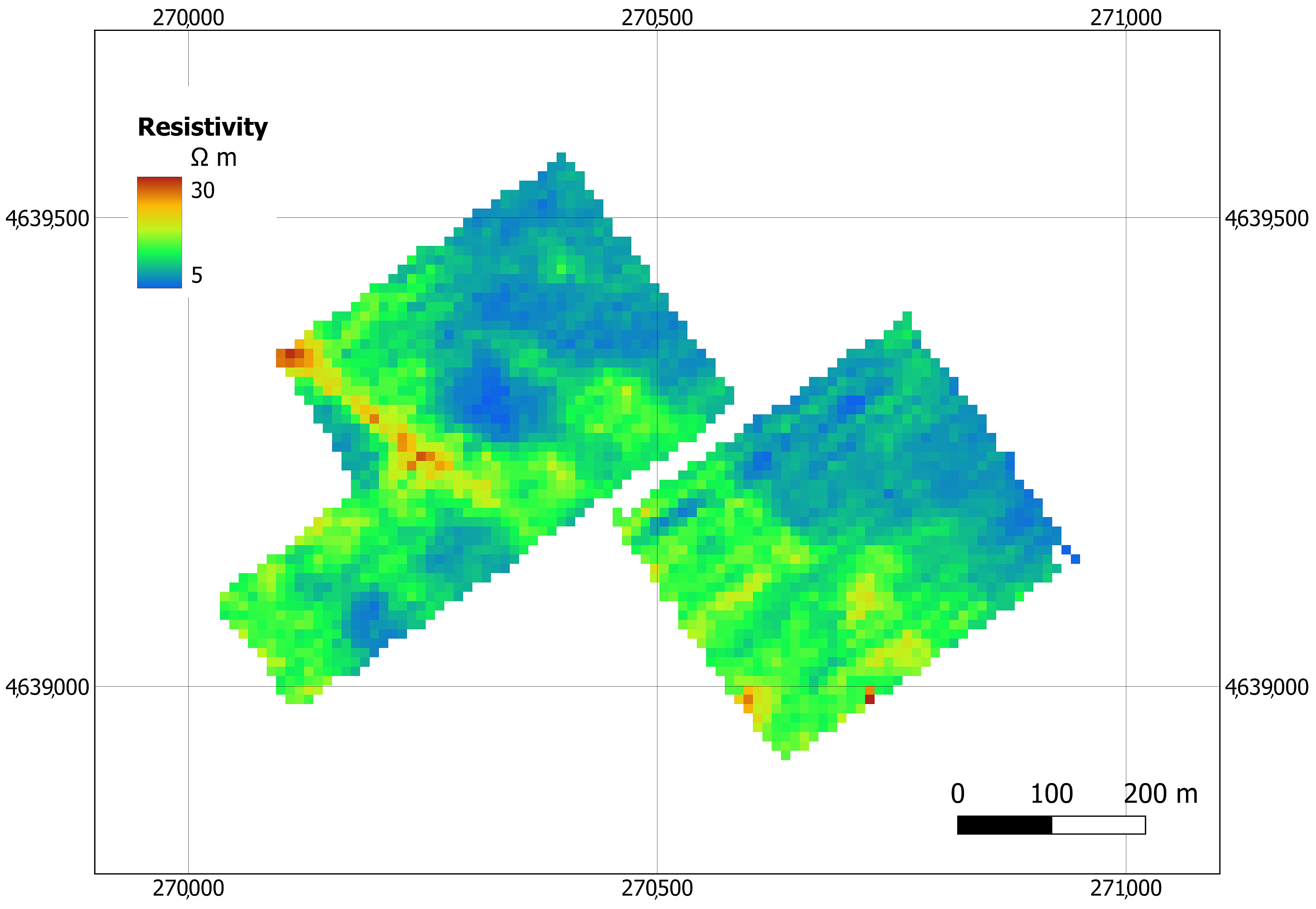
2.4.3. Spatial Assessment of Topsoil Maps

An assessment of the correspondence of estimated maps of SOC, clay, sand, and silt, with the pattern of spatial soil variability, was performed for an agricultural field within the Maccarese area (referred to as “Field B071” in Figure 2a), for which ground data on soil’s apparent electrical resistivity were available. The best models previously obtained for each soil property and satellite sensor were applied to independent satellite images, i.e., not those used for the calibration of the models (Table 3). For this purpose, we selected satellite images acquired in mid-spring 2021 for S2/MSI (15 May) and PRISMA (17 May), while, for L8/OLI, no cloud-free images were acquired in the same time window; consequently, we selected an image acquired at the same time of the year (mid-spring) in 2018, showing similar field conditions.

Each soil properties predictions map was spatially compared with the map obtained from a geoelectrical survey carried out on the field of the Maccarese farm area, since some soil properties, such as clay and SOC, are related to electrical resistivity/conductivity [58,59,60,61]. The geological survey acquired an apparent electrical resistivity (Ω m) of the 0–0.5 m topsoil layer at the meter resolution, using an Automatic Resistivity Profiling (ARP) multi-electrode continuous profiler, pulled by a quad. More specific information on the geoelectrical survey is provided by Casa et al. [62]. Resistivity maps were obtained by spatial interpolation of the ARP measurements using block kriging with block dimensions corresponding to the resolutions of PRISMA and Landsat (30 m) and Sentinel-2 (10 m). The satellite-derived maps of predictions were used as underlying grids for the interpolation. Figure 4 shows the ARP map obtained at Sentinel-2 resolution.

The spatial correlation between the resistivity maps and the maps of satellite-predicted soil properties was assessed using the Dutilleul t-test for the spatial processes [63,64] of the SpatialPack package implemented in R [65]. This test allows for an evaluation of the consistency of satellite-predicted maps, with the spatial patterns highlighted by the geophysical survey.

3. Results

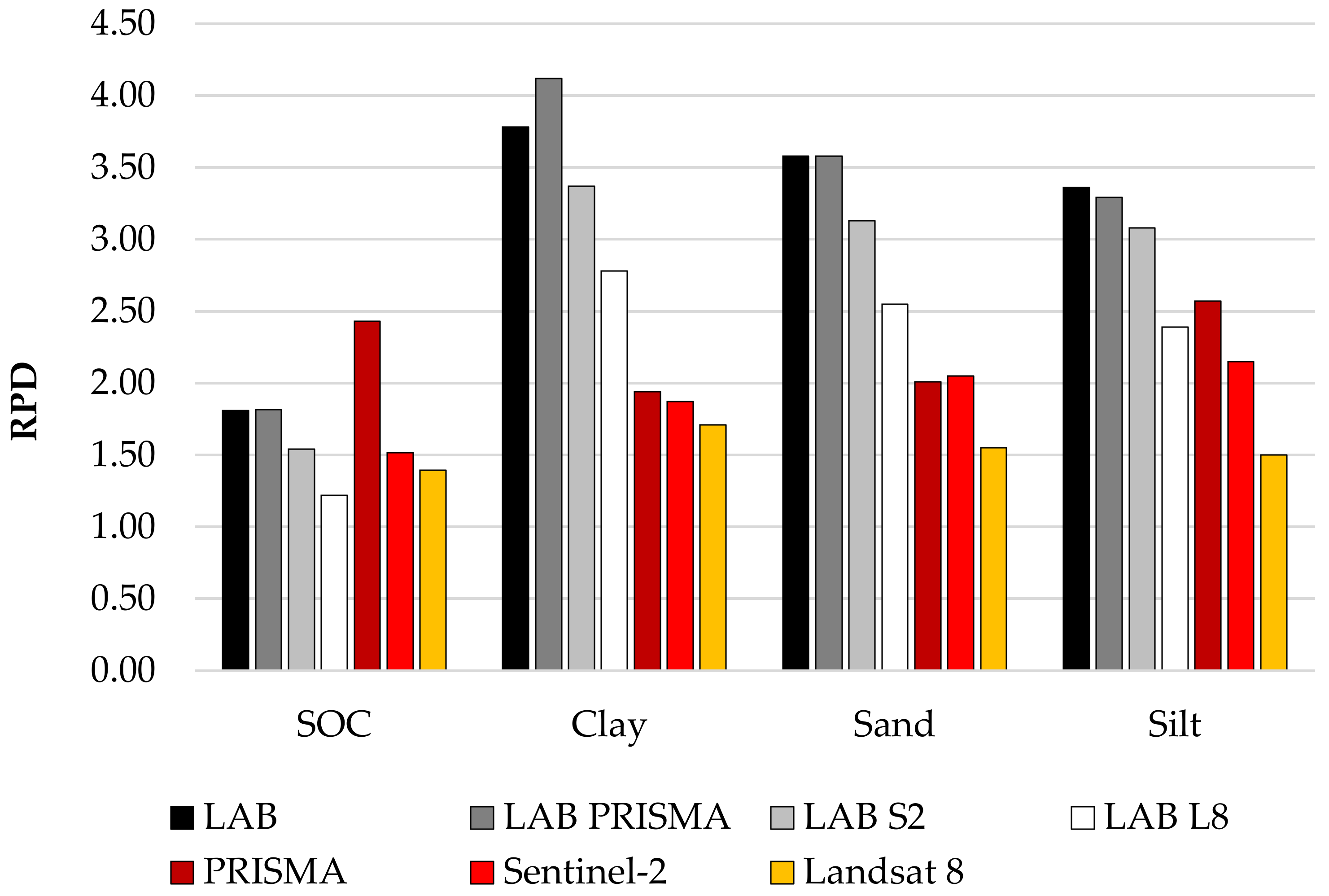
3.1. Soil Properties Estimation Using Laboratory and Resampled Spectra

The accuracy of the models resampled using laboratory spectra (LAB) was very high for clay (RPIQ: 4.46), sand (RPIQ: 3.79) and silt (RPIQ: 5.00), and lower for SOC (RPIQ: 2.59; RPD: 1.81; R²: 0.75) (

Table 4. Estimation accuracy of the best-performing prediction models of soil properties derived from laboratory resampled spectra. RMSE: Root Mean Square Error; R²: coefficient of determination; RPD: Ratio of Performance to Deviation; RPIQ: Ratio of Performance to Inter-Quartile distance.

Variable	Resampling Type	Model	RMSE (%)	RPIQ	RPD	R2
Clay	LAB PRISMA	PLSR	4.37	4.87	4.12	0.92
	LAB S2	Cubist	5.34	3.99	3.37	0.87
	LAB L8	Cubist	6.48	3.29	2.78	0.80
	LAB	PLSR	4.77	4.46	3.78	0.90
Silt	LAB PRISMA	PLSR	3.93	4.88	3.29	0.90
	LAB S2	Cubist	4.21	4.56	3.08	0.92
	LAB L8	Cubist	5.41	3.54	2.39	0.86
	LAB	PLSR	3.84	5.00	3.36	0.92
Sand	LAB PRISMA	PLSR	6.79	3.80	3.58	0.93
	LAB S2	Cubist	7.76	3.32	3.13	0.92
	LAB L8	Cubist	9.54	2.70	2.55	0.85
	LAB	PLSR	6.80	3.79	3.58	0.93
Organic Carbon	LAB PRISMA	PLSR	0.23	2.59	1.81	0.77
	LAB S2	PLSR	0.27	2.21	1.54	0.74
	LAB L8	Cubist	0.35	1.70	1.22	0.50
	LAB	PLSR	0.23	2.59	1.81	0.75

). The PLSR technique, in the case of the laboratory spectra, provided the best models for the retrieval of the four soil properties.

The spectra resampled according to the PRISMA bands (LAB PRISMA dataset) provided accurate estimation performances for the four soil properties. The best estimation accuracies were obtained for clay (RPIQ: 4.87; RPD: 4.12; R²: 0.92), sand (RPIQ: 3.80; RPD: 3.58; R²: 0.93) and SOC (RPIQ: 2.59; RPD: 1.81; R²: 0.77). The estimation accuracy of the three above-mentioned soil properties for LAB PRISMA data was the highest compared with the other laboratory datasets. The only exception was observed for silt estimation, with laboratory data that showed slightly higher results (RPIQ: 5.00; RPD: 3.36; RMSE: 3.84) than those achieved using PRISMA-simulated data (RPIQ: 4.88; RPD: 3.29; RMSE: 3.93).

By resampling the laboratory spectra according to the multispectral Sentinel-2 (LAB S2) and Landsat 8 (LAB L8) bands, the accuracy decreased for all the soil properties and particularly for sand in the case of LAB S2 (RMSE: 7.76; RPIQ: 3.32) and SOC in the case of LAB L8 (RMSE: 0.35; RPIQ: 1.70; RPD: 1.22; R²: 0.50). The models resampled to the Sentinel-2 data showed a good estimation accuracy for silt (RPIQ: 4.56; RPD: 3.08; R²: 0.92). The same property estimated using the LAB L8 data also provided a good degree of accuracy (RPIQ: 3.54; RPD: 2.39; R²: 0.86). Otherwise, LAB S2 data showed the best performances among multispectral datasets for all variables. For the LAB S2 and LAB L8 multispectral data, the best prediction accuracies were obtained using the Cubist method, except for SOC, where the PLSR provided the best results for the LAB S2.

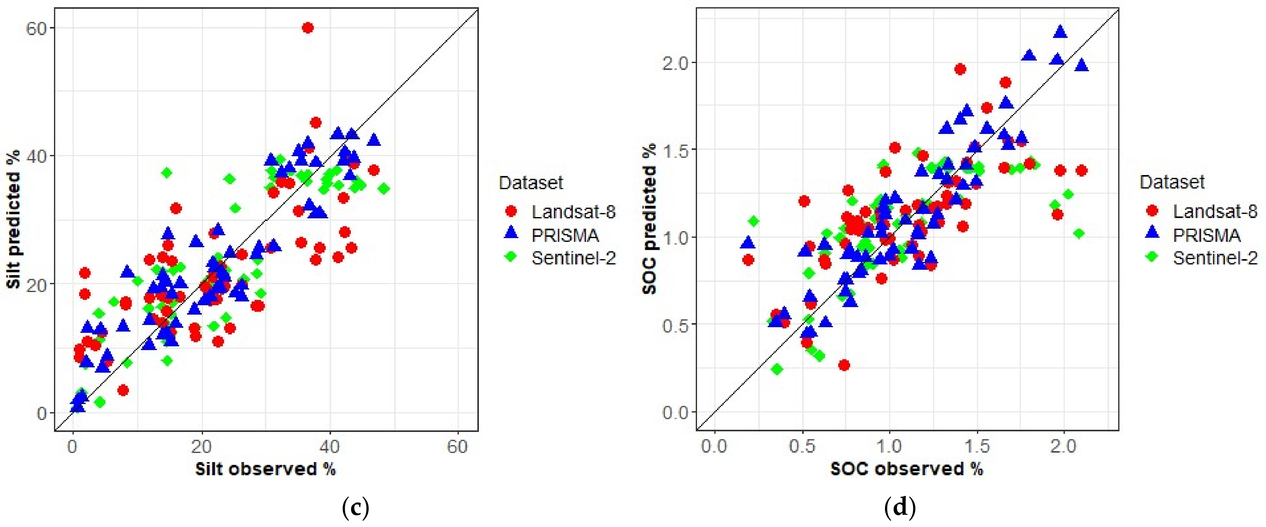
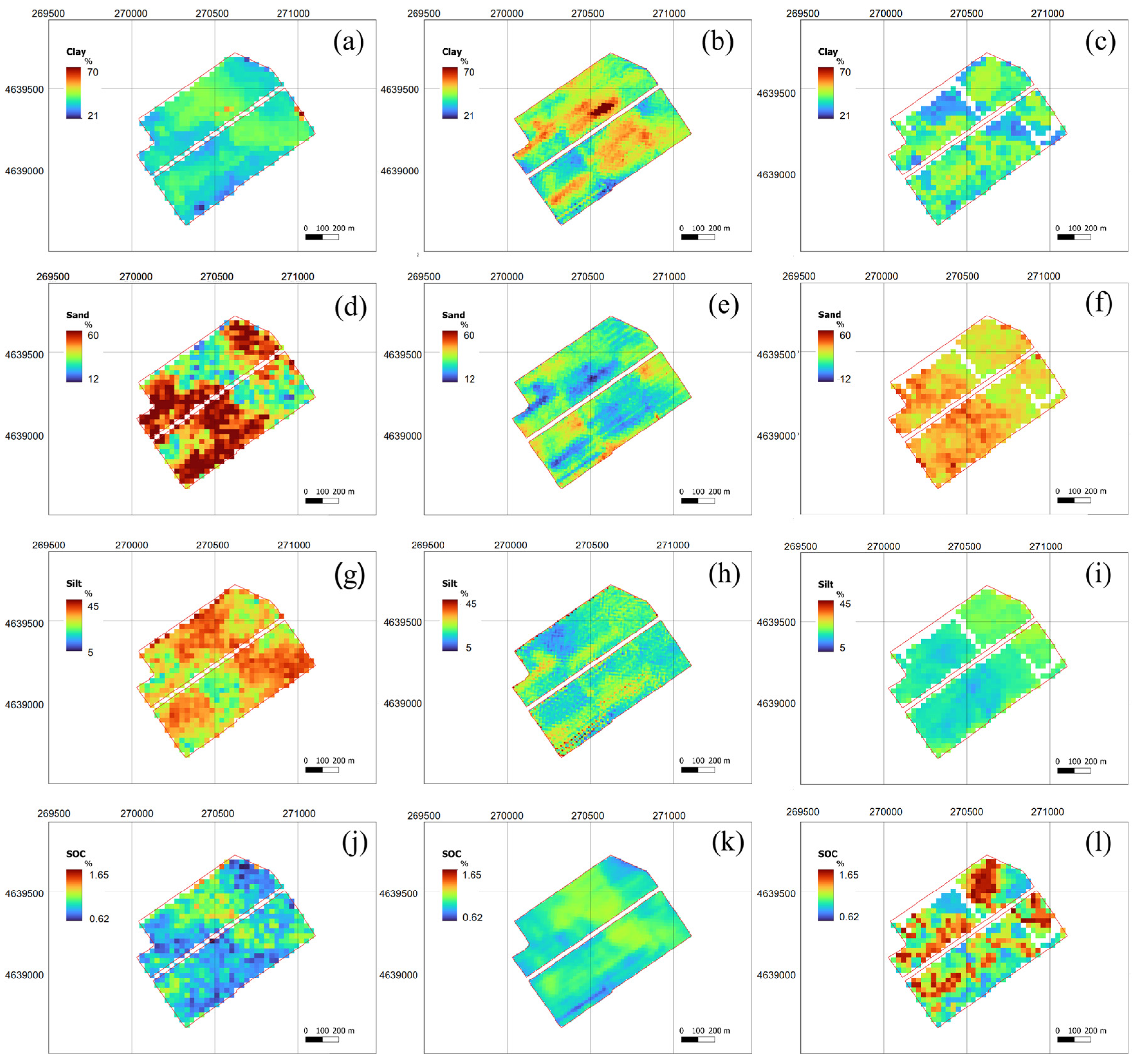
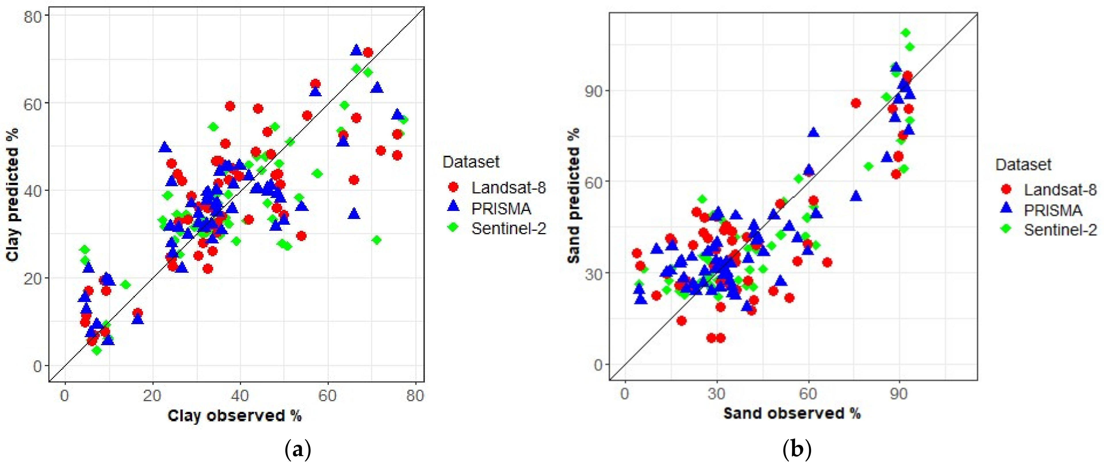
3.2. Soil Properties Estimation Using Bare Soil Satellite Spectra

As expected, the estimation accuracy with real satellite data decreased for all the soil properties as compared to the laboratory resampled spectra (

Table 5. Estimation accuracy of the best-performing prediction models for soil properties derived from Figure 2 and Landsat 8) spectra of bare soil. RMSE: Root Mean Square Error; R²: coefficient of determination; RPD: Ratio of Performance to Deviation; RPIQ: Ratio of Performance to Inter-Quartile distance; SE: standard error.

Variable	Satellite	Model	RMSE (%)	RPIQ ± SE	RPD ± SE	R2
Clay	PRISMA	Cubist	9.50	2.32 ± 0.07	1.88 ± 0.06	0.73
	Sentinel-2	Cubist	9.63	2.14 ± 0.17	1.87 ± 0.14	0.63
	Landsat 8	Cubist	10.58	2.01 ± 0.08	1.71 ± 0.07	0.61
Silt	PRISMA	Cubist	4.99	3.85 ± 0.19	2.57 ± 0.12	0.85
	Sentinel-2	PLSR	6.08	2.93 ± 0.10	2.15 ± 0.07	0.75
	Landsat 8	PLSR	8.59	2.24 ± 0.16	1.50 ± 0.11	0.68
Sand	PRISMA	Cubist	12.01	2.15 ± 0.05	2.01 ± 0.04	0.77
	Sentinel-2	PLSR	11.84	2.21 ± 0.10	2.05 ± 0.09	0.79
	Landsat 8	PLSR	15.72	1.64 ± 0.04	1.55 ± 0.04	0.58
Organic Carbon	PRISMA	Cubist	0.17	3.51 ± 0.16	2.43 ± 0.11	0.85
	Sentinel-2	PLSR	0.28	1.85 ± 0.20	1.52 ± 0.16	0.68
	Landsat 8	Cubist	0.30	1.98 ± 0.12	1.40 ± 0.08	0.60

). The worsening was particularly apparent for clay. However, the SOC model from PRISMA presented even better results than those obtained from LAB PRISMA data (RPIQ ± SE: 3.51 ± 0.16; RPD ± SE: 2.43 ± 0.11 for PRISMA and RPIQ: 2.59; RPD: 1.81 for LAB PRISMA).

The estimation of soil variables using hyperspectral PRISMA imagery provided the best results for soil texture and SOC estimation (Figure 5). The accuracy of the models using hyperspectral imagery was high for SOC (RPIQ ± SE: 3.51 ± 0.16; RPD ± SE: 2.43; RMSE: 0.17) and silt (RPIQ ± SE: 3.85 ± 0.19; RPD ± SE: 2.57± 0.12; RMSE: 4.99), and lower for clay (RPIQ ± SE: 2.32 ± 0.07; RPD ± SE: 1.88 ± 0.06; R²: 0.73).

The difference in statistical accuracy between hyperspectral and multispectral datasets became more apparent when using real satellite data, as compared with resampled laboratory data. The statistical accuracy obtained using the multispectral imagery was lower compared with those obtained using the hyperspectral image for all soil variables, except for sand, where the Sentinel-2 estimation model provided a slightly higher prediction accuracy (RPIQ ± SE: 2.21 ± 0.10; R²: 0.79) in comparison with PRISMA (RPIQ ± SE: 2.15 ± 0.05; R²: 0.77). The soil property models obtained using the Landsat 8 image provided a sufficient degree of accuracy (RPIQ ± SE: 2.01 ± 0.08; RPD ± SE: 1.71 ± 0.07 in the case of clay); however, all the L8/OLI statistics were worse than those obtained by S2/MSI data.

The RPD values obtained from hyperspectral and multispectral resampled data (Figure 6) for clay (RPD: 4.12 for LAB PRISMA and 3.37 for LAB S2) and sand (RPD: 3.58 for LAB PRISMA and 3.13 for LAB S2) estimation were significantly higher than those obtained with real spectra (case of clay: RPD is equal to 1.94 for PRISMA and 1.87 for Sentinel-2; case of sand: RPD is equal to 2.01 for PRISMA and 2.05 for Sentinel-2). Conversely, the estimation accuracy of SOC for the hyperspectral imager (RPD: 2.43) was statistically higher compared with the other laboratory (RPD: 1.81), resampled (LAB PRISMA RPD: 1.81) and real (Sentinel-2 RPD: 1.52) datasets.

In the absence of noise, and considering only the spectral characteristics, the performance of resampled hyperspectral data was significantly better than those of the resampled multispectral datasets. The PRISMA hyperspectral satellite data display a very similar behavior with respect to the laboratory spectral data when estimating all soil texture and SOC content variables (case of sand and SOC: RPD is equal to 3.58 and 1.81 for both LAB and LAB PRISMA, respectively).

For the SOC, clay and silt soil variables, the RPD confirmed the better estimation accuracy of the hyperspectral imager compared to the multispectral imagers. An exception was observed for sand estimation with Sentinel-2 data, which showed slightly higher results (RPD: 2.05) than those achieved using PRISMA (RPD: 2.01).

In more detail, we tested the application of the PLSR and Cubist Regression to laboratory resampled and real multispectral and hyperspectral satellite data to quantify the soil texture and SOC content. The results of the use of PRISMA hyperspectral satellite imagery with the Cubist Regression model provided the best-performing models for the prediction of clay, silt, sand and SOC. The variables silt, sand and SOC were better estimated using PLSR models in the case of the multispectral data. In this case, PLSR models performed better than those obtained using the Cubist Regression algorithm, which nevertheless produced the best soil texture and SOC maps when using resampled multispectral data. The PLSR algorithm provided the best predictor for use as an algorithm for soil texture and SOC content mapping over the study area using both the hyperspectral LAB and the resampled (PRISMA) datasets.

The best validated models using the different approaches (Cubist Regression and PLSR) were applied to the independent mapping images (Table 3) to draw soil texture and SOC maps (Figure 7).

Table 6. Analysis of spatial correlation between the resistivity data and the estimated soil properties. *** p < 0.001; ** p < 0.01; * p < 0.05; n.s. = not significant.

Soil Property	Sensor	Dutilleul’s Correlation	Significance
Clay	L8/OLI	0.35	*
	PRISMA	−0.67	***
	S2/MSI	−0.20	n.s.
Sand	L8/OLI	0.65	***
	PRISMA	0.58	**
	S2/MSI	0.01	n.s.
Silt	L8/OLI	−0.07	n.s.
	PRISMA	−0.51	**
	S2/MSI	0.35	**
SOC	L8/OLI	−0.04	n.s.
	PRISMA	−0.43	**
	S2/MSI	−0.67	***

presents an analysis of the spatial correlation between the resistivity map and the estimated soil properties. Dutilleul’s correlation between the ARP map and the estimated four soil properties from the hyperspectral sensor presented values of 0.58 for sand, −0.51 for silt, and −0.67 for clay. Clay and sand satellite-predicted maps presented a higher spatial correlation with the electrical resistivity when derived from PRISMA (Table 6) compared to those derived from S2/MSI. However, using L8/OLI, the spatial relationship was slightly higher for the case of sand-mapping results with a Dutilleul’s correlation of 0.65. The highest predicted sand contents, as well as medium predicted values at the center of the field (Figure 7d,f), highlighted a similar pattern for Landsat 8 and PRISMA platforms. Considering our results, the SOC map derived using the S2/MSI shows the highest spatial correlation, while a moderate correlation was obtained for SOC mapped from PRISMA data. Both multispectral (S2/MSI) and hyperspectral (PRISMA) sensor-derived SOC maps showed high spatial relationships with the geophysical survey results. Comparing the spatial distribution maps of SOC derived from both spaceborne sensors, data showed a similar pattern (Figure 7j,k).

4. Discussion

The results obtained in this study are a first attempt to assess the level of accuracy of the newly launched hyperspectral imager PRISMA for the estimation and mapping of bare-soil properties. For this purpose, PRISMA, S2/MSI and L8/OLI actual bare-soil spectra acquired in agricultural areas were used to build clay, silt, sand and SOC estimation models, and the three sensors were compared in terms of model prediction accuracy.

Topsoil clay content can generally be monitored by its mineralogical abundance and granulometry, and a high spectral resolution can be essential for detecting its specific wavelengths in the SWIR spectral region [29]. In this regard, the characteristic absorption features linked to the clay lattice are diverse, according to the composition of clay minerals in the soil, e.g., the main absorption features of kaolinite and montmorillonite are centered at 1400, 1900, and 2200 nm [66], while illite has two bands centered near 2300 and 2400 nm [20]. Therefore, as expected, as the S2/MSI and L8/OLI have both only two wide bands in the SWIR, their clay prediction accuracy is lower than that observed with laboratory resampled and real PRISMA imagery data (Table 4 and Table 5). In their research, Fongaro et al. [67] confirmed that spectral sensors with reduced bands, such as IKONOS, have low outcomes for clay estimate, as shown by the lower R² values. Castaldi [31] confirmed that neither S2/MSI nor L8/OLI could precisely predict the clay content, because of the low spectral resolution and large bandwidth (between 85 and 187 nm) of their SWIR bands, which prevent the exploitation of the narrow spectral features related to clay. The higher spectral resolution of PRISMA imagery could thus offer improvements in the assessment and mapping of clay content as compared to multispectral sensors. However, the improvement shown by PRISMA in this work, in terms of clay estimation, is more remarkable for resampled data (Table 4) than for actual satellite data (Table 5; Figure 6). This could be due to the lower SNR of the hyperspectral sensors in comparison to broad-band multispectral sensors. This SNR lowering is mainly due to energy accumulation in the narrow spectral bands of the hyperspectral sensors [20].

Figure 8 shows the percentage of times where each PRISMA band was used in a condition and/or a linear model of the Cubist algorithm for the estimation of soil properties. The clay prediction model used only visible and SWIR bands (Figure 8a), and wavelengths between 2100 and 2200 nm were largely used for both models and conditions, as expected, for the presence of the clay mineral spectral features in this spectral region.

Table 4 showed how LAB PRISMA spectra also provided the best results for sand and silt estimation, very close to those provided by LAB spectra. However, for clay, when moving from laboratory to actual satellite data, the differences between PRISMA and the two multispectral sensors became smaller (Table 5). For actual PRISMA data models, sand and silt showed an increased involvement of the spectral bands as compared to clay, for both Cubist conditions and models (Figure 8b,c). However, the visible region is crucial for all three soil texture properties. This is mainly due to the existing correlation between hue of soil and clay and sand percentage [20]. Generally, under equal moisture conditions and parental material, soil brightness (high reflectance values) is related to high sand percentage, while a dark hue (low reflectance values) can be related to high clay content. Fongaro et al. [67] used the Cubist model to test the bands’ importance for mapping soil attributes and highlighted the important contribution of the visible bands to sand estimation, as sand content is strongly related to the high albedo of quartz. In this regard, the study of [30] found a strong increase in reflectance in the NIR band of the Landsat 5 sensor for sandy soil, and this outcome is confirmed by Figure 8b, which shows how the NIR region for the PRISMA sensor is important for both Cubist conditions and models.

The SOC also affects the soil spectra in the visible range in the same direction of clay content, and Figure 8d clearly confirms the importance of the visible region for SOC estimation. In this regard, Reference [68] detected strong correlations between organic matter and reflectance, measured at 450, 590 and 664 nm. Shi et al. [18] explored the possibility of using hyperspectral remote sensing imagery to rapidly produce an SOC map at the regional scale, observing high variance importance projection (VIP) values in their PLSR model in the visible region between 400 and 600 nm. However, in Figure 8d, NIR and SWIR regions are also of great importance for the prediction; this is mainly due to the presence of overtones related to lignin between 1600 and 1800 nm and cellulose at around 2100 nm [68,69]. Moreover, other organic compounds of the organic matter, such as amide and aliphatic groups, can affect the spectral response at around 2300 nm.

The high importance of the SWIR bands in the prediction models, especially for SOC and clay, confirmed the good quality of the PRISMA sensor in this spectral region. This is an important improvement over the previous satellite hyperspectral sensors, particularly Hyperion, which showed strong limitations for clay content estimation due to their very low signal to noise ratio (SNR) in the SWIR, and especially at around 2200 nm, where the clay mineral features are located [20]. In our results, the best SOC estimation accuracy was obtained using PRISMA satellite imagery. PRISMA images showed the highest potential in terms of SOC prediction ability, even better than laboratory tests. This is probably a consequence of the conditions in which the image was acquired, where the pattern of soil moisture in the field may have played a role in the prediction of the SOC. In fact, spectral data collected under laboratory conditions were only computed under dry sample conditions. Casa et al. [39] showed that the presence of the spatial variability of soil moisture, at the time of remote sensing image acquisition, could improve the estimation of soil properties as compared to uniform dry soil conditions. While, for clay and sand, the difference in accuracy between PRISMA and the other sensors is not too evident, the hyperspectral sensor provided a strongly improved estimation accuracy for SOC (RPIQ: 3.51 ± 0.16) as compared to S2/MSI (RPIQ: 1.8 ± 0.20) and L8/OLI (1.98 ± 0.12). It should be noted that this difference is even more evident for high SOC values (>1.5%), which Sentinel-2 and the Landsat 8 model underestimated (Figure 5d).

Concerning the spatial distribution of the obtained soil maps, the analysis of spatial correlation between the resistivity data and the estimated soil properties showed a significant correlation with the geophysical survey for all the PRISMA maps, although the Landsat 8 and Sentinel-2 outperformed PRISMA for sand and SOC correlations, respectively (Table 6). Sentinel-2 SOC maps (Figure 7k) has a good inverse correlation with resistivity, probably due to the higher spatial resolution (10/20 m) in comparison with PRISMA and Landsat 8. However, the SOC patterns shown in Figure 7k are very similar to those obtained by PRISMA at a spatial resolution of 30 m (Figure 7j). Consequently, the spatial resolution of the PRISMA sensor does not seem to be a limiting factor for the estimation of soil properties for agricultural areas, especially where the spatial variability of soil properties does not occur within a very short range.

The high spectral resolution in the SWIR region of the PRISMA sensor allowed for the estimation of topsoil properties from bare soil images within the studied agricultural area; however, an investigation of the accuracy at other sites should be conducted. Future work will include different test areas in different soil regions to test the ability of PRISMA hyperspectral data to retrieve soil texture, SOC and other topsoil properties under different conditions (e.g., climate, soil types and soil moisture). The application of the PRISMA hyperspectral satellite to broad-scale mapping would be of great importance, considering other environmental covariates for a more robust modelling [70].

5. Conclusions

This research considers the ability of the hyperspectral sensor PRISMA in comparison with Sentinel-2 and Landsat 8 to predict and map soil texture and SOC content in two agricultural areas in Italy.

We obtained high prediction accuracies using simulated hyperspectral PRISMA datasets (RPIQ: 4.87 and 3.80 for clay and sand, respectively). The results were very similar to those of the full spectra (LAB) datasets, while a slight worsening was observed in terms of accuracy using spectra extracted from the real hyperspectral and multispectral spaceborne sensors.

A comparison between a resistivity map on a field of the study area and the soil texture and SOC maps retrieved from the best models applied to the PRISMA imagery revealed that the predicted maps are consistent with the patterns of variation in soil properties that were observed in the field, as confirmed by the high spatial correlation coefficients, especially for the case of clay and silt. Consequently, the medium spatial resolution of the PRISMA images (30 m) is not a limiting factor for mapping soil properties in the investigated area.

Our results indicate that PRISMA satellite hyperspectral data improved, in relative terms, the accuracy of soil variables’ estimation from bare-soil imagery, as compared to existing multispectral sensors with few and broad bands in the SWIR region. The higher spectral resolution of the hyperspectral imagery can exploit the well-defined narrow absorption spectral features characteristically linked to the functional sets in the Vis-NIR and SWIR spectral ranges associated with clay minerals and most important compounds, which constitute the organic matter in the soil. We conclude that hyperspectral data from the available PRISMA and the forthcoming satellite missions (e.g., EnMAP and CHIME) can advance the mapping and monitoring of soil texture and SOC as compared to the currently available imagers.

References

1. Chabrillat, S.; Ben-Dor, E.; Cierniewski, J.; Gomez, C.; Schmid, T.; van Wesemael, B. Imaging spectroscopy for soil mapping and monitoring. Surv. Geophys. 2019, 40, 361–399. [Google Scholar] [CrossRef] [Green Version]
2. Ward, K.J.; Chabrillat, S.; Brell, M.; Castaldi, F.; Spengler, D.; Foerster, S. Mapping soil organic carbon for airborne and simulated enmap imagery using the LUCAS soil database and a Local PLSR. Remote Sens. 2020, 12, 3451. [Google Scholar] [CrossRef]
3. Omran, E.S.E. Rapid prediction of soil mineralogy using imaging spectroscopy. Eurasian Soil Sci. 2017, 50, 597–612. [Google Scholar] [CrossRef]
4. Yuan, J.; Wang, X.; Yan, C.; Chen, S.; Wang, S.; Zhang, J.; Xu, Z.; Ju, X.; Ding, N.; Dong, Y.; et al. Wavelength selection for estimating soil organic matter contents through the radiative transfer model. IEEE Access 2020, 8, 176286–176293. [Google Scholar] [CrossRef]
5. Zeng, W.; Xu, C.; Huang, J.; Wu, J.; Tuller, M. Predicting near-surface moisture content of saline soils from near-infrared reflectance spectra with a modified Gaussian model. Soil Sci. Soc. Am. J. 2016, 80, 1496–1506. [Google Scholar] [CrossRef]
6. Sadeghi, M.; Babaeian, E.; Tuller, M.; Jones, S.B. Particle size effects on soil reflectance explained by an analytical radiative transfer model. Remote Sens. Environ. 2018, 210, 375–386. [Google Scholar] [CrossRef]
7. Norouzi, S.; Sadeghi, M.; Liaghat, A.; Tuller, M.; Jones, S.B.; Ebrahimian, H. Information depth of NIR/SWIR soil reflectance spectroscopy. Remote Sens. Environ. 2021, 256, 112315. [Google Scholar] [CrossRef]
8. Gomez, C.; Oltra-Carrió, R.; Bacha, S.; Lagacherie, P.; Briottet, X. Evaluating the sensitivity of clay content prediction to atmospheric effects and degradation of image spatial resolution using hyperspectral VNIR/SWIR imagery. Remote Sens. Environ. 2015, 164, 1–15. [Google Scholar] [CrossRef]
9. Lagacherie, P.; Baret, F.; Feret, J.B.; Madeira Netto, J.; Robbez-Masson, J.M. Estimation of soil clay and calcium carbonate using laboratory, field and airborne hyperspectral measurements. Remote Sens. Environ. 2008, 112, 825–835. [Google Scholar] [CrossRef]
10. Mutanga, O.; Skidmore, A.K.; Kumar, L.; Ferwerda, J. Estimating tropical pasture quality at canopy level using band depth analysis with continuum removal in the visible domain. Int. J. Remote Sens. 2007, 26, 1093–1108. [Google Scholar] [CrossRef]
11. Gomez, C.; Viscarra Rossel, R.A.; McBratney, A.B. Soil organic carbon prediction by hyperspectral remote sensing and field Vis-NIR spectroscopy: An Australian case study. Geoderma 2008, 146, 403–411. [Google Scholar] [CrossRef]
12. Liu, S.; Shen, H.; Chen, S.; Zhao, X.; Biswas, A.; Jia, X.; Shi, Z.; Fang, J. Estimating forest soil organic carbon content using Vis-NIR spectroscopy: Implications for large-scale soil carbon spectroscopic assessment. Geoderma 2019, 348, 37–44. [Google Scholar] [CrossRef]
13. Viscarra Rossel, R.A.; Lee, J.; Behrens, T.; Luo, Z.; Baldock, J.; Richards, A.; Viscarra Rossel, R.A.; Lee, J.; Behrens, T.; Luo, Z.; et al. Continental-scale soil carbon composition and vulnerability modulated by regional environmental controls. Nat. Geosci. 2019, 12, 547–552. [Google Scholar] [CrossRef]
14. Gholizadeh, A.; Saberioon, M.; Viscarra Rossel, R.A.; Boruvka, L.; Klement, A. Spectroscopic measurements and imaging of soil colour for field scale estimation of soil organic carbon. Geoderma 2020, 357, 113972. [Google Scholar] [CrossRef]
15. Gholizadeh, A.; Neumann, C.; Chabrillat, S.; van Wesemael, B.; Castaldi, F.; Borůvka, L.; Sanderman, J.; Klement, A.; Hohmann, C. Soil organic carbon estimation using VNIR–SWIR spectroscopy: The effect of multiple sensors and scanning conditions. Soil Tillage Res. 2021, 211, 105017. [Google Scholar] [CrossRef]
16. Demattê, J.A.M.; Dotto, A.C.; Paiva, A.F.S.; Sato, M.V.; Dalmolin, R.S.D.; de Araújo, M.d.S.B.; da Silva, E.B.; Nanni, M.R.; ten Caten, A.; Noronha, N.C.; et al. The Brazilian soil spectral library (BSSL): A general view, application and challenges. Geoderma 2019, 354, 113793. [Google Scholar] [CrossRef]
17. Ben-Dor, E. Quantitative remote sensing of soil properties. Adv. Agron. 2002, 75, 173–243. [Google Scholar] [CrossRef]
18. Shi, P.; Castaldi, F.; van Wesemael, B.; Van Oost, K. Large-scale, high-resolution mapping of soil aggregate stability in croplands using APEX hyperspectral imagery. Remote. Sens. 2020, 12, 666. [Google Scholar] [CrossRef] [Green Version]
19. Castaldi, F.; Chabrillat, S.; Jones, A.; Vreys, K.; Bomans, B.; van Wesemael, B. Soil organic carbon estimation in croplands by hyperspectral remote APEX data using the LUCAS topsoil database. Remote. Sens. 2018, 10, 153. [Google Scholar] [CrossRef] [Green Version]
20. Castaldi, F.; Palombo, A.; Santini, F.; Pascucci, S.; Pignatti, S.; Casa, R. Evaluation of the potential of the current and forthcoming multispectral and hyperspectral imagers to estimate soil texture and organic carbon. Remote Sens. Environ. 2016, 179, 54–65. [Google Scholar] [CrossRef]
21. Castaldi, F.; Palombo, A.; Pascucci, S.; Pignatti, S.; Santini, F.; Casa, R. Reducing the influence of soil moisture on the estimation of clay from hyperspectral data: A case study using simulated PRISMA data. Remote Sens. 2015, 7, 15561–15582. [Google Scholar] [CrossRef] [Green Version]
22. Dangal, S.R.S.; Sanderman, J.; Wills, S.; Ramirez-Lopez, L. Accurate and precise prediction of soil properties from a large mid-infrared spectral library. Soil Syst. 2019, 3, 11. [Google Scholar] [CrossRef] [Green Version]
23. Guerrero, C.; Zornoza, R.; Gómez, I.; Mataix-Beneyto, J. Spiking of NIR regional models using samples from target sites: Effect of model size on prediction accuracy. Geoderma 2010, 158, 66–77. [Google Scholar] [CrossRef]
24. Sankey, J.B.; Brown, D.J.; Bernard, M.L.; Lawrence, R.L. Comparing local vs. global visible and near-infrared (VisNIR) diffuse reflectance spectroscopy (DRS) calibrations for the prediction of soil clay, organic C and inorganic C. Geoderma 2008, 148, 149–158. [Google Scholar] [CrossRef] [Green Version]
25. Wetterlind, J.; Stenberg, B. Near-infrared spectroscopy for within-field soil characterization: Small local calibrations compared with national libraries spiked with local samples. Eur. J. Soil Sci. 2010, 61, 823–843. [Google Scholar] [CrossRef] [Green Version]
26. Pouladi, N.; Møller, A.B.; Tabatabai, S.; Greve, M.H. Mapping soil organic matter contents at field level with Cubist, random forest and kriging. Geoderma 2019, 342, 85–92. [Google Scholar] [CrossRef]
27. Viscarra Rossel, R.A.; Behrens, T.; Ben-Dor, E.; Brown, D.J.; Demattê, J.A.M.; Shepherd, K.D.; Shi, Z.; Stenberg, B.; Stevens, A.; Adamchuk, V.; et al. A global spectral library to characterize the world’s soil. Earth Sci. Rev. 2016, 155, 198–230. [Google Scholar] [CrossRef] [Green Version]
28. Ben Dor, E.; Ong, C.; Lau, I.C. Reflectance measurements of soils in the laboratory: Standards and protocols. Geoderma 2015, 245–246, 112–124. [Google Scholar] [CrossRef]
29. Adeline, K.R.M.; Gomez, C.; Gorretta, N.; Roger, J.-M. Predictive ability of soil properties to spectral degradation from laboratory Vis-NIR spectroscopy data. Geoderma 2017, 288, 143–153. [Google Scholar] [CrossRef] [Green Version]
30. Dematte, J.A.M.; Fiorio, P.R.; Ben-Dor, E. Estimation of soil properties by orbital and laboratory reflectance means and its relation with soil classification. Open Remote Sens. J. 2009, 2, 12–23. [Google Scholar] [CrossRef]
31. Castaldi, F. Sentinel-2 and landsat-8 multi-temporal series to estimate topsoil properties on croplands. Remote Sens. 2021, 13, 3345. [Google Scholar] [CrossRef]
32. Gholizadeh, A.; Žižala, D.; Saberioon, M.; Borůvka, L. Soil organic carbon and texture retrieving and mapping using proximal, airborne and sentinel-2 spectral imaging. Remote Sens. Environ. 2018, 218, 89–103. [Google Scholar] [CrossRef]
33. Castaldi, F.; Hueni, A.; Chabrillat, S.; Ward, K.; Buttafuoco, G.; Bomans, B.; Vreys, K.; Brell, M.; van Wesemael, B. Evaluating the capability of the sentinel 2 data for soil organic carbon prediction in croplands. ISPRS J. Photogramm. Remote Sens. 2019, 147, 267–282. [Google Scholar] [CrossRef]
34. Dvorakova, K.; Heiden, U.; van Wesemael, B. Sentinel-2 exposed soil composite for soil organic carbon prediction. Remote Sens. 2021, 13, 1791. [Google Scholar] [CrossRef]
35. Ben-Dor, E.; Chabrillat, S.; Demattê, J.A.M.; Taylor, G.R.; Hill, J.; Whiting, M.L.; Sommer, S. Using imaging spectroscopy to study soil properties. Remote Sens. Environ. 2009, 113, S38–S55. [Google Scholar] [CrossRef]
36. Clark, R.N.; Roush, T.L. Reflectance spectroscopy: Quantitative analysis techniques for remote sensing applications. J. Geophys. Res. 1984, 89, 6329–6340. [Google Scholar] [CrossRef]
37. Sun, W.; Liu, S.; Zhang, X.; Li, Y. Estimation of soil organic matter content using selected spectral subset of hyperspectral data. Geoderma 2022, 409, 115653. [Google Scholar] [CrossRef]
38. Mulder, V.L.; de Bruin, S.; Schaepman, M.E.; Mayr, T.R. The use of remote sensing in soil and terrain mapping—A review. Geoderma 2011, 162, 1–19. [Google Scholar] [CrossRef]
39. Casa, R.; Castaldi, F.; Pascucci, S.; Palombo, A.; Pignatti, S. A comparison of sensor resolution and calibration strategies for soil texture estimation from hyperspectral remote sensing. Geoderma 2013, 197–198, 17–26. [Google Scholar] [CrossRef]
40. Steinberg, A.; Chabrillat, S.; Stevens, A.; Segl, K.; Foerster, S. Prediction of common surface soil properties based on Vis-NIR airborne and simulated EnMAP imaging spectroscopy data: Prediction accuracy and influence of spatial resolution. Remote Sens. 2016, 8, 613. [Google Scholar] [CrossRef] [Green Version]
41. Pepe, M.; Pompilio, L.; Gioli, B.; Busetto, L.; Boschetti, M. Detection and classification of non-photosynthetic vegetation from PRISMA hyperspectral data in croplands. Remote Sens. 2020, 12, 3903. [Google Scholar] [CrossRef]
42. Hank, T.; Berger, K.; Wocher, M.; Danner, M.; Mauser, W. Introducing the potential of the EnMAP-box for agricultural applications using DESIS and PRISMA data. In Proceedings of the 41 IEEE International Geoscience and Remote Sensing Symposium (IGARSS 2021), Brussels, Belgium, 11–16 July 2021; IEEE: Piscataway Township, NJ, USA, 2021; pp. 467–470, ISBN 9781665403696. [Google Scholar]
43. Napoli, R.; Paolanti, M.; di Ferdinando, S. Atlante Dei Suoli Del Lazio; ARSIAL Regione Lazio: Rome, Italy, 2019; ISBN 978-88-904841-2-4. [Google Scholar]
44. Cassi, F.; Viviano, L. I Suoli Della Basilicata—Carta Pedologica Della Regione Basilicata in Scala 1:250.000. Regione Basilicata—Dip. Agricoltura e Sviluppo Rurale. Direzione Generale. Reg. Basilicata-Dip. Agric. Svilup. Rurale. Dir. Gen: Potenza, Italy, 2006; p. 343. [Google Scholar]
45. Schiavon, E.; Taramelli, A.; Tornato, A.; Pierangeli, F. Monitoring environmental and climate goals for european agriculture: User perspectives on the optimization of the Copernicus evolution offer. J. Environ. Manag. 2021, 296. [Google Scholar] [CrossRef]
46. Coppo, P.; Brandani, F.; Faraci, M.; Sarti, F.; Dami, M.; Chiarantini, L.; Ponticelli, B.; Giunti, L.; Fossati, E.; Cosi, M. Leonardo spaceborne infrared payloads for Earth observation: SLSTRs for Copernicus sentinel 3 and PRISMA hyperspectral camera for PRISMA satellite. Appl. Opt. 2020, 59, 6888. [Google Scholar] [CrossRef]
47. Loizzo, R.; Daraio, M.; Guarini, R.; Longo, F.; Lorusso, R.; Dini, L.; Lopinto, E. PRISMA mission status and perspective. In Proceedings of the IEEE International Geoscience and Remote Sensing Symposium (IGARSS), Yokohama, Japan, 28 July–2 August 2019; pp. 4503–4506. [Google Scholar]
48. Cogliati, S.; Sarti, F.; Chiarantini, L.; Cosi, M.; Lorusso, R.; Lopinto, E.; Miglietta, F.; Genesio, L.; Guanter, L.; Damm, A.; et al. The PRISMA imaging spectroscopy mission: Overview and first performance analysis. Remote Sens. Environ. 2021, 262. [Google Scholar] [CrossRef]
49. Wold, S.; Sjöström, M.; Eriksson, L. PLS-regression: A basic tool of chemometrics. Chemom. Intell. Lab. Syst. 2001, 58, 109–130. [Google Scholar] [CrossRef]
50. Quinlan, J.R. Learning with continuous classes. In Proceedings of the 5th Australian Joint Conference on Artificial Intelligence, Hobart, Australia, 16–18 November 1992; Word Scientific: Singapore, 1992; Volume 92, pp. 343–348. [Google Scholar]
51. Savitzky, A.; Golay, M.J.E. Smoothing and differentiation of data by simplified least squares procedures. Anal. Chem. 1964, 36, 1627–1639. [Google Scholar] [CrossRef]
52. Barnes, R.; Dhanoa, M.; Lister, S. Standard normal variate transformation and de-trending of near-infrared diffuse reflectance spectra. Appl. Spectrosc. 1989, 43, 772–777. [Google Scholar] [CrossRef]
53. Kuhn, M. Caret: Classification and Regression Training. R Package Version 6.0-90. 2010. Available online: https://CRAN.R-project.org/package=caret (accessed on 15 December 2021).
54. Bellon-Maurel, V.; Fernandez-Ahumada, E.; Palagos, B.; Roger, J.M.; McBratney, A. Critical review of chemometric indicators commonly used for assessing the quality of the prediction of soil attributes by NIR spectroscopy. TrAC Trends Anal. Chem. 2010, 29, 1073–1081. [Google Scholar] [CrossRef]
55. Lehnert, L.W.; Meyer, H.; Obermeier, W.A.; Silva, B.; Regeling, B.; Thies, B.; Bendix, J. Hyperspectral data analysis in R: The hsdar package. J. Stat. Softw. 2019, 89, 1–23. [Google Scholar] [CrossRef] [Green Version]
56. Chabrillat, S.; Eisele, A.; Guillaso, S.; Rogaß, C.; Ben-Dor, E.; Kaufmann, H. Hysoma: An easy-to-use software interface for soil mapping applications of hyperspectral imagery. In Proceedings of the 7th EARSeL SIG Imaging Spectroscopy Workshop, Edinburgh, Scotland, UK, 11–13 April 2011; pp. 11–13. [Google Scholar]
57. Nagler, P.L.; Inoue, Y.; Glenn, E.P.; Russ, A.L.; Daughtry, C.S.T. Cellulose absorption index (CAI) to quantify mixes soil-plant litter scenes. Remote Sens. Environ. 2003, 87, 310–325. [Google Scholar] [CrossRef]
58. Williams, B.G.; Hoey, D. The use of electromagnetic induction to detect the spatial variability of the salt and clay contents of soils. Soil Res. 1987, 25, 21–27. [Google Scholar] [CrossRef]
59. Sudduth, K.A.; Kitchen, N.R.; Wiebold, W.J.; Batchelor, W.D.; Bollero, G.A.; Bullock, D.G.; Clay, D.E.; Palm, H.L.; Pierce, F.J.; Schuler, R.T.; et al. Relating apparent electrical conductivity to soil properties across the North-Central USA. Comput. Electron. Agric. 2005, 46, 263–283. [Google Scholar] [CrossRef]
60. Triantafilis, J.; Lesch, S.M. Mapping clay content variation using electromagnetic induction techniques. Comput. Electron. Agric. 2005, 46, 203–237. [Google Scholar] [CrossRef]
61. Werban, U.; Kuka, K.; Merbach, I. Correlation of electrical resistivity, electrical conductivity and soil parameters at a long-term fertilization experiment. Near Surf. Geophys. 2009, 7, 5–14. [Google Scholar] [CrossRef]
62. Casa, R.; Castaldi, F.; Pascucci, S.; Basso, B.; Pignatti, S. Geophysical and hyperspectral data fusion techniques for in-field estimation of soil properties. Vadose Zone J. 2013, 12, 1–10. [Google Scholar] [CrossRef]
63. Dutilleul, P.; Clifford, P.; Richardson, S.; Hemon, D. Modifying the t test for assessing the correlation between two spatial processes. Biometrics 1993, 49, 305. [Google Scholar] [CrossRef]
64. Clifford, P.; Richardson, S.; Hemon, D. Assessing the significance of the correlation between two spatial processes. Biometrics 1989, 45, 123. [Google Scholar] [CrossRef]
65. Vallejos, R.; Osorio, F.; Bevilacqua, M. Spatial Relationships between Two Georeferenced Variables: With Applications in R; Springer Nature: Berlin/Heidelberg, Germany, 2020. [Google Scholar] [CrossRef]
66. Clark, R.N.; Rencz, A.N. Spectroscopy of rocks and minerals, and principles of spectroscopy. Man. Remote Sens. 1999, 3, 3–58. [Google Scholar]
67. Fongaro, C.T.; Demattê, J.A.M.; Rizzo, R.; Safanelli, J.L.; Mendes, W.S.; Dotto, A.C.; Vicente, L.E.; Franceschini, M.H.D.; Ustin, S.L. Improvement of clay and sand quantification based on a novel approach with a focus on multispectral satellite images. Remote Sens. 2018, 10, 1555. [Google Scholar] [CrossRef] [Green Version]
68. Ben-Dor, E.; Inbar, Y.; Chen, Y. The reflectance spectra of organic matter in the visible near-infrared and short wave infrared region (400–2500 nm) during a controlled decomposition process. Remote Sens. Environ. 1997, 61, 1–15. [Google Scholar] [CrossRef]
69. Castaldi, F.; Chabrillat, S.; Chartin, C.; Genot, V.; Jones, A.R.; van Wesemael, B. Estimation of soil organic carbon in arable soil in Belgium and Luxembourg with the LUCAS topsoil database. Eur. J. Soil Sci. 2018, 69, 592–603. [Google Scholar] [CrossRef]
70. Chen, S.; Arrouays, D.; Leatitia Mulder, V.; Poggio, L.; Minasny, B.; Roudier, P.; Libohova, Z.; Lagacherie, P.; Shi, Z.; Hannam, J.; et al. Digital mapping of GlobalSoilMap soil properties at a broad scale: A review. Geoderma 2022, 409, 115567. [Google Scholar] [CrossRef]
Figure 1. Flowchart of the proposed methodology.
Remotesensing 14 00714 g001
Figure 2. Study areas: (a) Maccarese: Central Italy and (b) Pignola: Southern Italy.
Remotesensing 14 00714 g002
Figure 3. Images from the laboratory spectroscopy experiment. (a) Painted trays with the soil samples; (b) Positioning of the sample below the sensor; (c) Close-up of the moment of contact between the ASD contact probe and the soil sample.
Remotesensing 14 00714 g003
Figure 4. Electrical resistivity map (10 m resolution) of the experimental field B071 of Maccarese, spatially interpolated using block kriging.
Remotesensing 14 00714 g004
Figure 5. (a) Clay, (b) sand, (c) silt and (d) SOC best model predictions for L8/OLI (red circles), PRISMA (blue triangles) and S2/MSI (green squares).
Remotesensing 14 00714 g005aRemotesensing 14 00714 g005b
Figure 6. Ratio of the Performance to Deviation (RPD) results for the laboratory (LAB), resampled and real hyperspectral and multispectral dataset mapping of the four soil properties (SOC, clay, sand, and silt).
Remotesensing 14 00714 g006
Figure 7. (a,d,g,j) PRISMA, (b,e,h,k) Sentinel-2 and (c,f,i,l) Landsat 8 soil texture and SOC maps retrieved from the best models applied to the 17/5/2021, 15/5/2021 and 20/4/2018 satellite imagery, respectively.
Remotesensing 14 00714 g007
Figure 8. The percentage of times where each PRISMA band was used in condition and linear models obtained by calibrating the Cubist models for clay (a), sand (b), silt (c) and SOC (d) content.
Remotesensing 14 00714 g008