Article

Estimating the Horizontal and Vertical Distributions of Pigments in Canopies of Ginkgo Plantation Based on UAV-Borne LiDAR, Hyperspectral Data by Coupling PROSAIL Model

Co-Innovation Center for Sustainable Forestry in Southern China, Nanjing Forestry University, Nanjing 210037, China
*
Author to whom correspondence should be addressed.
These authors contributed equally to this work and shared first authorship.
Remote Sens. 2022, 14(3), 715; https://doi.org/10.3390/rs14030715
Submission received: 6 December 2021 / Revised: 5 January 2022 / Accepted: 29 January 2022 / Published: 2 February 2022
(This article belongs to the Section Forest Remote Sensing)

Abstract

:
Pigments are the biochemical material basis for energy and material exchange between vegetation and the external environment, therefore quantitative determination of pigment content is crucial. Unmanned Aerial Vehicle (UAV)-borne remote sensing data coupled with radiative transfer models (RTM) provide marked strengths for three-dimensional (3D) visualization, as well as accurate determination of the distributions of pigment content in forest canopies. In this study, Light Detection and Ranging (LiDAR) and hyperspectral images acquired by a multi-rotor UAV were assessed with the PROSAIL model (i.e., PROSPECT model coupled with 4SAIL model) and were synthetically implemented to estimate the horizontal and vertical distribution of pigments in canopies of Ginkgo plantations in a study site within coastal southeast China. Firstly, the fusion of LiDAR point cloud and hyperspectral images was carried out in the frame of voxels to obtain fused hyperspectral point clouds. Secondly, the PROSAIL model was calibrated using specific model parameters of Ginkgo trees and the corresponding look-up tables (LUTs) of leaf pigment content were constructed and optimally selected. Finally, based on the optimal LUTs and combined with the hyperspectral point clouds, the horizontal and vertical distributions of pigments in different ages of ginkgo trees were mapped to explore their distribution characteristics. The results showed that 22-year-old ginkgo trees had higher biochemical pigment content (increase 3.37–55.67%) than 13-year-old ginkgo trees. Pigment content decreased with the increase of height, whereas pigment content from the outer part of tree canopies showed a rising tendency as compared to the inner part of canopies. Compared with the traditional vegetation index models (R2 = 0.25–0.46, rRMSE = 16.25–19.37%), the new approach developed in this study exhibited significant higher accuracies (R2 = 0.36–0.60, rRMSE = 13.53–16.86%). The results of this study confirmed the effectiveness of coupling the UAV-borne LiDAR and hyperspectral image with the PROSAIL model for accurately assessing pigment content in ginkgo canopies, and the developed estimation methods can also be adopted to other regions under different conditions, providing technical support for sustainable forest management and precision silvicuture for plantations.

1. Introduction

As an essential part of the forest ecosystem, planted forests play a significant role in maintaining the ecological environment, conserving biodiversity, and providing a variety of biochemical products for the ecosystem [1]. According to the China Forest Resources Report (2009–2013), the area of planted forests is approximately 7.95 × 10⁷ km2, accounting for approximately 32.94% of the national forest area [2]. Ginkgo (Ginkgo biloba L.) is a unique multi-purpose tree species in China, with important economic and ecological value [3]. As the principal component of the forest’s biochemical traits, total chlorophylls (Cab) and carotenoids (Car) can reflect the growth status of trees and environmental stress, and can also improve the understanding of the biochemical and physiological processes of trees [4]. The pigments in trees are controlled by many factors [5,6,7,8,9]. Despite that the shadow effect of canopies and the vertical heterogeneity of canopy structural parameters have been proved to impact significantly on the vertical distribution of pigment content within canopies, most current studies have regarded the canopy as a whole in the estimation of pigments [10,11]. Therefore, quantitative determination of pigments is essential not only to improve the understanding of the pigment distribution within canopies but also to monitor growth status. Although the conventional methods (such as organic solvent extraction and spectrophotometry determination) can obtain accurate determination of pigments, these extraction methods are usually time-consuming and destructive. Additionally, it is difficult to gain continuous distribution information on pigments on a larger scale, as this is limited to the field scale. In recent decades, numerous studies have proved that remote sensing can be used to accurately estimate biochemical traits at multiple scales [10,12,13]. As a commonly used remote sensing technology, Light detection and ranging (LiDAR) is capable of directly, rapidly and accurately providing three-dimensional (3D) information on objects’ surfaces (e.g., terrain and vegetation, etc.) by transmitting and recording laser signals. LiDAR has significant advantages in measuring the vertical structure of forests, which can be used to extract canopy structural parameters (e.g., tree position, tree height and canopy width, etc.) [14]. However, the LiDAR systems’ acquired data usually lacks spectral information for features on the ground [15,16]. While, hyperspectral images can provide the spectral reflectance signatures of forests and spectroscopic determination of pigments, it is difficult to provide vertical structural information [17]. Therefore, the synergistic use of LiDAR and hyperspectral data has the potential to obtain information on the 3D distribution of pigments in tree canopies.
Spectroscopic estimation of pigments usually comprises two approaches: empirical models and physical models [18]. Empirical models usually establish linear or nonlinear relationships between biochemical traits and spectra or their derivatives, which are often combined with spectral indices (SIs) [19,20]. However, these empirical relationships could be limited when applied to new datasets, leading to lack of robustness and causing uncertainties [4]. Thus, physical models have received increasing attention, having a reliable theoretical basis and strong robustness and can adapt to a variety of data. These physical models are developed based on the interaction between light and leaves, with the ability to simulate the transmission process of light in the leaf interior and canopy. As one of the physical models, Radiative transfer (RTM) can process forward and backward inversion to estimate biochemical or biophysical parameters. There are three main types of RTM models: leaf optical properties models [21,22,23,24,25,26,27], canopy optical properties models [28,29,30,31,32] and combined models [33,34,35,36,37,38]. PROSPECT is a widely used model within the first group [21], with specific professional versions to simulate the transmission of light in leaves. Previous studies have demonstrated that the PROSPECT-D model has marked reflectance simulation performance at the leaf scale, while the 4SAIL model has high robustness at the canopy scale [27,39,40]. Additionally, considering that the biochemical traits of leaves cannot be retrieved by canopy optical properties models alone, the PROSPECT model is usually coupled with canopy optical properties models (such as the PROSAIL model (i.e., PROSPECT model coupled with the 4SAIL model)) for scaling simulated leaf-scale reflectance to canopy-scale spectra [33].
Recently, PROSAIL has shown good potential in estimating pigments (e.g., Cab, Car, etc.) [33,41,42]. However, most relevant studies have focused on estimating only the horizontal distribution of pigments and were devoted to crops [43], as well as limited types of trees (e.g., Chinese fir and Poplar, etc.) [44], with the exception of Ginkgo trees. In order to fill the gap, this study explored the fusion of UAV-borne LiDAR datasets and hyperspectral images coupled with the PROSAIL model to estimate the 3D distribution of pigments in Ginkgo plantations. The specific research objectives are: (1) to select the optimal look-up tables (LUTs) based on the PROSAIL model calibrated to parameter characteristics of Ginkgo trees, (2) to evaluate the potential of coupling LiDAR and hyperspectral imaging data with the PROSAIL model for estimating pigments in individual Ginkgo trees with optimal LUTs, and (3) to characterize the horizontal and vertical distribution characteristics of pigments for Ginkgo plantations at different ages.

2. Materials and Methods

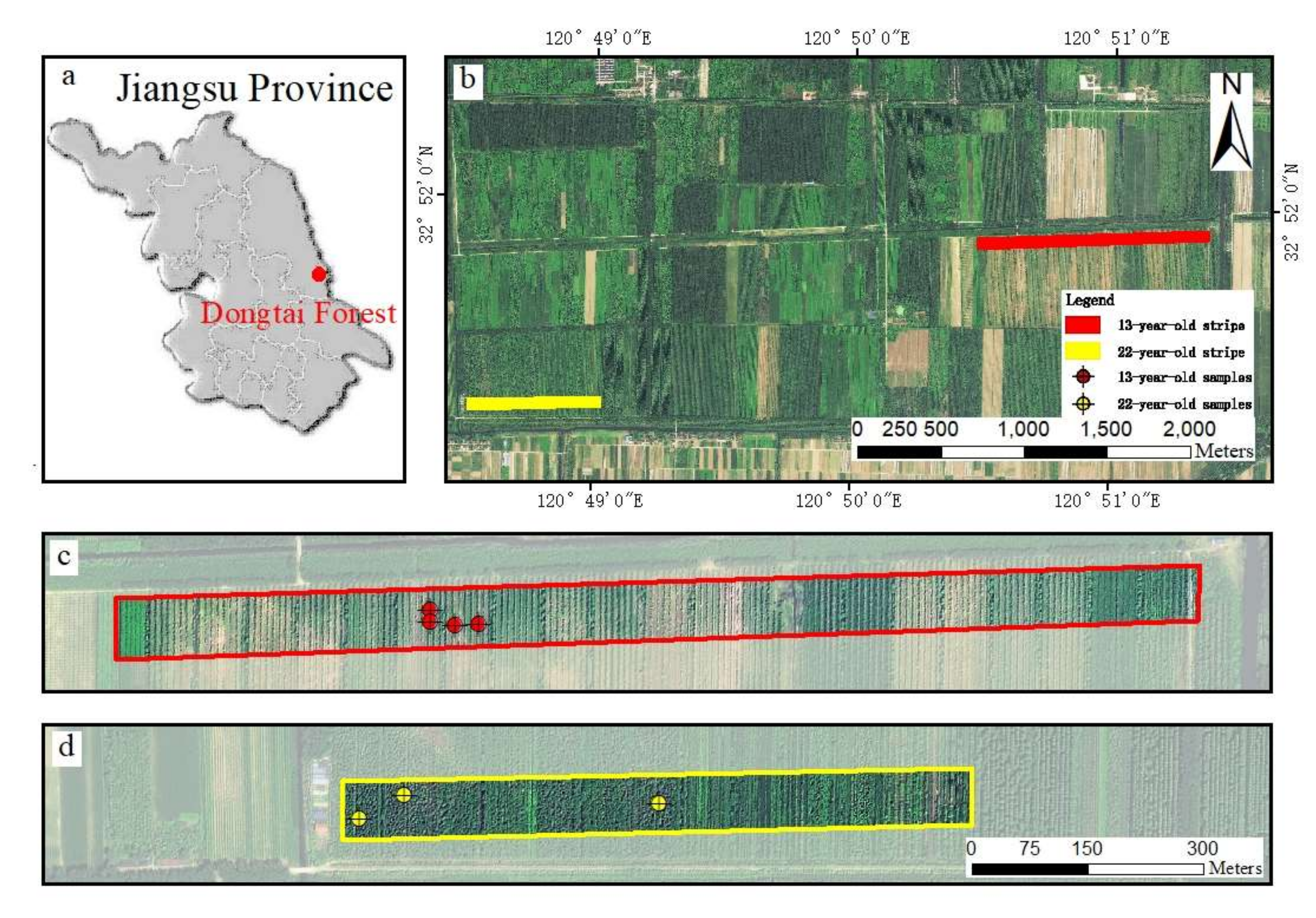
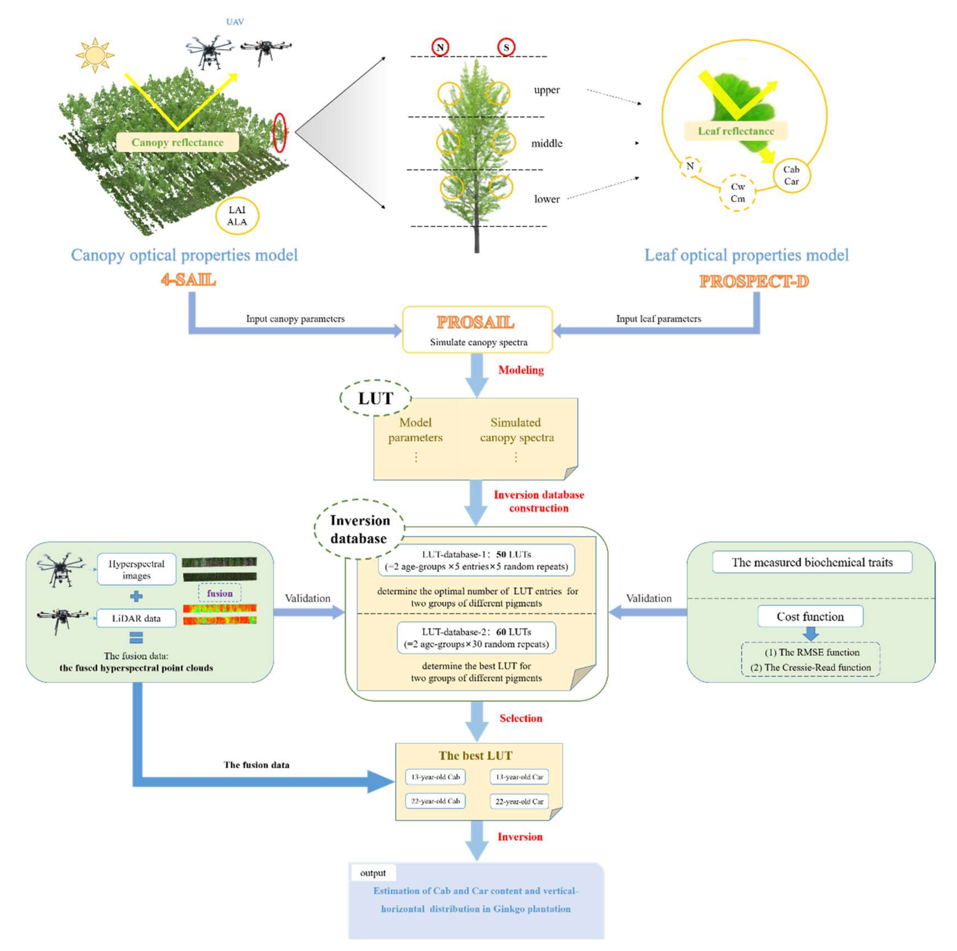
2.1. Study Area and Workflow

As a key coastal planted forest, Dongtai Forest (120°49′32.2″E, 32°52′20.6″N) is an essential multi-purpose forest plantation for wood production, marine disaster prevention, etc. The field covers approximately 2239 km2, and the forest coverage rate is around 85%. The vegetation types are mainly deciduous broad-leaved and needle-leaved forests, including mainly Ginkgo (Ginkgo biloba L.), Poplar Populus deltoides), and Dawn redwood (Metasequoia glyptostroboides). The Dongtai forest is located in a flat terrain, with an elevation range of between approximately 8–20 m. The annual average temperature and annual rainfall are approximately 14.6 °C and 1050 mm, respectively [45].
Within the forest stands of different ages (i.e., 13-year-old (young-aged) and 22-year-old (middle-aged)) and planting densities of Ginkgo trees, LiDAR and hyperspectral data were obtained separately including two UAV flight stripes (i.e., a LiDAR point cloud strip and a hyperspectral data strip) on 17–18 Aug. 2019. A total of seven sample trees were chosen for the study of biochemical traits’ extraction: (1) No.1–4 (13-year-old) (Figure 1c); and (2) No.5–7 (22-year-old) (Figure 1d). In this study, to represent different combinations of age, planting density (4 m × 4 m for 22-year-old trees; 2 m × 8 m for 13-year-old trees) and gender (male and female trees), four 13-year-old trees and three 22-year-old trees with typical cone shaped crowns were selected from Ginkgo plantations.
This study coupled UAV-borne LiDAR and hyperspectral imaging data with the PROSAIL model to map the horizontal and vertical distributions of pigments within the canopies of Ginkgo plantations. An overview of the workflow employed in this study is shown in Figure 2 and is mainly divided into three parts: (1) field data collection and measurement; (2) remote sensing data acquisition, processing and fusion; and (3) multi-LUTs generation from PROSAIL model and LUT-based inversion.

2.2. Data Collection and Processing

2.2.1. Field Data Collection and Measurement

The leaf samples were collected according to different heights and orientations (See Figure 2). According to the crown height of each sampling tree, the crown was divided into three equal vertical layers, namely, the upper, middle and lower canopy, respectively. Furthermore, each vertical layer was further separated into the northern crown and southern crown, thus a total of six parts were separated within the crown for analysis (3 vertical layers × 2 orientations: upper north, upper south, middle north, middle south, lower north and lower south). Seven sampling trees were divided into 42-part samples (7 sampling trees × 6 parts). In each part, approximately 100 leaves of the outside crown were collected using branch shears. For each part, 100 leaves were divided into two piles randomly (ten leaves: the pigment content was measured; other leaves: the water and dry matter content was measured). These collected leaves of 42 parts were placed separately on the sealed bag with labels and put in a box with ice, then sent to the laboratory for the extraction of pigment content. Pigment content of each part was measured by the organic solvent extraction method in the laboratory with ten leaves. We punched with a disk of 1.48 cm2, cut these disks into pieces and mixed then weighted 0.1 g pieces. These pieces were dipped in 10 mL of 96% ethanol to extract pigments until they turned completely white. The Specord®200 plus UV/Vis spectrophotometer [46] was used to measure the absorption values of chlorophyll a (Chla), chlorophyll b (Chlb) and carotenoids (Car) at 470, 649, and 665 nm wavelengths, respectively. According to the area of the disk (1.48 cm2), the specific leaf area (SLA) of each leaf sample was measured. Then, the mass-based Cab (mg·g−1) and Car (mg·g−1) were transformed to area-based Cab (μg·cm−2) and Car (μg·cm−2) content according to SLA.

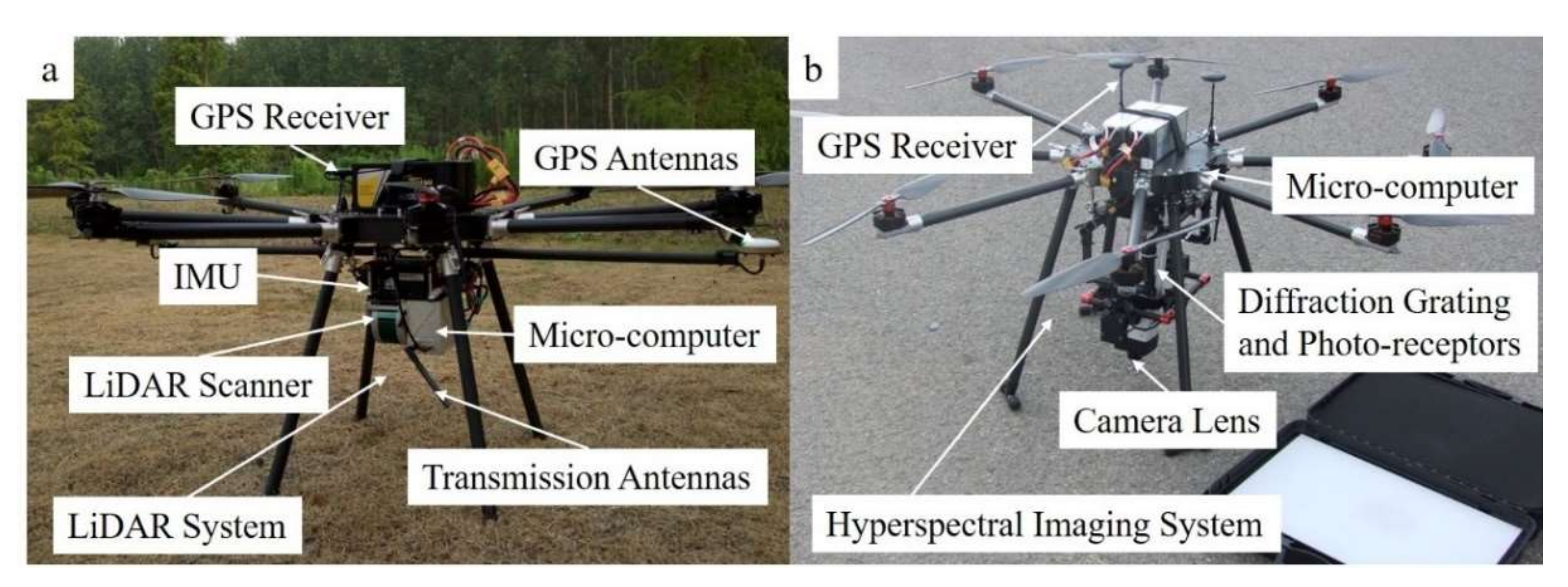
2.2.2. Remote Sensing Data Acquisition and Processing

LiDAR data (Figure 3a) and hyperspectral images (Figure 3b) were acquired by the GV1300 multi-rotor UAS platform on 17 and 18 Aug. 2019, respectively. The flight parameters and UAV-LiDAR system properties are shown in Table 1.
The LiDAR data were captured using a Velodyne Puck VLP-16 scanner at an elevation of 80 m above ground level with a flight speed of 6 m·s−1 on 18 Aug. The obtained LiDAR original data were processed by point cloud denoising, filtering, classification and normalization. Combining the IMU data with GPS data recorded by the base station and UAV platform, point coordinates were calculated. The digital surface model (DSM) and digital elevation model (DEM) with a resolution of 0.18 m were generated by the irregular triangulation network (TIN) algorithm for the pre-processing and hyperspectral images co-registration. The processing LiDAR point cloud adopted the point cloud segmentation method to segment the seven sampling trees and obtain the corresponding six part LiDAR point clouds for each sampling tree. In addition, the boundaries corresponding to each part-point-clouds for seven sampling tree were determined by manual delineation.
Hyperspectral images with 0.18 m spatial resolution of the 13-year-old and the 22-year-old Ginkgo plantations were obtained at 10.00 a.m. and 16.00 p.m. on Aug. 17, respectively. The images (spectral range = 403–929 nm, spectral resolution = 2.3 nm) were obtained by the ZK-VNIR-FPG480 imager at 80 m altitude above ground level with a flight speed of 4.8 m·s−1. A standard whiteboard was used to convert image brightness value (DN value) to spectral reflectance from the imagery. Then, the Savitzky-Golay filter (S-G filter), a weighted moving average filtering system, was used for reflectance image smoothing and denoising [47]. Specifically, S-G filtering was carried out in an IDL environment with a frame size of 5 data points (2nd degree polynomial) [48]. Due to the influence of random noise in the process of hyperspectral image collection, the 172 bands within the spectral range of 450 nm to 850 nm were retained for further analysis.
Before carrying out the remote sensing data fusion, the pre-processing hyperspectral images co-registration was carried out using the DSM created from the processing of the LiDAR point cloud. To make sure the fusion performance of the hyperspectral images and the processing LiDAR point cloud had the highest spatial consistency, in the co-registration two ground control points were randomly selected for each area of 5 × 5 m2 from both the hyperspectral images and the DSM data. The accuracies of co-registration for hyperspectral images were both less than 9 cm (half a hyperspectral image pixel).

2.2.3. Remote Sensing Data Fusion

The DSM-based approach, proposed by Shen et al. (2020) [45], was adopted to fuse the processing LiDAR point cloud and co-registered hyperspectral images. This fusion approach can accommodate the lack of spectral information in LiDAR and the lack of canopy structure information in hyperspectral data. Firstly, the LiDAR point clouds were divided into columns (0.18 m × 0.18 m × 30 m) consistent with the pixel grid of the hyperspectral images in the horizontal orientation. Secondly, for each column, the highest LiDAR point cloud was retained, while excluding other point clouds. Finally, the hyperspectral reflectance value of the corresponding pixel grid was distributed to the highest LiDAR point cloud within each column. Thus, the fused hyperspectral point clouds were obtained, containing spectra and structural information. The reflectance of fused hyperspectral point clouds within six parts for each sampling tree was simplified as the point-based reflectance.

2.2.4. Extracting Profile Characteristic Variables

Referring to the previous studies [49,50], we calculated the Foliage Profile (FP) to describe the vertical distribution of branches and leaves. FP was extracted from the processing of the LiDAR point cloud [51,52]. FP is expressed as the sum of the branch and leaf area of the unit horizontal area within the unit volume at canopy height (i.e., 0.3 m) above ground level [50].

2.3. PROSAIL Model

In this study, the LUT-based-inversion method was adopted for the estimation of Cab and Car content. The PROSAIL model was used to generate multiple LUTs (multi-LUTs), which are query tables consisting of multiple model parameters’ combinations and their corresponding simulated reflectance value. Then, the estimation of Cab and Car content was implemented with the above multi-LUTs [53].

2.3.1. Local Sensitivity Analysis

In this study, following the procedure in the previous study [54], local sensitivity analysis (LSA) was conducted to evaluate the relative importance of the model input parameters. These parameters were adjusted for value and combination to generate the corresponding modified reflectance curves, compared with the actual reflectance curves. According to the deviation of the comparison of curves, different parameter effects were determined.
The numerical range of model input parameters was mainly set in regard to field measured data, previous relevant studies and actual field flight situation [55,56]. There was a total of 15 PROSAIL model input parameters (e.g., structural coefficient (N), etc.). Given that eight parameters have significant effects on reflectance simulation within the visible-near infrared region [54,57], these eight were selected for sensitivity analysis within 450–850 nm. The numerical range of analysis parameters is shown in Table 2. First, eight parameter values were sampled seven times to gain the same step. Second, we evaluated the effort of model parameters on the modified reflectance within the same unit step.
Figure 4 shows the results of LSA. In the region of visible and near-infrared, LAI, ALA, Cab and Car cause a large variation in the spectral reflectance, while those of N, hspot, and psoil are negligible. In particular, skyl had negligible effect on the variation of the spectral reflectance. In particular, the sensitive bands of Cab and Car are concentrated in the range of 525–750 nm and 485–550 nm, respectively.

2.3.2. Model Parameters Setting

The results of LSA showed that the main influences on parameters were Cab, Car, LAI and ALA (Figure 4). According to the results of LSA, Cab (dominating domain of 450–750 nm), Car (dominating domain of 450–550 nm), LAI (dominating domain of 450–850 nm) and ALA (dominating domain of 450–850 nm) are the main parameters that affect the spectral signals within the visible and near-infrared region (Figure 4).
In particular, LAI and ALA had a dominant influence on the whole of the spectral domains between 450–850 nm. However, the actual values of LAI and ALA were not measured in the field data collection. Given that nearly 45% of the Ginkgo branch angels were concentrated between 36–55° [58], ALA was fixed at 45°. Meanwhile, the range of LAI values was 0.3–3 m2·m−2 for Ginkgo trees [59]. Considering that LAI have a dominating influence on the whole of the spectral domains, uniform distribution was adopted for the LAI sampling. Similarly, random distribution was adopted for the Cab sampling. Regarding the sampling of Car, we followed the procedure in Li et al. (2020) [60], adopting the relationship between Cab and Car to generate the value of Car. The values of other parameters were fixed according to the mean of the measured data (Table 3).

2.3.3. LUT-Based-Inversion and Pigment Estimations

In this study, the LUT-based-inversion method was adopted for the estimation of Cab and Car content. The PROSAIL model was used to generate multiple LUTs (multi-LUTs), which are query tables consisting of multiple model parameter combinations and their corresponding simulated reflectance value. Then, the estimation of Cab and Car content was implemented with the above multi-LUTs [63]. In particular, to maintain consistency between simulated reflectance spectra derived from the PROSAIL model (at 1 nm interval) and the hyperspectral imaging data, the spectral interval for simulated reflectance spectra in the LUTs were resampled to actual wavelengths of hyperspectral imaging data (around 2.3 nm intervals).
The LUTs used were divided into two age-groups, 13-year-old LUTs and 22-year-old LUTs. Multi-LUTs were constructed according to different calibrated parameters set at different ages. Following the procedure for establishing multi-LUTs by Li et al. (2019) [63], multi-LUTs were constructed from two aspects: (1) to determine the suitable LUT entries of pigments for two ages using LUT-database-1; and (2) to find the optimal LUT of pigments for two ages using LUT-database-2.
LUT-database-1 was composed of multi-LUTs with combinations of five entries (i.e., number of entries as 1000, 2000, 4000, 8000 and 16,000). In particular, repetition of independent random sampling for the LUT-database-1 was undertaken five times to avoid the influence of sampling effects (i.e., 5 random repeats). Therefore, the LUT-database-1 included 50 LUTs (2 age-groups × 5 entries × 5 random repeats). The LUT-database-2 consisted of two age-groups and 30 x random repeats with the suitable number of entries determined from the LUT-database-1, yielding a total of 60 LUTs (2 age-groups × 30 random repeats).
The LUT-based-inversion adopted ARTMO (Automated Radiative Transfer Model Operator), a scientific software package created by Verrelst et al. (2012) [64]. This package can be obtained on the website https://artmotoolbox.com/ (10 June 2021). Two cost functions (i.e., RMSE and Cressie-Read functions) were selected for inversion. The general definition of the cost function is shown in Equation (1):
C O S T R = R M e a s u r e d R L U T 2
where C O S T R is the formula of R; R is the reflectance value; R M e a s u r e d is the measured mean reflectance; and R L U T is the simulated reflectance of the model.
The general performance of LUT-based-inversion was evaluated by coefficient of determination (R2), root mean square root (RMSE) and normalized root mean square error (rRMSE):
RMSE = 1 n i = 1 n x i x i ^ 2
rRMSE = R M S E x i ¯ × 100 %
R 2 = 1 i = 1 n x i x i ^ 2 i = 1 n x i x i ¯ 2
where x i , x i ^ and x i ¯ are the measured values of Cab and Car, the estimated values and the average measured values for number i, respectively; and i represents the sample number.

3. Results

3.1. Remote Sensing Data Processing Results

The visualization and cross-sectional structure diagram of seven sampling trees is shown in Figure 5. The maximum crown width of single trees was mostly located at the middle and lower vertical position of canopies (Figure 5(a4–g4)).

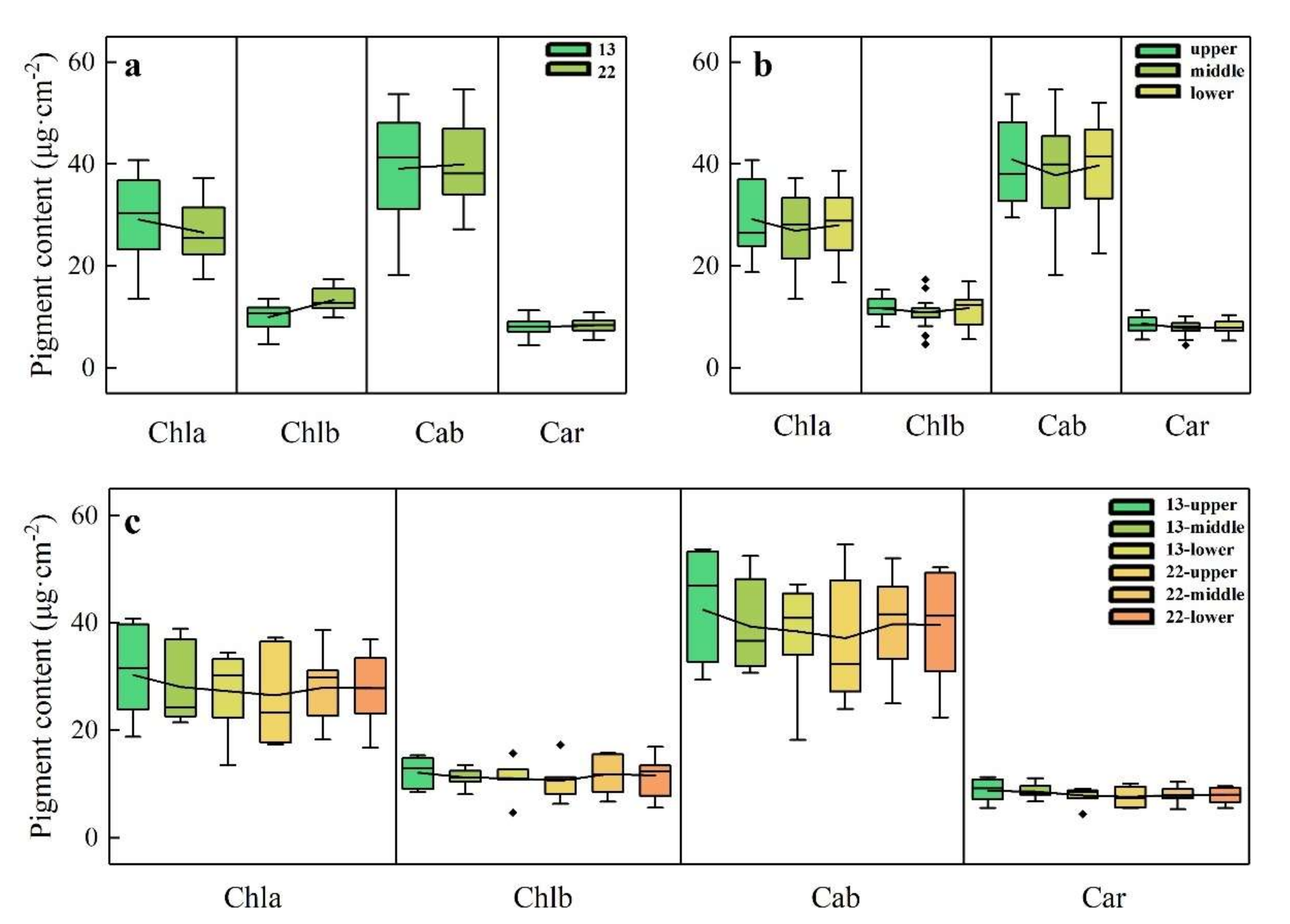
3.2. Statistical Distribution of Biochemical Pigments in Ginkgo Leaves

Figure 6 shows the box and whisker plots of the pigment content of Ginkgo leaves for different ages, heights, and their combinations. In terms of different ages (Figure 6a), except for Chla which showed a decreasing tendency with increase of age (decreased by 8.71%), Chlb (by 33.60%), Cab (by 2.1%) and Car (by 4.06%) were all increased. In terms of different height layers (Figure 6b), the vertical distribution patterns of different pigments were relatively consistent, with the highest content occurring in the upper vertical layer (7.41–12.20% higher than the middle layer; 3.18–8.00% higher than the lower layer), followed by the lower vertical layer, then the middle vertical layer. Particularly, in terms of the combinations between ages and heights (Figure 6c), the pigment content of the 13-year-old part samples generally increased with height, whereas the pigment content of the 22-year-old part samples generally decreased with height.

3.3. Pigment Estimation Performance Using LUT-Based-Inversion Mothod

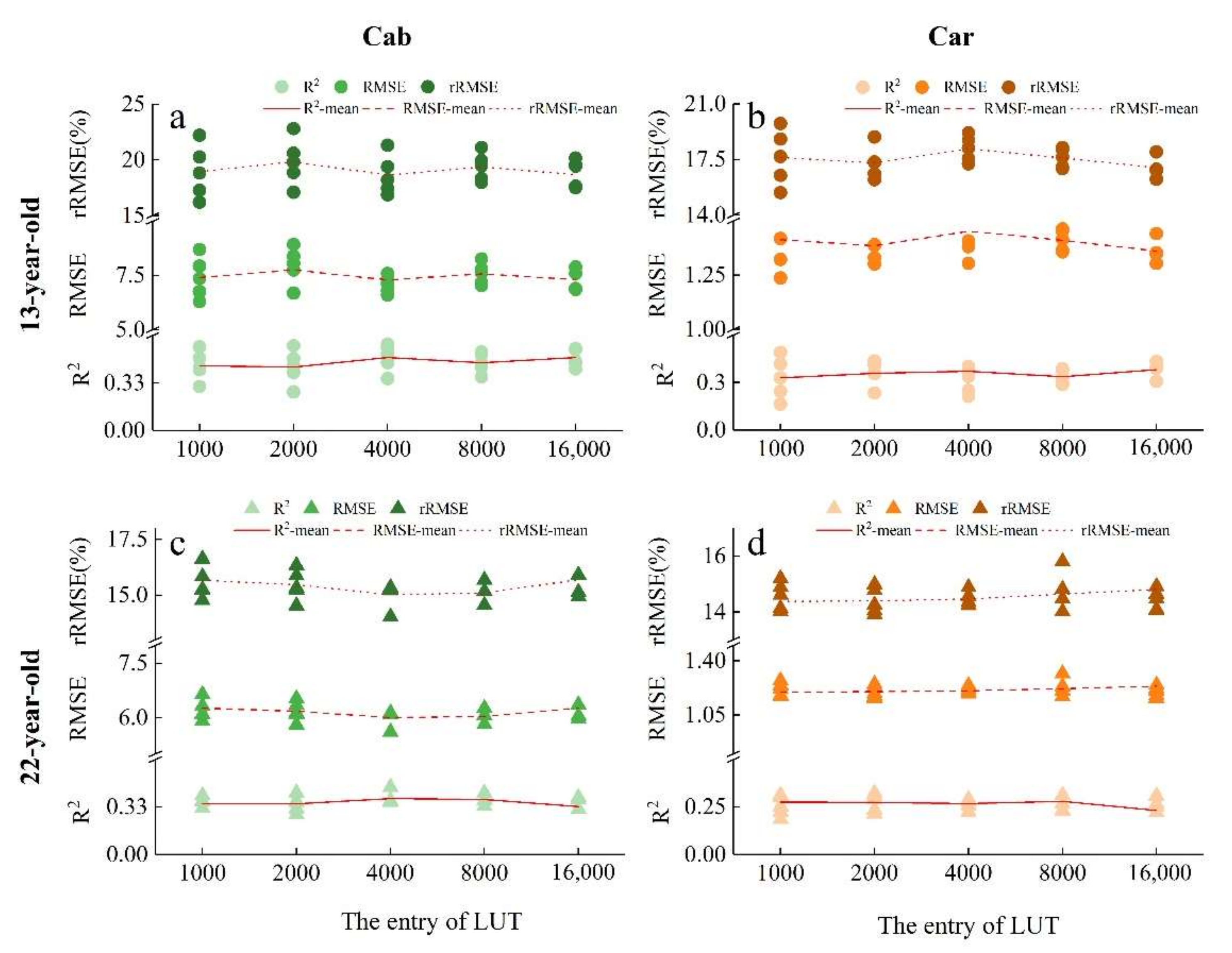
3.3.1. The Selection of Optimal LUT Entries for Estimating Cab and Car

The estimation accuracies of Cab and Car content using LUT-database-1 (50 LUTs) are shown in Figure 7. Compared with the RMSE function, the Cressie-Read function had better retrieval performance for Cab and Car content.
Regarding the estimation of Cab content, the pigment estimation accuracies for 13-year-old (R2 = 0.27–0.60, RMSE = 6.60–8.93 μg·cm−2, rRMSE = 16.86–22.81%) (Figure 7a) were higher than those for 22-year-old (R2 = 0.27–0.47, RMSE = 5.57–6.56 μg·cm−2, rRMSE = 13.94–16.44%) (Figure 7c). Additionally, regarding the Car content inversion, the pigment inversion accuracies for 13-year-old (R2 = 0.16–0.49, RMSE = 1.24–1.58 μg·cm−2, rRMSE = 15.42–19.78%) (Figure 7b) were slightly higher than or close to those of 22-year-old (R2 = 0.21–0.36, RMSE = 1.12–1.27 μg·cm−2, rRMSE = 13.46–15.20%) (Figure 7d). With the increase in the number entries of LUTs, the R2 for Cab and Car generally showed a tendency to increase from 1000 to 4000, and then decrease or keep stable from 4000 to 16,000, with more concentrated scatter points for five random repetitions. Therefore, this paper used a LUT with 4000 entries, which had a relatively high R2 and a relatively small RMSE, combined with the Cressie-Read cost function for subsequent pigments’ inversion.

3.3.2. The Selection of Specific Optimal LUTs for Estimating Cab and Car

The horizontal and vertical distributions mapping of pigments within Ginkgo canopies from two strips (i.e., of 13-year-old and 22-year-old plantations) are shown in Figure 8. The results of the best-performing LUT for estimating Cab (R2 = 0.60 for 13-year-old trees; R2 = 0.49 for 22-year-old trees) and Car (R2 = 0.46 for 13-year-old trees; R2 = 0.36 for 22-year-old trees) are shown in Figure 8(a1–d1).
The horizontal and vertical distributions of pigments for two strips are shown in Figure 8(a2–d2). The spatial distribution of Cab content and Car content within canopies exhibited similar patterns (Figure 8). In the horizontal direction, the pigment content of 13-year-old and 22-year-old ginkgo increased from inside the canopy to outside. In contrast, in the vertical direction, pigment content generally decreased along with the increase in the tree heights (Figure 8(a2–d2)).
Figure 9 shows the stacked histogram of Cab and Car estimations for different heights from the plots in Figure 8. Cab and Car content of the 22-year-old plots were generally higher than those of the 13-year-old plots (Figure 9c), yielding an increase of 5.37–55.67% for Cab content and 3.37–42.88% for Car content at different height levels (Figure 9a,b). The stacked histograms for 13-year-old trees showed that high frequency occurred at the middle range (32–52 μg·cm−2 for Cab; 5.8–9.8 μg·cm−2 for Car; Figure 9a,b). The stacked histograms for the 22-year-old trees showed that high frequency occurred at the high range (34–64 μg·cm−2 for Cab; 7.8–11.8 μg·cm−2 for Car; Figure 9a,b).

4. Discussion

In this paper, Cab and Car content of ginkgo canopies were well estimated using the LUT-based-inversion approach and fused multi-scale remote sensing data (LiDAR and hyperspectral images). To our best knowledge, this is the first attempt to map the 3D distribution of pigment content within tree canopies by the synthetic use of the PROSAIL model and fused hyperspectral cloud points.

4.1. Performance of LUT-Based-Inversion in Estimating Pigment Content

For the estimation of pigment content, the LUT-based-inversion approach (R2 = 0.36–0.60, Figure 8(a1–d1)) performed better than SI models (R2 = 0.25–0.46, Supplementary Figure S3). In particular, the LUT-based-inversion approach can further improve inversion accuracy when applying the optimal entry size of 4000 for two ages with the Cressie-Read cost function (Figure 7). This can be explained by the fact that the PROSAIL model was developed based on radiative transfer principles, which help improve its universality and applicability in biochemical and biophysical estimations for multiple vegetation species and growth environments. Therefore, the LUT-based-inversion approach has a more robust estimation performance for pigments, which can be effectively used to determine the distribution of pigments within Gingko canopies of individual trees or forests.
Despite lower absorption features of Car than Cab, extracting the Car content by adopting the Cab–Car relationship might also lead to bias (overestimation for samples of Car < 6 μg/cm2; underestimation for samples of Car > 10 μg/cm2) in the worse performance of Car inversion (R2 = 0.46–0.36, Figure 8(b1,d1)) to some extent, as compared to the Cab estimation (R2 = 0.60–0.49, Figure 8(a1,c1)).

4.2. Potential for Mapping Pigments Content Based on Hyperspectral Fusion Point Cloud Coupling with PROSAIL Model

Numerous studies have proved that the combination of the PROSAIL model and hyperspectral data has the capability to estimate biochemical traits [43,65]. Different from previous studies which usually mapped the horizontal distribution of pigments only, this study was successful in coupling hyperspectral fusion point clouds with the PROSAIL model for mapping horizontal and vertical distribution of pigments. Specifically, based on the fusion remote sensing data, the LUT-based-inversion approach derived from the PROSAIL model achieved relatively preferable accuracies (R2 = 0.36–0.60, Figure 8(a1–d1)) for mapping the 3D distribution of pigments [65].
Additionally, the analysis results of pigment distribution (Figure 9) exhibited that the lower canopy had higher pigment content to some extent. This suggests that some uncertainties occurred when estimating pigments of total canopies using the upper canopy samples only. Thus, coupling the fused remote sensing data and PROSAIL model provides a promising approach for accurately mapping the 3D distribution of pigments.

4.3. Factors Affecting Pigment Distribution on Canopy Surfaces

In this study, the effects of age, light and canopy structure on pigment content and their distribution within forest canopies were analyzed.
In terms of age, with the growth of age, the tree growth curve presents an ‘S’ shaped growth process (i.e., slow–fast–slow) [9]. Therefore, the growth potential and photosynthetic capacity for ages 13-year-old and 22-year-old are different. The results showed that Cab and Car content of 22-year-old Ginkgo trees (middle stand age) was higher than that of 13-year-old (young-aged) (Figure 6 and Figure 8). This may be attributed to the fact that 22-year-old Ginkgo trees are in the middle-aged growth stage, with stronger photosynthesis and more Cab accumulated in leaves.
In terms of light conditions, the content and distribution of Cab and Car in leaves are affected by light conditions, leading to variation in the strength of photosynthetic capacity of leaves [66]. In the horizontal direction, outer canopies received more direct solar radiation than the internal canopies, while the internal canopies are dominated by diffuse radiation [67]. This could be the main reason for the fact that the pigment content increases from inside the canopies to outside.
In terms of the canopy structure, the differences in LAI between various vertical layers may result in shadow effects to a different extent [68,69]. Additionally, the height and vertical position of leaves in the crown are important factors, which affect the pigment content and photosynthetic capacity [70]. The middle canopies have higher pigment content than upper and lower layers. This can be attributed to differences in the leaf expansion and senescence processes between the three height layers. Compared to middle layers, with the expansion of young leaves yielding higher photosynthetic capacity, young leaves might grow and wait for spreading out from the top canopies. In contrast, the leaves of the lower layers can be faster in the senescence process with decreased photosynthetic capacity compared to the other two height layers. Meanwhile, the maximum crown width mainly depends on the middle and lower canopy, resulting in a larger leaf area ratio and a wider light-receiving area in the middle and lower canopy, thus yielding higher content of Cab and other pigments synthesized in leaves. Moreover, the middle and lower leaves of the canopy may accumulate more Cab to obtain more light energy for alleviation of the impact of shadow effects [71,72].
Moreover, light and canopy structures have interaction influences with each other. However, it is complicated to quantify their respective effects on pigment estimation. We found that the estimated results from point-based reflectance (Figure 8) showed inconsistent patterns with the measured data of sampling trees (Figure 6). This may be because the sampling trees and corresponding leaf samples are limited to some extent.
The change process for leaf biochemical pigments content is complex and continuous, comprehensively controlled and regulated by multiple factors to meet its growth needs. This paper indirectly proves that different height levels influence the pigment content of leaves. More importantly, the estimation of leaf biochemical traits using fused hyperspectral point clouds at different height levels can effectively improve 3D distribution information for pigments within canopies, which is consistent with most previous research results [45,69].

4.4. Future Research and Application

Previous studies proved that RTM coupled with machine learning algorithms can partly improve inversion accuracies (mainly modeled with a mean R2 > 0.60 [73]). Thus, further studies may consider settings with machine learning algorithms (such as Gaussian processes regression) for estimation of pigments to improve accuracy. Furthermore, the PROSAIL model or other RTM can couple with the hyperspectral fusion point cloud to estimate the biochemical content of canopies in different regions, different tree species and different growth conditions in the future.

5. Conclusions

We attempted to perform multi-source remote sensing data inversion estimation in the PROSAIL model for biochemical pigments of Ginkgo, and fused hyperspectral imagery with LiDAR data to obtain the fused hyperspectral point clouds, which were put into the PROSAIL model to construct the exclusive LUT for Ginkgo. Following the LUT, we explored the 3D distribution of pigments within canopies and the regularities in the horizontal and vertical profiles of pigments with age and height. The fusion of multi-source remote sensing data provides a 3D visualization method for pigment estimation. The main results from this study are summarized as follows:
  • The special LUTs for Ginkgo plantations were constructed with higher estimation accuracies (R2 = 0.36–0.60, rRMSE = 13.53–16.86% for PROSAIL models, Figure 8 R2 = 0.25–0.46, rRMSE = 16.25–19.37% for VIs models, Supplementary Figure S3). Considering the computation work, we calibrated the parameters of PROSAIL and found the optimal LUT entry (i.e., 4000);
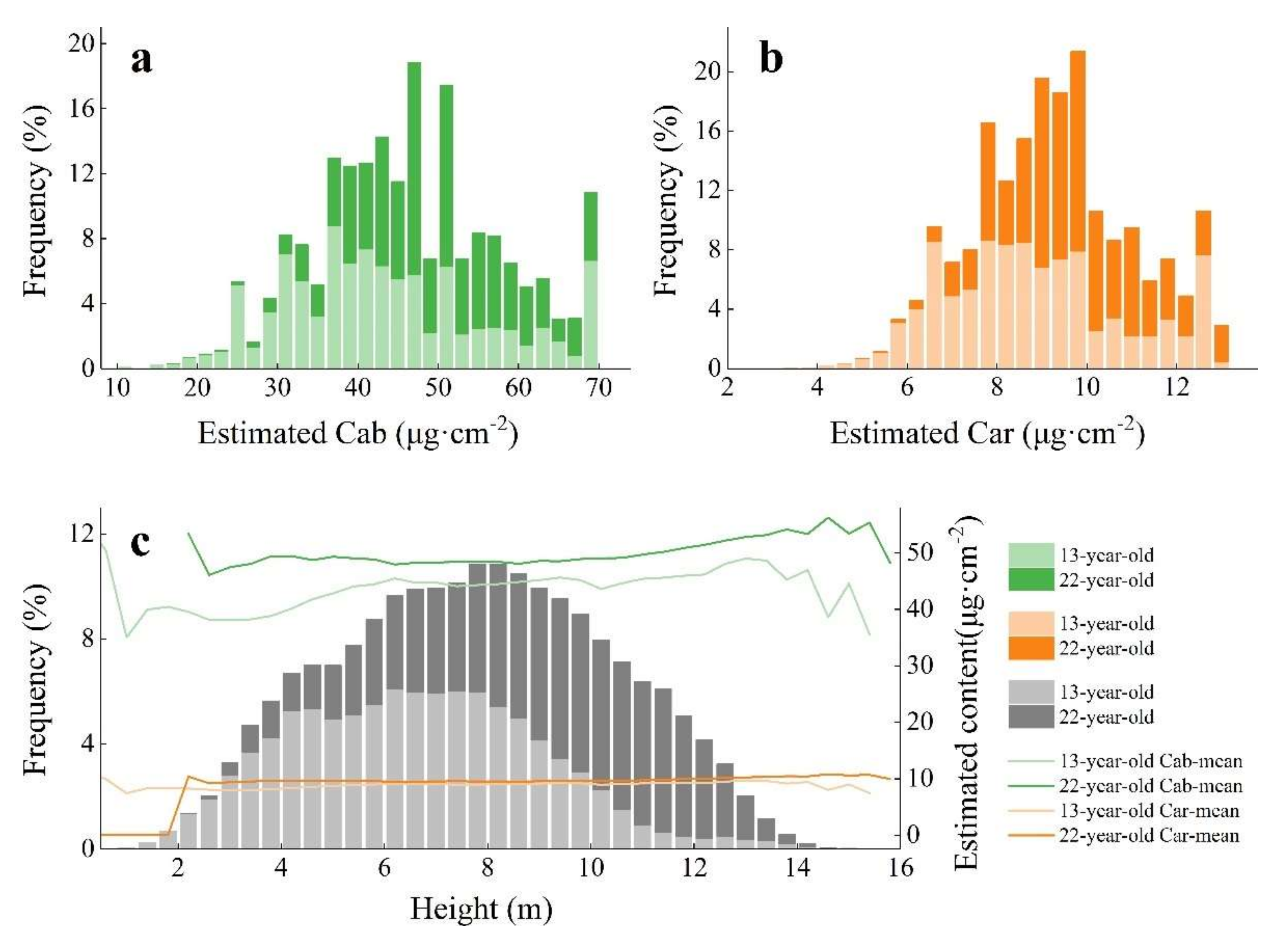
  • The pigment content of Ginkgo trees increased from inward to outward in the horizontal direction, but decreased along with increase in height in the vertical direction;
  • The hierarchical study in optimizing the inversion model once again emphasized its importance.

Supplementary Materials

The following supporting information can be downloaded at: https://www.mdpi.com/article/10.3390/rs14030715/s1. They can be found at the Supplementary Materials. Table S1. Summary of flight parameters and UAV-LiDAR and UAV-hyperspectral sensor properties. Figure S1. Comparison of the maximum-minimum value, mean value and mean ± standard deviation of the measured reflectance spectra of the 42 part samples (six parts for seven individual sampling trees). (a): the comparison of the total 42 part samples; (b): the comparison of the 13-year-old part samples; (c): the comparison of the 22-year-old part samples; (d): the comparison of the upper part samples; (e): the comparison of the middle part samples; (f): the comparison of the lower part samples. Figure S2. The pixel-based and point-based maximum-minimum, mean, and mean ± standard deviation reflectance curves for each of the two ages with six part samples. (a1,b1): the hyperspectral images of sampling tree for13-year-old and 22-year-old, respectively (the red, green and blue line represent the boundary of the upper, the middle, the lower layer); (a2–a7): the result of 13-year-old part samples; (b2–b7): the result of 22-year-old part samples; Note: the “2-7” of alphabetical tab represent the results of the six part samples (i.e., upper north, upper south, middle north, middle south, lower north and lower south); the “pixel-max, pixel-min, pixel-mean” of Figure represent the curve of the max reflectance value, the min reflectance value and the mean reflectance value for the pixel-based, respectively; “point-min, point-min, point-mean” of Figure represent the curve of the max reflectance value, the min reflectance value and the mean reflectance value for the point-based, respectively. Figure S3. Relationship between measured and estimated pigments content based on four types SI models. (a–d): the result of Cab; (e–h): the result of Car; (a,e): the result of SR index; (b,f): the result of mSR index; (c,g): the result of ND index; (d,h): the result of SR index. Note: Cab = total chlorophyll content (μg·cm−2); Car = total carotenoids content (μg·cm−2); SR = the simple ratio index; mSR = the modified simple ratio index; ND = the normalized difference index; DD = the double difference index.

Author Contributions

S.Y. wrote the original manuscript; S.Y. and K.Z. performed the experiments; S.Y. and K.Z. analyzed the data; L.C. conceived and designed the experiments; X.S. provided analysis tools and codes; S.Y., K.Z., L.C. edited the manuscript. All authors have read and agreed to the published version of the manuscript.

Funding

National Natural Science Foundation of China (31922055, 31770590), and the Priority Academic Program Development of Jiangsu Higher Education Institutions (PAPD).

Acknowledgments

The authors gratefully acknowledge the foresters in Dongtai Forest for their assistance with data collection and sharing their experiences of the local forests. We also would like to thank the graduate students from the department of forest management and silviculture at Nanjing Forestry University for helping in data collection and providing suggestions for improving this study.

Conflicts of Interest

The authors declare no conflict of interest.

References

  1. Brockerhoff, E.G.; Jactel, H.; Parrotta, J.A.; Quine, C.P.; Sayer, J. Plantation forests and biodiversity: Oxymoron or opportunity? Biodivers. Conserv. 2008, 17, 925–951. [Google Scholar] [CrossRef]
  2. National Forestry and Grassland Administration. China Forest Resources Report 2009–2013; China Forestry Publishing House: Beijing, China, 2014. [Google Scholar]
  3. Yan-Long, W.; Xiao-Yu, C.H.E.; Yu-Guang, L.I.U.; Ya-Nan, L.I.; Yan-Hui, L.I. Study on the changes of leaf color parameter and pigment content of Ginkgo biloba leaf in autumn. J. Hebei Agric. Univ. 2015, 38, 28–32. [Google Scholar]
  4. Yanling, N.; Zhao, Y. Study on Inversion of Vegetation Biochemical Parameters through Hyperspectral Data; Northeast Normal University: Changchun, China, 2010. [Google Scholar]
  5. Gara, T.W.; Darvishzadeh, R.; Skidmore, A.K.; Tiejun, W.; Heurich, M. Evaluating the performance of PROSPECT in the retrieval of leaf traits across canopy throughout the growing season. Int. J. Appl. Earth Obs. Geoinf. 2019, 83, 101919. [Google Scholar] [CrossRef]
  6. Jagodziński, A.M.; Dyderski, M.K.; Rawlik, K.; Katna, B. Seasonal variability of biomass, total leaf area and specific leaf area of forest understory herbs reflects their life strategies. For. Ecol. Manag. 2016, 374, 71–81. [Google Scholar] [CrossRef]
  7. Meng, W.; Xidong, W. Effects of Planting Densities and Spatial Distribution Patterns on Canopy Structure and Physiological Characters of Summer Maize; Tianjin Agricultural University: Tianjin, China, 2016. [Google Scholar]
  8. Sellin, A.; Kupper, P. Effects of light availability versus hydraulic constraints on stomatal responses within a crown of silver birch. Oecologia 2005, 142, 388–397. [Google Scholar] [CrossRef] [PubMed]
  9. Xiao-Fu, W.; Yue-Li, H. Study of the Dynamics Models of Forest Growth and Nutrition Ⅷ Diameter Age and Growth Parameter Determination. J. Cent. South For. Univ. 2001, 21, 1–5. [Google Scholar]
  10. Clevers, J.G.P.W.; Kooistra, L. Using hyperspectral remote sensing data for retrieving canopy chlorophyll and nitrogen content. IEEE J. Sel. Top. Appl. Earth Obs. Remote Sens. 2012, 5, 574–583. [Google Scholar] [CrossRef]
  11. Paź-Dyderska, S.; Dyderski, M.K.; Nowak, K.; Jagodziński, A.M. On the sunny side of the crown-quantification of intra-canopy SLA variation among 179 taxa. For. Ecol. Manag. 2020, 472, 118254. [Google Scholar] [CrossRef]
  12. Dong-Yan, X. Application Status and Prospects of Remote Sensing in Forestry. Sci. Technol. Vis. 2014, 21, 309–311. [Google Scholar] [CrossRef]
  13. Qingwang, L.; Bingxiang, T.; Kailong, H.; Xue, F.; Zengyuan, L.; Yong, P.; Shiming, L. The remote sensing experiment on airborne LiDAR and hyperspectral integrated system for subtropical forest estimation. Chin. High Technol. Lett. 2016, 26, 264–274. [Google Scholar] [CrossRef]
  14. Fu, X.; Zhang, Z.; Cao, L.; Coops, N.C.; Goodbody, T.R.H.; Liu, H.; Shen, X.; Wu, X. Assessment of approaches for monitoring forest structure dynamics using bi-temporal digital aerial photogrammetry point clouds. Remote Sens. Environ. 2021, 255, 112300. [Google Scholar] [CrossRef]
  15. Qinghua, G.; Jin, L.; Shengli, T.; Baolin, X.; Le, L.; Guangcai, X.; Wenkai1, L.; Fangfang, W.; Yumei, L.; Linhai, C.; et al. Perspectives and prospects of LiDAR in forest ecosystem monitoring and modeling. Chin. Sci. Bull 2014, 59, 459–478. (in Chinese). [Google Scholar] [CrossRef]
  16. Kai, Z.; Lin, C. The status and prospects of remote sensing applications in precision silviculture. J. Remote Sens. 2021, 25, 423–438. [Google Scholar] [CrossRef]
  17. Li-Juan, C.; Lin, S.; Yan-Juan, Y.; Yan, S. Research Developments on Inversion of Vegetation Biochemistry Compositions by Quantitative Remote Sensing. J. Atmos. Environ. Opt. 2011, 6, 163–178. [Google Scholar] [CrossRef]
  18. Yanfang, X.; Demin, Z.; Wenji, Z. Review of inversing biophysical and biochemical vegetation parameters in various spatial scales using radiative transfer models. J. Remote Sens. 2013, 33, 3291–3297. [Google Scholar] [CrossRef]
  19. De-Hua, Z.; Jian-Long, L.; Zi-Jian, S. Hyperspectral Remote Sensing for Estimating Biochemical Variables of Canopy. Adv. Earth Sci. 2003, 18, 94–99. [Google Scholar] [CrossRef]
  20. Changshan, W.; Qingx, T.; Lanfen, Z.; Weidong, L. Correlation Analysis Between Spectral Data and Chlorophyll of Rice and Maize. J. Basic Sci. Eng. 2002, 6, 1–5. [Google Scholar] [CrossRef]
  21. Jacquemoud, S.; Baret, F. PROSPECT: A model of leaf optical properties spectra. Remote Sens. Environ. 1990, 34, 75–91. [Google Scholar] [CrossRef]
  22. Jacquemoud, S.; Ustin, S.L.; Verdebout, J.; Schmuck, G.; Andreoli, G.; Hosgood, B. Estimating leaf biochemistry using the PROSPECT leaf optical properties model. Remote Sens. Environ. 1996, 56, 194–202. [Google Scholar] [CrossRef]
  23. Baret, F.; Fourty, T. Estimation of leaf water content and specific leaf weight from reflectance and transmittance measurements. Agronomie 1997, 17, 455–464. [Google Scholar] [CrossRef] [Green Version]
  24. Feret, J.B.; François, C.; Asner, G.P.; Gitelson, A.A.; Martin, R.E.; Bidel, L.P.R.; Ustin, S.L.; le Maire, G.; Jacquemoud, S. PROSPECT-4 and 5: Advances in the leaf optical properties model separating photosynthetic pigments. Remote Sens. Environ. 2008, 112, 3030–3043. [Google Scholar] [CrossRef]
  25. Barry, K.M.; Newnham, G.J.; Stone, C. Estimation of chlorophyll content in Eucalyptus globulus foliage with the leaf reflectance model PROSPECT. Agric. For. Meteorol. 2009, 149, 1209–1213. [Google Scholar] [CrossRef]
  26. Féret, J.-B.; François, C.; Gitelson, A.; Asner, G.P.; Barry, K.M.; Panigada, C.; Richardson, A.D.; Jacquemoud, S. Optimizing spectral indices and chemometric analysis of leaf chemical properties using radiative transfer modeling. Remote Sens. Environ. 2011, 115, 2742–2750. [Google Scholar] [CrossRef] [Green Version]
  27. Féret, J.-B.; Gitelson, A.A.; Noble, S.D.; Jacquemoud, S. PROSPECT-D: Towards modeling leaf optical properties through a complete lifecycle. Remote Sens. Environ. 2017, 193, 204–215. [Google Scholar] [CrossRef] [Green Version]
  28. Verhoef, W. Light scattering by leaf layers with application to canopy reflectance modeling: The SAIL model. Remote Sens. Environ. 1984, 16, 125–141. [Google Scholar] [CrossRef] [Green Version]
  29. Kuusk, A.; Nilson, T. A Directional Multispectral Forest Reflectance Model. Remote Sens. Environ. 2000, 72, 244–252. [Google Scholar] [CrossRef]
  30. Demarez, V.; Gastellu-Etchegorry, J.P. A Modeling Approach for Studying Forest Chlorophyll Content. Remote Sens. Environ. 2000, 71, 226–238. [Google Scholar] [CrossRef]
  31. Goel, N.S.; Thompson, R.L. A snapshot of canopy reflectance models and a universal model for the radiation regime. Remote Sens. Rev. 2000, 18, 197–225. [Google Scholar] [CrossRef]
  32. Verhoef, W.; Bach, H. Simulation of hyperspectral and directional radiance images using coupled biophysical and atmospheric radiative transfer models. Remote Sens. Environ. 2003, 87, 23–41. [Google Scholar] [CrossRef]
  33. Baret, F.; Jacquemoud, S.; Guyot, G.; Leprieur, C. Modeled analysis of the biophysical nature of spectral shifts and comparison with information content of broad bands. Remote Sens. Environ. 1992, 41, 133–142. [Google Scholar] [CrossRef]
  34. Dawson, T.P.; Curran, P.J.; North, P.R.J.; Plummer, S.E. The Propagation of Foliar Biochemical Absorption Features in Forest Canopy Reflectance: A Theoretical Analysis. Remote Sens. Environ. 1999, 67, 147–159. [Google Scholar] [CrossRef]
  35. Verhoef, W.; Bach, H. Remote sensing data assimilation using coupled radiative transfer models. Phys. Chem. Earth Parts A/B/C 2003, 28, 3–13. [Google Scholar] [CrossRef]
  36. Dash, J.; Curran, P.J. The MERIS terrestrial chlorophyll index. Int. J. Remote Sens. 2004, 25, 5403–5413. [Google Scholar] [CrossRef]
  37. Kötz, B.; Schaepman, M.; Morsdorf, F.; Bowyer, P.; Itten, K.; Allgöwer, B. Radiative transfer modeling within a heterogeneous canopy for estimation of forest fire fuel properties. Remote Sens. Environ. 2004, 92, 332–344. [Google Scholar] [CrossRef]
  38. Zarco-Tejada, P.J.; Miller, J.R.; Harron, J.; Hu, B.; Noland, T.L.; Goel, N.; Mohammed, G.H.; Sampson, P. Needle chlorophyll content estimation through model inversion using hyperspectral data from boreal conifer forest canopies. Remote Sens. Environ. 2004, 89, 189–199. [Google Scholar] [CrossRef]
  39. Verhoef, W.; Jia, L.; Xiao, Q.; Su, Z. Unified Optical-Thermal Four-Stream Radiative Transfer Theory for Homogeneous Vegetation Canopies. IEEE Trans. Geosci. Remote Sens. 2007, 45, 1808–1822. [Google Scholar] [CrossRef]
  40. Dong, L.; Tao, C.; Min, J.; Kai, Z.; Ning, L.; Xia, Y.; Yongchao, T.; Yan, Z.; Weixing, C. PROCWT: Coupling PROSPECT with continuous wavelet transform to improve the retrieval of foliar chemistry from leaf bidirectional reflectance spectra. Remote Sens. Environ. 2018, 206, 1–14. [Google Scholar] [CrossRef]
  41. Berger, K.; Wang, Z.; Danner, M.; Wocher, M.; Mauser, W.; Hank, T. Simulation of Spaceborne Hyperspectral Remote Sensing to Assist Crop Nitrogen Content Monitoring in Agricultural Crops. In Proceedings of the IEEE International Geoscience and Remote Sensing Symposium, Valencia, Spain, 22–27 July 2018; Volume 2018, pp. 3801–3804. [Google Scholar]
  42. Féret, J.-B.; le Maire, G.; Jay, S.; Berveiller, D.; Bendoula, R.; Hmimina, G.; Cheraiet, A.; Oliveira, J.C.; Ponzoni, F.J.; Solanki, T.; et al. Estimating leaf mass per area and equivalent water thickness based on leaf optical properties: Potential and limitations of physical modeling and machine learning. Remote Sens. Environ. 2019, 231, 110959. [Google Scholar] [CrossRef]
  43. Duan, S.-B.; Li, Z.-L.; Wu, H.; Tang, B.-H.; Ma, L.; Zhao, E.; Li, C. Inversion of the PROSAIL model to estimate leaf area index of maize, potato, and sunflower fields from unmanned aerial vehicle hyperspectral data. Int. J. Appl. Earth Obs. Geoinf. 2014, 26, 12–20. [Google Scholar] [CrossRef]
  44. Zhiqing, C.; Jinsong, Z. Estimation Model of Poplar Plantation Productivity with Hyperspectral Information and Remote Sensing; Chinese Academy of Forestry: Beijing, China, 2015. [Google Scholar]
  45. Xin, S.; Lin, C.; Coops, N.C.; Hongchao, F.; Xiangqian, W.; Hao, L.; Guibin, W.; Fuliang, C. Quantifying vertical profiles of biochemical traits for forest plantation species using advanced remote sensing approaches. Remote Sens. Environ. 2020, 250, 112041. [Google Scholar] [CrossRef]
  46. Lichtenthaler, H.K.; Wellburn, A.R. Determinations of total carotenoids and chlorophylls a and b of leaf extracts in different solvents. Biochem. Soc. Trans. 1983, 11, 591–592. [Google Scholar] [CrossRef] [Green Version]
  47. Savitzky, A.; Golay, M.J.E. Smoothing and Differentiation of Data by Simplified Least Squares Procedures. Anal. Chem. 1964, 36, 1627–1639. [Google Scholar] [CrossRef]
  48. Wen-Ting, Q.; Hui, Z.; Hong-Mei, L.; Wan-Juan, Y.; Hua-Long, L. Remote Recognition and Growth Monitoring of Winter Wheat in Key Stages Based on S-G Filter in Guanzhong Region. Chin. J. Agrometeorol. 2015, 36, 93–99. [Google Scholar]
  49. Morsdorf, F.; Kötz, B.; Meier, E.; Itten, K.I.; Allgöwer, B. Estimation of LAI and fractional cover from small footprint airborne laser scanning data based on gap fraction. Remote Sens. Environ. 2006, 104, 50–61. [Google Scholar] [CrossRef]
  50. Coops, N.C.; Hilker, T.; Wulder, M.A.; St-Onge, B.; Newnham, G.; Siggins, A.; Trofymow, J.A. (Tony) Estimating canopy structure of Douglas-fir forest stands from discrete-return LiDAR. Trees 2007, 21, 295–310. [Google Scholar] [CrossRef] [Green Version]
  51. Næsset, E.; Bjerknes, K.-O. Estimating tree heights and number of stems in young forest stands using airborne laser scanner data. Remote Sens. Environ. 2001, 78, 328–340. [Google Scholar] [CrossRef]
  52. Lovell, J.L.; Jupp, D.L.B.; Culvenor, D.S.; Coops, N.C. Using airborne and ground-based ranging lidar to measure canopy structure in Australian forests. Can. J. Remote Sens. 2003, 29, 607–622. [Google Scholar] [CrossRef]
  53. Xi-Guang, Y.; Wen-Yi, F.; Ying, Y. Estimation of Forest Canopy Chlorophyll Content Based on PROSPECT and SAIL models. Spectrosc. Spectr. Anal. 2010, 30, 3022–3026. [Google Scholar] [CrossRef]
  54. Bowyer, P.; Danson, F.M. Sensitivity of spectral reflectance to variation in live fuel moisture content at leaf and canopy level. Remote Sens. Environ. 2004, 92, 297–308. [Google Scholar] [CrossRef]
  55. Keenan, T.F.; Niinemets, Ü. Global leaf trait estimates biased due to plasticity in the shade. Nat. Plants 2016, 3, 16201. [Google Scholar] [CrossRef] [Green Version]
  56. Junhua, Z.; Jiabao, Z. Response of the Spectral Reflectance to Different Pigments of Summer Maize. Acta Agric. Boreali-Occident. Sin. 2010, 19, 70–76. [Google Scholar]
  57. La, Q.; Chun-Jiang, Z.; Wen-Jiang, H.; Han-Hai, L. Sensitivity Analysis of Canopy Spectra to Canopy Structural Parameters Based on Multi-temporal Data. Geogr. Geo-Inf. Sci. 2009, 25, 17–25. [Google Scholar]
  58. Zongjian, Z.; Yuyan, L.; Mingchun, G. Study on the Canopy Structure and Photosynthetic Characteristics of Ginkgo Biloba L.Saplings; Hebei Normal University of Science and Technology: Qin Huang Dao Shi, China, 2014. [Google Scholar]
  59. Xiangqian, W.; Lin, C.; Xin, S.; Guibin, W.; Fuliang, C. Estimation of Effective Leaf Area Index Using UAV-Based LiDAR in Ginkgo Plantations. For. Resour. Manag. 2020, 56, 74–86. [Google Scholar]
  60. Dong, L.; Jing, M.C.; Xiao, Z.; Yan, Y.; Jie, Z.; Hengbiao, Z.; Kai, Z.; Xia, Y.; Yongchao, T.; Yan, Z.; et al. Improved estimation of leaf chlorophyll content of row crops from canopy reflectance spectra through minimizing canopy structural effects and optimizing off-noon observation time. Remote Sens. Environ. 2020, 248, 111985. [Google Scholar] [CrossRef]
  61. Cheng-Yan, G.; Hua-Qiang, D.; Guo-Mo, Z.; Ning, H.; Xiao-Jun, X.; Xiao, Z.; Xiao-Yan, S. Retrieval of leaf area index of Moso bamboo forest with Landsat Thematic Mapper image based on PR OSAIL canopy radiative transfer model. Chin. J. Appl. Ecol. 2013, 24, 2248–2256. [Google Scholar]
  62. Sinha, S.K.; Padalia, H.; Dasgupta, A.; Verrelst, J.; Rivera, J.P. Estimation of leaf area index using PROSAIL based LUT inversion, MLRA-GPR and empirical models: Case study of tropical deciduous forest plantation, North India. Int. J. Appl. Earth Obs. Geoinf. 2020, 86, 102027. [Google Scholar] [CrossRef]
  63. Zhenhai, L.; Zhenhong, L.; Fairbairn, D.; Na, L.; Bo, X.; Haikuan, F.; Guijun, Y. Multi-LUTs method for canopy nitrogen density estimation in winter wheat by field and UAV hyperspectral. Comput. Electron. Agric. 2019, 162, 174–182. [Google Scholar] [CrossRef]
  64. Verrelst, J.; Romijn, E.; Kooistra, L. Mapping Vegetation Density in a Heterogeneous River Floodplain Ecosystem Using Pointable CHRIS/PROBA Data. Remote Sens. 2012, 4, 2866–2889. [Google Scholar] [CrossRef] [Green Version]
  65. Verrelst, J.; Muñoz, J.; Alonso, L.; Delegido, J.; Rivera, J.P.; Camps-Valls, G.; Moreno, J. Machine learning regression algorithms for biophysical parameter retrieval: Opportunities for Sentinel-2 and -3. Remote Sens. Environ. 2012, 118, 127–139. [Google Scholar] [CrossRef]
  66. Chun-Xia, H.; Ji-Yue, L.; Yan-Xiang, Z.; Quan-Shui, Z.; Xie, B.; Yi-Ting, D. Differences in leaf mass per area, photosynthetic pigments and δ13C by orientation and crown position in five greening tree species. Chin. J. Plant Ecol. 2010, 34, 134–143. [Google Scholar] [CrossRef]
  67. Feng-Li, H.; Fei, W.; Qin-Ping, W.; Xiao-Wei, W.; Qiang, Z. Relationship Between Distribution of Relative Light Intensity in Canopy and Yield and Quality of Peach Fruit. Sci. Agric. Sin. 2008, 41, 502–507. [Google Scholar]
  68. Shaoxuan, L.; Fuliang, C. Study of Crown Structure Feacture in the Timber Ginkgo; Nanjing Forestry University: Nanjing, China, 2014. [Google Scholar]
  69. Yong, L.; Hairong, H.; Fengfeng, K.; Xiaoqin, C.; Ke, L.; Bin, Z.; Yali, S. Spatial Heterogeneity of Photosynthetic Characterisitics of Pinus tabulaeformis Canopy. J. Northeast For. Univ. 2013, 41, 32–35. [Google Scholar]
  70. Xue-Hong, Z.; Qing-Jiu, T.; Run-Ping, S. Analysis of Directional Characteristics of Winter Wheat Canopy Spectra. Spectrosc. Spectr. Anal. 2010, 30, 1600–1605. [Google Scholar] [CrossRef]
  71. Ghosh, A.P.; Dass, A.; Krishnan, P.; Kaur, D.; Rana, K. Assessment of photosynthetically active radiation (PAR), photosynthetic rate (NPR), biomass and yield of two maize varieties under varied planting dates and nitrogen application. J. Environ. Biol. 2017, 38, 683–688. [Google Scholar] [CrossRef]
  72. Wei, L.; Kun-Fang, K. Effects of Drought Stress on Photosynthetic Characteristics and Chlorophyll Fluorescence Parameters in Seedlings of Terminthia paniculata Grown under Different Light level. Acta Bot. Boreali-Occident. Sin. 2006, 26, 266–275. [Google Scholar] [CrossRef]
  73. Feilhauer, H.; Asner, G.P.; Martin, R.E. Multi-method ensemble selection of spectral bands related to leaf biochemistry. Remote Sens. Environ. 2015, 164, 57–65. [Google Scholar] [CrossRef]
Figure 1. The location of UAV flight in the Dongtai Forest. (a): the Dongtai Forest study site in Jiangsu Province; (b): the locations of two UAV flight strips in the study site; (c): the 13-year-old stripe and No.1–4 sampling trees location; (d): the 22-year-old stripe and No.5–7 sampling trees location.
Remotesensing 14 00715 g001
Figure 2. An overview of the analysis workflow for assessing the content of ginkgo pigments. Note: “N, S” represent the north and south orientation; “upper, middle, lower” represent the upper, the middle, and the lower vertical layer; “2 age-groups” represent age 13-year-old and age 22-year-old; “5 entries” represent the number of LUT entries, varying from 1000 to 16,000 with the step of multiplying as 2 (i.e., 1000, 2000, 4000, 8000, 16,000); “5 random repeats” represent running random parameter sampling 5 times; “30 random repeats” represent running random parameter sampling 30 time; Cab = Chlorophyll; Car = Carotenoid; LAI = Leaf area index; ALA = Average leaf angle; N = Structural coefficient; Cw = Water content; Cm = Dry matter content.
Remotesensing 14 00715 g002
Figure 3. The UAV-LiDAR and UAV-hyperspectral systems used in the study. (a): UAV platform with LiDAR system; (b): UAV platform with hyperspectral system.
Remotesensing 14 00715 g003
Figure 4. The LSA results of PROSAIL parameters. (ah): the result of N, Cab, Car, LAI, ALA, hspot, psoil and skyl, respectively. Note: N = Structural coefficient; Cab = Total chlorophyll content (μg·cm−2); Car = Carotenoid content (μg·cm−2); LAI = Leaf area index (m2·m−2); ALA = Average leaf angle (°); hspot = Hotspot; psoil = Fraction of dry soil; skyl = Fraction of diffuse radiation (%).
Remotesensing 14 00715 g004
Figure 5. Point cloud visualization and cross-sectional structure diagram of seven sampling trees. (ag): No. 1–7 sampling trees; (ac): 22-year-old sampling trees; (dg): 13-year-old sampling trees; (a1g1): the front view of single wood point cloud; (a2g2): the top view of single wood point cloud; (a3g3): height profile of a single wood point cloud; (a4g4): FP profile fitting curve of single wood. Note: upper = upper vertical layer; middle = middle vertical layer; lower = lower vertical layer.
Remotesensing 14 00715 g005
Figure 6. Box and whisker plots of the measured biochemical pigments for 42-part samples. (a): Box and whisker plots of biochemical pigments at different ages (b): Box and whisker plots of biochemical pigments at different heights; (c): Box and whisker plots of biochemical pigments at different heights under different ages. Note: Chla = chlorophyll a content (μg·cm−2); Chlb = chlorophyll b content (μg·cm−2); Cab = total chlorophyll content (μg·cm−2); Car = carotenoids content (μg·cm−2); 13 = 13-year-old part samples; 22 = 22-year-old part samples; upper = upper vertical samples; middle = middle vertical layer; lower = lower vertical samples; 13-upper = 13-year-old upper samples; 13-middle = 13-year-old middle samples; 13-lower = 13-year-old lower samples; 22-upper = 22-year-old upper samples; 22-middle = 22-year-old middle samples; 22-lower = 22-year-old lower samples.
Remotesensing 14 00715 g006
Figure 7. Summary of Cressie-Read function estimating accuracy of Cab and Car content at different ages. (a,c): accuracy results of Cab content; (b,d): accuracy results of Car content; (a,b): accuracy results of 13-year-old part samples; (c,d): accuracy results of 22-year-old part samples. Each entry result of Cab and Car for two ages was repeated five times. Note: Cab = total chlorophyll content (μg·cm−2); Car = carotenoids’ content (μg·cm−2).
Remotesensing 14 00715 g007
Figure 8. Horizontal and vertical estimation distribution of pigments content at different ages based on the best LUT by point-based hyperspectral data. (a): Cab estimation results of the 13-year-old plot (μg·cm−2); (b): Car estimation results of the 13-year-old plot (μg·cm−2); (c): Cab estimation results of the 13-year-old plot (μg·cm−2); (d): Car estimation results of the 13-year-old plot (μg·cm−2); (a1d1): the corresponding optimal inversion models; (a2d2): represent the horizontal and the vertical (from top to bottom in each figure) estimation distribution of pigment content (the orange cross-section was segmented to show the vertical distribution).
Remotesensing 14 00715 g008
Figure 9. Stacked histogram of the estimated distribution of biochemical pigments at different ages. (a): stacking diagram of frequencies for the estimated Cab content; (b) stacking diagram of frequencies for the estimated Car content; (c): stacking diagram of frequencies for the tree height and the mean distribution of pigments. Note: Cab = total chlorophyll content (μg·cm−2); Car = total carotenoids content (μg·cm−2).
Remotesensing 14 00715 g009
Table 1. Summary of flight parameters and UAV-LiDAR and UAV-hyperspectral sensor properties.
ParametersUAS-Hyperspectral SystemUAS-LiDAR System
SensorsZK-VNIR-FPG480Velodyne Puck VLP-16
Data of acquisition17 Aug. 201918 Aug. 2019
Flight height (m)8080
Flight speed (m·s−1)4.86
Side overlap (%)>20100
Focal length (mm)16-
IFOV/Beam divergence (mrad)0.93
Spatial resolution/Footprint (cm)18.7517
FOV/Maximum scan angle (°)26± 30
Wavelength (nm)403–929903
Spectral sampling (nm)2.3-
Number of bands2261
Average point density (pts·m−2)-169
Table 2. PROSAIL parameter range of variation for the LSA.
Model ParametersVariable (Unit)RangeStep
Structural coefficientN (-)1.1–1.70.1
Total chlorophyll contentCab (μg·cm−2)10–7010
Carotenoid contentCar (μg·cm−2)0–152.5
Leaf area indexLAI (m2·m−2)0–30.5
Average leaf angleALA (°)0–9015
Hotspothspot0.1–0.40.05
Fraction of dry soilpsoil0.4–10.1
Fraction of diffuse radiationskyl (%)10–7010
Table 3. Summary of values or ranges for each input parameter of PROSAIL.
Parameters of PROSPECT-D Model
ParametersVariable (Unit)Rang (13-year-old)Rang (22-year-old)Reference
Structural coefficientN (-)Fixed at 1.4Fixed at 1.4[21]
Total chlorophyll contentCab (μg·cm−2)10–7010–70The measured data
Carotenoid contentCar (μg·cm−2)0–150–150.1512 × Cab + 2.1864
Water contentCw (g·cm−2)Fixed at 0.017Fixed at 0.017The mean of measured data
Dry matter contentCm (g·cm−2)Fixed at 0.009Fixed at 0.009The mean of measured data
Anthocyanin contentCanth (μg·cm−2)Fixed at 0.0Fixed at 0.0[60]
Brown pigment contentCbrown (-)Fixed at 0.0Fixed at 0.0[60]
Parameters of SAIL model
Parameters Variable (Unit)Rang (13-year-old)Rang (22-year-old)Reference
Leaf area indexLAI (m2·m−2)0.3–30.3–3[59]
Average leaf angleALA (°)Fixed at 45Fixed at 45[58]
HotspothspotFixed at 0.15Fixed at 0.15[61]
Fraction of dry soilpsoilFixed at 0.8Fixed at 0.8[62]
Fraction of diffuse radiationskyl (%)Fixed at 10Fixed at 10The LSA result
Viewing zenith angleVZA(°)Fixed at 0Fixed at 0The flight time
Solar zenith angleSZA (°)Fixed at 35.5Fixed at 67.5The flight time
Relative azimuth angle RAA(°)Fixed at 115.2Fixed at 88.1The flight time
Publisher’s Note: MDPI stays neutral with regard to jurisdictional claims in published maps and institutional affiliations.

