Drone-Based Characterization of Seagrass Habitats in the Tropical Waters of Zanzibar

Abstract

Unmanned automatic systems (UAS) are increasingly being applied as an alternative to more costly time-consuming traditional methods for mapping and monitoring marine shallow-water ecosystems. Here, we demonstrate the utility of combining aerial drones with in situ imagery to characterize the habitat conditions of nine shallow-water seagrass-dominated areas on Unguja Island, Zanzibar. We applied object-based image analysis and a maximum likelihood algorithm on the drone images to derive habitat cover maps and important seagrass habitat parameters: the habitat composition; the seagrass species; the horizontal- and depth-percent covers, and the seascape fragmentation. We mapped nine sites covering 724 ha, categorized into seagrasses (55%), bare sediment (31%), corals (9%), and macroalgae (5%). An average of six seagrass species were found, and 20% of the nine sites were categorized as “dense cover” (40–70%). We achieved high map accuracy for the habitat types (87%), seagrass (80%), and seagrass species (76%). In all nine sites, we observed clear decreases in the seagrass covers with depths ranging from 30% at 1–2 m, to 1.6% at a 4–5 m depth. The depth dependency varied significantly among the seagrass species. Areas associated with low seagrass cover also had a more fragmented distribution pattern, with scattered seagrass populations. The seagrass cover was correlated negatively (r² = 0.9, p < 0.01) with sea urchins. A multivariate analysis of the similarity (ANOSIM) of the biotic features, derived from the drone and in situ data, suggested that the nine sites could be organized into three significantly different coastal habitat types. This study demonstrates the high robustness of drones for characterizing complex seagrass habitat conditions in tropical waters. We recommend adopting drones, combined with in situ photos, for establishing a suite of important data relevant for marine ecosystem monitoring in the Western Indian Ocean (WIO).

1. Introduction

The Western Indian Ocean (WIO) region’s seagrass meadows are extensive along the intertidal and subtidal zones [1,2]. Seagrasses are vital components of nearshore shallow-water ecosystems, as nurseries for juvenile fish, and as hotspots for abundant invertebrates [3,4,5]. Seagrass habitats also function as feeding grounds for small pelagic species, such as grazers, sea turtles, and sea urchins, among others [6], and they support aquacultures as well [7,8]. Furthermore, the seagrass habitats are important blue carbon sinks [9,10], and they play a crucial role in wave dissipation, sediment stabilization, and the uptake and retainment of nutrients in coastal waters [11,12,13,14].

An accelerated decline in seagrasses is occurring worldwide [15,16], including in the WIO region [1,2,17]. Natural events, such as diseases, waves, storms, and grazing by herbivores, such as sea urchins, have been responsible for both large-scale and local losses of seagrasses [18,19]. Furthermore, human-mediated stress has become a serious cause of seagrass habitat loss [19], affecting seagrasses by altering the water quality through nutrient and sediment loading from runoff, sewage, dredging, and filling [19,20,21,22]. Activities such as net dredging, boat navigation, anchoring [23], mooring [24,25], and seaweed farming [26] directly disturb the structures of seagrass meadows and cause habitat fragmentation. Underlying this degradation is a rapidly growing coastal population associated with the overexploitation of shallow-water marine ecosystems [2,7,18], as well as an increase in coastal tourism developments through hotel investment and emerging new urban centers [27,28,29,30].

With this pressure, research into seagrass habitats has proliferated in terms of understanding the seagrass abundance and diversity [1,18,31,32,33]. Other studies investigate seagrass interactions with other ecosystems, such as coral reefs [3,7], fisheries [3,5,34], seaweed farms [6,35], and mangroves [5], and assess the threats facing them [1,2,19,21,27]. Notwithstanding all these studies, the knowledge on the spatial distribution of seagrasses across the seascape in the WIO region remains quite limited, and an understanding of both the spatial extent and the processes affecting tropical seagrasses requires further investigation [1,2].

The mapping of seagrasses in the region has mainly been performed with mid-resolution satellite imagery, such as Sentinel 2 [36]. Particularly, seagrass mapping in Zanzibar has only been attempted with Landsat 8 for Chwaka Bay, and IKONOS imagery for Chumbe island [31,32], providing useful, but rather disjointed, information in the two local areas. Such application is useful in large-scale mapping, but it is limited to capturing the very dynamic habitat features of the shallow-water environment [37,38]. The delineation of the patchiness of the meadows at the local scale and the species differentiation could be more tricky with these methods [37]. Therefore, a mapping approach with high resolution for shallow-water seascapes is important.

Furthermore, the knowledge of the spatial distribution of seagrass meadows in the WIO region [1,2] is important to characterizing and assessing the changes in the marine ecosystem health [39,40], which is a central component of marine ecosystem monitoring programs around the world [41,42]. Different measures of seagrass health are being applied to characterize seagrass habitats [24,43,44,45]. A typical characterization includes variables such as the habitat areal extent, the percent cover, the species composition, and the seascape properties of fragmentation. The ecological conditions on the epiphytic loadings, the desiccation effect, wasting diseases, and marine algae [6,24,44,46,47,48,49] are also part of seagrass health characterization. Given the high ecosystem value of seagrass meadows and the usefulness of these habitats for marine ecosystem health [43,46], establishing a reliable, rapid, and cost-effective mapping approach to aid seagrass monitoring programs is indispensable [50].

The drone technique potentially offers an effective approach for mapping seagrass biomes [50,51,52,53,54]. Yet, the efficacy of drone observations depends on the resolution, the choice of mapping days, and the availability of in situ data for calibration [50,52,55,56]. The experiences using drones [37,40,50,54,57,58,59] are quite limited in the tropical waters of the WIO, with most of the studies using satellite imagery [31,32,60,61,62]. Specifically, the drone-based applications to describe the diverse shallow-water habitats around Zanzibar have not yet been documented.

The analysis of multispectral and RGB imagery has witnessed multiple techniques—pixel-based [63,64] and object-based [52,65,66] image analyses with common algorithms applied, including machine learning approaches, such as random forest, support vector machine [67], and the maximum likelihood algorithm [32,52,68]. For the objective of this study, we used an object-based analysis with a maximum likelihood classifier.

The present study applied an integrated approach, with drone-based imagery and in situ techniques, with the overall aim of characterizing the nearshore seagrass-dominated habitats in the tropical waters of the Zanzibar WIO region. Specifically, we utilize drone imagery to: (i) Characterize the habitat conditions in terms of their cover (seagrasses, macroalgae, coral reef, sand) and the composition of the seagrass species. In addition, we: (ii) Analyze the patterns in the seagrass cover, in terms of their distribution with depth, levels of fragmentation, and relations with the epiphyte and sea urchin densities. Finally, we (iii) Combine all the acquired information to classify these nearshore sites and provide recommendations for the future monitoring and management of coastal habitats around Zanzibar.

2. Materials and Methods

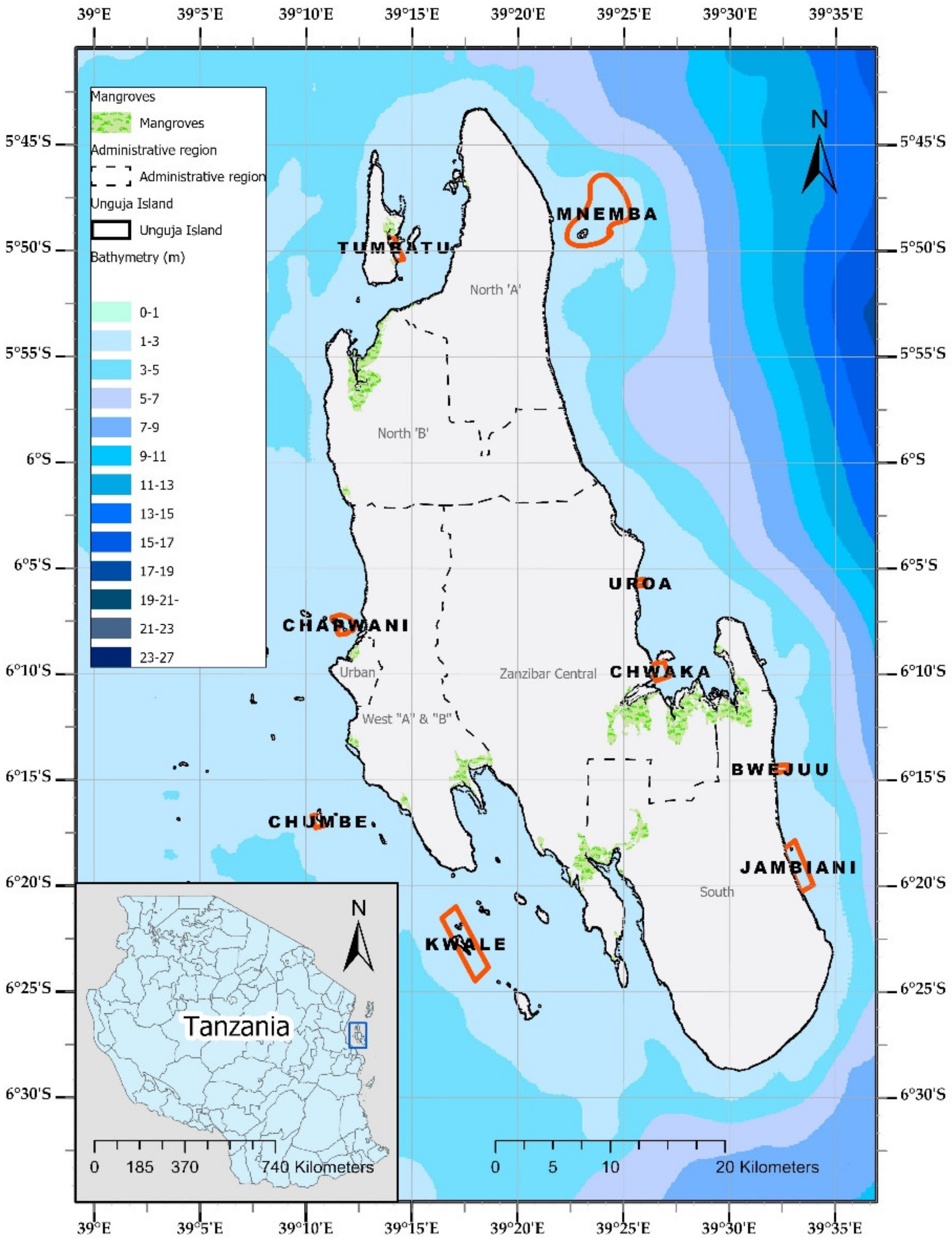
2.1. Study Design and Study Area Characteristics

We undertook mapping campaigns of the seagrass habitat conditions in nine nearshore areas within depth ranges of 1 to 10 m, using rotary drones and in situ observations. On the basis of these observations, we characterized the seagrass-dominated habitats with previously defined parameters: the habitat types, the species composition, the seascape properties, the sea urchin density epiphytic cover, and the dead leaves. These elements were integrated as part of the remote sensing of seagrass habitats and their health characterization [24,31,50,52,55,56,69,70,71,72,73]. We selected nine nearshore sites (Figure 1) on the basis of the available information on the distributions of the seagrasses, coral reefs, and macroalgal habitats. First, we highlighted sites with major seagrass cover by using classified Sentinel 2 imagery from June 2018, provided by DHI GRAS (Figure S1, Supplementary Material). Then, we chose study sites after a consideration of the level of the wave exposure and the coastal setting (mainland coast vs. islets). Finally, we applied preacquired local knowledge through reconnaissance surveys to fine-tune the most relevant mapping sites.

Zanzibar is a semiautonomous part of the United Republic of Tanzania, found in the Western Indian Ocean region, off the coast of eastern Africa. The archipelago consists of two major islands—Unguja (1670 km²) and Pemba (990 km²)—and about 50 small islets [28]. This study focuses on the largest island, Unguja (Figure 1). Unguja has a humid tropical monsoon climate, an average temperature of 27.5 °C, and receives bimodal rains [28]. The coastline of Unguja Island stretches for about 110 km, with a shoreline dominated by sandy beaches and mangroves. An extensive intertidal zone, varying up to 3 km, characterizes Zanzibar waters, which have distinctive semidiurnal tides, with the neap tide up to ca. 0.9 m, and the spring tide reaching heights of 3.2 m, whereas the tidal difference is more pronounced in the Zanzibar channel, ranging from 2.7 m to 4.2 m [28].

The nine selected study sites represent areas where the seagrass habitats cover extensive intertidal and lower subtidal zones, intertidal pools, and the lagoons [1]. The nine study sites also include seagrass meadows around the small-island shorelines. These areas do not have extensive intertidal areas but include marine-protected areas (MPAs), such as Kwale, the Chumbe coral island, and Mnemba Atoll. The Tumbatu site, though a small islet, is an exception. First, similar to other main coastlines, Tumbatu is one of the population centers, and second, it is characterized by a large intertidal shallow area, with intermittent deep strips and pools. Seagrasses in these areas often intercept with other systems of corals and mangroves, and they are found in areas where seaweed and sea cucumber farming is taking place. The bottom substrates hosting these habitats mainly range from coarse sand and fine sand, to mud with the rocky substrates mostly covered by macroalgae.

2.2. Data Acquisition Methods

The data were acquired at three levels: the island scale, using satellite-derived bathymetry (SDB); the site scale, using drone imagery; and the field scale, with in situ sampling points (

Table 1. Datasets for an integrated approach to assess shallow-water habitats for nine nearshore sites around Unguja ¹.

Dataset Type	Unit	Spatial Resolution	Source	Use
Sentinel 2 imagery	m	10 m; island scale.	Sentinel 2	Site location, SAV detection.
Orthomosaic drone imagery	ha	2 to 4 cm at the site scale; covers nine studied sites.	Aerial drone field survey (2020)	Mapping habitat type; percent cover and analysis of seascape fragmentation.
Bathymetry	m	10 m; covers entire Unguja island waters.	Sentinel 2; DHI GRAS (2018)	Analysis of the depth-cover distribution of seagrasses.
Ground truth waypoints (GPS)	m	3 m; covers nine sites; total number varies with site.	GPS waypoints (2020)	Georectifying of the photo points and videos; geometry correction of orthomosaics. Validation and accuracy assessment.
In situ photos and videos	Point	Point (relative); a various number of photo points in the nine sites.	Ground truth field survey (2020)	OBIA classification; analysis of biological parameters, such as species and substrate type.

¹ SAV: submerged aquatic vegetation; OBIA: object-based image analysis; DHI GRAS: a Danish company specialized in satellite image processing for different purposes.

).

2.2.1. Planning and Execution of Drone Mapping

We deployed Mavic 2 Pro and Phantom 4 multirotary drones with two RGB camera models onboard during the mapping campaigns (

Table 2. Information on parameters related to the drone-based mapping for each of the nine sites.

Site	Date of Acquisition	Area (ha)	Drone and Camera Model	Resolution (cm/pixel)	Time of Mapping
Mnemba	10 May 2020	29	FC6310 (8.8 mm)	2.79	High tide
Uroa	22 August 2020	37.5	FC6310 (8.8 mm)	2.68	Low tide
Chwaka	06 January 2020	161	FC6310 (8.8 mm	2.79	High tide
Bwejuu	03 January 2020	69.6	L1D-20c (10.26 mm)	2.96	Low tide
Jambiani	09 January 2020	185	FC6310 (8.8 mm)	2.83	Low tide
Kwale	02 January 2020	73.9	L1D-20c (10.26 mm)	2.83	High tide
Chumbe	07 January 2020	26.1	L1D-20c (10.26 mm)	2.73	High tide
Chapwani	13 January 2020	30.2	FC6310 (8.8 mm)	2.78	Low tide
Tumbatu	24 January 2020	110	FC6310 (8.8 mm)	4.14	Low tide
Total area		722.3		2.94 (mean)

): an L1D-20c 10.26 mm, and a FC6310 8.8 mm. A prior flight mission was planned using DroneDeploy^® software. The front- and side-image overlaps were set to 80% in all the sites to increase the alignment accuracy. In all nine sites, except Tumbatu, where legal flying restrictions were imposed, the drone was flown at a 100-m altitude, which resulted in the ground image resolution ranging from 2.6 cm to 2.8 cm, except for Tumbatu, for which it was 4.14 cm. The minimum area mapped was 29 ha, around the Mnemba islet, and the maximum was 185 ha, from the Jambiani site (Table 2). In total, the drone mapping campaign covered 722.3 ha (7.2 km²) across different angles of Unguja Island (Table 2). We devised most of our mapping during low tide, where both parallel and perpendicular orientations to the coastline were applied, primarily on the basis of the major distribution alignments of the seagrasses on different coasts. We optimized our mapping by choosing days with clear skies as much as possible, avoiding windy days exceeding 5 km h⁻¹, and mapping with a reduced effect of the sun angle, as recommended by [40]. We applied a mapping approach developed for seagrass monitoring [50], which is separated into 11 steps (Figure 2).

2.2.2. Drone Image Processing

The individual aerial photos acquired by the drone in Step 4 were uploaded to the storage facility post-field, in Step 6, where processing followed in Step 7 (Figure 2). We used the Agisoft Metashape Professional^® workflow to process the data for each site. This allowed the stitching process, which facilitated the creation of georeferenced phototiles. We used key coordinates that were collected by a handheld GPS, with clear land features where possible to identify the mapped areas, and we aligned the raster files. We integrated the GPS points into Agisoft during the image processing to create the orthomosaics. We did not apply permanent markers on water but included the key coordinates of key features, such as the sandbank and nearby beaches, to produce the orthomosaics. Using the export function, the RGB orthomosaics were generated as tiff files, as is shown in Step 7 (Figure 2). To achieve higher image stitching, we set the alignment accuracy to the medium level during the image processing in the Agisoft image processing workflow.

2.2.3. Collection of Underwater Video Footage and Photos

We collected in situ-based underwater photos and videos between January and August 2020 using a Paralenz^® camera (model PDC-1, 250 MP). We also deployed an underwater drone to investigate the seagrass habitats and to obtain a better visual assessment of the seascapes observed through the drones. The in situ photos were taken along transects while walking during low tides, and while on the boat during high tides (Step 5, Figure 2). For each site, the photos were georeferenced, and their information was combined in a geodatabase for an assessment of the classification in ArcGIS (Steps 6–8, Figure 2). On the basis of the in situ data, key parameters were determined to characterize the seagrass habitats (Figure 3, Table 3).

2.2.4. Depth Dependency

We obtained a 10-m-resolution SDB data layer, produced by DHI GRAS, following the DHI GRAS proprietary physical radiative transfer model [75,76,77,78,79], applied in a method from [74]. The bathymetry data were assessed using recorded in situ depth data from the nine study areas. The SDB model accuracy was a 20-m CE90 horizontal accuracy, and a 10% depth of water column ±0.5 m vertical accuracy LE90 (where conditions allow). The model had a maximum acceptable uncertainty of a 20% depth of water column ±0.75 m vertical accuracy LE90.

2.3. Analysis of Drone Data

2.3.1. Object-Based Image Analysis

We followed the OBIA procedures (Step 8, Figure 2) for image classification [80] to classify the seagrasses and distinguish between the other habitat categories and species from the drone imagery. The step included image masking to exclude the land area, and the segmentation, classification, calibration, and validation of the accuracy of the classification in ArcGIS 10.8^®. The maximum likelihood algorithm (MLA) was applied throughout all the types of classifications, with the ArcGIS following the previous performance [32,52,68].

2.3.2. Calibration, Validation, and Accuracy Assessment

The accuracies of all three sets of classified maps—the benthic classes, seagrass total cover, and species cover—were assessed before the final classification output was determined (Step 8 in Figure 2). First, we used a portion of the in situ data to train the MLA algorithm. Then, after classification, we applied the portion of ground truth points that were not used for the MLA training to generate the accuracy assessment points [50,52,65]. On the basis of this information, we produced a confusion matrix table with ArcGIS 10.8 that allowed us to compare the predicted values (classified) against the ground truth values. Finally, we used this information to calculate the overall user and producer accuracy statistics. To find the overall fitness between the classified maps and the reference data, we applied kappa, calculated as the difference between the observed accuracy and the chance agreement, according to [81].

2.3.3. Video Footage and Ground Photo Analysis

We used in situ photos and video analysis to aid the identification of the major classes and species composition, the estimate percent cover, the epiphytic cover, and the sea urchin density (Figure 2, Step 5a,b, and Table 3). We extracted information from the in situ photos and georeferenced them with waypoints to produce a spatial layer in ArcGIS 10.8 for each of the nine sites. With the aid of field notes and the estimation criteria described by [82,83], we determined the seagrass percent cover on a scale between 0 and 100% for each point. The same procedure and scale were used to assess the epiphytic cover and the dead leaves in the seagrasses. For the sea urchin density, a number of sea urchins per photo point were counted, with the mean occurrence used for comparison across sites (Table 3). The final output of this process was a detailed spatial layer, with the in situ data based on all the parameters described in Table 3.

2.3.4. Determining Seagrass Total Cover and Species Cover

The process for determining the seagrass total cover and the species cover involved Steps 8, 9, and 10 (Figure 2). For the seagrass total cover, we used the estimated seagrass percent cover based on in situ photos, which were embedded in the spatial layer, to train the MLA in ArcGIS. In this manner, the total-seagrass-cover maps were produced and then validated with the unused set of in situ data. To estimate the species-specific cover, we combined drone observations with in situ data and field notes on the species as a variable in the spatial layer. In this way, the different characteristics of the species observed during the field guided us to a more accurate species cover determination, following the species descriptors summarized by [84]. Using an established spatial layer with species information (Steps 6, 7, Figure 2), we retrained the MLA by species variable to generate the classes of seagrass species according to the number of species observed so that the number of classes closely followed the number of species observed. We only included common species in the map, because the rare species that were below 5% cover could not be presented as a separate major cover. Similarly, where several species were highly intermixed, a common class corresponding to this was generated.

Table 3. Parameters included in the drone-based characterization of seagrass habitats in nine nearshore study sites.

Parameter	Measurement Type	Data Type and Method for Data Extraction
1.1. Benthic cover class (BC)	Type of cover (seagrass, macroalgae, corals, or bare sediment).	Categorical: The MLA applied a four-class schema; OBIA generated cover habitat maps for these four major classes and in situ data used for calibration and validation.
1.2. Seagrass species	Type and number of species that make the dominant class.	Categorical: The species identification was based on the description made by [85] and on the notes that were taken during the field. Photo points were georectified, and their observations integrated into the spatial dataset.
1.3. Seagrass total cover (TC)	Expressed as an interval scale of 0 to 100% of the seagrass cover, with five classes: Continuous—70 to 100; Dense—40 to 70; Moderate—10 to 40; Low—0 to 10; and Bare.	Continuous: In situ assessment of cover per photo taken. The method is based on the modified approach, as recommended by McMenzie (2003). OBIA applied MLA to generate a seagrass total cover with 5 classes if all were present (TC).
1.4. Seagrass species cover (SC)	Cover distribution by type of species.	Categorical: Seagrass species percent cover classes based on the dominant species. OBIA applied MLA to generate a thematic map of seagrass species cover.
1.5. Sea urchin abundance	Sea urchin frequency and density.	Numerical: By number, e.g., number of sea urchins/photos, and number per ha.
1.6. Dead leaves	Expressed as a continuous scale of 0 to 100 percent of the dead leaves.	Continuous: Visual analysis, the estimate of the count of leaves per photo or point.
1.7. Epiphytic cover	Expressed as 0 to 100% of epiphyte on seagrass leaves.	Continuous: A 0 to 100 visual estimate of the observed epiphytes in the seagrass leaves per photo.
1.8. Bottom substrate	Type of bottom substrate (sand, fine sand, coral sand, mud, or rocky).	Categorical: Based on visual analysis of the camera used and field notes.
1.9. Seagrass patchiness	Analysis at patch, class, and seascape level, e.g., number of patches and mean patch area.	Numerical: The selected seascape metrics measured meadows’ patchiness levels and were used after [49], and computed with R landscapemetrics [85].

Table 3. Parameters included in the drone-based characterization of seagrass habitats in nine nearshore study sites.

Parameter	Measurement Type	Data Type and Method for Data Extraction
1.1. Benthic cover class (BC)	Type of cover (seagrass, macroalgae, corals, or bare sediment).	Categorical: The MLA applied a four-class schema; OBIA generated cover habitat maps for these four major classes and in situ data used for calibration and validation.
1.2. Seagrass species	Type and number of species that make the dominant class.	Categorical: The species identification was based on the description made by [85] and on the notes that were taken during the field. Photo points were georectified, and their observations integrated into the spatial dataset.
1.3. Seagrass total cover (TC)	Expressed as an interval scale of 0 to 100% of the seagrass cover, with five classes: Continuous—70 to 100; Dense—40 to 70; Moderate—10 to 40; Low—0 to 10; and Bare.	Continuous: In situ assessment of cover per photo taken. The method is based on the modified approach, as recommended by McMenzie (2003). OBIA applied MLA to generate a seagrass total cover with 5 classes if all were present (TC).
1.4. Seagrass species cover (SC)	Cover distribution by type of species.	Categorical: Seagrass species percent cover classes based on the dominant species. OBIA applied MLA to generate a thematic map of seagrass species cover.
1.5. Sea urchin abundance	Sea urchin frequency and density.	Numerical: By number, e.g., number of sea urchins/photos, and number per ha.
1.6. Dead leaves	Expressed as a continuous scale of 0 to 100 percent of the dead leaves.	Continuous: Visual analysis, the estimate of the count of leaves per photo or point.
1.7. Epiphytic cover	Expressed as 0 to 100% of epiphyte on seagrass leaves.	Continuous: A 0 to 100 visual estimate of the observed epiphytes in the seagrass leaves per photo.
1.8. Bottom substrate	Type of bottom substrate (sand, fine sand, coral sand, mud, or rocky).	Categorical: Based on visual analysis of the camera used and field notes.
1.9. Seagrass patchiness	Analysis at patch, class, and seascape level, e.g., number of patches and mean patch area.	Numerical: The selected seascape metrics measured meadows’ patchiness levels and were used after [49], and computed with R landscapemetrics [85].

2.3.5. Analyzing Ecological Conditions Affecting Seagrass Meadow Cover

Epiphyte Cover, Sea Urchin Distribution, and Substrate Conditions

As part of the post-field data organization process (Step 6, Figure 2), we adopted a nondestructive rapid assessment method for the seagrass epiphyte loadings, using a photo-based analysis [86]. For each photo analyzed, a visually estimated percent of the observed epiphytes on the seagrass leaves was determined, using the scale of 0 to 100%.

The sea urchin density was analyzed by counting the number of sea urchins per photo to calculate the sea urchin occurrence frequency (SF). Because the number of points visited per site varies, we scaled the SF to the mean number of sea urchins to allow for comparison among the sites. To take into account the skewness of the presence/absence distribution, we further analyzed the sea urchin density-cover association from the most sea-urchin-abundant sites. We used a feature detection method to describe the sea urchin distribution in the two sites where they were abundant. This method involved the delineation of the observable features of the habitats, based on drone images [24]. By using ArcGIS, we created polygons (Figure 3c,d) circumscribing the sea urchin hotspots, and counted the sea urchins per polygon (number/ha). These data were compared with the drone-based detection of the seagrass percent cover, and they enabled us to correlate the density of the sea urchins with the seagrass cover.

Both the field notes and in situ photos and videos were used to classify the type of substrate prevailing in all nine study sites. The applied classification scale followed previous studies [2,26,28,31,87]. We categorized the substrates into sand, fine sand, mud, coral, and rocky, and this information was embedded in the spatial layer (Figure 2, Steps 6 and 8).

2.3.6. Depth-Cover Seagrass Distribution Analysis

We overlaid the obtained seagrass percent cover thematic layer (Figure 2, Step 10) with a depth-interval-classified map to extract the percent cover estimates for five depth interval classes (0–1 m, 1–2 m, 2–3 m, 3–4 m, and 4–5 m). The maximum five-meter depth was chosen to enable comparison across the nine sites. The separation into depth intervals made it possible to investigate the relationships between the seagrass cover and the water depth.

2.3.7. Analysis of Patchiness in Seagrass Meadows

Several metrics are available to quantify the fragmentation in seagrass meadows [24,49,73]. We selected indices that allowed for comparison between different landscapes, and that have been evaluated for their ability to change across fragmentation categories [49], following the recommendations by the authors of [24,73]. We applied the patch number (PN) and the patch density (PD) as the primary metrics for the landscape composition, the shape metrics, such as an area-mean-weighted perimeter-to-area ratio, and the connectivity metrics, such as the landscape division index (LD). Other fragmentation indices that were applied included the mean patch area (AREA_MN), the largest patch index (LPI), the mean radius of gyration (GRYRATE_MN), the total core area (TCA), and the edge density (ED). We computed the selected metrics (Table S1, Supplementary Material) using the landscapemetrics R package [85] at the patch, class, and landscape levels.

2.3.8. Multivariate Analysis

We analyzed the patterns for the whole suite of drone- and in situ-derived seagrass habitat metrics with euclidian similarities [88], using a nonparametric multivariate statistical software PRIMER [89]. Data were taken at five different depths, even though there were no replicates for the biotic variables. We normalized the data by using mean and standard deviation, where the analysis of variance (one-way ANOSIM) from the PRIMER, based on the euclidian similarity matrix, was performed for the matrix of the biotic data (cover, fragmentation, and ecological characteristics) to investigate the patterns with the depth and locational factors. Our null hypothesis for the ANOSIM was that there are no significant differences among the sites. The similarities between the sample groups (sites and depths) were visualized with a metric multidimensional scaling plot with PRIMER software [89].

3. Results

3.1. Field Observatiosn on Habitat Type, Cover, and Species Composition

A total of 1145 ground points were collected to document the habitat type, substrate conditions, and species (

Table 4. Site-specific information on substrate types, the presence of coral reefs, numbers of seagrass species, and seagrass cover.

Site	In Situ Points	Substrate Type 1	Coral Reefs	Seagrass Species	Average Cover (%)
Bwejuu	79	M, S, FS, R	Yes	5	52.1
Chapwani	105	S, CS, R	Yes	6	44.2
Chumbe	37	S, R, CS	Yes	5	44.8
Chwaka	72	M, S, FS, R	No	9	78.6
Jambiani	290	S, R, M	No	6	64.4
Kwale	113	S, CR, R	Yes	5	55
Mnemba	35	S, CS	Yes	7	34
Tumbatu	270	M, CS, S, R	No	6	66.6
Uroa	144	M, FS, S, R	No	7	71.6
Total	1145			9 (max)	56.8 (mean)

¹ M: mud; S: sand; FS: fine sand; R: rocky; CS: coral sand. See Table 5 for a detailed site-specific summary.

), which aided the drone imagery classification. Nine species of seagrass were observed in this study, namely, Cymodocea serrulata, Cymodocea rotundata, Thalassodenron ciliatum, Enhalus acoroides, and Syringondium Isoetifolium, which were the most abundant. Halophila ovalis, Halodule uninervis, and Thalassia hemprichii were the least abundant. The Halophila stipulacea was found only in Chwaka Bay (Figure S2). The field surveys indicated that the species mostly co-occurred as two or three species and often intersected with coral reefs in other sites, as is seen in the Chumbe, Kwale, and Mnemba sites. Additionally, several in situ photos showed that macroalgae were competing with seagrasses in the same space, for instance, in the Tumbatu and Chwaka sites (Table S2).

3.2. Spatial Characterization of Habitats, Percent Cover, and Species Composition

3.2.1. Seagrass Habitat Cover Maps

We classified three types of maps—the benthic cover (BC), describing the major habitats forming these seascapes; the seagrass total cover (TC), showing the seagrass distribution in the percent cover; and the seagrass species cover (SC), characterizing the dominant seagrass species (Figure 4 and Figure S3 for the eight remaining sites).

3.2.2. Accuracy of Cover Maps

All three cover maps (Figure 4) were assessed for their accuracies with the ground data (Section 2.3.2). The overall accuracy results showed higher values for the benthic cover classes (max: 94%; min: 81%; median: 87), followed by the seagrass total cover classes (max: 83%; min: 77%; median: 79%), and then the seagrass species cover classes (max: 86; min: 71%; median: 77%). The mean kappa values also decreased in the same trend, from 79% and 76%, towards 70% for the three types of cover maps, respectively (

Table 5. Accuracy assessment for three types of maps (OA: overall accuracy; Ka: kappa). All values are in percent.

Sites	Classification Type
	Benthic Cover (%)		Seagrass Total Cover (%)		Seagrass Species Cover (%)
	OA	Ka	OA	Ka	OA	Ka
Bwejuu	87	80	78	78	72	71
Chapwani	89	79	86	82	78	67
Chwaka	88	70	79	79	71	70
Chumbe	81	73	78	72	78	67
Jambiani	90	90	77	77	78	77
Kwale	84	77	78	78	71	71
Mnemba	87	79	79	74	77	69
Tumbatu	87	80	83	78	86	70
Uroa	94	85	83	78	76	67
Mean	87	79	80	77	76	70
Median	87	79	79	78	77	70
SD	3.4	5.6	2.9	2.7	4.4	3.0
CV	3.9	7.0	3.6	3.5	5.8	4.2

).

The performance of the classification accuracy also varied across classes on the basis of the user accuracy (UA) and the producer accuracy (PA). Under the benthic cover classification, the seagrass classes had the highest accuracy across all the sites, as they were marked with the highest values, between 76 and 96%, while the corals had the least performance values, between 50 and 83% (Figure 5a). On the other hand, the bare class was the most correctly classified, followed by the 1–10% class under the seagrass total cover classification, both having their median values above 80% (Figure 5b). The same trend of high values of the UA, compared to the PA, was marked under this classification type (Figure 5b). Species-wise, Cymodocea rotundata (CS) and Thalassodendron ciliatum (TC) showed more consistency in the high performance across sites than any other species, with their values ranging from 65 to 93%, and centered around 80% (Figure 5c). Overall, the performances of the benthic cover and the seagrass total cover were more consistent between their classes and across sites compared to the species cover, with the latter recording the smallest values (Figure 5).

3.2.3. Statistical Analysis of Benthic Cover, Seagrass Total Cover, and Seagrass Species Cover

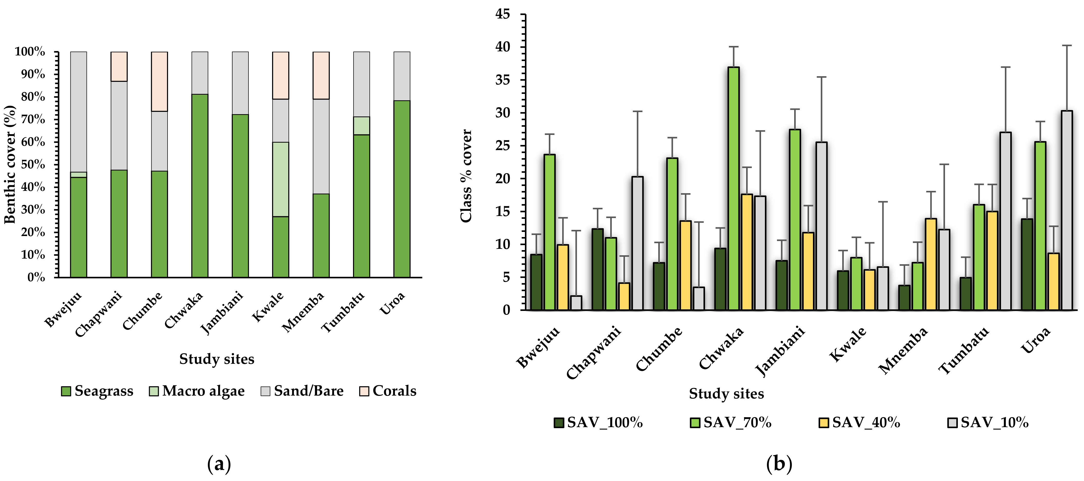
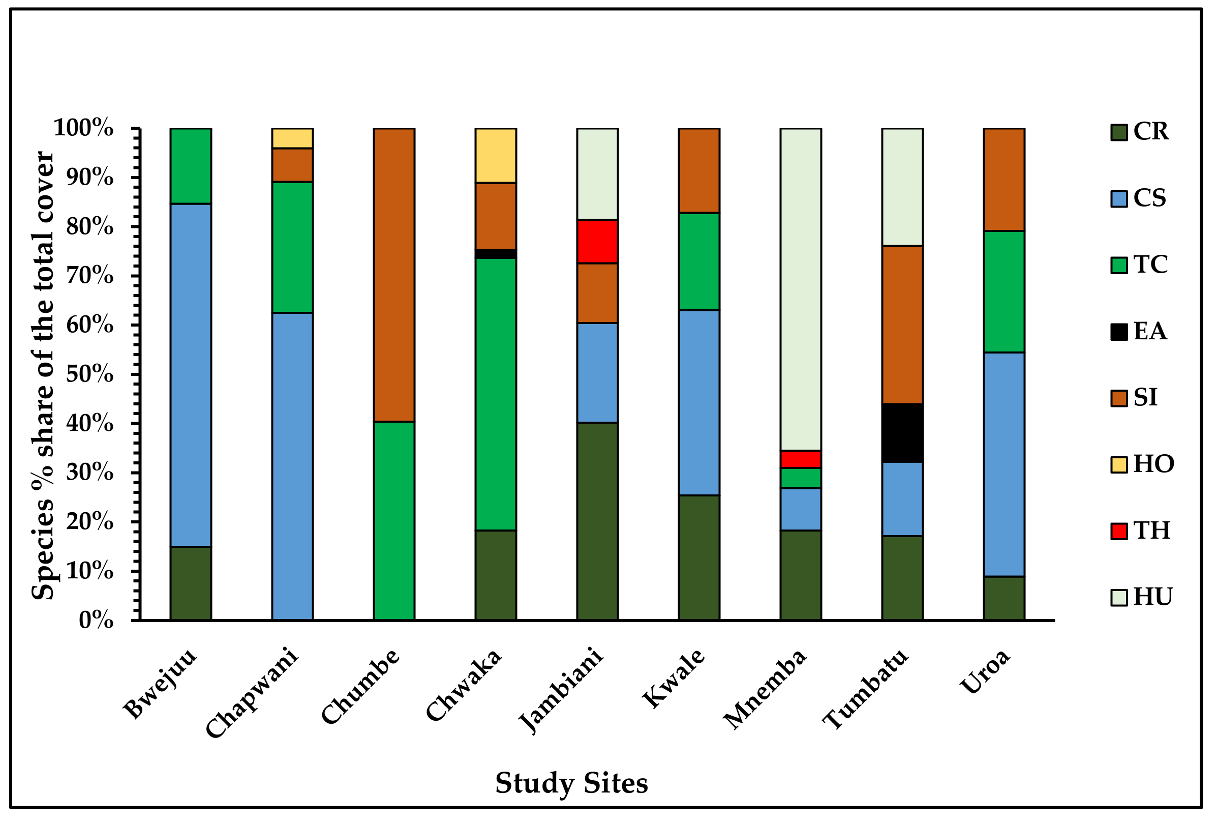
Benthic Classes, Percent Cover, and Cover of Seagrass Species

The seagrasses accounted for 55% of the total area (492.6 ha), 31% of the bare sediment, 9% of the coral substrates, and only 5% for the macroalgae. The highest proportion (33%) of macroalgae in all the mapped seascapes was in Kwale (Figure 6a). This site also had a larger area with a hard/rock substratum, compared to all the other sites dominated by Ulva (Figure 6a). Other sites with shares of macroalgae at significant contributions were Tumbatu (8%) and Bwejuu (2.4%) (Figure 6a). Whereas coral reefs frequently co-occurred with seagrass in nearly all the areas, this habitat type had a higher percent contribution from Chumbe (25%), Kwale (21%), Mnemba (21%), and Chapwani (13%) (Figure 6a). At the Bwejuu site, we recorded the highest percentage of the bare substrate (53%) of the total area mapped (Figure 6a).

The seagrass total percent cover was assessed for four classes, representing continuous cover (70–100%), dense cover (40–70%), moderate cover (10–40%), and low cover (1–10%). On average, for all nine sites, the dense cover class was the highest (19.8%), followed by the low cover class at 16.1% (Figure 6b). The moderate and continuous classes had 11% and 8.1%, respectively (Figure 6b). Among the nine sites, Mnemba and Tumbatu had the lowest cover for the 70–100% class, with 3.7% and 4.9%, respectively. In contrast, high seagrass densities in Uroa (13.8%) and Chapwani (12.3%) were observed for the 70–100% class. The low-density class dominated in Uroa (30.3%), Tumbatu (27.0%), and Jambiani (25.5%) (Figure 6b).

Of the nine seagrass species identified, eight species were distinguished by drone images (Figure 7). Four of these species, namely, TC (45%), CS (30%), CR (29%), and SI (28%), were abundant in all nine sites. By contrast, Thalassia hemprichii, Enhalus acoroides, Halodule uninervis, and Halophila ovalis were only shown in the cover maps of Jambiani, Uroa, Tumbatu, Chwaka, Mnemba, and Chapwani, with varied cover proportions (Figure 7 and Figure S3). Only Halophila stipulacea was observed from underwater photos in very small patches, so that it was not possible to show its cover in any of the maps (Figure S2).

3.3. Seagrass Distribution with Depth

Both the benthic classes and the seagrass total covers varied with the depth gradient in the Zanzibar waters, with the total seagrass share decreasing from 30.1 to 1.6% between 1-m and 5-m depths (Figure 8a). Likewise, the species occurrence (species diversity) and the species percent cover for each of the depth intervals show a falling trend, from eight species in 1 to 2 m, to three species at 5-m depth intervals. The proportion of species in 1 m contributed more by 63% for TC, 53% for CS, and 47% for SI. The species EA, SI, HU, and TC were also recorded at the depth of 5 m (Figure 8b). The species, HU, was the most prevalent in each depth interval, followed by SI (Figure 8b). The species, CS and CR, were more abundant within 1 to 3 m (Figure 8b). Site-wise, the Kwale site had more cover spread (65%), to the depths of 2–3 m, 2–4 m, and 4–5 m, than any other site. The Chwaka and Tumbatu sites, on the other hand, had higher cover within 1 to 2 m, while the Jambiani site had higher cover within 2–4 m (Table S4).

3.4. Patchiness of the Seagrass Seascapes

To assess the levels of the patchiness of the seagrass meadows, we applied three categories, highly patchy, moderate patchy, and less patchy, for our description. The meadows that fell under the “highly patchy” category were those that recorded high numbers of patches (NP) and patch densities (PD = number/100 hectares), compared with the other sites. The results show that Jambiani, with maximum NP and DP values of 38,235 and 39,233, was under this category (Figure 9a). Sites such as Chumbe, with values of 3650 for NP and 20,112 for DP, and Bwejuu, with values of 9890 for NP and 16,828 for DP, were classified under the “moderate patchy” category. On the other hand, the meadows of Chwaka, which had the lowest values (NP:838; PD: 978), Mnemba (NP: 3427; PD: 3428), and Uroa (NP: 1436; PD: 4431) were designated as “less patchy” meadows (Figure 9a).

Considering the patch size metric (AREA_MN), only Jambiani remained the most patchy meadow, with an average patch size of 0.00273 ha (about 27.3 m²), of all the seagrass meadows mapped (Figure 9b). By contrast, the Chapwani site had a large mean patch area, with a value of 3.67 ha (33,700 m²). The standard deviation of the mean patch size for all nine sites was 1.15 ha (about 11,500 m²). The other descriptors of the meadows’ patchiness characterizing the configuration and cohesiveness of the seascapes (Table S5) include the LPI, which was highest in Chapwani (43.6%), and the GYRATE_MN, which showed a slight variation among the sites, from 0.92 m in Chwaka, to 0.361 m for Kwale (Table S5), and the SD = 0.173 m (Table S5). The LD index measured further fragmentation and it showed that Jambiani had a maximum value = 1.0; Chwaka recorded a minimum value = 0.375, and the SD was 0.211 in all nine sites (Table S5). Overall, three sites recorded high LD indexes, from 0.9–1, four sites had LD indexes ranging from 0.8–0.6, and one site had an index value of 0.5–0.4 (Table S5).

The results also show that Jambiani, a site characterized by high patchiness (Figure 9, Table S5), also had a quarter of its cover (25.5%) under the low-cover class (Figure 6). By contrast, the Chwaka site, a least patchy area, with a mean patch size of approx 18 m² (Figure 9b), had more than one-third (36.9%) of its cover under the dense-cover class (Figure 6). We also examined if the differences across the seagrass species exist with patchiness with the largest patch index (LPI) and the total core area (TCA). The results show that the sites with higher shares of the species, Thalassodenron ciliatum, Enhalus acoroides, and Cymodocea serrulata, also had high LPI index values and were characterized with low patchiness (Table S5). These meadows were Chwaka, Tumbatu, and Uroa (Table S5). The correlation for LPI with the T. ciliatum species was 0.71, and the correlation for TCA with T.ciliatum was 0.60.

3.5. Associated Flora and Fauna in Seagrass Meadows

3.5.1. Epiphytes and Dead Leaves

Chwaka and Uroa had the highest epiphytic loadings (26.3 and 24.9%, respectively) while the dead leaves were accounted for more by the Uroa (30%) and Chapwani (22%) sites (Figure 10a). The sites along the main coast (Uroa, Chwaka, Tumbatu, Chapwani, and, to lesser extent, Jambiani) had higher epiphyte loadings (26%), compared to the more remote islet sites (15%) (Figure 10b). Species-wise, TC, EA, and CS were more overgrown by epiphytes (Figure S4). The highest percentages of dead leaves were observed in Uroa, Mnemba, and Jambiani, and were, furthermore, affected by desiccation (Figure S3 for visualization).

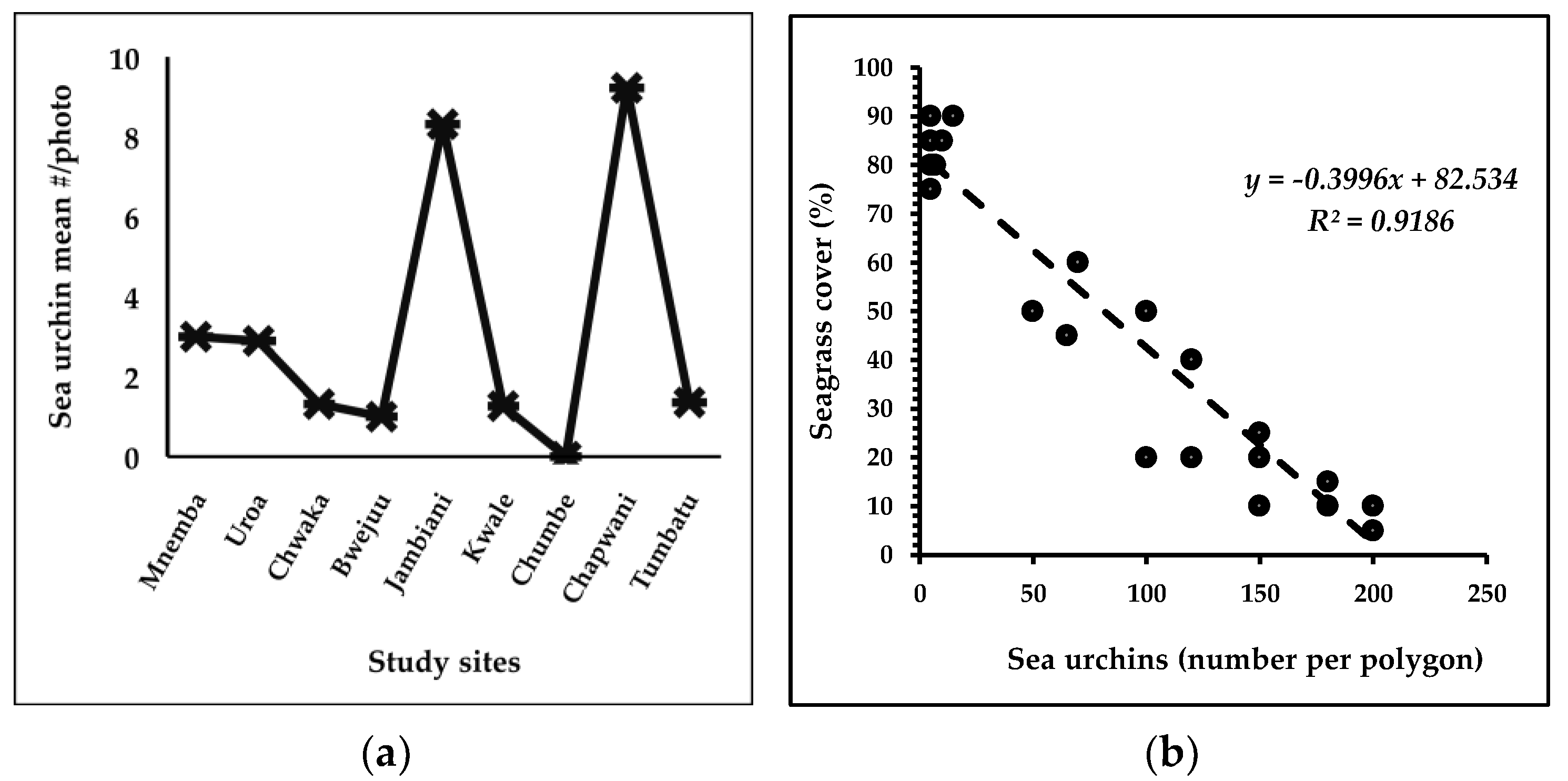
3.5.2. Sea Urchin Interaction with Seagrass Habitats

An analysis of the in situ photos showed a threefold higher density of sea urchins at Chapwani and Jambiani, with total counts of 710 and 290, respectively (Figure 11a). An analysis of the sea urchin density association with the seagrass cover in Chapwani, based on the feature detection method, showed that the seagrass cover correlated negatively (r² = 0.9, p < 0.01) with the sea urchin density (Figure 11b).

The results also reveal that the moderate-cover class (10–40%) had the highest share of sea urchins (71%) and the continuous-cover class (70–100%) had the lowest sea urchin share (2.2%) (Figure S5a). Furthermore, the low-cover areas of the Cymodocea serrulata (Chapwani) and Thalassia hemprichii (Jambiani) meadows had high densities of sea urchins (Figure S5b,c)

3.6. Multivariate Analysis

We applied ANOSIM to test the hypothesis stating that there is no difference across the sites. The result for the sample statistic, Global R, was 0.488, with an overall p-value of 0.1%, indicating that the nine sites were significantly different. A pairwise comparison showed that all, except four site comparisons, were significantly different (p = 0.8%), and that the sites could be clustered into three groups (1: Jambiani; 2: Chumbe, Bwejuu, Mnemba, and Kwale; and 3: Chapwani, Uroa, Tumbatu, and Chwaka). Significant differences were also found when comparing the five depth groups (Global R of 0.074, with an overall p-value of 1.3%), indicating that, regardless of the sites, there were significant changes in the biotic features with increasing depth. The differences between the sites and with depth were visualized on a 2D metric MDS ordination plot, with a stress value of 0.22, indicating a robust ordination of the data (Figure 12).

Interestingly, the pairwise analysis of the differences indicated higher variations between pairs that were far apart by depths, i.e., 1–3 m, 1–4 m, and 1–5 m, than the neighboring ones, i.e., 1–2 m, 2–3 m and 4–5 m, indicating an overall gradual transition in the biotic features with depth. In support of this, the mMDS plot shows a relatively higher variation within Depths 1 and 2, than for Depths 4 and 5 (Figure 12), revealing high variations of the observed community of seagrass metrics at shallow depths, rather than at deeper depths.

4. Discussion

This study investigated the application of aerial drone imagery, in combination with in situ photos, to map tropical-seagrass-dominated coastal areas, and it provides the information needed to characterize the ecosystem health of these important nearshore subtidal habitats. The drone-based information included: (a) Depth-specific quantitative data on the cover of seagrasses, macroalgae, corals, and the substrate habitat aerial extent; (b) Data on the diversity of the habitat typology and the seagrass species; and (c) Data on the patchiness of the seagrasses. With these data layers, we characterized nine sites with information relevant for a habitat health assessment [44,45,46,48]. Furthermore, integrating the drone imagery with spatial reference points, and visually assessing in situ photos, aided the imagery classification and the extraction of crucial information on other elements for the characterization of the seagrass habitat conditions, such as the sea urchins in the seagrass cover [90], and assessment of the epiphytic cover and dead leaves [47].

4.1. Spatial Characterization of Tropical Nearshore Habitats Using Drone Imagery

4.1.1. Cover Maps

Aerial drone imagery is increasingly being applied in order to generate spatially referenced assessments of the health conditions in shallow-water marine habitats [40,50,54,58,91]. The three types of maps produced, benthic cover maps, seagrass total cover maps, and seagrass species cover maps, describe the seascape habitats of the subtidal water commonly examined in many studies [32,33,52,56]. Previous efforts to map the Zanzibar seagrass habitats were based on more coarse satellite imagery [31,32]. In contrast, we applied a locally adaptable approach to the data acquisition. While this approach has been applied in the temperate region [40,50,54,58], to the best of our knowledge, it marks a new development in the WIO region.

Benthic Classes, Seagrass Total Cover, and Species Composition

The high drone delineation accuracy of the habitat types—seagrasses, corals, macroalgae, and bare—in the nine-nearshore sites, revealed the very diverse habitats of these areas. Whereas previous studies point to the general complex pattern [2,27,31], a more detailed estimate was possible with drone imagery under this study. Particularly, seagrasses were significant habitats in the nine investigated sites, contributing to more than half (55%) of the total area (724 ha) mapped. Interestingly, the coral reefs of the mapped sites mostly occurred around the small islet sites, compared to sites closer to the main coast, highlighting the importance of these islet areas for coral reef conservation. The occurrence of macroalgae was typically higher in areas with extensive rocky substrates, such as in Kwale and Tumbatu. By contrast, seagrasses were more prevalent in areas dominated by sandy substrates. Such a complex pattern has been revealed previously [31,92], and it implies that the habitat composition follows the suitable substrate conditions, which concurs with a previous study [32], and with studies beyond Zanzibar [2,93,94].

Overall, the sites had seagrass densities mostly in the 40–70% category, while they had the fewest in the 70–100% class, indicating that the seagrass cover was not generally continuous, but consisted of rather fragmented patches of moderate cover. The intraclass coefficients of variation in all nine sites were highest in the 1–10% class, and lowest in the 70–100% class, suggesting that the variability, i.e., the patchiness, decreased as the meadows became denser [49].

The species composition is critical in the health characterization of the seagrass meadows [44,45,95], and is a pertinent output of remote sensing classifications [33,52,96]. Combining aerial drones with in situ observations, we documented a high seagrass species richness across the mapped sites, with nine species in total, dominated by Thalassodendron ciliatum, Cymodocea serrulata, Cymodocea rotundata, and Syringodium isoetifolium. Furthermore, the interspecies interaction was clearly marked with the co-occurrence of, on average, three species, typically entangled together in many sites. Our drone-based observations confirmed the high seagrass species diversity of the Zanzibar waters, as revealed in previous studies, where species numbers between six and eight have been reported [1,2,31]. Two seagrass species—Nanozostera capensis and Halodule wrighthii—identified by [32], were not observed in our study, indicating that they are very rare species, and/or, for the case of Halodule wrighthii, that there is confusion in the species identification, as has been reported by [84].

Interestingly, the seagrass cover differed for the species. For instance, Thalassodendron ciliatum in Chapwani and Cymodcea serrulata in Uroa had more continuous cover than the Syringodium isoetifolium species, which was very sparsely distributed. Likewise, all of the sites where Thalassodendron ciliatum and Enhalus acoroides were observed appeared as dense and continuous meadows, owing to their big leaves and higher growth, contrary to the Halophila ovalis, which was associated with a sparse arrangement, likely because of their size and because they are a pioneer species [84]. In other studies, the dynamics in the spatial patterning of seagrasses have been linked with the species nature [95]. Our results underscore the high potential of the drone-based mapping of seagrass-species-specific cover.

From the onset, mapping complex meadows, as presented in this work, is faced with the constraints of delineating distinct co-occurring species in the dynamic shallow-water environments. It is widely known that remote sensing outputs for species cover are likely to suffer from very similar spectral signatures of these species [50,53,71]. However, compared with the Landsat-8- and Sentinel-2-based classifications implemented previously [31,32], drone imagery enabled us to perform a more detailed analysis of the gradients in the seagrass density, and to distinguish between the dominant species, as it has been demonstrated by [59], which is essential information for explaining the governing conditions for seagrass distribution.

4.1.2. Accuracy Assessment

Assessing the accuracy of the cover maps is essential for determining the performance of the remote-sensing-based classifications [52,82,97]. We followed a conventional approach to this assessment [33,52,56]. Our classification approach resulted in high accuracy values that were within acceptable ranges (94% to the lowest, 71%) for remote-sensing-based classification outputs. In general, the results imply higher performances for the benthic cover classes (seagrass, corals, macroalgae, bare), and lower performances for the maps of the seagrass species, indicating that the spectral signatures of the seagrass species can be difficult to distinguish [33,37,52]. Coral reefs were sometimes confused with bare substrate, even though the bare substrate had higher delineation values. A part of this uncertainty seems to arise from the differences in the coral species, but it is also related to the complexity arising from the mix of live and dead corals and rocks in some sites, for example, in the Chapwani site.

Other factors that may have contributed to the limitations of the RGB imagery performed are the environmental conditions during mapping, which include the sun angle, waves, and clouds, as pointed out by [40,50]. While we reduced the effects of these factors on the acquired imagery by avoiding days with high winds and cloud cover, and collected imagery around noon to lessen the impact of sun glint, future applications should be enhanced with a more rigorous algorithm [98]. Furthermore, we optimized the data quality by ensuring a high overlap (80%) between scenes, mapping at a low altitude to obtain a high resolution (average 2.4 cm), and by using GPS points during the image processing in Agisoft Metashape to enhance the agreement of the orthomosaics with the real environment. The imagery precision could be further enhanced with the permanent markers with poles [66] and, if available, the use of RTK/PPK drones. Generally, compared with previous applications, our approach provides high accuracy and high-resolution maps of the benthic cover, total seagrass cover, and species cover [37,40,50,54,58], which is attributable to good weather conditions, clear waters, and distinguishable optical signatures.

4.2. Depth Distribution of Seagrasses

The seagrass cover with bathymetry suggested that, in shallow depths, the physical disturbances were more pronounced, and, at greater depths, the light defined the cover [69,99]. This was shown by the clear decrease in the seagrass cover with depth, within the depth interval of 1 to 5 m. Similarly, we found a decline in the species richness and the cover of specific species as the depth increased. While there are no separate studies that have examined the seagrass depth distribution in Zanzibar, declining cover with depth is a well-expected pattern [99]. Interestingly, higher variability in the cover within a 1–2 m depth, compared to deeper (4–5 m) zones, was revealed, indicating a more variable shallow environment that is influenced by physical exposure, heat stress, and the tidal range [100], but that is also likely more strongly impacted by the human-based activities on the seagrass meadows [7,20,101,102]. The shallow depth variations in the seagrass cover could be explained by human impacts. In Jambiani, for instance, the seagrass meadows were highly interrupted with seaweed farms within the 1–2 m zone, compared to the deeper 3- to 4-m depths, which explains why the more continuous cover was observed at 3-to-4-m depths. In comparison, the seagrass meadows were denser in the shallow intertidal areas of Tumbatu and Chwaka, where there were no seaweed farms. In contrast, Kwale, a site characterized by a steeper bathymetry, had higher seagrass cover at higher depths (4–5 m), indicating that other factors, such as the substrate conditions and the wave exposure, may play critical roles in determining the local depth distributions [24,101].

We observed quite large variations in the depth distributions of the dominant seagrass species, with notable differences between the nine sites. As an example, Thallasodendron ciliatum dominated at shallow depths in Chwaka, compared to Kwale, where it dominated at greater depths (3–5 m), indicating differences in the growth conditions and an ability to adapt to these [1,2,27], in addition to the interspecies competition. Enhalus acoroides, on other hand, often occurred in the deep pools and streams in the Chwaka and Tumbatu sites (Table S2), supporting previous evidence in the WIO region [1,2,84,100]. Implied in the species distribution explained here is that favorable growth conditions vary between species, enabling them to coexist and occupy different niches [1,100]. Further understanding of the optimal growth conditions for different seagrass species, in combination with remotely sensed spatial observations, will help explain the differences in the distributions of the seagrass species with depth, and provide valuable information on the importance of the environmental conditions underlying the seagrass habitat distribution [37].

4.3. Patchiness of Seagrass Distributions

We applied statistical principles from landscape ecology to determine the patterns in the distributions of the seagrass coverage, which are likely a response to different human pressures on the seascapes [39,73,103,104], with an emphasis on investigating the structures and functionalities of marine habitats, as in [24,49,73,105]. Using drone images, our study was the first to characterize the patchiness of the seagrass habitats in the waters around Zanzibar. Patchiness was here defined as a static feature of seascape fragmentation [24,39], and was applied to understand the nature and levels of the pressures on the seascape structure [24,39,72].

The mapped areas could be grouped as “highly patchy” meadows (Jambiani, Bwejuu, Chumbe), “moderately patchy” meadows” (Kwale, Chapwani, Tumbatu), and “less patchy” meadows (Uroa, Mnemba, Chwaka). The selected patchiness indices (Table S1) can help us to quantitatively assess the levels of pressure that these meadows have been, or are currently, undergoing [24,73]. For instance, the fragmentation indices at the patch levels, such as the NP and PD, and at the landscape level, such as the LD, were higher in the sites classified as “highly patchy”. The patch number in this group was higher, while the size of these patches was considerably small, relative to the other seascapes mapped. Not surprisingly, sites under the “less patchy” category were those with large patch sizes, a high percent in PLAND, and low values on the LD. That is to say, the less patchy meadows were generally associated with a more continuous cover and connectedness than the meadows under the “highly patchy” category.

Thanks to the drone imagery high resolution, the patchiness indices captured the fine seascape structure changes within the meadows, which are important for determining the levels of physical and human pressures, the meadow functionality, and the overall seagrass health, as it has been applied by [24,49,72,73,106]. However, being a first-time analysis of the seagrass fragmentation in the Zanzibar meadows, there is no immediate reference to compare with, or to determine if changes have occurred. Yet, because of the many disturbances affecting the seagrasses in the WIO and Zanzibar, in particular [20,27,28], climate change [18,107], and the increasing interest in blue carbon trapping [108,109], the mapping and seascape structure analysis of the seagrass habitats can be readily applied in order to gauge the functionality and integrity of seagrass meadows and prioritize conservation measures [110].

4.4. Characterization of Habitats Using In Situ Imagery

The results on the epiphytic loadings implied three generic groups of these sites—"high epiphytic” loadings (above 20% cover), such as in Uroa and Chwaka, “moderate epiphytic” loadings for Chapwani, and Tumbatu, and “low epiphytic” loadings, with values of not more than 6%, for Chumbe, Jambiani, Bwejuu, Mnemba, and Kwale. The high epiphytic loadings on the seagrass leaves seem partly related to the configuration of the intertidal areas and the species differences. Relatively close subtidal waters (Chwaka and Tumbatu sites) had higher loadings compared to more open systems with more efficient water exchanges (Kwale and Chumbe sites). Similarly, certain species—Thallasodendron ciliatum and Enhalus acoroides—were linked with moderate-to-high epiphytic loadings, compared to Syringondium isoetifolium. This explanation agrees with the authors of [111], who suggest that the nature of the intertidal areas and the water movements influence the overall epiphytic development, and who found higher epiphytic loadings on Thallasodendron ciliatum and Enhalus acoroides meadows.

Sea urchins play an important herbivory role, affecting the density of seagrass meadows [90,112,113]. We observed large differences in the densities of sea urchins among the nine sites, with the largest densities in Chapwani and Jambiani. This occurrence was high in low-seagrass-cover spots, implying the potential effect of sea urchins on the seagrass cover [90,113,114,115]. Interestingly, the sea urchin signature was strong enough to be detected by the drone imagery, demonstrating the method’s high ability for retrieving information beyond the traditional seagrass cover in clear shallow-water conditions [24,40,50].

4.5. Multivariate Classification of Nearshore Seagrass Habitats

We tested the null hypothesis of no significant differences across sites by using an analysis of variance (ANOSIM), and we highlighted the major groups in the mMDS ordination plot using all the collected biotic and abiotic data. The multivariate analysis indicates that there was significant intersite variability associated with the differences in the fragmentation and distribution of the percent cover, along with the depth profile. Furthermore, the nine sites could be statistically categorized into three main groups, with Jambiani as the most unique, compared to the other two groups. This uniqueness could be explained by its higher fragmentation values and by the high variation at depths of 1 to 2 m. The ANOSIM statistically based classification of the nine sites aligned well with the narrative description from the in situ data (Table S2), which describes the variations in the percent cover, seagrass-depth distribution, and fragmentation as most prominent in the very shallow bathymetry, compared to further offshore. The three identified groups of sites were further different in terms of the site remoteness, the percent cover with depth, the level of fragmentation, the sea urchin density, and the epiphytic loadings. Such information about the site differences could be a useful base for future research from which to investigate the underlying environmental conditions governing the differences in nearshore seagrass-dominated areas. Thus, the classification could be used for the future ecological health assessment of the status of seagrass, for instance, through the development of seagrass habitat health indices, which are important tools for marine ecosystem management [44,46]. Further applications could be enhanced with more replicate data on the biotic features, which were not available during this analysis.

5. Conclusions

In this study, we demonstrated the utility of drone imagery for mapping and characterizing the habitat conditions of tropical shallow-water marine environments, an important step in monitoring marine ecosystems, such as those dominated by seagrasses [2,50,58]. While such an approach has been applied in other parts of the world [37,40,50,54,58], this was a novel mapping method for nearshore marine habitats in the tropical waters of Zanzibar (WIO region), where seagrasses are currently in decline because of multiple pressures [2,3,4,20,27,28,116,117,118]. Improved datasets on the distributions and compositions of seagrasses provide important gateways to the effective management of these essential habitats [1,2]. We show that this approach has great applicability in the mapping of seagrass-dominated habitats, and that it can be utilized to provide detailed information on a range of important parameters of seagrass habitats, such as the habitat typology, the horizontal and depth distributions, the diversity, and the seascape fragmentation.

Methodologically, we show that drone imagery, when integrated with in situ data, provide very information-rich datasets, of which many cannot be established with commonly used in situ methods alone. While the satellite-based method is regarded as optimal for continuous large-scale marine monitoring [37,38,55,71], it is of limited use for local-scale habitat observations [38]. More often, generating a detailed classification for shallow-water marine habitats with satellite-generated data is hampered by the varied dynamics in this zone and the weather [37,38]. Even though aerial photography from crewed aircraft is in wide use and could provide monthly photos [119], it is expensive and may not be as easily adapted to the local conditions. By comparison, the method demonstrated here provided highly accurate results that are suitable for detailed shallow-water marine habitat mapping at the local scale, as has also been shown in temperate systems [38,40,50,91]. Given the limited institutional capacity and limited marine ecosystem management systems, which are hindered by technological and financial constraints [28,120], it is paramount to adopt a rapid cost-effective method, as was demonstrated here, in this region of the WIO. Moving forward, future studies on seagrass-dominated habitats are recommended to further examine the association of the identified habitat health parameters with important environmental parameters, such as temperature, salinity, exposure, and human influence.

References

1. Bandeira, S.; Björk, M. Seagrass research in the eastern Africa region: Emphasis on diversity, ecology and ecophysiology. S. Afr. J. Bot. 2001, 67, 420–425. [Google Scholar] [CrossRef] [Green Version]
2. Gullström, M.; de la Torre Castro, M.; Bandeira, S.O.; Björk, M.; Dahlberg, M.; Kautsky, N.; Rönnbäck, P.; Öhman, M.C. Seagrass Ecosystems in the Western Indian Ocean. AMBIO J. Hum. Environ. 2002, 31, 588–596. [Google Scholar] [CrossRef]
3. Cullen-Unsworth, L.C.; Nordlund, L.M.; Paddock, J.; Baker, S.; McKenzie, L.J.; Unsworth, R.K. Seagrass meadows globally as a coupled social-ecological system: Implications for human wellbeing. Mar. Pollut. Bull. 2014, 83, 387–397. [Google Scholar] [CrossRef] [PubMed]
4. De la Torre-Castro, M.; Di Carlo, G.; Jiddawi, N.S. Seagrass importance for a small-scale fishery in the tropics: The need for seascape management. Mar. Pollut. Bull. 2014, 83, 398–407. [Google Scholar] [CrossRef]
5. Lugendo, B.R.; Nagelkerken, I.; van der Velde, G.; Mgaya, Y.D. The importance of mangroves, mud and sand flats, and seagrass beds as feeding areas for juvenile fishes in Chwaka Bay, Zanzibar: Gut content and stable isotope analyses. J. Fish Biol. 2006, 69, 1639–1661. [Google Scholar] [CrossRef]
6. Lyimo, T.J.; Mvungi, E.F.; Lugomela, C.; Björk, M. Seagrass Biomass and Productivity in Seaweed and Non-Seaweed Farming Areas in the East Coast of Zanzibar, Tanzania. West. Indian Ocean J. Mar. Sci. 2006, 5, 141–152. [Google Scholar]
7. De la Torre-Castro, M.; Rönnbäck, P. Links between humans and seagrasses—an example from tropical East Africa. Ocean Coast. Manag. 2004, 47, 361–387. [Google Scholar] [CrossRef]
8. Msuya, F.E.; Namukose, M.; Beltran-Gutierrez, M.; Fabiani, G.; Kunzmann, A. Integrated seaweed–sea cucumber farming in Tanzania. West. Indian Ocean J. Mar. Sci. 2018, 17, 35–50. [Google Scholar]
9. Greiner, J.T.; McGlathery, K.J.; Gunnell, J.; McKee, B.A. Seagrass restoration enhances “blue carbon” sequestration in coastal waters. PLoS ONE 2013, 8, e72469. [Google Scholar] [CrossRef] [Green Version]
10. Röhr, M.E.; Boström, C.; Canal-Vergés, P.; Holmer, M. Blue carbon stocks in Baltic Sea eelgrass (Zostera marina) meadows. Biogeosciences 2016, 13, 6139–6153. [Google Scholar] [CrossRef] [Green Version]
11. Bulthuis, D.A.; Brand, G.W.; Mobley, M.C. Suspended sediments and nutrients in water ebbing from seagrass-covered and denuded tidal mudflats in a southern Australian embayment. Aquat. Bot. 1984, 20, 257–266. [Google Scholar] [CrossRef]
12. Fonseca, M.S. Sediment stabilization by Halophila decipiens in comparison to other seagrasses. Estuarine Coast. Shelf Sci. 1989, 29, 501–507. [Google Scholar] [CrossRef]
13. Koch, E.W. Hydrodynamics of a shallow Thalassia testudinum bed in Florida, USA. In Seagrass Biology, Proceedings of an International Workshop, Rottnest Island, Australia, 25–29 January 1996; University of Western Australia: Perth, Australia, 1996; pp. 25–29. [Google Scholar]
14. James, R.K.; Christianen, M.J.A.; van Katwijk, M.M.; de Smit, J.C.; Bakker, E.S.; Herman, P.M.J.; Bouma, T.J. Seagrass coastal protection services reduced by invasive species expansion and megaherbivore grazing. J. Ecol. 2020, 108, 2025–2037. [Google Scholar] [CrossRef]
15. Orth, R.J.; Carruthers, T.J.; Dennison, W.C.; Duarte, C.M.; Fourqurean, J.W.; Heck, K.L.; Hughes, A.R.; Kendrick, G.A.; Kenworthy, W.J.; Olyarnik, S. A global crisis for seagrass ecosystems. Bioscience 2006, 56, 987–996. [Google Scholar] [CrossRef] [Green Version]
16. Waycott, M.; Duarte, C.M.; Carruthers, T.J.; Orth, R.J.; Dennison, W.C.; Olyarnik, S.; Calladine, A.; Fourqurean, J.W.; Heck, K.L.; Hughes, A.R. Accelerating loss of seagrasses across the globe threatens coastal ecosystems. Proc. Natl. Acad. Sci. USA 2009, 106, 12377–12381. [Google Scholar] [CrossRef] [Green Version]
17. Short, F.T.; Polidoro, B.; Livingstone, S.R.; Carpenter, K.E.; Bandeira, S.; Bujang, J.S.; Calumpong, H.P.; Carruthers, T.J.B.; Coles, R.G.; Dennison, W.C.; et al. Extinction risk assessment of the world’s seagrass species. Biol. Conserv. 2011, 144, 1961–1971. [Google Scholar] [CrossRef]
18. Amone-Mabuto, M.; Bandeira, S.; da Silva, A. Long-term changes in seagrass coverage and potential links to climate-related factors: The case of Inhambane Bay, southern Mozambique. West. Indian Ocean J. Mar. Sci. 2017, 16, 13–25. [Google Scholar]
19. Short, F.T.; Wyllie-Echeverria, S. Natural and human-induced disturbance of seagrasses. Environ. Conserv. 1996, 23, 17–27. [Google Scholar] [CrossRef]
20. Khamis, Z.A.; Kalliola, R.; Käyhkö, N. Spatial modelling of cumulative human pressure in the tropical coastscape of Zanzibar, Tanzania. Afr. J. Mar. Sci. 2019, 41, 337–352. [Google Scholar] [CrossRef]
21. Ralph, P.J.; Tomasko, D.; Moore, K.; Seddon, S.; Macinnis, O.C.M. Human impacts on seagrasses: Eutrophication, sedimentation, and contamination. In Seagrasses: Biology, Ecology, and Conservation; Springer: Dordrecht, The Netherlands, 2007; pp. 567–593. [Google Scholar]
22. Yaakub, S.M.; McKenzie, L.J.; Erftemeijer, P.L.A.; Bouma, T.; Todd, P.A. Courage under fire: Seagrass persistence adjacent to a highly urbanised city–state. Mar. Pollut. Bull. 2014, 83, 417–424. [Google Scholar] [CrossRef]
23. Hallac, D.E.; Sadle, J.; Pearlstine, L.; Herling, F.; Shinde, D. Boating impacts to seagrass in Florida Bay, Everglades National Park, Florida, USA: Links with physical and visitor-use factors and implications for management. Mar. Freshw. Res. 2012, 63, 1117–1128. [Google Scholar] [CrossRef] [Green Version]
24. Abadie, A.; Gobert, S.; Bonacorsi, M.; Lejeune, P.; Pergent, G.; Pergent-Martini, C. Marine space ecology and seagrasses. Does patch type matter in Posidonia oceanica seascapes? Ecol. Indic. 2015, 57, 435–446. [Google Scholar] [CrossRef]
25. Serrano, O.; Ruhon, R.; Lavery, P.S.; Kendrick, G.A.; Hickey, S.; Masqué, P.; Arias-Ortiz, A.; Steven, A.; Duarte, C.M. Impact of mooring activities on carbon stocks in seagrass meadows. Sci. Rep. 2016, 6, 23193. [Google Scholar] [CrossRef]
26. Lyimo, T.J.; Mvungi, E.F.; Mgaya, Y.D. Abundance and diversity of seagrass and macrofauna in the intertidal areas with and without seaweed farming activities in the east coast of Zanzibar. Tanzan. J. Sci. 2008, 34, 41–52. [Google Scholar] [CrossRef] [Green Version]
27. Stæhr, P.A.; Sheikh, M.; Rashid, R.; Ussi, A.; Suleiman, M.; Kloiber, U.; Dahl, K.; Tairova, Z.; Strand, J.; Kuguru, B. Managing human pressures to restore ecosystem health of zanzibar coastal waters. J. Aquac. Mar. Biol. 2018, 7, 59–70. [Google Scholar] [CrossRef] [Green Version]
28. Khamis, Z.A.; Kalliola, R.; Käyhkö, N. Geographical characterization of the Zanzibar coastal zone and its management perspectives. Ocean Coast. Manag. 2017, 149, 116–134. [Google Scholar] [CrossRef]
29. Lange, G.-M. Tourism in Zanzibar: Incentives for sustainable management of the coastal environment. Ecosyst. Serv. 2015, 11, 5–11. [Google Scholar] [CrossRef]
30. Shah, N.J.; Lindén, O.; Lundin, C.G.; Johnstone, R. Coastal management in Eastern Africa: Status and future. Ambio 1997, 26, 227–234. [Google Scholar]
31. Gullström, M.; Lundén, B.; Bodin, M.; Kangwe, J.; Öhman, M.C.; Mtolera, M.S.P.; Björk, M. Assessment of changes in the seagrass-dominated submerged vegetation of tropical Chwaka Bay (Zanzibar) using satellite remote sensing. Estuarine Coast. Shelf Sci. 2006, 67, 399–408. [Google Scholar] [CrossRef]
32. Knudby, A.; Nordlund, L. Remote sensing of seagrasses in a patchy multi-species environment. Int. J. Remote Sens. 2011, 32, 2227–2244. [Google Scholar] [CrossRef]
33. Phinn, S.; Roelfsema, C.; Dekker, A.; Brando, V.; Anstee, J. Mapping seagrass species, cover and biomass in shallow waters: An assessment of satellite multi-spectral and airborne hyper-spectral imaging systems in Moreton Bay (Australia). Remote Sens. Environ. 2008, 112, 3413–3425. [Google Scholar] [CrossRef]
34. Nordlund, L.M.; Unsworth, R.K.F.; Gullström, M.; Cullen-Unsworth, L.C. Global significance of seagrass fishery activity. Fish Fish. 2018, 19, 399–412. [Google Scholar] [CrossRef]
35. Hedberg, N.; von Schreeb, K.; Charisiadou, S.; Jiddawi, N.S.; Tedengren, M.; Nordlund, L.M. Habitat preference for seaweed farming—A case study from Zanzibar, Tanzania. Ocean Coast. Manag. 2018, 154, 186–195. [Google Scholar] [CrossRef]
36. Poursanidis, D.; Traganos, D.; Teixeira, L.; Shapiro, A.; Muaves, L. Cloud-native seascape mapping of Mozambique’s Quirimbas National Park with Sentinel-2. Remote Sens. Ecol. Conserv. 2021, 7, 275–291. [Google Scholar] [CrossRef]
37. Kutser, T.; Hedley, J.; Giardino, C.; Roelfsema, C.; Brando, V.E. Remote sensing of shallow waters—A 50 year retrospective and future directions. Remote Sens. Environ. 2020, 240, 111619. [Google Scholar] [CrossRef]
38. Lønborg, C.; Thomasberger, A.; Stæhr, P.A.U.; Stockmarr, A.; Sengupta, S.; Rasmussen, M.L.; Nielsen, L.T.; Hansen, L.B.; Timmermann, K. Submerged aquatic vegetation: Overview of monitoring techniques used for the identification and determination of spatial distribution in European coastal waters. Integr. Environ. Assess. Manag. 2021, n/a. [Google Scholar] [CrossRef]
39. Boström, C.; Pittman, S.J.; Simenstad, C.; Kneib, R.T. Seascape ecology of coastal biogenic habitats: Advances, gaps, and challenges. Mar. Ecol. Prog. Ser. 2011, 427, 191–217. [Google Scholar] [CrossRef] [Green Version]
40. Nahirnick, N.K.; Reshitnyk, L.; Campbell, M.; Hessing-Lewis, M.; Costa, M.; Yakimishyn, J.; Lee, L.; Horning, N.; Poursanidis, D. Mapping with confidence; delineating seagrass habitats using Unoccupied Aerial Systems (UAS). Remote Sens. Ecol. Conserv. 2018, 5, 121–135. [Google Scholar] [CrossRef]
41. Galparsoro, I.; Pınarbaşı, K.; Gissi, E.; Culhane, F.; Gacutan, J.; Kotta, J.; Cabana, D.; Wanke, S.; Aps, R.; Bazzucchi, D.; et al. Operationalisation of ecosystem services in support of ecosystem-based marine spatial planning: Insights into needs and recommendations. Mar. Policy 2021, 131, 104609. [Google Scholar] [CrossRef]
42. Yang, W.; Zhang, Z.; Sun, T.; Liu, H.; Shao, D. Marine ecological and environmental health assessment using the pressure-state-response framework at different spatial scales, China. Ecol. Indic. 2021, 121, 106965. [Google Scholar] [CrossRef]
43. Roca, G.; Alcoverro, T.; Krause-Jensen, D.; Balsby, T.J.S.; van Katwijk, M.M.; Marbà, N.; Santos, R.; Arthur, R.; Mascaró, O.; Fernández-Torquemada, Y.; et al. Response of seagrass indicators to shifts in environmental stressors: A global review and management synthesis. Ecol. Indic. 2016, 63, 310–323. [Google Scholar] [CrossRef] [Green Version]
44. Neto, J.M.; Barroso, D.V.; Barría, P. Seagrass Quality Index (SQI), a Water Framework Directive compliant tool for the assessment of transitional and coastal intertidal areas. Ecol. Indic. 2013, 30, 130–137. [Google Scholar] [CrossRef]
45. Marbà, N.; Krause-Jensen, D.; Alcoverro, T.; Birk, S.; Pedersen, A.; Neto, J.M.; Orfanidis, S.; Garmendia, J.M.; Muxika, I.; Borja, A. Diversity of European seagrass indicators: Patterns within and across regions. Hydrobiologia 2013, 704, 265–278. [Google Scholar] [CrossRef]
46. Purvaja, R.; Robin, R.; Ganguly, D.; Hariharan, G.; Singh, G.; Raghuraman, R.; Ramesh, R. Seagrass meadows as proxy for assessment of ecosystem health. Ocean Coast. Manag. 2018, 159, 34–45. [Google Scholar] [CrossRef]
47. Nelson, W.G. Development of an epiphyte indicator of nutrient enrichment: Threshold values for seagrass epiphyte load. Ecol. Indic. 2017, 74, 343–356. [Google Scholar] [CrossRef]
48. Halpern, B.S.; Longo, C.; Hardy, D.; McLeod, K.L.; Samhouri, J.F.; Katona, S.K.; Kleisner, K.; Lester, S.E.; O’Leary, J.; Ranelletti, M.; et al. An index to assess the health and benefits of the global ocean. Nature 2012, 488, 615–620. [Google Scholar] [CrossRef] [Green Version]
49. Sleeman, J.C.; Kendrick, G.A.; Boggs, G.S.; Hegge, B.J. Measuring fragmentation of seagrass landscapes: Which indices are most appropriate for detecting change? Mar. Freshw. Res. 2005, 56, 851–864. [Google Scholar] [CrossRef]
50. Duffy, J.P.; Pratt, L.; Anderson, K.; Land, P.E.; Shutler, J.D. Spatial assessment of intertidal seagrass meadows using optical imaging systems and a lightweight drone. Estuarine Coast. Shelf Sci. 2018, 200, 169–180. [Google Scholar] [CrossRef]
51. Lathrop, R.G., Jr.; Haag, S.M.; Merchant, D.; Kennish, M.J.; Fertig, B. Comparison of remotely-sensed surveys vs. in situ plot-based assessments of sea grass condition in Barnegat Bay-Little Egg Harbor, New Jersey USA. J. Coast. Conserv. 2004, 2014, 299–308. [Google Scholar] [CrossRef]
52. Roelfsema, C.M.; Lyons, M.; Kovacs, E.M.; Maxwell, P.; Saunders, M.I.; Samper-Villarreal, J.; Phinn, S.R. Multi-temporal mapping of seagrass cover, species and biomass: A semi-automated object based image analysis approach. Remote Sens. Environ. 2014, 150, 172–187. [Google Scholar] [CrossRef]
53. Stæhr, P.A.; Groom, G.B.; Krause-Jensen, D.; Hansen, L.B.; Huber, S.; Jensen, L.Ø.; Rasmussen, M.B.; Upadhyay, S.; Ørberg, S.B. Use of Remote Sensing Technologies for Monitoring Chlorophyll A and Submerged Aquatic Vegetation in Danish Coastal Waters: Part of the Restek Project; Aarhus University, DCE—Danish Centre for Environment and Energy: Roskilde, Denmark, 2019. [Google Scholar]
54. Ventura, D.; Bruno, M.; Jona Lasinio, G.; Belluscio, A.; Ardizzone, G. A low-cost drone based application for identifying and mapping of coastal fish nursery grounds. Estuarine Coast. Shelf Sci. 2016, 171, 85–98. [Google Scholar] [CrossRef]
55. Harvey, T.; Krause-Jensen, D.; Stæhr, P.A.; Groom, G.B.; Hansen, L.B. Literature Review of Remote Sensing Technologies for Coastal Chlorophyll-A Observations and Vegetation Coverage; Technical Report from DCE—Danish Centre for Environment and Energy No. 112; Aarhus University, DCE—Danish Centre for Environment and Energy: Roskilde, Denmark, 2018; 47p, Available online: http://dce2.au.dk/pub/TR112.pdf (accessed on 15 December 2021).
56. Roelfsema, C.M.; Phinn, S.R.; Udy, N.; Maxwell, P. An integrated field and remote sensing approach for mapping Seagrass Cover, Moreton Bay, Australia. J. Spat. Sci. 2009, 54, 45–62. [Google Scholar] [CrossRef]
57. Andriolo, U.; Gonçalves, G.; Rangel-Buitrago, N.; Paterni, M.; Bessa, F.; Gonçalves, L.M.S.; Sobral, P.; Bini, M.; Duarte, D.; Fontán-Bouzas, Á.; et al. Drones for litter mapping: An inter-operator concordance test in marking beached items on aerial images. Mar. Pollut. Bull. 2021, 169, 112542. [Google Scholar] [CrossRef]
58. Konar, B.; Iken, K. The use of unmanned aerial vehicle imagery in intertidal monitoring. Deep Sea Res. Part II Top. Stud. Oceanogr. 2018, 147, 79–86. [Google Scholar] [CrossRef]
59. Monteiro, J.G.; Jiménez, J.L.; Gizzi, F.; Přikryl, P.; Lefcheck, J.S.; Santos, R.S.; Canning-Clode, J. Novel approach to enhance coastal habitat and biotope mapping with drone aerial imagery analysis. Sci. Rep. 2021, 11, 574. [Google Scholar] [CrossRef] [PubMed]
60. Knudby, A.; LeDrew, E.; Brenning, A. Predictive mapping of reef fish species richness, diversity and biomass in Zanzibar using IKONOS imagery and machine-learning techniques. Remote Sens. Environ. 2010, 114, 1230–1241. [Google Scholar] [CrossRef]
61. Knudby, A.; Nordlund, L.M.; Palmqvist, G.; Wikström, K.; Koliji, A.; Lindborg, R.; Gullström, M. Using multiple Landsat scenes in an ensemble classifier reduces classification error in a stable nearshore environment. Int. J. Appl. Earth Obs. Geoinf. 2014, 28, 90–101. [Google Scholar] [CrossRef]
62. Maina, J.; Venus, V.; McClanahan, T.R.; Ateweberhan, M. Modelling susceptibility of coral reefs to environmental stress using remote sensing data and GIS models. Ecol. Model. 2008, 212, 180–199. [Google Scholar] [CrossRef]
63. Blakey, T.; Melesse, A.; Hall, M. Supervised Classification of Benthic Reflectance in Shallow Subtropical Waters Using a Generalized Pixel-Based Classifier across a Time Series. Remote Sens. 2015, 7, 5098–5116. [Google Scholar] [CrossRef] [Green Version]
64. Duro, D.C.; Franklin, S.E.; Dubé, M.G. A comparison of pixel-based and object-based image analysis with selected machine learning algorithms for the classification of agricultural landscapes using SPOT-5 HRG imagery. Remote Sens. Environ. 2012, 118, 259–272. [Google Scholar] [CrossRef]
65. Blaschke, T. Object based image analysis for remote sensing. ISPRS J. Photogramm. Remote Sens. 2010, 65, 2–16. [Google Scholar] [CrossRef] [Green Version]
66. Fallati, L.; Saponari, L.; Savini, A.; Marchese, F.; Corselli, C.; Galli, P. Multi-Temporal UAV Data and Object-Based Image Analysis (OBIA) for Estimation of Substrate Changes in a Post-Bleaching Scenario on a Maldivian Reef. Remote Sens. 2020, 12, 2093. [Google Scholar]
67. Zhang, C. Applying data fusion techniques for benthic habitat mapping and monitoring in a coral reef ecosystem. ISPRS J. Photogramm. Remote Sens. 2015, 104, 213–223. [Google Scholar] [CrossRef]
68. Román, A.; Tovar-Sánchez, A.; Olivé, I.; Navarro, G. Using a UAV-Mounted Multispectral Camera for the Monitoring of Marine Macrophytes. Front. Mar. Sci. 2021, 8, 1225. [Google Scholar] [CrossRef]
69. Duarte, C.M.; Kirkman, H. Methods for the measurement of seagrass abundance and depth distribution. In Global Seagrass Research Methods, 1st ed.; Short, F., Coles, R., Eds.; Elsevier: Amsterdam, The Netherlands, 2001. [Google Scholar]
70. Fauzan, M.A.; Kumara, I.S.W.; Yogyantoro, R.N.; Suwardana, S.W.; Fadhilah, N.; Nurmalasari, I.; Apriyani, S.; Wicaksono, P. Assessing the Capability of Sentinel-2A Data for Mapping Seagrass Percent Cover in Jerowaru, East Lombok. Indones. J. Geogr. 2017, 49, 195–203. [Google Scholar] [CrossRef] [Green Version]
71. Ferwerda, J.G.; de Leeuw, J.; Atzberger, C.; Vekerdy, Z. Satellite-based monitoring of tropical seagrass vegetation: Current techniques and future developments. Hydrobiologia 2007, 591, 59–71. [Google Scholar] [CrossRef]
72. Flowers, B.; Huang, K.-T.; Aldana, G.O. Analysis of the Habitat Fragmentation of Ecosystems in Belize Using Landscape Metrics. Sustainability 2020, 12, 3024. [Google Scholar] [CrossRef] [Green Version]
73. Wedding, L.M.; Lepczyk, C.A.; Pittman, S.J.; Friedlander, A.M.; Jorgensen, S. Quantifying seascape structure: Extending terrestrial spatial pattern metrics to the marine realm. Mar. Ecol. Prog. Ser. 2011, 427, 219–232. [Google Scholar] [CrossRef] [Green Version]
74. DHI GRAS. Satellite-Derived Bathymetry: Mapping and Measuring Water Depths from Space. Available online: https://www.dhi-gras.com/solutions/satellite-derived-bathymetry/ (accessed on 15 December 2021).
75. Guzinski, R.; Spondylis, E.; Michalis, M.; Tusa, S.; Brancato, G.; Minno, L.; Hansen, L.B. Exploring the Utility of Bathymetry Maps Derived With Multispectral Satellite Observations in the Field of Underwater Archaeology. Open Archaeol. 2016, 2. [Google Scholar] [CrossRef] [Green Version]
76. Klonowski, W.; Fearns, P.; Lynch, M. Retrieving key benthic cover types and bathymetry from hyperspectral imagery. J. Appl. Remote Sens. 2007, 1, 011505. [Google Scholar] [CrossRef]
77. Lee, Z.; Carder, K.L.; Chen, R.F.; Peacock, T.G. Properties of the water column and bottom derived from Airborne Visible Infrared Imaging Spectrometer (AVIRIS) data. J. Geophys. Res. Ocean. 2001, 106, 11639–11651. [Google Scholar] [CrossRef] [Green Version]
78. Lee, Z.; Carder, K.L.; Mobley, C.D.; Steward, R.G.; Patch, J.S. Hyperspectral remote sensing for shallow waters: 2. Deriving bottom depths and water properties by optimization. Appl. Opt. 1999, 38, 3831–3843. [Google Scholar] [CrossRef] [Green Version]
79. Lee, Z.; Carder, K.L.; Mobley, C.D.; Steward, R.G.; Patch, J.S. Hyperspectral remote sensing for shallow waters. I. A semianalytical model. Appl. Opt. 1998, 37, 6329–6338. [Google Scholar] [CrossRef]
80. Fethers, J.O. Remote Sensing of Eelgrass using Object Based Image Analysis and Sentinel-2 Imagery. Master’s Thesis, University of Aalborg, Aalborg, Denmark, 2018; p. 95. [Google Scholar]
81. Lillesand, T.; Kiefer, R.W.; Chipman, J. Remote Sensing and Image Interpretation; John Wiley & Sons: New Jersey, NJ, USA, 2015; p. 736. [Google Scholar]
82. McKenzie, L.; Campbell, S.; Roder, C. Seagrass-Watch: Manual for Mapping & Monitoring Seagrass Resources by Community (Citizen) Volunteers; Information Series Qi01094; Northern Fisheries Centre: Townsville, Australia, 2003. [Google Scholar]
83. McKenzie, L.J.; Finkbeiner, M.A.; Kirkman, H. Methods for mapping seagrass distribution. In Global Seagrass Research Methods, 1st ed.; Short, F., Coles, R., Eds.; Elsevier: Amsterdam, The Netherlands, 2001; pp. 101–121. [Google Scholar]
84. Richmond, M.D. (Ed.) A Field Guide to the Seashores of Eastern Africa and the Western Indian Ocean Islands, 3rd ed.; Sida/WIOMSA: Dar es Salaam, Tanzania, 2011; p. 464. [Google Scholar]
85. Hesselbarth, M.H.K.; Sciaini, M.; With, K.A.; Wiegand, K.; Nowosad, J. landscapemetrics: An open-source R tool to calculate landscape metrics. Ecography 2019, 42, 1648–1657. [Google Scholar] [CrossRef] [Green Version]
86. Miller-Myers, R.; Virnstein, R.W. Development and Use of an Epiphyte Photo-Index (EPI) for Assessing Epiphyte Loadings on the Seagrass Halodule wrightii; CRC Press: Boca Raton, FL, USA, 2000. [Google Scholar]
87. Schreeb, K.V. Mapping Coastal Biotopes and Resource Use in Zanzibar, Tanzania. Master’s Thesis, Stockholm University, Stockholm, Sweden, 2016. [Google Scholar]
88. Bray, J.R.; Curtis, J.T. An ordination of the upland forest communities of southern Wisconsin. Ecol. Monogr. 1957, 27, 326–349. [Google Scholar] [CrossRef]
89. Clarke, K.; Gorley, R. PRIMER v7: User Manual/Tutorial; Primer-E Ltd.: Plymouth, UK, 2015. [Google Scholar]
90. Eklöf, J.S.; de la Torre-Castro, M.; Gullström, M.; Uku, J.; Muthiga, N.; Lyimo, T.; Bandeira, S.O. Sea urchin overgrazing of seagrasses: A review of current knowledge on causes, consequences, and management. Estuarine Coast. Shelf Sci. 2008, 79, 569–580. [Google Scholar] [CrossRef]
91. Aoki, L.R.; McGlathery, K.J.; Wiberg, P.L.; Oreska, M.P.J.; Berger, A.C.; Berg, P.; Orth, R.J. Seagrass Recovery Following Marine Heat Wave Influences Sediment Carbon Stocks. Front. Mar. Sci. 2021, 7, 1170. [Google Scholar] [CrossRef]
92. Gullström, M.; Lyimo, T.J.; Eklöf, J.S.; Björk, M.; Semesi, I.S.; de la Torre-Castro, M. Seagrass meadows in Chwaka Bay: Socio-ecological and management aspects. In People, Nature and Research in Chwaka Bay, Zanzibar, Tanzania; De la Torre-Castro, M., Lyimo, T.J., Eds.; Western Indian Ocean Marine Science Association (WIOMSA): Zanzibar, Tanzania, 2012; p. 346. [Google Scholar]
93. Dan, A.; Moriguchi, A.; Mitsuhashi, K.; Terawaki, T. Relationship between Zostera marina beds and bottom sediments, and wave action offshore in Naruto, southern Japan. Fish. Eng. 1998, 34, 299–304. [Google Scholar]
94. Stæhr, P.A.; Göke, C.; Holbach, A.M.; Krause-Jensen, D.; Timmermann, K.; Upadhyay, S.; Ørberg, S.B. Habitat Model of Eelgrass in Danish Coastal Waters: Development, Validation and Management Perspectives. Front. Mar. Sci. 2019, 6, 175. [Google Scholar] [CrossRef] [Green Version]
95. Kendrick, G.A.; Holmes, K.W.; Van Niel, K.P. Multi-Scale Spatial Patterns of Three Seagrass Species with Different Growth Dynamics. Ecography 2008, 31, 191–200. [Google Scholar] [CrossRef]
96. Koedsin, W.; Intararuang, W.; Ritchie, R.J.; Huete, A. An Integrated Field and Remote Sensing Method for Mapping Seagrass Species, Cover, and Biomass in Southern Thailand. Remote Sens. 2016, 8, 292. [Google Scholar] [CrossRef] [Green Version]
97. Hossain, M.S.; Bujang, J.S.; Zakaria, M.H.; Hashim, M. The application of remote sensing to seagrass ecosystems: An overview and future research prospects. Int. J. Remote Sens. 2014, 36, 61–114. [Google Scholar] [CrossRef]
98. Giles, A.B.; Davies, J.E.; Ren, K.; Kelaher, B. A deep learning algorithm to detect and classify sun glint from high-resolution aerial imagery over shallow marine environments. ISPRS J. Photogramm. Remote Sens. 2021, 181, 20–26. [Google Scholar] [CrossRef]
99. Duarte, C.M. Seagrass depth limits. Aquat. Bot. 1991, 40, 363–377. [Google Scholar] [CrossRef]
100. Aleem, A.A. Distribution and ecology of seagrass communities in the Western Indian Ocean. Deep Sea Res. Part A Oceanogr. Res. Pap. 1984, 31, 919–933. [Google Scholar] [CrossRef]
101. Fonseca, M.S.; Bell, S.S. Influence of physical setting on seagrass landscapes near Beaufort, North Carolina, USA. Mar. Ecol. Prog. Ser. 1998, 171, 109–121. [Google Scholar] [CrossRef] [Green Version]
102. Wikström, K. Influence of Landscape Configuration and Within-Patch Variation on Fish Abundance, Size and Functional Groups in Tropical Seagrass Beds; Stockholm University: Stockholm, Sweden, 2013. [Google Scholar]
103. Hinchey, E.K.; Nicholson, M.C.; Zajac, R.N.; Irlandi, E.A. Preface: Marine and coastal applications in landscape ecology. Landsc. Ecol. 2008, 23, 1–5. [Google Scholar] [CrossRef]
104. Li, X.; Mander, Ü. Future options in landscape ecology: Development and research. Prog. Phys. Geogr. Earth Environ. 2009, 33, 31–48. [Google Scholar] [CrossRef]
105. Ortiz Cajica, A.K.; Hinojosa-Arango, G.; Garza-Pérez, J.R.; Rioja-Nieto, R. Seascape metrics, spatio-temporal change, and intensity of use for the spatial conservation prioritization of a Caribbean marine protected area. Ocean Coast. Manag. 2020, 194, 105265. [Google Scholar] [CrossRef]
106. Vermaat, J.E.; Rollon, R.N.; Lacap, C.D.A.; Billot, C.; Alberto, F.; Nacorda, H.M.E.; Wiegman, F.; Terrados, J. Meadow fragmentation and reproductive output of the SE Asian seagrass Enhalus acoroides. J. Sea Res. 2004, 52, 321–328. [Google Scholar] [CrossRef]
107. Björk, M.; Short, F.; McLeod, E.; Beer, S. Managing Seagrasses for Resilience to Climate Change; IUCN International Union for Conservation of Nature: Gland, Switzerland, 2008; Volume 3. [Google Scholar]
108. Gullström, M.; Lyimo, L.D.; Dahl, M.; Samuelsson, G.S.; Eggertsen, M.; Anderberg, E.; Rasmusson, L.M.; Linderholm, H.W.; Knudby, A.; Bandeira, S.; et al. Blue Carbon Storage in Tropical Seagrass Meadows Relates to Carbonate Stock Dynamics, Plant–Sediment Processes, and Landscape Context: Insights from the Western Indian Ocean. Ecosystems 2018, 21, 551–566. [Google Scholar] [CrossRef] [Green Version]
109. Macreadie, P.I.; Anton, A.; Raven, J.A.; Beaumont, N.; Connolly, R.M.; Friess, D.A.; Kelleway, J.J.; Kennedy, H.; Kuwae, T.; Lavery, P.S.; et al. The future of Blue Carbon science. Nat. Commun. 2019, 10, 3998. [Google Scholar] [CrossRef] [Green Version]
110. Cuevas, E.; Uribe-Martínez, A.; Morales-Ojeda, S.M.; Gómez-Ruíz, P.A.; Núñez-Lara, E.; Teutli-Hernández, C.; Herrera-Silveira, J.A. Spatial configuration of seagrass community attributes in a stressed coastal lagoon, southeastern Gulf of Mexico. Reg. Stud. Mar. Sci. 2021, 48, 102049. [Google Scholar] [CrossRef]
111. Leliaert, F.; Vanreusel, W.; De Clerck, O.; Coppejans, E. Epiphytes on the seagrasses of Zanzibar Island (Tanzania), floristic and ecological aspects. Belg. J. Bot. 2001, 134, 3–20. [Google Scholar]
112. Mamboya, F.; Lugomela, C.; Mvungi, E.; Hamisi, M.; Kamukuru, A.T.; Lyimo, T.J. Seagrass–sea urchin interaction in shallow littoral zones of Dar es Salaam, Tanzania. Aquat. Conserv. Mar. Freshw. Ecosyst. 2009, 19, S19–S26. [Google Scholar] [CrossRef]
113. Valentine, J.F.; Heck, K.L. The role of sea urchin grazing in regulating subtropical seagrass meadows: Evidence from field manipulations in the northern Gulf of Mexico. J. Exp. Mar. Biol. Ecol. 1991, 154, 215–230. [Google Scholar] [CrossRef]
114. Carnell, P.E.; Ierodiaconou, D.; Atwood, T.B.; Macreadie, P.I. Overgrazing of Seagrass by Sea Urchins Diminishes Blue Carbon Stocks. Ecosystems 2020, 23, 1437–1448. [Google Scholar] [CrossRef]
115. Rose, C.D.; Sharp, W.C.; Kenworthy, W.J.; Hunt, J.H.; Lyons, W.G.; Prager, E.J.; Valentine, J.F.; Hall, M.O.; Whitfield, P.E.; Fourqurean, J.W. Overgrazing of a large seagrass bed by the sea urchin Lytechinus variegatus in Outer Florida Bay. Mar. Ecol. Prog. Ser. 1999, 190, 211–222. [Google Scholar] [CrossRef]
116. Eklöf, J.S.; Henriksson, R.; Kautsky, N. Effects of tropical open-water seaweed farming on seagrass ecosystem structure and function. Mar. Ecol. Prog. Ser. 2006, 325, 73–84. [Google Scholar] [CrossRef]
117. Zanzibar Planning Commission. Human Pressure and Threats on Coastal and Marine Resources, Zanzibar: A Critical Review; Zanzibar Planning Commission: Zanzibar, Tanzania, 2017; p. 135.
118. Nchimbi, A.A.; Lyimo, L.D. Socioeconomic Determinants of Mangrove Exploitation and Seagrass Degradation in Zanzibar: Implications for Sustainable Development. J. Mar. Biol. 2019, 2019, 7684924. [Google Scholar] [CrossRef] [Green Version]
119. Meehan, A.J.; Williams, R.J.; Watford, F.A. Detecting Trends in Seagrass Abundance Using Aerial Photograph Interpretation: Problems Arising with the Evolution of Mapping Methods. Estuaries 2005, 28, 462–472. [Google Scholar] [CrossRef]
120. Unsworth, R.K.F.; van Keulen, M.; Coles, R.G. Seagrass meadows in a globally changing environment. Mar. Pollut. Bull. 2014, 83, 383–386. [Google Scholar] [CrossRef] [PubMed]
Figure 1. Delineation of nine sites for drone mapping around Unguja Island, Zanzibar. The nine sites are marked with red and bolded names. Blue colors represent depth contours derived from a Sentinel 2 images from June 2018 [74]. Green areas are mangroves, based on the Zanzibar Department of Forestry data.
Remotesensing 14 00680 g001
Figure 2. Steps involved in the planning, execution, and processing of drone images for seagrass mapping. We developed our approach following recommendations by [50]. Steps 111 correspond to the decisions made for: (12) the site selection, where S2 imagery, literature, and reconnaissance surveys were used; drone planning in (3) flight design, including choice of optimal days for mapping; (4) drone image capturing; (5) in situ data collection to create waypoints with GPS receiver, and photo quadrats and videos with Paralenz camera and underwater drones. In step (6), data organization involved post-field data preparation for processing, this included checking for data accuracy, data entry, and creating vector spatial layers; (7) data processing, where we transformed individual photos into orthomosaics with Agisoft and transferred the tiff files into the ArcGIS environment for the creation of an integrated geodatabase ready for step (8), in which the OBIA classification was performed. In step (9), validation and accuracy, the assessment was executed with reimplementation of maximum likelihood algorithm (MLA) if the classification was not to the desirable accuracy, and, if desirable, step (10) followed to allow for the production of classified cover maps, and these cover maps were used to undertake, in step (11), the fragmentation analysis with the landscapemetrics R package.
Remotesensing 14 00680 g002
Figure 3. Example of field data integration for habitat characterization: (a,b) are field data for the Uroa site, presenting (a) seagrass percent cover, and (b) seagrass species composition; (c,d) are drone imagery scenes from the Chapwani site presenting a feature-detection method for sea urchins; (c) a drone mosaic, and (d) the portion of one of the sea urchins’ hotspots in the site that could be detected (Section 2.3.5. for full description).
Remotesensing 14 00680 g003
Figure 4. An example of classified cover map output: (a) benthic cover (BC) presenting four major classes (if all) present (bare; corals; seagrasses; and macroalgae); (b) seagrass total cover map (TC), including bare area. The classes are: bare; 1–10% (low cover); 10–40% (moderate cover); 40–70% (dense cover); and 70–100% (continuous cover); (c) thematic map of the seagrass species cover presented with only dominant species—here, four species (Cymodocea serrulata, Cymodocea rotundata, Syringodium isoetifolium, and Thalassodendron ciliatum); (df) are the statistics corresponding to each of the cover maps, (ac), respectively. A more detailed spatial distribution of the mapped classes is clearly shown in a 6-m scale with (i), (ii), and (iii).
Remotesensing 14 00680 g004
Figure 5. Performances of different classification types with user accuracy in yellow, and producer accuracy in green: (a) benthic classes; (b) total seagrass classes; and (c) species classification. In (c), species are: Thalassodendron ciliatum (TC); Thalassia Hemprichii (TH); Cymodcea serrulata (CS); Cymodocea rotundata (CR); Halodule uninervis (HU); Syringodium isoetifolium (SI); and Enhalus acoroides (EA). Macroalgae (MA) were also included during the classification type. The species, Halophila ovalis, only had significant cover in one site (Chapwani) and had 78% and 70% user and producer accuracy performances, respectively. The in-depth confusion matrix is presented in Table S3A–C of the Supplementary Materials.
Remotesensing 14 00680 g005
Figure 6. Comparison of (a) the benthic classes, and (b) seagrass total cover from nine nearshore sites around Unguja Island.
Remotesensing 14 00680 g006
Figure 7. Dominant species cover distribution across sites: Cymodocea rotundata (CR); Cymodcea serrulate (CS); Thalassodendron ciliatum (TC); Enhalus acoroides (EA); Syringodium isoetifolium (SI); Halophila ovalis (HO); Thalassia hemprichii (TH); and Halodule uninervis (HU).
Remotesensing 14 00680 g007
Figure 8. Seagrass distribution with depth: (a) total seagrass cover, and (b) species cover. Species: Cymodocea serrulata (CS); Cymodocea rotundata (CR); Thalassodendron ciliatum (TC); Halophila ovalis (HO); Enhalus acoroides (EA); Halodule uninervis (HU); Syringodium isoetifolium (SI); and Thalassia hemprichii (TH).
Remotesensing 14 00680 g008
Figure 9. Descriptors of seagrass patchiness: (a) the number of patches (NP) has no unit as it is a count of the observed number of seagrass patches; the patch density (PD) is a measure of the density of the seagrass patches, expressed as the number per 100 hectares; (b) patch size is presented as a mean area of the patches in the seagrass class and is expressed in hectares.
Remotesensing 14 00680 g009
Figure 10. Epiphytic loadings and dead leaves estimates, according to (a) nine sites, and (b) the coastal type.
Remotesensing 14 00680 g010
Figure 11. Sea urchin abundance in seagrass meadows: (a) frequency of sea urchins (two species dominated: Diadema setosum and Echinometra mathaei), identified from photo points at the nine study sites; (b) from analysis drone images, the sea urchin densities (number per drone mapped polygon, n = 27) were compared with the total cover of seagrass in the Chapwani area.
Remotesensing 14 00680 g011
Figure 12. The mMDS ordination plot visualizes the similarities among the nine sites. Each site is separated into five depth intervals. Full lines outline groups with similar biotic and abiotic features identified from the ANOSIM analysis. The numbers 1–5 represents depth replicates.
Remotesensing 14 00680 g012