Abstract
For a variational data assimilation (DA) system that assimilates radiance observations, the simulated brightness temperature (BT) at the top of the atmosphere and the corresponding Jacobians carried out by the radiance observation operator are needed information. Previous studies reported that the incorporation of aerosol information into the radiance observation operator leads to cooler simulated infrared (IR) BTs and warmer temperature analyses at low levels of the atmosphere. However, the role of the aerosol-affected Jacobians in the DA system, which not only affect the determination of analysis increments but also influence the quality control and the bias correction algorithm, is yet to be investigated. This study examines the aerosol impacts on the sensitivity of IR radiance simulations, Jacobians, and the analysis increments by conducting two experiments: (i) sensitivity tests to assess how the different aspects of the aerosol profiles (i.e., mass loading, peak aerosol level, aerosol thickness layer, and bin partition) affect the simulated BT and the Jacobians from the Community Radiative Transfer Model (CRTM), which is the radiance observation operator in the Gridpoint Statistical Interpolation (GSI) analysis system; (ii) single IR observation experiments using GSI to investigate how the aerosol-affected atmospheric Jacobians influence the analysis increment. The results show that dust aerosols produce the strongest cooling to simulated BTs under similar aerosol optical depths; simulated BTs and Jacobians are most sensitive to the loading and peak altitude of the aerosol layer; simulated BTs become more sensitive to the temperature of the aerosol layer; aerosol-induced differences in atmospheric Jacobians lead to considerable changes to temperature and moisture increments. These results provide a better understanding of the aerosol impacts on each component involved in radiance DA, which can provide guidance for assimilating aerosol-affected IR observations.
1. Introduction
Satellite radiance observations in the units of equivalent brightness temperature (BT) at the top of the atmosphere have been directly assimilated at many operational numerical weather prediction (NWP) centers since the early 1990s [1,2,3,4]. To directly assimilate satellite radiance observations, a fast and accurate radiative transfer model (RTM) is required as the forward operator. The RTMs used in data assimilation (DA) systems simulate the BTs based on the atmospheric states from the NWP model (e.g., temperature, water vapor mixing ratio, etc.). They also apply tangent-linear and adjoint methods to calculate the linearized operator (i.e., Jacobians), which is the first derivative of BTs with respect to model states, for the conversion between model and observation space. In variational DA systems, the analysis increment is determined by the first-guess BT departures (observed BTs minus simulated BTs) weighted with the background errors, observation errors, and the Jacobians [5]. The two most widely used RTMs for DA are the Radiative Transfer model for the Television Infrared Observation Satellite (TIROS) Operational Vertical Sounder (TOVS) (RTTOV) [6] and the Community Radiative Transfer Model (CRTM) [7,8].
Previous studies have demonstrated that simulated BTs can be decidedly colder in the thermal infrared (IR) window region when RTMs consider aerosol transmittance (absorption/scattering) effects. For example, Sokolik [9] and Pierangelo et al. [10] revealed that the heavy loading of mineral dust aerosols could generate up to 10 K of BT cooling in the IR window region. Using RTTOV, Matricardi [11] and Quan et al. [12] compared the BT cooling effects between different aerosol types (e.g., urban, desert, etc.) defined in the Optical Properties of Aerosols and Clouds package (OPAC) [13]. Both reported that the desert aerosol produces the strongest cooling effects in the IR window region. Using CRTM, Liu et al. [14] demonstrated BT cooling in CRTM by incorporating a profile with organic carbon and dust aerosols for the IR window channels of the High-resolution Infrared Radiation Sounder (HIRS). Chen et al. [15] also observed small aerosol cooling effects on the simulated BTs by CRTM when comparing the simulated BTs with and without aerosol information for oceanic observations at the three IR channels of the Advanced Very High Resolution Radiometer (AVHRR).
Previous studies have further demonstrated that low-level analyzed temperatures are warmer when considering the aerosol transmittance effects on IR radiance simulations [16,17,18]. In Weaver et al. [16], the temperature retrievals considering dust contamination were assimilated. Instead of temperature retrievals, Kim et al. [17] and Wei et al. [18] incorporated the aerosol information into the BT simulation of the radiance observation operator to assess the aerosol impacts on meteorological analyses. To do this, both studies conducted two Gridpoint Statistical Interpolation (GSI) experiments, which utilized CRTM handling the BT simulations. For the two experiments, one cycled experiment excluded aerosol transmittance effects (the baseline); the other included aerosol transmittance effects in BT simulations, but the experiment used the first guesses from the baseline (i.e., the aerosol-aware offline). By assimilating identical sets of observations and first guesses in both GSI experiments, the differences between the experiments clearly demonstrate the response of meteorological analyses to the aerosol-aware BT simulations carried out by CRTM. It should be noted that quality control (QC) [19] and bias correction (BC) [20] algorithms in GSI were not modified; these are designed to assimilate clear-sky IR observations only.
In GSI, the aerosol-induced changes in the CRTM simulations of IR observations would affect the analyses through three components. Their synthetical impacts on analyses have been reported but not investigated thoroughly in Kim et al. [17] and Wei et al. [18]. These include:
- cooler simulated BTs, which produce larger positive first-guess departures that then cause the warming features on the temperature analyses. The bias-corrected first-guess departures are utilized in QC.
- aerosol-affected Jacobians for surface temperature and surface emissivity, which are utilized by QC and BC algorithms, respectively. Moreover, the Jacobian for surface temperature is involved in the determination of sea surface temperature analysis.
- changes to the Jacobians for atmospheric states, which are not only involved in the minimization of the cost function to determine the analysis increments but also the cloud check in QC.
However, several unanswered questions arise. For example, although many prior studies have demonstrated aerosol impacts on simulated BTs, what is the sensitivity of the BT simulations to the characteristics of aerosol profiles that represent various scenarios? For the surface Jacobians, what are the aerosol-induced changes and how do they influence the QC check of “skin temperature sensitivity” and biases estimated by the surface emissivity predictor, respectively? For example, Wei et al. [18] showed that more IR window observations passed QC over land and the positive biases estimated by BC were reduced. For the atmospheric Jacobians, how strong, and at what atmospheric levels, are the changes induced by aerosol information and thus how do those changes influence the analysis increments?
Motivated by the questions above, this study systematically investigates each aspect of the aerosol impacts on the IR radiance observations in the DA system. To do this, we will conduct two experiments: (i) CRTM sensitivity tests with prescribed aerosol profiles under a fixed atmospheric state. This experiment will better understand how different aerosol profiles influence the simulated BTs and Jacobians. These results will also provide insights about the uncertainties for assimilating aerosol-affected IR observations, such as the systematic biases. (ii) GSI single IR observation test with and without aerosol information. Given identical model states and first-guess departures, this experiment will isolate the impacts of aerosol-affected atmospheric Jacobians on the vertical distribution of analysis increments. Moreover, these results will provide insight into the complexity of how the atmospheric Jacobians affect the analysis fields (e.g., how the water vapor and temperature Jacobians together affect the temperature analysis).
2. Models and Dataset
2.1. Gridpoint Statistical Interpolation (GSI)
GSI [21] is a variational DA system widely applied to global and regional analysis. It has been utilized as the core component in the Global Data Assimilation System (GDAS) at the National Oceanic and Atmospheric Administration (NOAA)/National Centers for Environmental Prediction (NCEP) and Goddard Earth Observing System Model (GEOS) Atmospheric Data Assimilation System (ADAS) at the National Aeronautics and Space Administration (NASA)/Global Modeling and Assimilation Office (GMAO). The Developmental Testbed Center (DTC) maintains the community version of GSI. More detailed information of GSI can be found at the DTC website (https://dtcenter.org/community-code/gridpoint-statistical-interpolation-gsi, accessed on 30 January 2022).
In GSI, the analysis increments are determined by the weight matrix, which is the product of the covariance between background errors in model space and in BT space () and the inverse matrix of the background errors and observation errors in the BT space summation (), as in Equation (1) shown below:
where is the analysis increment, is the first-guess departure, is the background error covariance, is the observation error, and and are the linearized observation operator (i.e., Jacobians in the case without spatial interpolation).
2.2. Community Radiative Transfer Model (CRTM)
In this study, we used CRTM version 2.3.0 (https://ftp.emc.ncep.noaa.gov/jcsda/CRTM/REL-2.3.0/, accessed on 30 January 2022) to conduct sensitivity tests. CRTM was developed at the Joint Center for Satellite Data Assimilation (JCSDA) with contributions from scientists at JCSDA partner institutions [7,8]. It solves the single column radiative transfer equation by considering the absorption for the gaseous constituents, absorption and scattering for clouds and aerosols, surface emission, and the surface interaction with downwelling atmospheric radiation. When clouds and aerosols are present in the column, the advanced double-adding (ADA) method [22] is utilized for solving the radiative transfer equation under the multiple-scattering condition. The tangent linear and adjoint method is applied to provide the efficient and accurate calculation of the Jacobians.
CRTM considers the aerosol transmittance effects from the ultraviolet to the IR region. In terms of the aerosol module in CRTM, the default specification of aerosol optical properties is based on the Goddard Chemistry Aerosol Radiation and Transport model (GOCART) [23,24]. Briefly, the implemented fourteen GOCART aerosol species include 5 bins dust, 4 bins sea salt, hydrophobic and hydrophilic black and organic carbon, and sulfate. The refractive indices are adopted from the OPAC [13]. The spherical particles and lognormal size distribution are assumed. For dust aerosols, the effective radius for each bin is 0.55, 1.4, 2.4, 4.5, and 8.0 µm with radii ranges of 0.1–1.0, 1.0–1.8, 1.8–3, 3–6, and 6–10 µm, respectively. For other species, the effective radius is determined based on the ambient relative humidity. More detailed descriptions of aerosol optical properties in the CRTM are documented in Liu and Lu [25] and Lu et al. [26].
2.3. Atmospheric and Aerosol Dataset
The first guesses of the atmospheric fields (i.e., pressure, temperature, and specific humidity) used in the GSI single IR observation experiments (described in Section 3.2) are taken from the operational archived dataset produced by version 15 of the NCEP Global Forecast System (GFS). The static data needed for the GSI experiments (e.g., background error covariance) are publicly accessible at the DTC website (https://dtcenter.org/community-code/gridpoint-statistical-interpolation-gsi/download, accessed on 30 January 2022). The product of the NCEP GFS in the General Regularly distributed Information in Binary form-2 (GRIB2) format is publicly available at the National Climatic Data Center (NCDC) website (https://www.ncdc.noaa.gov/data-access/model-data/model-datasets/global-data-assimilation-system-gdas, accessed on 30 January 2022).
Moreover, in GSI single IR observation experiments, the 3-dimensional aerosol mixing ratios, including 5 bins dust, 5 bins sea salt, hydrophobic and hydrophilic black and organic carbon, and sulfate, are provided by the Modern-Era Retrospective Analysis for Research and Applications, Version 2 (MERRA-2). MERRA-2 is produced by NASA/GMAO based on version 5.12.4 of GEOS. It provides the reanalysis of aerosol fields from 1979 to present [27,28]. The aerosol fields in MERRA-2 are simulated by GOCART and radiatively coupled with the GEOS atmospheric model. To provide the best estimates of global aerosol distribution, the observations of aerosol optical depth (AOD) at 550 nm () from satellite sensors and the ground-based Aerosol Robotic Network (AERONET) are assimilated in MERRA-2 (see Table 2 in Randles et al. [28]). Since the vertical resolution of MERRA-2 is different to the NCEP GFS, the MERRA-2 data are vertically interpolated to the hybrid sigma level of NCEP GFS. The MERRA-2 data are accessible from Goddard Earth Sciences Data and Information Services Center (GES DISC) (http://disc.sci.gsfc.nasa.gov, accessed on 30 January 2022).
3. Experimental Design
3.1. CRTM Sensitivity Tests
Using CRTM version 2.3.0, a series of sensitivity tests were conducted to investigate the response of simulated BTs and Jacobians in the IR window region (750 to 1200 ) to various aerosol profiles. The Infrared Atmospheric Sounding Interferometer (IASI) was selected to perform the sensitivity tests due to its high spectral resolution ( ) and wide spectral coverage (645 to 2760 ). To focus on the sensitivity induced by perturbed aerosol profiles, profiles of pressure, temperature, and water vapor mixing ratio were fixed and based on the U.S. Standard Atmosphere; water was selected for the surface type; the surface temperature was fixed at 300 K. The CRTM simulation with clear-sky profile (i.e., no aerosols) was performed as the baseline.
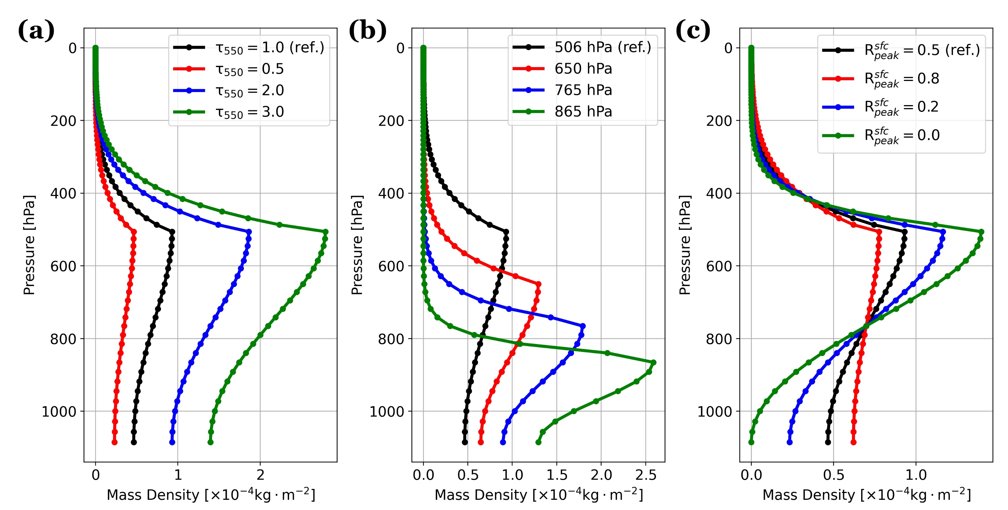
In these sensitivity tests, fourteen GOCART aerosol species used in CRTM were categorized into four types of aerosols, including dust (bin 1 to 5), sea salt (bin 1 to 4), carbonaceous (black and organic carbon), and sulfate aerosols. Instead of using arbitrary profiles, we investigated the aerosol distributions from MERRA-2 and GEOS to build a formulation that generates aerosol profiles similar to model output. In the formulation, an aerosol profile is determined by aerosol loading, peak layer altitude, and the mass density ratio between surface and peak layer () (see Appendix A.1 for details).
For each type of aerosol, we constructed a reference profile to represent the hazy-sky condition. We then perturbed different aspects of the reference profiles, including (1) aerosol mass loading, (2) peak layer altitude, (3) aerosol layer thickness, and (4) bin partition. For the sensitivity tests, we only changed one aspect at a time. Figure 1 shows the reference profile and perturbations for dust aerosols. The reference profile, which has of 1.0 (black line), peaks at 506 hPa, and has a moderate of 0.5. For aerosol loading perturbation (Figure 1a), the half, twice, and triple mass loadings relative to the reference were generated. For peak layer altitude perturbation (Figure 1b), we shifted the peak layer to 650, 765, and 850 hPa, which are all below the reference peak (at 506 hPa). For aerosol layer thickness perturbation (Figure 1c), we produced three other profiles by perturbing the . As a result, these profiles represent cases that range from an elevated confined aerosol layer (small ) to a well-mixed aerosol layer (large ).
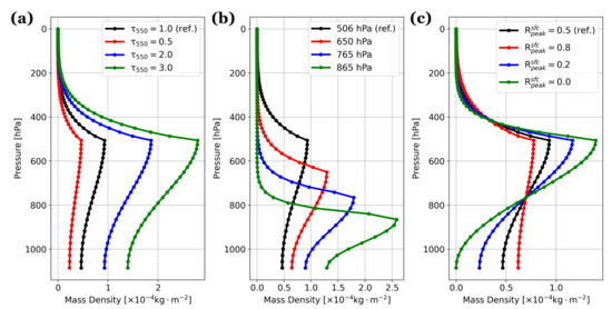
Figure 1.
The profiles for aerosol mass density for the sensitivity tests, including (a) aerosol mass loading, (b) peak layer altitude, and (c) aerosol layer thickness. The reference profile is also labeled in the legends of each panel.
Table 1 lists the bin partition of dust and sea salt aerosols and the composition of carbonaceous and sulfate aerosols. Since the optical properties of each aerosol type are different, we scaled the mass loading of the reference profiles for each aerosol type to generate comparable (∼1.0), which is the standard to measure aerosol loading. As results, the column mass density for reference profiles of dust, sea salt, carbonaceous, and sulfate aerosols corresponds to , , , and , respectively. Note that, for sea salt aerosols, CRTM v2.3 combines the first two sub-micron bins from the GOCART model (which MERRA-2 and GEOS use) into a single fine-mode bin (Lu et al., 2021). It should also be noted that the bin partition is fixed for all layers in all profiles.

Table 1.
The bin partition and composition for the reference profiles of each aerosol type. The corresponding variable names in MERRA-2 are listed.
In addition to the sensitivity tests involving the aerosol profiles, we examined the sensitivity of the bin partition for dust and carbonaceous aerosols to address the different impacts on BTs between a fresh and an aged aerosol plume. Recall, based on the statistics of bin partition from MERRA-2 and GEOS (see Appendix A.1), that their composition changes substantially away from their source regions. For dust, the bin partitions are changed from the values in Table 1 (calculated over West Africa) to 15%, 45%, 35%, 5%, and 0% for DU001–DU005, respectively (calculated over West Atlantic Ocean). The large particles (DU005) are removed essentially at the downwind region. Similarly, for carbonaceous aerosols, the composition is changed to 5%, 90%, 0%, and 5%, where hydrophilic organic carbon predominates. For sea salt, however, it is challenging to separate the source and downwind region, and thus changes in their bin partition were not examined.
3.2. Single IR Observation Experiments
A set of single IR observation experiments using GSI was conducted to demonstrate the impacts of the aerosol-aware BT Jacobians for temperature and water vapor on the analysis. To do this, we conducted an aerosol-blind run (noted as CTL) and an aerosol-aware run (noted as AER) that assimilated a single observation from IASI onboard MetOp-A for the analysis cycle of 12Z 22 June 2020. Among the available channels, we assimilated the IR channel at (∼ ) because the prescribed observation error in GSI is smallest amongst the assimilated IR window channels. Note that the atmospheric states from NCEP GDAS were used as the first guess.
For AER, the time-varying, three-dimensional aerosol information from MERRA-2 was incorporated into the CRTM simulation. That is, the aerosol mixing ratios were spatially and temporally interpolated to the observation location and converted to the mass density for the CRTM simulation. The effective radii for each species at the observation location were determined by the atmospheric states.
To focus on the impact of the aerosol-aware BT Jacobians on the analysis, we had to remove the influence of the BT first-guess departures. Therefore, for both experiments, the first guess was fixed at 5 K and bias corrections on the radiance observations were disabled. To confirm that our results were independent of the first-guess departures, we conducted the same experiment with the departures fixed to 1 K and found that the results were qualitatively similar.
Figure 2 displays the geographic location of the assimilated observation (white mark) and the aerosol column mass density from MERRA-2 over the trans-Atlantic region within the assimilation window (±3 h) for the cycle of 12Z 22 June 2020. Because heavier aerosol loading potentially induces more deviated BT and Jacobians between clear-sky and hazy-sky conditions, we assimilated the observation over ocean at 17.9° N and 60.72° W, which is in the heaviest loading ( > 1.5) of the downwind Saharan dust plume. Moreover, compared to observations over land (such as over the Sahara Desert, which may have larger aerosol loading), observations over ocean are more likely to pass the quality control and be assimilated in GSI because of the smaller uncertainties of surface emissivity.
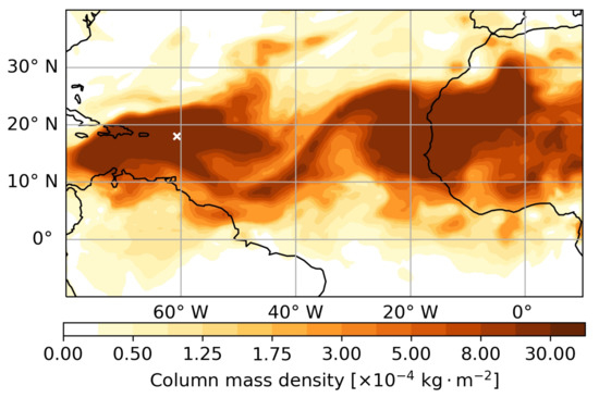
Figure 2.
The column mass density of aerosols of MERRA-2 on 12Z 22 June 2020. The “x” marks the location of the assimilated observation in the single IR observation experiments.
4. Results
4.1. Sensitivity of Simulated BTs
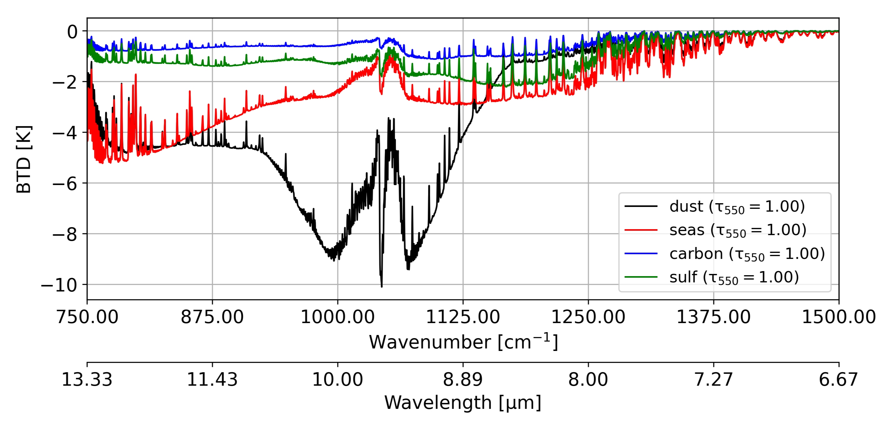
Figure 3 shows the differences between the clear-sky and hazy-sky simulated BTs for the reference profile of the four aerosol types (i.e., different column mass density but the same peak altitude and ). Among the four types, dust aerosols produced the strongest cooling effects in the IR window region. The dust aerosols decreased the BTs up to 10 K at around 1000 to 1100 , while sea salt, carbonaceous, and sulfate aerosols decreased the BTs by around 3 K, 1 K, and 2 K, respectively. This feature of varying cooling effects between aerosol species is consistent with the results reported in Kim et al. [17] and Wei et al. [18]. It should be noted that sea salt aerosols produced comparable BT cooling (∼5 K) to the dust aerosols at around the 750 to 800 region. This is attributed to the larger extinction coefficient of sea salt, which offsets the lower mass density to produce cooling similar to dust. Since dust has the strongest cooling to simulated BT, we next present the sensitivity of CRTM simulations to the dust profiles; results for the other aerosol types are provided in Appendix A.2.
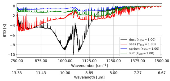
Figure 3.
The brightness temperature differences between clear sky and hazy sky for IASI between 750 to 1500 .
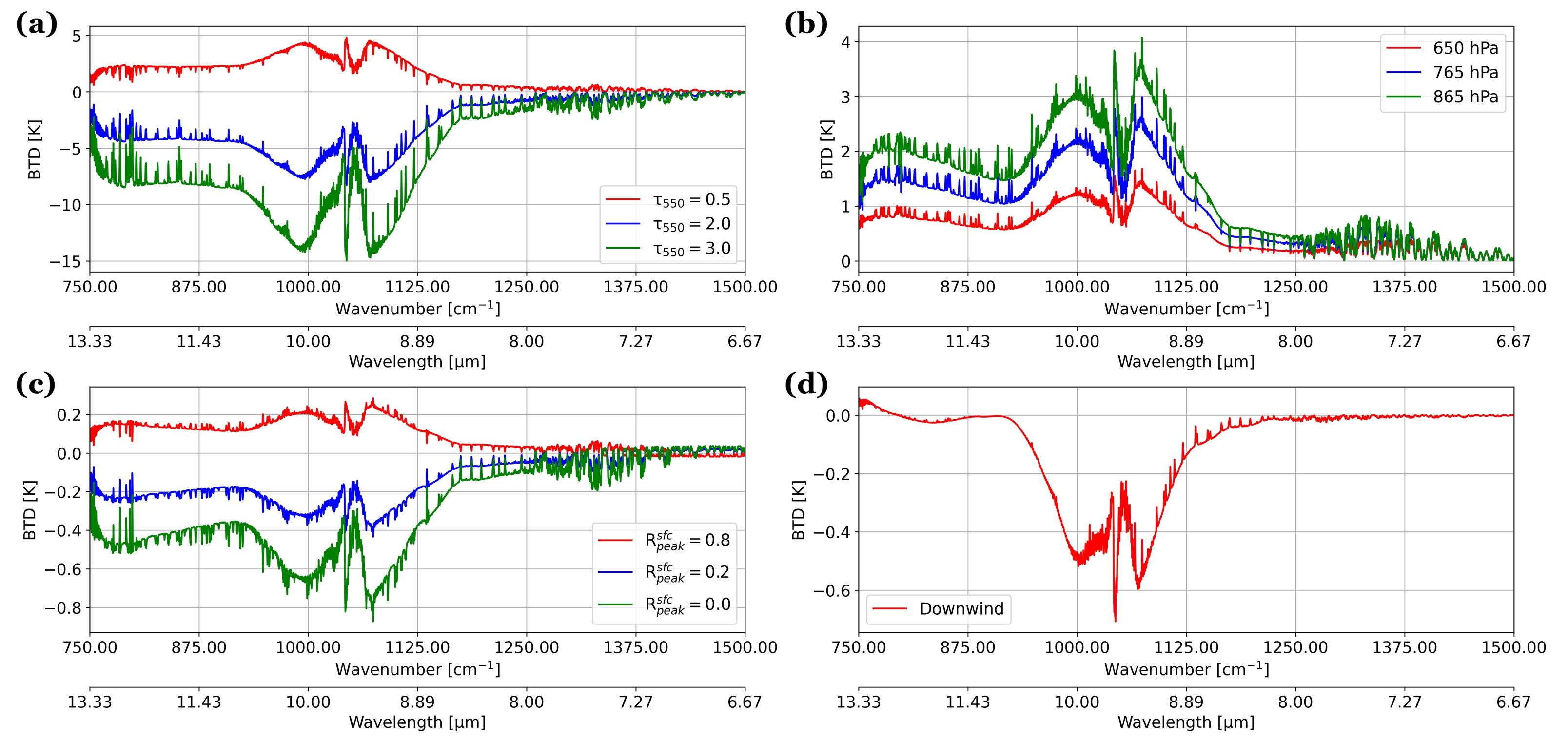
Figure 4 displays the differences between simulated BTs computed from the perturbed profiles and the reference profile for the four sensitivity tests of dust aerosols. For the changes induced by different mass loading, Figure 4a shows that the cooling effect in simulated BTs is weakened by around 5 K when the loading is reduced by half, which translates to roughly half of the BT cooling in the reference case. In contrast, there is an additional 8 K cooling when the loading is doubled and 15 K of cooling when the loading is tripled. This monotonic increase in cooling is expected given the fixed atmospheric states, i.e., the aerosol layer is optically thicker, with larger loading, and thus blocks more IR radiation emitted from the surface.

Figure 4.
The relative change in simulated BT of IASI against the reference dust profile () for each sensitivity test: (a) column mass density, (b) altitude of peak dust layer, (c) thickness, and (d) bins partition.
For the sensitivity to the altitude of the peak dust layer, Figure 4b shows that the magnitude of the cooling effect decreases as the peak layer decreases in altitude. For example, relative to the reference profile that peaks at 506 hPa, the dust layer that peaks at 865 hPa reduces the cooling effect by around 4 K. This implies that the aerosol layer confined to lower levels has smaller impacts on BT, which is consistent with the findings in Pierangelo et al. [10]. This can be attributed to the larger dependencies of the simulated BTs on the aerosol layer temperature. Since our temperature profile warms as altitudes decrease, the case with a lower peak altitude produces a warmer BT.
For the sensitivity to the dust layer thickness, Figure 4c shows that the cooling effect reduces for thicker dust layers with identical mass loading (i.e., = 0.8). When the dust aerosols are more confined to the mid-atmosphere (i.e., = 0.0), the cooling effect is strengthened by around 0.6 K. This indicates that a confined aerosol layer induces a stronger cooling effect on BTs than a well-mixed aerosol layer. This might be attributed to the larger aerosol loading at the peak layer, which can block more IR radiation emitted by the layers below.
For the sensitivity to the bin partition of the dust profile, Figure 4d indicates that the BTs in the IR window region are cooler by approximately 0.7 K for the bin partition representing the downwind region assuming the same mass loading. This implies that more fine-mode particles produce a stronger cooling effect, which is mainly attributed to fine-mode aerosols (i.e., bins 2 and 3) having larger extinction coefficients than other bins for this spectral range (not shown).
Overall, the four sensitivity tests in Figure 4 indicate that the mass loading and the altitude of the peak layer are the primary and secondary factors affecting the simulated BTs, respectively. The changes to the cooling effect due to the thickness and the bin partition of the dust aerosol layer are less than 10% of the cooling effect in the reference case. It also indicates that, under the same aerosol mass loading, a more confined aerosol layer located at higher altitudes would create stronger cooling in simulated BTs. For other aerosol types, the changes in cooling effects relative to their reference profiles show similar features to that shown in Figure 4, including (1) a monotonic increase in the case of mass loading, (2) around 40% reduction in BT cooling when the peak layer altitude changes from 506 to 865 hPa, and (3) around 10% enhanced BT cooling for the most confined aerosol layer (i.e., = 0.0) compared to the reference aerosol layer (i.e., = 0.5).
4.2. Sensitivity of BT Jacobians
In this section, we examine the BT Jacobians for the air temperature (), water vapor (), surface temperature (), and surface emissivity (). To quantify the changes in the and the profiles in the CRTM simulation, the approach in Garand et al. [29] is utilized to calculate the column change rate (defined below). For the and , a direct comparison with the clear-sky simulation is made. The results of are not presented because the calculation of is problematic under multiple-scattering conditions in CRTM v2.3.0. As in Section 4.1, our focus is on the perturbed dust profiles, but results of the sensitivity of BT Jacobians for the other aerosols are shown in Appendix A.2.
The column change rate (M) value for the Jacobian of interest is calculated as follows:
where is the Jacobian profile to evaluate, is the reference Jacobian profile, and the superscript l is the vertical layer. The uses the Jacobian from the clear-sky simulation. The M represents the total column rate of change for the Jacobian of interest.
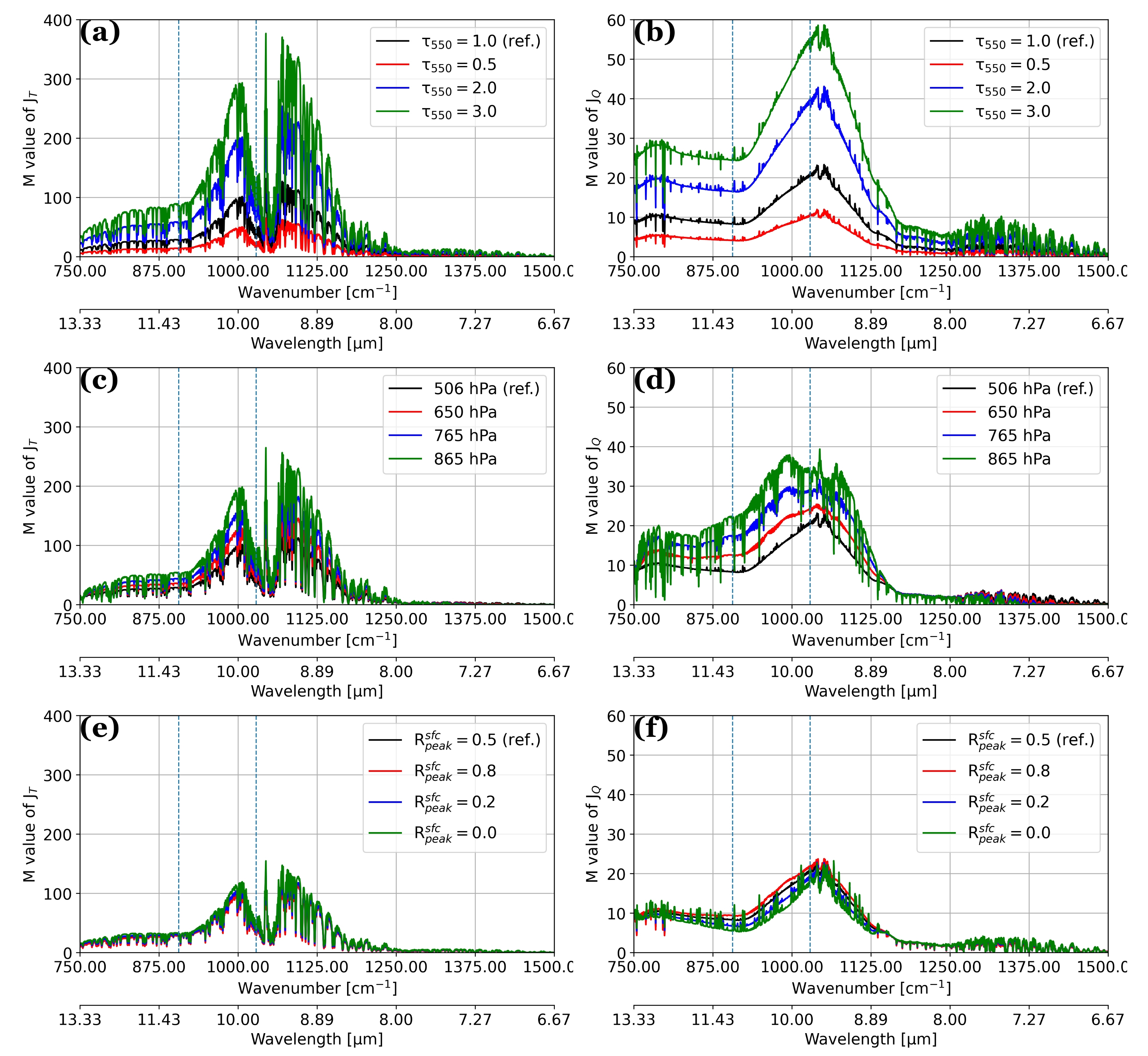
Figure 5 illustrates the M values of and in the IR window region from the same set of dust sensitivity tests shown in Figure 4. We exclude the results from the bin partitions, however, because the differences are negligible. The reference dust profile (black line) produces approximately 100 and 20 of M values in and , respectively. This means that is more sensitive to considering aerosol transmittance effects in BT simulations than .
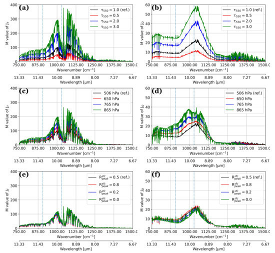
Figure 5.
The column change rate of Jacobians for layer temperature (, left column) and layer water vapor (, right column) from sensitivity tests in (a,b) column mass density, (c,d) altitude of peak dust layer, and (e,f) thickness. The two selected channels for vertical distribution in Figure 6 are marked by dashed lines.
Similar to the results of the simulated BTs, the M values of and are most sensitive to the changes in mass loading (Figure 5a,b) and peak layer altitude (Figure 5c,d). The dust profiles that have triple the reference loading and that peak at 865 hPa introduce the largest changes in and . Regarding the sensitivity to the dust layer thickness (Figure 5e,f), the M values of the and the show smaller differences between different layer thicknesses compared to the tests for mass loading and peak layer altitude. This could be attributed to the minimal change in the layer mass loading for our different dust layer thickness profiles (Figure 1c). However, a larger mass loading at a more confined layer could induce larger changes in the and the .
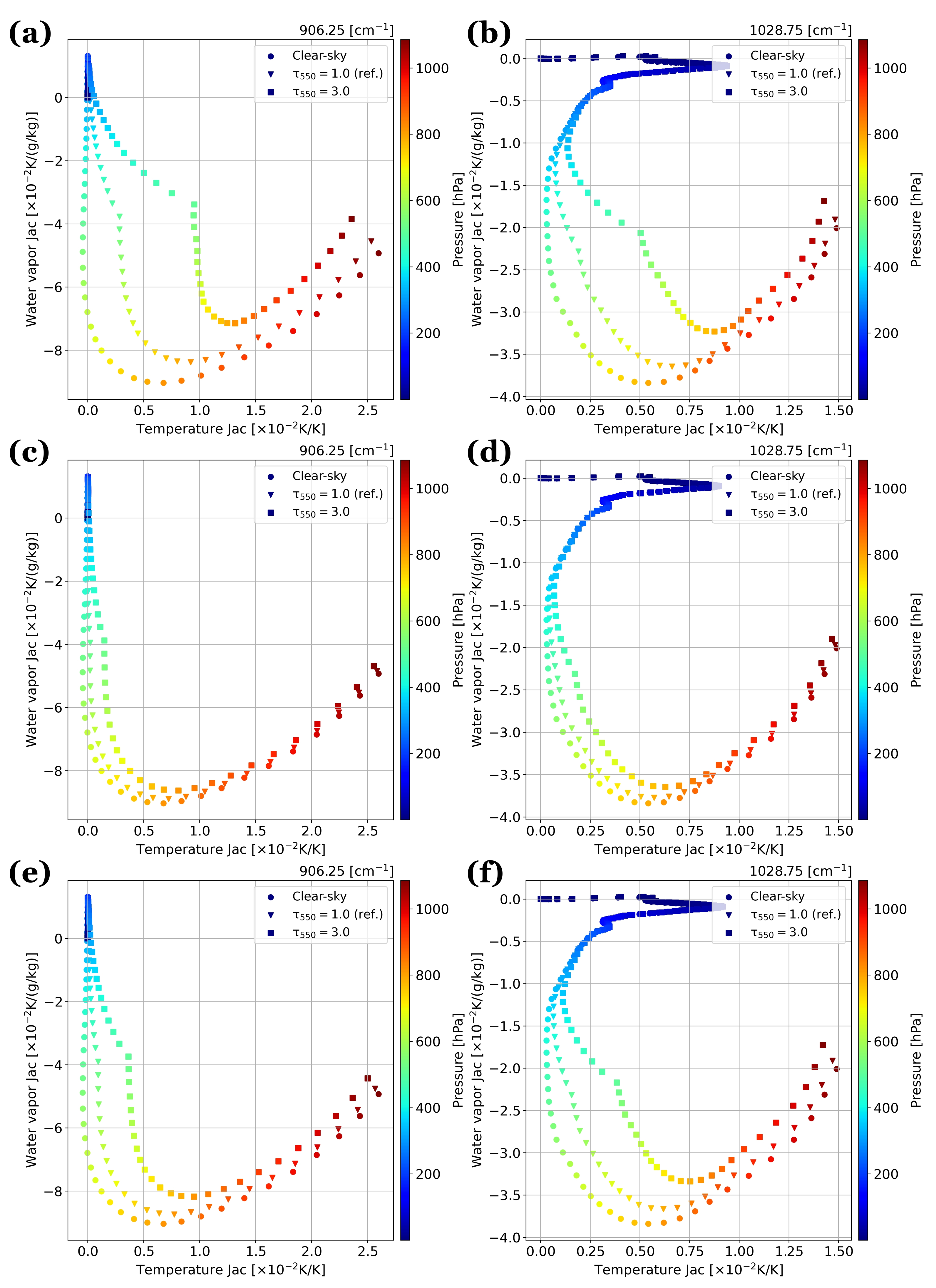
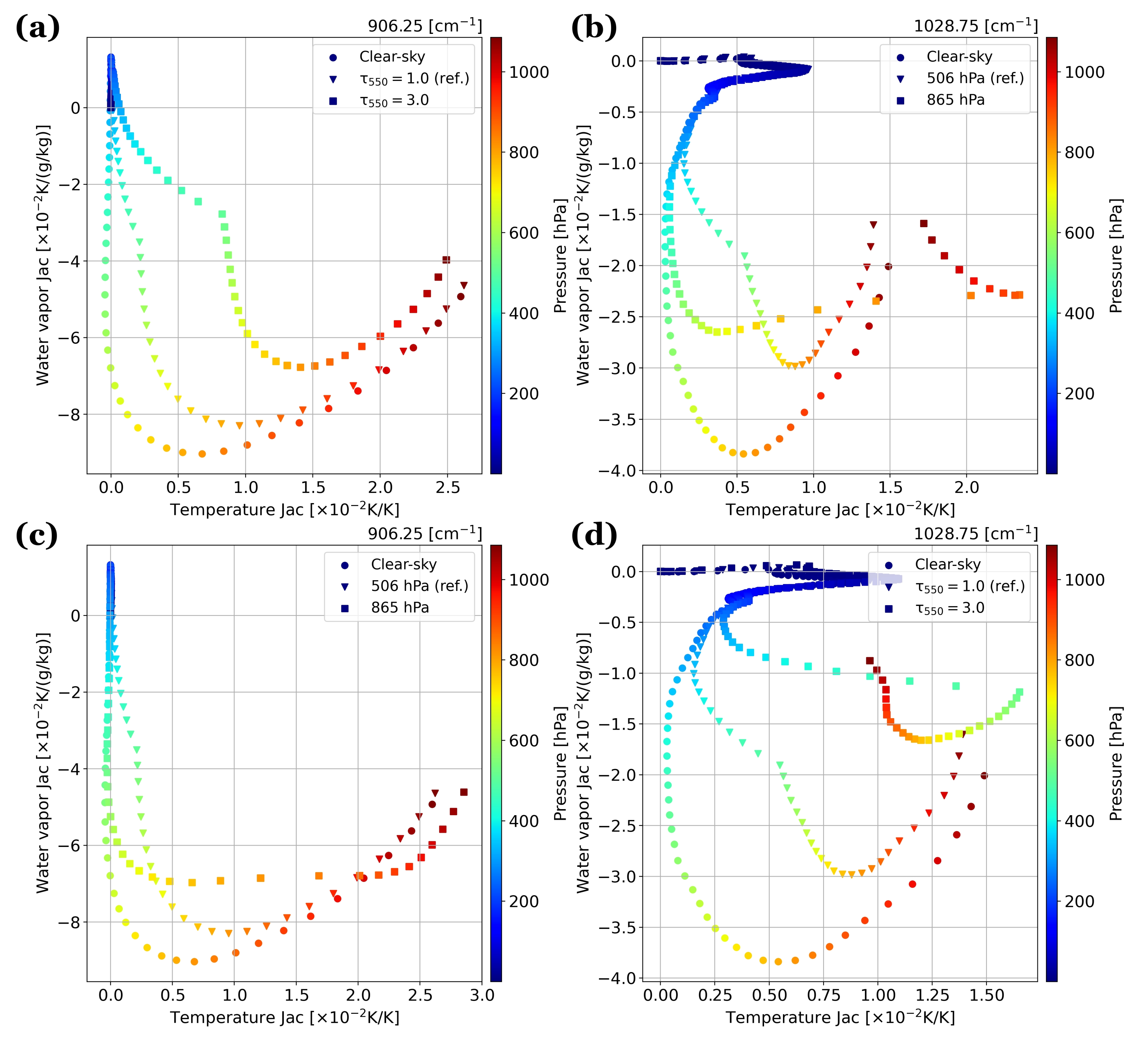
To demonstrate the impacts of aerosols on the vertical distribution of and , we select two IR channels from IASI, and , which are located in the window region and ozone absorption line, respectively. In GSI, these channels have relatively small observation error compared to the other channels assimilated in the similar spectral range. Given the small observation error, assimilating these two channels will be more impactful to the analyses.
Figure 6 displays vertical changes in the Jacobians to the (a, b) dust loading and (c, d) peak altitude at the two channels. In Figure 6, each layer of in the x-axis and in the y-axis is plotted as dots of a different color. For the clear-sky case (circles), the at is small above 600 hPa and monotonically increases to the surface, while at the locally peaks in the stratosphere due to ozone absorption, relaxes back in the middle atmosphere (∼500 hPa), and then peaks at the surface. Meanwhile, at both channels, the for the clear-sky case is slightly positive in the upper atmosphere and peaks around 800 hPa.

Figure 6.
The scatter plots of Jacobians for layer temperature (in x) and layer water vapor (in y) from the two assimilated IR window channels: (left column) and (right column). The sensitivity tests of (a,b) column mass density and (c,d) peak altitude are shown. Clear sky is in ●; reference is in ▼ and triple loading 865 hPa peaks are in ■. Color of dots represents the layer pressure.
Compared to the clear-sky case (circles), the reference dust loading (triangles) increases the magnitude of at below 400 hPa, where the dust loading is high (see black line in Figure 1). Similarly, at , the reference dust loading increases the below 400 hPa, but slightly decreases the at the lowest few layers. The triple loading (squares) creates stronger changes to but decreases the in the lowest few layers at (Figure 6a), while it shows different behavior at (Figure 6b; discussed below). At both channels, the for the two different dust loadings has smaller magnitudes than the clear-sky case in most layers affected by dust. For instance, at , the near 500 hPa is approximately −4, −3.5, and −2.8 K/(g/kg) for the clear-sky (), reference (), and triple loading (), respectively. Figure 6c,d illustrate the changes in and due to the peak altitude of the dust layer. Compared with the reference profile (triangles), the of the lower peak altitude profile (squares) always increases within the aerosol layer but it also shows a different behavior at (Figure 6d; discussed below). For the magnitude of , it is always smaller than the reference and near constant above the peak layer (865 hPa), while it decreases substantially below the peak at both channels. These features imply that the aerosol-affected simulated BTs are more sensitive to the temperature of the aerosol layer and less sensitive to water vapor.
As mentioned above, there is a different behavior of under the conditions of heavy dust loading ( = 3.0) and lower peaking altitude (865 hPa) at , which indicates the changes in peak levels in (Figure 6b,d). For these two cases, the peaks at a similar altitude at which the dust layer has the largest loading (506 and 865 hPa) and reduces in the layers below. In contrast, the other two cases (clear-sky and reference) show the peaks at the lowest layer. This change to the peak of the means that the dust layers in both cases block most IR radiation emitted from the surface and the layers below the peak. It suggests that the simulated BTs become the most sensitive to the temperature of the aerosol layer instead of the surface when an optically thick aerosol plume is aloft. Consequently, assimilating a hazy-sky observation as a clear-sky observation (i.e., without considering aerosol information) could introduce errors into the magnitude and the vertical distribution of the analysis increment via BT differences and Jacobians.
Regarding the , Figure 7 displays the comparison of between the clear-sky and reference dust profile and the sensitivity of to the different aerosol mass loadings. The differences in other sensitivity tests are not as pronounced and are thus excluded. Figure 7a indicates that the is smaller when considering the dust aerosols. Figure 7b depicts that the decreased by around 20% in the reference case and up to around 50% when was 3.0. This implies that the simulated BTs are less sensitive to the surface temperature when more surface-emitted IR radiation is attenuated by the aerosol layer with larger mass loading. The smaller and cooler simulated BTs under the hazy-sky condition conjunctively enlarge the “skin temperature sensitivity related parameter” employed in the QC algorithm of GSI [19] and thus can lead to more IR observations rejected due to this QC check, as reported in Wei et al. [18].
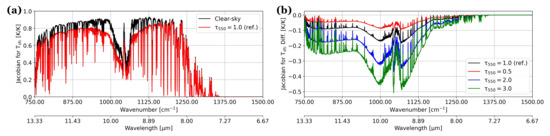
Figure 7.
(a) The comparison of the Jacobian for surface temperature () between clear-sky (black) and reference dust profile (red) and the (b) relative changes due to the perturbed column mass density.
4.3. Single IR observation Test
In this section, the results from CTL and AER are presented (see Section 3.2). Recall that, for both experiments, the first-guess departure is fixed to focus on the aerosol-affected BT jacobians on the analysis increments. For this scenario, both experiments use the same , , and in Equation (1). Therefore, the more positive , as observed in Section 4.2, will generate a more positive temperature increment because it maps a larger B to BT space. Similarly, the less negative will generate a less negative water vapor increment. It assumes that the analysis increments of a given variable are influenced solely by the Jacobians of the same variable, i.e., the only affects the analysis increment for temperature. However, in reality, the influence of the Jacobians on the increments is not a one-to-one relationship, which will be demonstrated below.
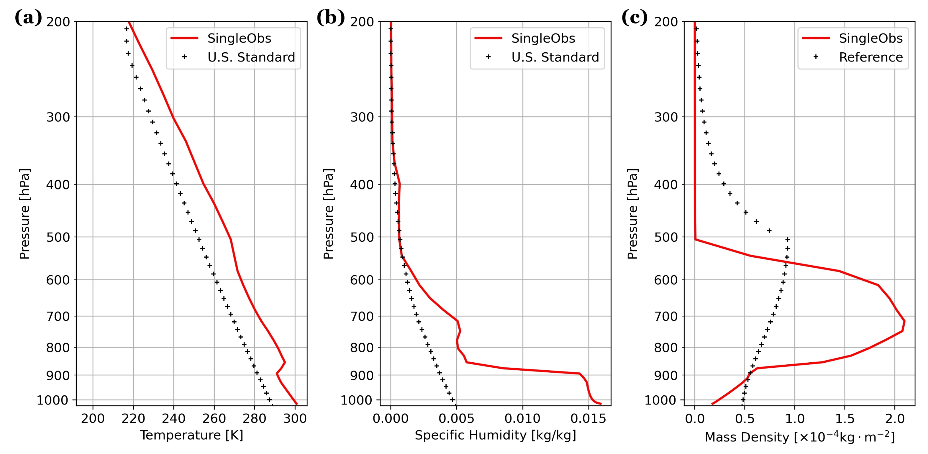
Figure 8 shows the vertical profiles of temperature, specific humidity, and aerosol mass density at the observation for our experiments (red; see Figure 2 for location) and the CRTM sensitivity tests (black dots). Compared with the U.S. standard atmosphere used in our CRTM sensitivity tests, the profiles of temperature and specific humidity (Figure 8a,b) show a warmer and more moist atmosphere, respectively. The profiles also capture the trade wind inversion, from 900 to 850 hPa, which is below the dry Saharan Air Layer (SAL), from 850 to 600 hPa [30]. As expected, the aerosol profile (Figure 8c) is elevated over the marine layer and distributed throughout the SAL, from 950 to 650 hPa.
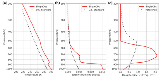
Figure 8.
The vertical profiles of (a) temperature, (b) specific humidity, and (c) aerosol mass density for the observation at 17.9° N and 60.7° W.
Figure 9 displays the BT Jacobians for the virtual temperature () and moisture variable () at the observation. In general, both (Figure 9a) and (Figure 9b) have similar aerosol-induced responses to the results of the CRTM sensitivity tests shown in Section 4.2. That is, with aerosols, is more positive within the aerosol layer and is less negative. However, in contrast to the CRTM sensitivity tests, the of both experiments in Figure 9a peaks at around 900 hPa instead of at the lowest model level. This feature, which is not affected by the aerosols, is likely attributed to the different ambient conditions (e.g., the temperature inversion and higher water vapor content shown in Figure 8).
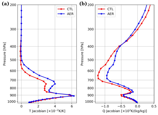
Figure 9.
BT Jacobians for (a) layer virtual temperature and (b) moisture for at the observation. Note that the magnitude of (b) is different to Figure 6 because of the unit conversion in GSI.
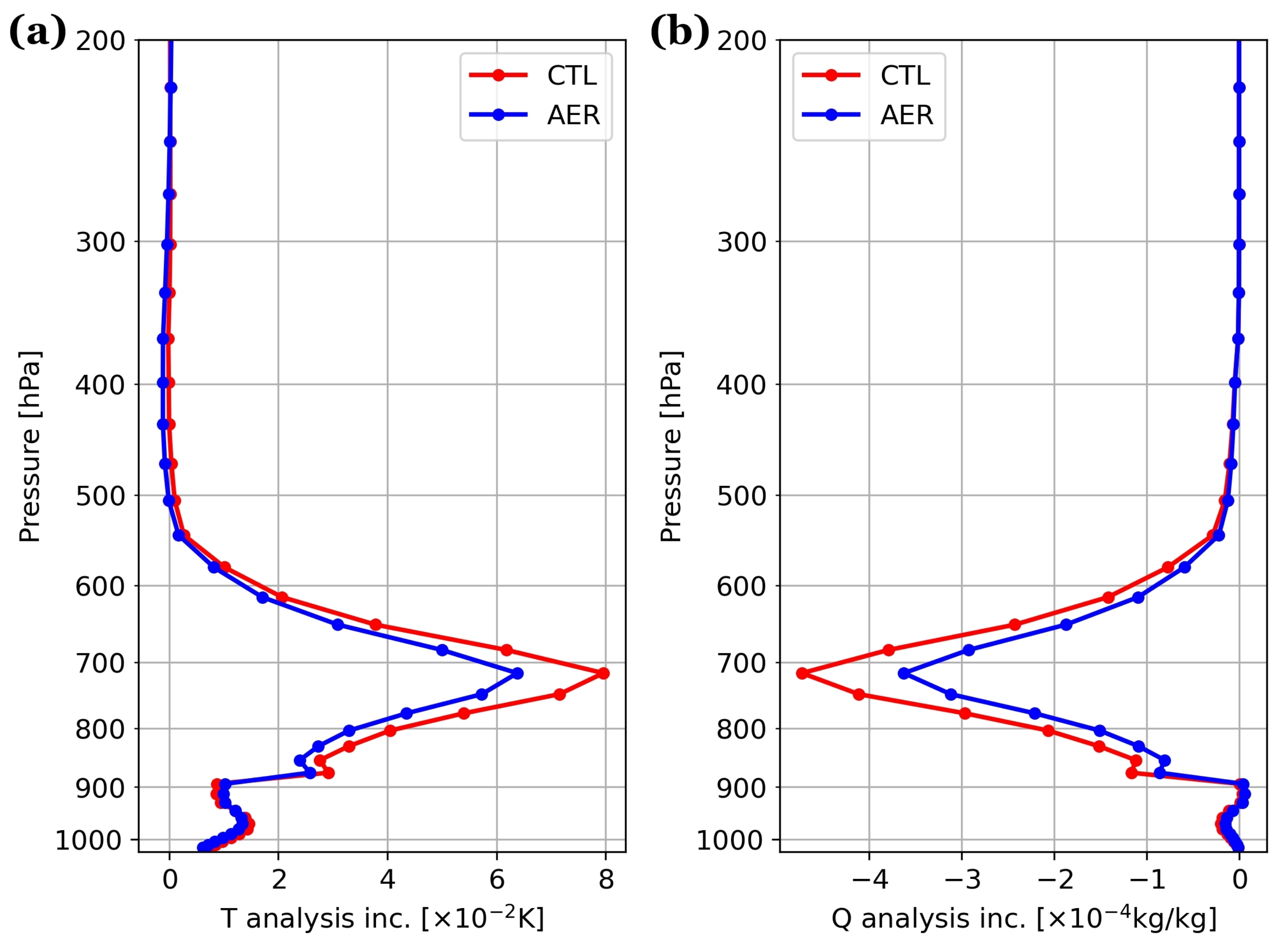
Figure 10 shows the analysis increments on the temperature and specific humidity for the single observation experiment. Compared to clear-sky Jacobians (i.e., CTL), the changes induced by aerosol-affected Jacobians (i.e., AER) on the increments are largest (∼25% of CTL) where the Jacobians are also most deviated, i.e., between 600 and 800 hPa. In this region, the relative changes are more impactful to specific humidity, which is around 2% of the first-guess value (cf. 0.0001 kg/kg vs. 0.005 kg/kg) while the changes in temperature are only approximately 0.004% (cf. 0.01 K vs. 280 K). AER generates a less positive temperature increment and less negative specific humidity increment. This means that the atmospheric analysis is cooler and more humid. The influence of the aerosols on the temperature increment, however, is not the same as expected from Equation (1), where a more positive temperature Jacobian would produce a more positive analysis temperature increment. Rather, the results from Figure 10 suggest that the analysis increments of a given variable are affected by the aerosol-induced changes to all of the atmospheric Jacobians in GSI (i.e., both and ).

Figure 10.
The analysis increments of (a) layer temperature and (b) specific humidity at the observation.
To clarify the response in the analysis increments, two additional sets of single IR observation experiments (not shown) were conducted to identify the contribution from the and the to the analysis increments. In GSI, CRTM-derived Jacobians for surface wind, sea surface temperature, air temperature, water vapor mixing ratio, and ozone are utilized during the minimization. Hence, we conducted one experiment where the analysis increments were determined solely by the Jacobian for virtual temperature (-only) and another experiment with the same configuration but the analysis increments were determined solely by the Jacobian for water vapor (-only). In the case of only, the temperature increments in AER become more positive than in CTL at the levels where the was more positive, as expected from Equation (1). On the other hand, for the only case, it produced similar temperature and specific humidity increments in Figure 10. Therefore, the changes to the analysis increments by the aerosols are attributed to the complexity of the Jacobians’ influence, which has a multivariate relationship between the temperature and moisture fields controlled by the moisture analysis variable [31].
5. Discussion and Conclusions
In this study, we examined (i) how the simulated BTs and Jacobians respond to the characteristics of aerosol profiles and (ii) how these aerosol-induced changes in atmospheric Jacobians influence the analysis. To do this, we conducted two experiments focusing on the IR window region. First, we performed a series of CRTM sensitivity tests with aerosol profiles that were perturbed from loading, peak altitude, thickness, and bin partition. Second, we ran GSI single IR observation experiments that assimilated an IR window channel observation over the trans-Atlantic region with and without considering aerosol transmittance effects in CRTM. Both experiments were performed with the Infrared Atmospheric Sounding Interferometer (IASI), which is a high-spectral-resolution IR sensor. The findings here, however, can be applied to other IR sensors assimilated in DA systems, such as the Cross-track Infrared Sounder (CrIS) and Atmospheric Infrared Sounder (AIRS).
In the present study, the key findings from the CRTM sensitivity and single IR observation experiments are:
- Dust aerosols generate stronger impacts on BTs than other species (Figure 3). For other aerosol species, their influences could be limited on BTs due to the relatively smaller particle size and extinction coefficients.
- An aerosol layer with heavier loading that peaks at higher altitude can produce the strongest cooling to simulated BTs (Figure 4). In contrast, the thickness and the bin partition of an aerosol layer provide smaller influences on simulated BTs.
- The aerosol-induced differences in atmospheric Jacobians produce considerable changes (∼25%) to analysis increments for specific humidity and temperature (Figure 10). In particular, the changes to the analysis increment for temperature are largely controlled by the water vapor Jacobian, which begins to unravel the complexity of how atmospheric Jacobians affect the analysis.
These key findings provide guidance toward an aerosol-aware DA system, especially for aerosol-aware QC and BC [18]. For aerosol-aware QC, the smaller Jacobian for surface temperature implies that the existing quality control (QC) check involving the “skin temperature sensitivity related parameter” can be relaxed or omitted for observations under hazy-sky conditions. For aerosol-aware BC, the large sensitivity to aerosol loading and peak altitude reveals that model biases on these two factors should be addressed in the bias correction (BC) algorithm. The aerosol impact on the Jacobian for surface emissivity, however, is not determined in this study. This is because of the problematic calculation under scattering conditions in the version of CRTM, which caused considerable changes in the BC algorithm [18]. The problem has been resolved in the newer version of CRTM.
There are, however, several limitations on our CRTM sensitivity tests that require further study. These include (i) the assumption of particle size distribution, (ii) optical properties for aerosols, and (iii) fixed ambient conditions. Prior studies have reported that different assumptions of particle size distribution [32] and different sets of optical properties and atmospheric states [33] can also introduce perturbations to the radiance simulation. Moreover, we found differences in the aerosol-affected Jacobians between the reference CRTM sensitivity test and the single IR observation experiments (see Figure 9), which we attributed to the differences in the environment (see Figure 8). Therefore, a more extensive study is desired to investigate the aerosol-affected BT simulations under various atmospheric conditions and optical properties, especially within dust-laden regions.
In summary, a DA system that does not constrain aerosol transmittance effects can introduce inaccurate cooling to the analyzed temperature due to warm biases in simulated BTs and inaccurate increments to the analyzed moisture variable when aerosol-affected observations are assimilated as clear-sky observations. These issues will be more critical over dust-laden regions, such as North Africa and the trans-Atlantic during summer, because of the high loading from Saharan dust. Consequently, the errors in analysis for both temperature and water vapor may degrade the forecasts of the African easterly waves and thus the tropical storm activities [34]. However, a DA system constraining the aerosol transmittance effects in IR radiance simulations by incorporating modeled aerosols is a feasible solution [17,18]. Based on the uncertainties in IR radiance simulations due to aerosols realized in this study, a future study using the latest CRTM that implements the QC checks and the BC predictors for assimilating hazy-sky IR observations is desired to investigate its impacts on analyses and forecasts.
Author Contributions
Conceptualization, S.-W.W. and C.-H.L.; methodology, S.-W.W. and C.-H.L.; software and visualization, S.-W.W.; validation, S.-W.W.; investigation, S.-W.W., C.-H.L., B.T.J., C.D., P.S., D.G., G.G. and M.H.; writing—original draft preparation, S.-W.W.; writing—review and editing, S.-W.W., C.-H.L. and D.G.; supervision, C.-H.L.; project administration, C.-H.L.; funding acquisition, C.-H.L. All authors have read and agreed to the published version of the manuscript.
Funding
This research is supported by the Climate Program Office (CPO) Modeling, Analysis, Predictions and Projections (MAPP) within NOAA/OAR (award number NA18OAR4310282).
Institutional Review Board Statement
Not applicable.
Informed Consent Statement
Not applicable.
Data Availability Statement
The data that supports the findings of this study is archived at NESDIS- funded Supercomputer for Satellite Simulations and Data Assimilation Studies (S4) cluster and can be made available to the readers upon request.
Acknowledgments
All code development and experiments were conducted on Hera, an R&D high-performance computing system (RDHPCS) at the NOAA Environmental Security Computing Center (NESCC). Guoqing Ge was supported in part by the NOAA Cooperative Agreement with CIRES, NA17OAR4320101.
Conflicts of Interest
The authors declare no conflict of interest.
Appendix A
Appendix A.1. Determination of Aerosol Mass Density Profile
The vertical profiles of each aerosol type are determined by the altitude of the peak layer, the ratio of accumulated loading below and above the peak aerosol layer, the ratio of loading at the peak layer and the lowest layer (), and bin partition. These variables are generated based on the statistics of dust aerosols in the summer months (June, July, and August) of the MERRA-2 2003-2014 climatology and episodic plumes for four types (defined in text) of aerosols in GEOS forward processing (FP) of June and September 2020. To reduce the complexity, the ratio of accumulated loading below and above the peak aerosol layer is fixed at 4 (cf. 80% below vs. 20% above), which is the median number within aerosol plumes. The equation for the mass density profile () is
where C is the total mass density, k is the layer index in CRTM simulation (k = 1∼100), and p is the layer index of peak aerosol loading. Given C, the steps to construct the aerosol profiles are as follows:
- Assign the altitude of the peak layer (506 hPa for the reference).
- Place 20% of the mass loading above the peak layer () and 80% () at and below the peak layer (this ratio is fixed for all aerosol profiles).
- Distribute the 80% at and below the peak layer based on a cosine function ( at peak to at surface) and the Rsfcpeak (0.5 for the reference profile), which determines the aerosol layer thickness.
- Distribute the 20% above the peak layer to exponentially decay with height. The decaying ratio is , where is the mass density at the peak layer.
- Distribute the loading at each layer to the bins for each type of aerosol based on the bin partition.
Appendix A.2. Results of Sensitivity Tests for Other Aerosol Types
Figure A1 shows the differences between simulated BTs computed from the perturbed profiles and the reference profile for the other three aerosol types (i.e., sea salt, carbonaceous, and sulfate). As presented in Section 4.1, the results have similar features to dust aerosols. Moreover, it shows the different spectral signatures of BTs among aerosol types: the changes to the BT differences for sea salt, carbonaceous, and sulfate aerosols are largest near 800 , 1100 , and 1175 , respectively.
Figure A2 shows the column change rate (M; defined in Section 4.2) of Jacobians for temperature and water vapor from the other three aerosol types. Here, we present the sensitivity tests of aerosol loading, which have more discernible differences among different conditions. The M values reflect the BT differences shown in Figure 3. For instance, the larger BT differences of sea salt aerosols lead to stronger changes in and compared to sulfate and carbonaceous aerosols. The M values also show that the sea salt aerosols result in a comparable change rate to and at the region smaller than 900 , where sea salt and dust aerosols have similar BT differences.
Figure A3 displays the scatter plots of and from aerosol loading tests for sea salt, carbonaceous, and sulfate aerosols. Among these three aerosol types, sea salt aerosols show the most deviated and from clear sky. The differences between three conditions of each aerosol type reflect their cooling effects to BTs. For example, sea salt has comparable magnitude of and to the dust aerosols at , where sea salt and dust have similar cooling effects to BTs. In contrast, at , the magnitude of and in the tests of sea salt is smaller than dust aerosols, which is where the cooling effects to BTs induced by sea salt is also small (Figure 3).
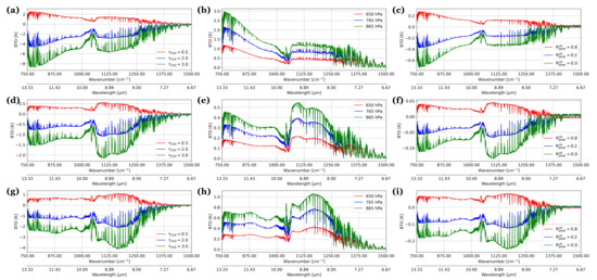
Figure A1.
The relative change in simulated BT of IASI against the reference profile () of (a–c) sea salt, (d–f) carbonaceous, and (g–i) sulfate aerosols. Columns from left to right are the results from sensitivity tests of aerosol loading, peak altitude, and thickness, respectively.
Figure A1.
The relative change in simulated BT of IASI against the reference profile () of (a–c) sea salt, (d–f) carbonaceous, and (g–i) sulfate aerosols. Columns from left to right are the results from sensitivity tests of aerosol loading, peak altitude, and thickness, respectively.
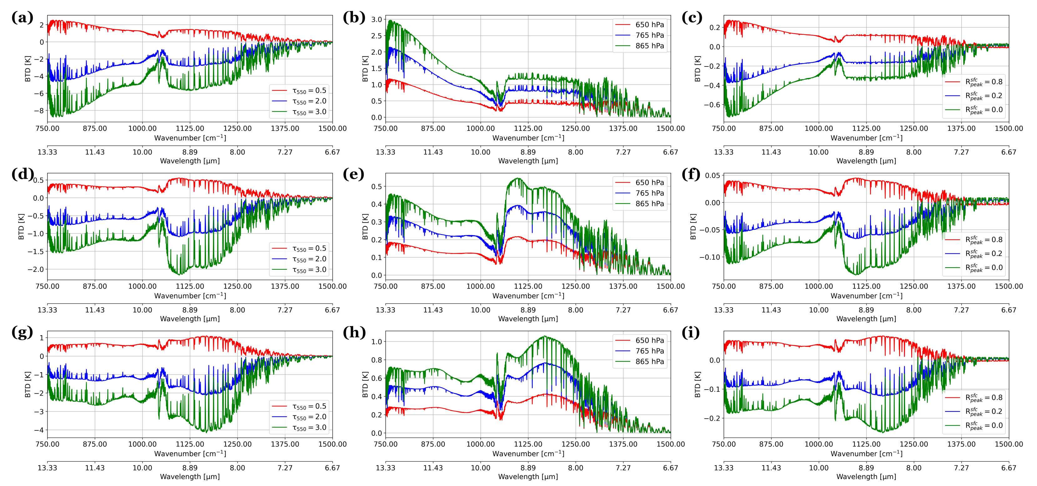
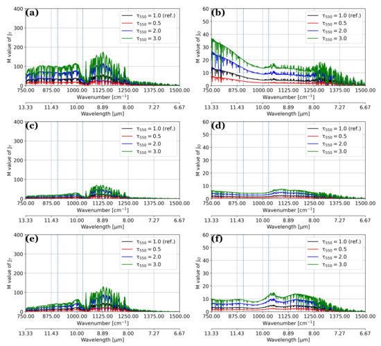
Figure A2.
The column change rate (M) of Jacobians for temperature (left column) and water vapor (right column) from the aerosol loading sensitivity tests for (a,b) sea salt, (c,d) carbonaceous, and (e,f) sulfate aerosols.
Figure A2.
The column change rate (M) of Jacobians for temperature (left column) and water vapor (right column) from the aerosol loading sensitivity tests for (a,b) sea salt, (c,d) carbonaceous, and (e,f) sulfate aerosols.
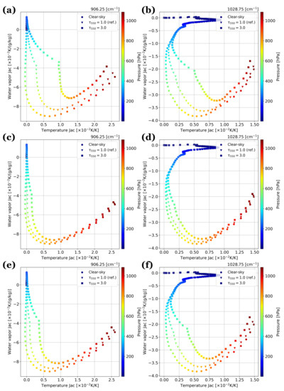
Figure A3.
The scatter plots of Jacobians for layer temperature (in x) and layer water vapor (in y) from the two assimilated IR window channels, (left column) and (right column). The sensitivity tests of column mass density are shown for (a,b) sea salt, (c,d) carbonaceous, and (e,f) sulfate aerosols. Clear sky is in ●, reference is in ▼, and triple loading is in ■. Color of dots represents the layer pressure.
References
- Courtier, P.; Andersson, E.; Heckley, W.A.; Kelly, G.; Pailleux, J.; Rabier, F.; Thepaut, J.N.; Unden, P.; Vasiljevic, D.; Cardinali, C.; et al. Variational Assimilation at ECMWF; ECMWF Technical Memoranda; European Centre for Medium Range Weather Forecasts: Reading, UK, 1993; Volume 194. [Google Scholar]
- Eyre, J.R.; Kelly, G.A.; McNally, A.P.; Andersson, E.; Persson, A. Assimilation of TOVS Radiance Information through One-Dimensional Variational Analysis. Q. J. R. Meteorol. Soc. 1993, 119, 1427–1463. [Google Scholar] [CrossRef]
- Andersson, E.; Pailleux, J.; Thépaut, J.-N.; Eyre, J.R.; McNally, A.P.; Kelly, G.A.; Courtier, P. Use of Cloud-Cleared Radiances in Three/Four-Dimensional Variational Data Assimilation. Q. J. R. Meteorol. Soc. 1994, 120, 627–653. [Google Scholar] [CrossRef]
- Derber, J.C.; Wu, W.-S. The Use of TOVS Cloud-Cleared Radiances in the NCEP SSI Analysis System. Mon. Wea. Rev. 1998, 126, 2287–2299. [Google Scholar] [CrossRef]
- Courtier, P.; Andersson, E.; Heckley, W.; Vasiljevic, D.; Hamrud, M.; Hollingsworth, A.; Rabier, F.; Fisher, M.; Pailleux, J. The ECMWF Implementation of Three-Dimensional Variational Assimilation (3D-Var). I: Formulation. Q. J. R. Meteorol. Soc. 1998, 124, 1783–1807. [Google Scholar] [CrossRef]
- Saunders, R.; Hocking, J.; Turner, E.; Rayer, P.; Rundle, D.; Brunel, P.; Vidot, J.; Roquet, P.; Matricardi, M.; Geer, A.; et al. An Update on the RTTOV Fast Radiative Transfer Model (Currently at Version 12). Geosci. Model Dev. 2018, 11, 2717–2737. [Google Scholar] [CrossRef] [Green Version]
- Weng, F.; Han, Y.; van Delst, P.; Liu, Q.; Kleespies, T.; Yan, B.; Marshall, J.L. JCSDA Community Radiative Transfer Model (CRTM). In Proceedings of the 14th International TOVS Study Conference, BeiJing, China, 25–31 May 2005; p. 6. [Google Scholar]
- Han, Y.; van Delst, P.; Liu, Q.; Weng, F.; Yan, B.; Treadon, R.; Derber, J. JCSDA Community Radiative Transfer Model (CRTM)—Version 1; NOAA Technical Report NESDIS; National Oceanic and Atmospheric Administration National Environmental Satellite, Data, and Information Service: Washington, DC, USA, 2006; Volume 122. [Google Scholar]
- Sokolik, I.N. The spectral radiative signature of wind-blown mineral dust: Implications for remote sensing in the thermal IR region. Geophys. Res. Lett. 2002, 29, 7-1–7-4. [Google Scholar] [CrossRef] [Green Version]
- Pierangelo, C.; Chedin, A.; Heilliette, S.; Jacquinet-Husson, N.; Armante, R. Dust altitude and infrared optical depth from AIRS. Atmos. Chem. Phys. 2004, 4, 1813–1822. [Google Scholar] [CrossRef] [Green Version]
- Matricardi, M. The Inclusion of Aerosols and Clouds in RTIASI, the ECMWF Fast Radiative Transfer Model for the Infrared Atmospheric Sounding Interferometer; ECMWF Technical Memoranda; European Centre for Medium Range Weather Forecasts: Reading, UK, 2005; Volume 474. [Google Scholar]
- Quan, X.; Huang, H.-L.; Zhang, L.; Weisz, E.; Cao, X. Sensitive detection of aerosol effect on simulated IASI spectral radiance. J. Quant. Spectrosc. Radiat. Transf. 2013, 122, 214–232. [Google Scholar] [CrossRef]
- Hess, M.; Koepke, P.; Schult, I. Optical Properties of Aerosols and Clouds: The Software Package OPAC. Bull. Am. Meteorol. Soc. 1998, 79, 831–844. [Google Scholar] [CrossRef]
- Liu, Q.; Han, Y.; van Delst, P.; Weng, F. Modeling aerosol radiance for NCEP data assimilation. In Fourier Transform Spectroscopy/Hyperspectral Imaging and Sounding of the Environment; HThA5; Optical Society of America: Washington, DC, USA, 2007. [Google Scholar] [CrossRef]
- Chen, Y.; Han, Y.; Weng, F. Comparison of two transmittance algorithms in the community radiative transfer model: Application to AVHRR. J. Geophys. Res. Atmos. 2012, 117, D06206. [Google Scholar] [CrossRef] [Green Version]
- Weaver, C.J.; Joiner, J.; Ginoux, P. Mineral aerosol contamination of TIROS Operational Vertical Sounder (TOVS) temperature and moisture retrievals. J. Geophys. Res. 2003, 108, 4246. [Google Scholar] [CrossRef] [Green Version]
- Kim, J.; Akella, S.; da Silva, A.M.; Todling, R.; McCarty, W. Preliminary Evaluation of Influence of Aerosols on the Simulation of Brightness Temperature in the NASA’s Goddard Earth Observing System Atmospheric Data Assimilation System; Technical Report Series on Global Modeling and Data Assimilation; Goddard Space Flight Center; National Aeronautics and Space Administration: Greenbelt, MD, USA, 2018. [Google Scholar]
- Wei, S.-W.; Lu, C.-H.; Liu, Q.; Collard, A.; Zhu, T.; Grogan, D.; Li, X.; Wang, J.; Grumbine, R.; Bhattacharjee, P.S. The Impact of Aerosols on Satellite Radiance Data Assimilation Using NCEP Global Data Assimilation System. Atmos. 2021, 12, 432. [Google Scholar] [CrossRef]
- Liang, D.; Weng, F. Evaluation of the Impact of a New Quality Control Method on Assimilation of CrIS Data in HWRF-GSI. In Proceedings of the 2014 IEEE Geoscience and Remote Sensing Symposium, Quebec City, QC, Canada, 13–18 July 2014; pp. 3778–3781. [Google Scholar]
- Zhu, Y.; Derber, J.; Collard, A.; Dee, D.; Treadon, R.; Gayno, G.; Jung, J.A. Enhanced radiance bias correction in the National Centers for Environmental Prediction’s Gridpoint Statistical Interpolation data assimilation system: Radiance Bias Correction in GSI. Q. J. R. Meteorol. Soc. 2014, 140, 1479–1492. [Google Scholar] [CrossRef]
- Wu, W.-S.; Purser, R.J.; Parrish, D.F. Three-Dimensional Variational Analysis with Spatially Inhomogeneous Covariances. Mon. Wea. Rev. 2002, 130, 2905–2916. [Google Scholar] [CrossRef] [Green Version]
- Liu, Q.; Weng, F. Advanced Doubling—Adding Method for Radiative Transfer in Planetary Atmospheres. J. Atmos. Sci. 2006, 63, 3459–3465. [Google Scholar] [CrossRef]
- Chin, M.; Rood, R.B.; Lin, S.-J.; Müller, J.-F.; Thompson, A.M. Atmospheric sulfur cycle simulated in the global model GOCART: Model description and global properties. J. Geophys. Res. Atmos. 2000, 105, 24671–24687. [Google Scholar] [CrossRef]
- Colarco, P.; da Silva, A.; Chin, M.; Diehl, T. Online simulations of global aerosol distributions in the NASA GEOS-4 model and comparisons to satellite and ground-based aerosol optical depth. J. Geophys. Res. 2010, 115, D14207. [Google Scholar] [CrossRef] [Green Version]
- Liu, Q.; Lu, C.-H. Community Radiative Transfer Model for Air Quality Studies. In Light Scattering Reviews; Kokhanovsky, A., Ed.; Springer Praxis Books; Springer: Berlin/Heidelberg, Germany, 2016; Volume 11, pp. 67–115. [Google Scholar]
- Lu, C.-H.; Liu, Q.; Wei, S.-W.; Johnson, B.T.; Dang, C.; Stegmann, P.G.; Grogan, D.; Ge, G.; Hu, M. The Aerosol Module in the Community Radiative Transfer Model (v2.2 and v2.3): Accounting for Aerosol Transmittance Effects on the Radiance Observation Operator. Geosci. Model Dev. 2021. preprint. [Google Scholar] [CrossRef]
- Gelaro, R.; McCarty, W.; Suárez, M.J.; Todling, R.; Molod, A.; Takacs, L.; Randles, C.A.; Darmenov, A.; Bosilovich, M.G.; Reichle, R.; et al. The Modern-Era Retrospective Analysis for Research and Applications, Version 2 (MERRA-2). J. Clim. 2017, 30, 5419–5454. [Google Scholar] [CrossRef]
- Randles, C.A.; da Silva, A.M.; Buchard, V.; Colarco, P.R.; Darmenov, A.; Govindaraju, R.; Smirnov, A.; Holben, B.; Ferrare, R.; Hair, J.; et al. The MERRA-2 Aerosol Reanalysis, 1980 Onward. Part I: System Description and Data Assimilation Evaluation. J. Clim. 2017, 30, 6823–6850. [Google Scholar] [CrossRef]
- Garand, L.; Turner, D.S.; Larocque, M.; Bates, J.; Boukabara, S.; Brunel, P.; Chevallier, F.; Deblonde, G.; Engelen, R.; Hollingshead, M.; et al. Radiance and Jacobian Intercomparison of Radiative Transfer Models Applied to HIRS and AMSU Channels. J. Geophy. Res. Atmos. 2001, 106, 24017–24031. [Google Scholar] [CrossRef] [Green Version]
- Karyampudi, V.M.; Palm, S.P.; Reagen, J.A.; Fang, H.; Grant, W.B.; Hoff, R.M.; Moulin, C.; Pierce, H.F.; Torres, O.; Browell, E.V.; et al. Validation of the Saharan Dust Hgpti, Plume Conceptual Model Using Lidar, Meteosat, and ECMWF Data. Bull. Am. Meteor. Soc. 1999, 80, 1045–1076. [Google Scholar] [CrossRef] [Green Version]
- Hólm, E.; Andersson, E.; Beljaars, A.; Lopez, P.; Mahfouf, J.-F.; Simmons, A.; Thépaut, J.-N. Assimilation and Modelling of the Hydrological Cycle: ECMWF’s Status and Plans; ECMWF Technical Memoranda; European Centre for Medium Range Weather Forecasts: Reading, UK, 2002; Volume 383. [Google Scholar]
- Vandenbussche, S.; Kochenova, S.; Vandaele, A.C.; Kumps, N.; De Mazière, M. Retrieval of Desert Dust Aerosol Vertical Profiles from IASI Measurements in the TIR Atmospheric Window. Atmos. Meas. Technol. 2013, 6, 2577–2591. [Google Scholar] [CrossRef] [Green Version]
- Köhler, C.H.; Trautmann, T.; Lindermeir, E.; Vreeling, W.; Lieke, K.; Kandler, K.; Weinzierl, B.; Groß, S.; Tesche, M.; Wendisch, M. Thermal IR Radiative Properties of Mixed Mineral Dust and Biomass Aerosol during SAMUM-2. Tellus B Chem. Phys. Meteorol. 2011, 63, 751–769. [Google Scholar] [CrossRef] [Green Version]
- Grogan, D.; Lu, C.-H.; Wei, S.-W.; Chen, S.-P. Effects of Saharan dust on African easterly waves: The impact of aerosol-affected satellite radiances on data assimilation. Atmos. Chem. Phys. Disc. 2021, 1–30, preprint. [Google Scholar] [CrossRef]


Publisher’s Note: MDPI stays neutral with regard to jurisdictional claims in published maps and institutional affiliations. |
© 2022 by the authors. Licensee MDPI, Basel, Switzerland. This article is an open access article distributed under the terms and conditions of the Creative Commons Attribution (CC BY) license (https://creativecommons.org/licenses/by/4.0/).