Estimating the Near-Ground PM_2.5 Concentration over China Based on the CapsNet Model during 2018–2020

Abstract

Fine particulate matter (PM_2.5) threatens human health and the natural environment. Estimating the near-ground PM_2.5 concentrations accurately is of great significance in air quality research. Statistical and deep-learning models are widely used for estimating PM_2.5 concentration based on remotely sensed aerosol optical depth (AOD) products. Deep-learning models can effectively express the nonlinear relationship between AOD, parameters, and PM_2.5. This study proposed a capsule network model (CapsNet) to address the spatial differences in PM_2.5 concentration distribution by introducing a capsule structure and dynamic routing algorithm for the first time, which integrates AOD, surface PM_2.5 measurements, and auxiliary variables (e.g., normalized difference vegetation index (NDVI) and meteorological parameters). Moreover, we examined the longitude and latitude of pixels as input parameters to reflect spatial location information, and the results showed that the introduction of longitude (LON) and latitude (LAT) parameters improved the model fitting accuracy. The coefficient of determination (R²) increased by 0.05 ± 0.01, and the root mean square error (RMSE), mean relative error (MRE), and mean absolute error (MAE) decreased by 3.30 ± 1.0 μg/m³, 8 ± 3%, and 1.40 ± 0.2 μg/m³, respectively. To verify the accuracy of our proposed CapsNet, the deep neural network (DNN) model was executed. The results indicated that the R² values of the validation dataset using CapsNet improved by 4 ± 2%, and RMSE, MRE, and MAE decreased by 1.50 ± 0.4 μg/m³, ~5%, and 0.60 ± 0.2 μg/m³, respectively. Finally, the effects of seasons and spatial region on the fitting accuracy were examined separately from 2018 to 2020. With respect to seasons, the model performed more robustly in the cold season. In terms of spatial region, the R² values exceeded 0.9 in the central-eastern region, while the accuracy was lower in the western and coastal regions. This study proposed the CapsNet model to estimate PM_2.5 concentrations for the first time and achieved good accuracy, which could be used for the estimation of other air contaminants.

1. Introduction

Fine particulate matter (PM_2.5) is defined as particulate matter with an aerodynamic diameter less than or equal to 2.5 μm, and it is a main pollutant causing hazy weather. Numerous studies in relation to environmental epidemiology have shown that fine particulate matter has a variety of negative effects on human health (e.g., causing respiratory and cardiovascular diseases) [1,2]. To monitor and evaluate air quality, the China National Environmental Monitoring Centre has established ground-based stations since 2013 to measure PM_2.5 concentrations in real time at an hourly scale. Despite some PM_2.5 concentration reductions measured, the PM_2.5 concentration is still very worrying, especially in some metropolitan regions in winter [3]. The number of ground-based stations is still limited, and existing sites are distributed unevenly, which causes issues called “blind monitoring zones” [4]. Providing large-scale and frequent (near-daily) images, satellite remote sensing is gaining popularity to compensate for the deficiency of ground-based stations in quantifying PM_2.5 distribution and temporal variations [5,6,7]. For example, Terra (Aqua)/MODIS (Moderate Resolution Imaging Spectroradiometer) [8,9,10,11,12], Terra/MISR (Multiangle Imaging SpectroRadiometer) [13,14,15], the Visible Infrared Imaging Radiometer Suite (VIIRS) [16,17], Himawiri-8/AHI (Advanced Himawari Imagers) [18], and FY-4/AGRI (Multichannel Scan Imagery Radiometer) [19] are common satellite sensors that measure the aerosol optical depth (AOD) to estimate PM_2.5 concentrations.

PM_2.5 estimation approaches were developed from early simple scaling relationships [20] and atmospheric model simulations [21] to complex physical models [11,22] and statistical models [23,24,25]. For example, Liu et al. established a regression model of AOD-PM_2.5 by combining AOD and assimilation data, obtaining an R² value of 0.43 in the eastern United States [26]. Wang et al. realized the estimation of surface PM_2.5 at different regional scales by utilizing MODIS AOD, lidar, and atmospheric model data [22]. Although the estimation accuracy has greatly increased, simple scaling relationships still cannot represent the nonlinear interactions between particulate matter, satellite detection data, and environmental parameters. The satellite retrieval AOD represents the integral of extinction coefficient from top to bottom of the atmosphere, while PM_2.5 is the concentration of near-ground particulate matter. Therefore, the correlation between AOD and PM_2.5 is strongly affected by external factors in terms of physical mechanisms, such as the difference in extinction due to the hygroscopic growth characteristics of particulate matter, the vertical profile distribution of aerosol, and the particle size causing different scattering and extinction. To express the physical mechanism of AOD-PM_2.5, some physical mechanism models have been proposed. Koelemeijer et al. used the boundary layer height and humidity to perform vertical and hygroscopic corrections, and the results showed that the correlation coefficients between AOD and PM_2.5 were improved [27]. Chu et al. obtained the aerosol extinction profile from 2006 to 2009 to described the vertical distribution of aerosols, and haze layer height (HLH) was discussed for use for the near-ground extinction [28]. Compared with the single-factor estimation of PM_2.5, the estimation error was reduced by 2.9 μg/m³. Lin et al. introduced the fine particle ratio, mass extinction efficiency, and hygroscopic growth factor to the hygroscopic correction process based on an observation-based semi-physical model [29]. Zhang et al. obtained the fine mode fraction (FMF) from MODIS and other data to propose a physical mechanism [11]. However, the physical model cannot fully express the relationship between parameters in a formula. With the development of machine-learning, some methods (e.g., random forests (RF) [4], deep neural networks (DNN) [30], and residual network models (RNM) [31]) are usually used to estimate PM_2.5 and to improve estimation accuracy by establishing the association between AOD and PM_2.5 via apparent reflectance inversion to directly establish the relationship between apparent reflectance, observed parameters, and PM_2.5 [32]. Overall, the PM_2.5 estimation of different machine-learning models has been proposed to address the nonlinearity of the AOD-PM_2.5 relationship, and these models have obtained great accuracy. Spatial variability exists in the AOD-PM_2.5 relationship, and models that can address both the nonlinearity and spatial variability are still continuously pursued in the remote sensing estimation of surface PM_2.5.

In the field of image classification, graph convolutional networks (GCNs) [33], multimodal deep learning (MDL) [34], and capsule network model (CapsNet) [35] have been successfully applied in irregular data representation and analysis, which can solve the difficulties in positional relation recognition and spatial reasoning more efficiently. These approaches have been widely used in imagery classification in recent years [36], but have never been applied for atmospheric research. This study addresses spatial variability by developing a CapsNet model that can reflect more accurate location information compared with RF and DNN widely used in PM_2.5 estimation. Longitude and latitude information of the stations was used as input factors, by combining multiple-source satellite products (e.g., aerosol and vegetation) and ground-based PM_2.5 measurements and day of year (DOY) to estimate surface PM_2.5. This model was tested by utilizing a case study in China over three years (from 2018 to 2020), and daily estimates of surface PM_2.5 were effectively generated from satellite observations. The main contributions of this letter are listed as follows:

(1)

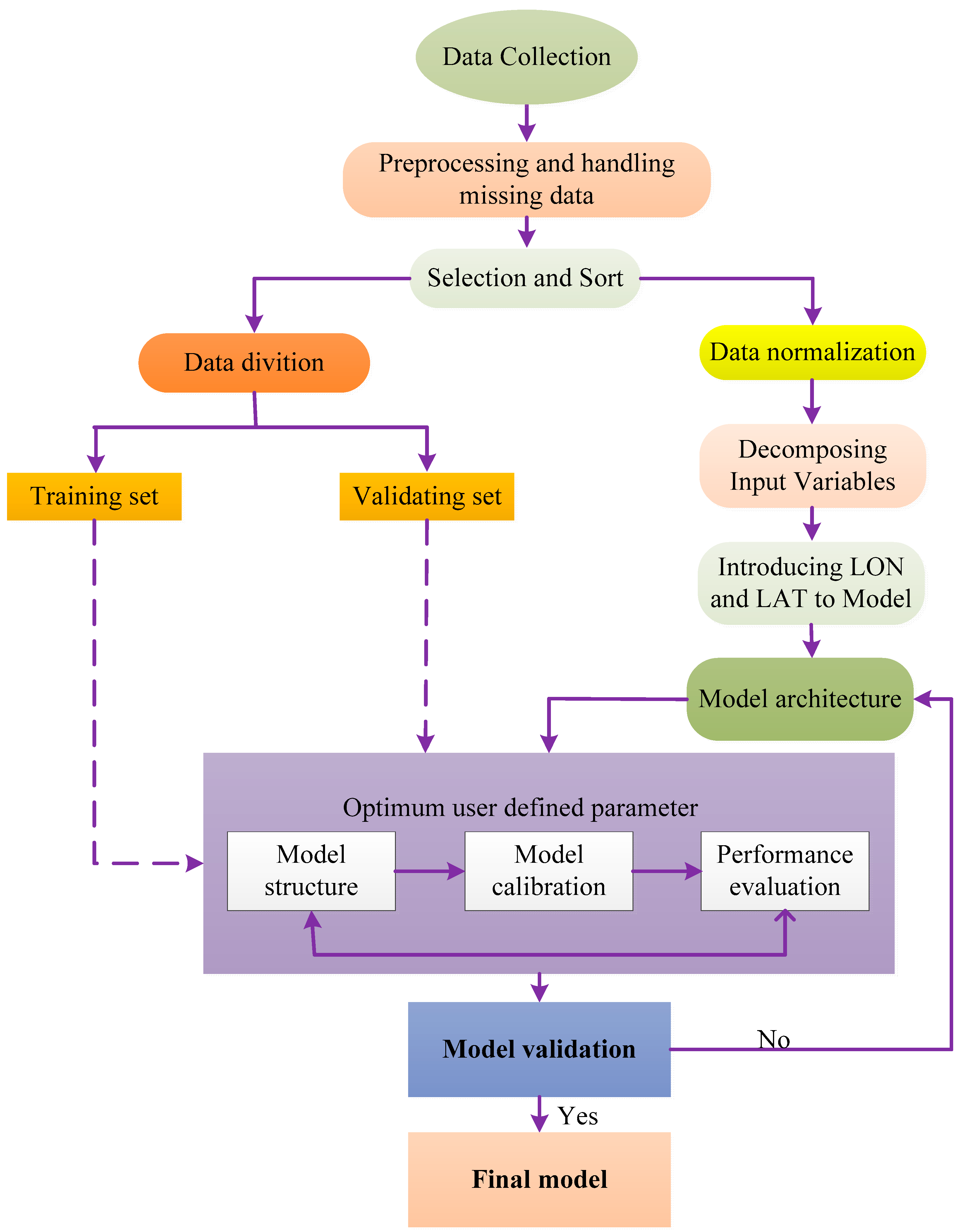
We proposed a CapsNet model that introduced the capsule structure and dynamic routing algorithm to estimate daily PM_2.5 concentrations over China. The longitude (LON) and latitude (LAT) of pixels were used as input parameters to verify whether it is helpful to improve the accuracy of the model. The coefficient of determination (R²), root mean square error (RMSE), mean relative error (MRE), and mean absolute error (MAE) are used as the evaluation metrics.

(2)

To evaluate the CapsNet proposed by us effectively, the DNN model was executed, and the LON and LAT were also included in the DNN model. We discussed the accuracy of CaspNet and DNN in both the cold season and warm season, and the results indicate that CaspNet performs better. Therefore, we used CaspNet to estimate daily PM_2.5 concentrations and analyzed the characteristics of PM_2.5 concentration variations.

(3)

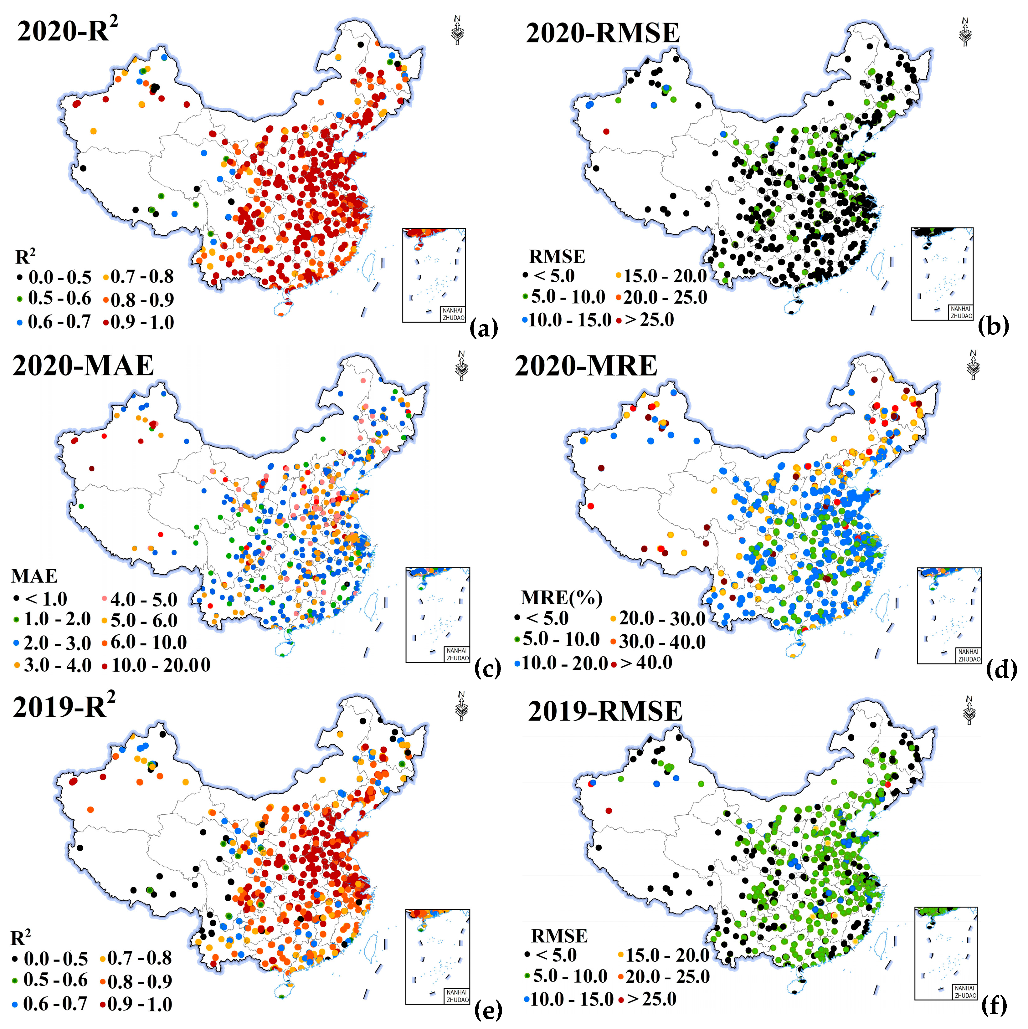
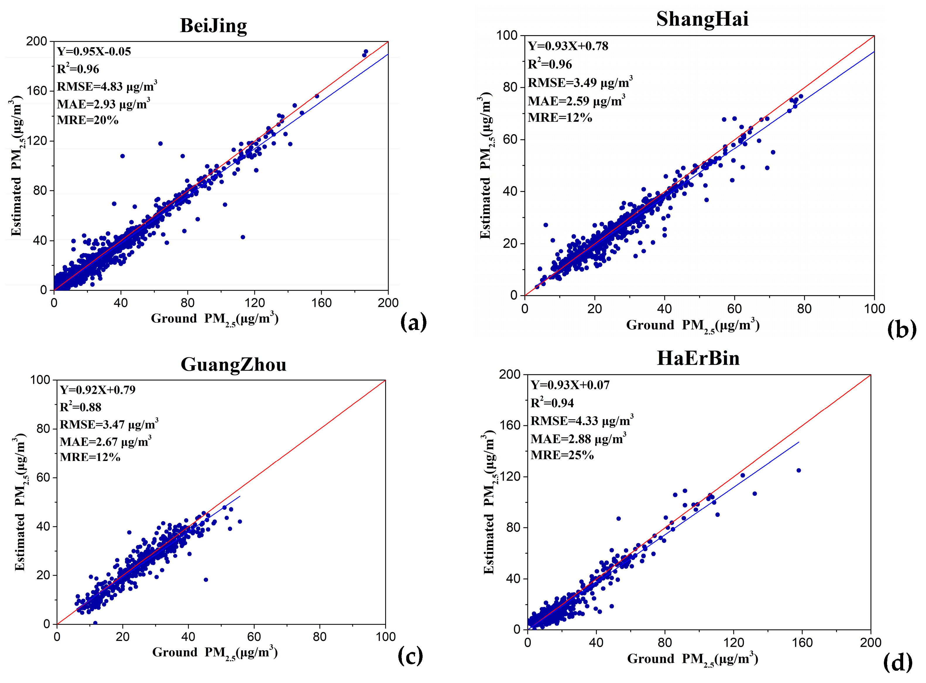
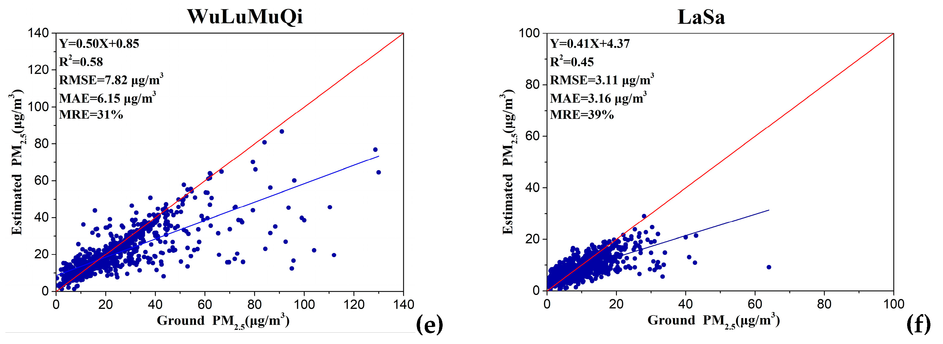
We examined the different advanced capsule layers in CaspNet, which influence the accuracy of PM_2.5 estimation. Multiple capsules and a single weight are better when considering the accuracy and operating efficiency. Moreover, we verified the accuracy of the CaspNet model in different regions.

The flowchart of CapsNet modeling for remote sensing estimation of PM_2.5 concentration is shown in Figure 1 in this study. First, we downloaded ground-measured PM_2.5, satellite data, and meteorological data. All data were preprocessed to obtain a spatialtemporally dataset, and we handed some missing data. Subsequently, the parameters of the input model are discussed, and the CapsNet model could be trained. Finally, evaluation metrics were used to verify the accuracy of PM_2.5 estimation, and then daily PM_2.5 concentrations were obtained. The rest of this paper is structured as follows: Section 2 mainly introduces the CapsNet model; the data used in this study and preprocessing are presented in Section 3; the experimental results are analyzed in Section 4; Section 5 discusses the advantage and disadvantage of this model; and the final section briefly concludes our work.

2. Methodology

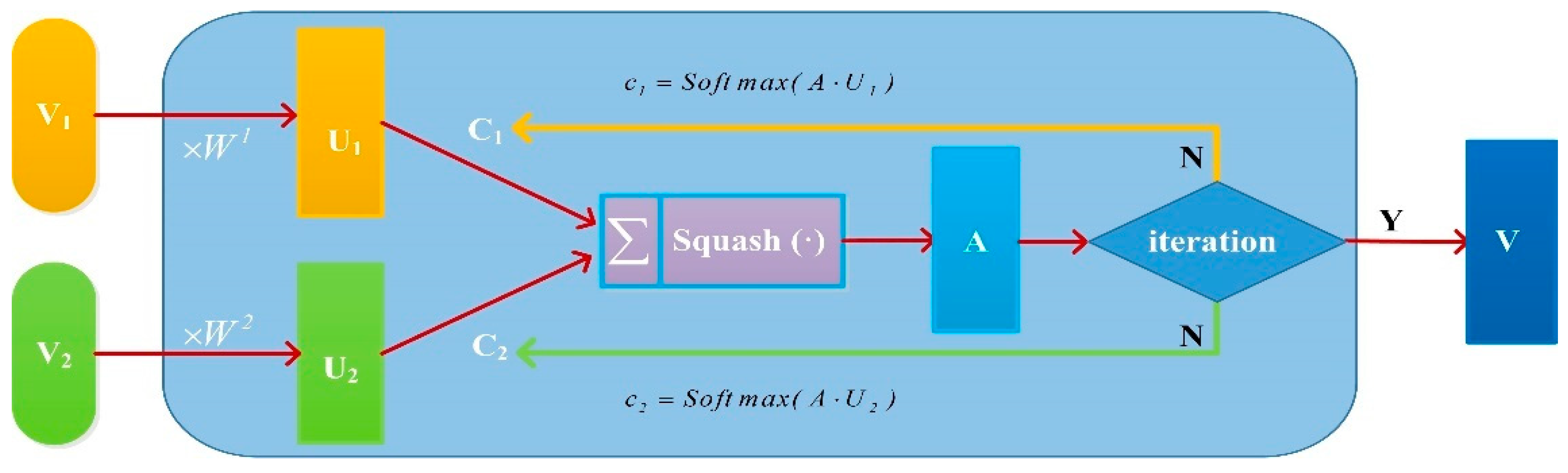
2.1. CapsNet Structure

A CapsNet model, which integrates multiple-source satellite products (e.g., aerosol optical depth and NDVI) and ground-based PM_2.5 measurements, meteorological parameters, and day of year (DOY), is proposed to estimate PM_2.5 concentration.

As shown in Figure 2, the structure of CapsNet consists of three parts: fully connected layer (FC), capsule neuron structure, and dynamic routing algorithm [32]. The first part is the fully connected layer (FC) in the convolutional neural network, where it is used for the initial feature extraction of the input factors. The second part is the primary capsule layer, which captures the features of the data and generates combinations. Subsequently, the capsule carrier is fed into the digitCaps layer. A dynamic routing algorithm (the third part) is used between the primary capsule layer and the digitCaps layer to iteratively update the weights, and it enables the digitCaps layer to extract entity features from low-level capsules and capture geometric relationships. Finally, to achieve the estimation results, the generated vector neurons were filtered, and the capsule with the highest probability was chosen. Especially, to balance the relationship between model complexity and training accuracy, we found through repeated experiments that the training accuracy exceeds the existing model when the number of nodes in the fully-connected layer of the network was set to 200, the primary capsule layer was 64 × 8 × 1, and the shape of the digitCaps layer was 4 × 16 × 1. Therefore, we designed a capsule network model for PM_2.5 concentration estimation based on the idea of the dynamic routing algorithm.

2.2. The Dynamic Routing Algorithm

The logical structure of the dynamic routing algorithm is shown in Figure 3. The neurons in the capsule layer are composed of a set of vectors. The information transmission of neurons is completed by calculating the similarity between the capsules. The information received by capsules of different levels is determined by the routing coefficients. Therefore, a dynamic routing algorithm is used between the primary capsule layer and the digitCaps layer to iteratively update the routing coefficients, and the routing coefficients probability have the following properties: (1) the values for each dimension are non-negative; (2) the sum of all dimensions is equal to 1; (3) the length of weight probability is equal to the number of capsules in the next layer; and (4) the weight probability is determined by updating the dynamic routing algorithm. The details of the dynamic routing algorithm are as follows.

Given the capsule vector ${\mathrm{V}}_1$ and ${\mathrm{V}}_2$, the prediction vector ${\mathrm{U}}_1$ and ${\mathrm{U}}_2$ are calculated by ${\mathrm{U}}_1={\mathrm{V}}_1{\ast \mathrm{W}}^1$ and ${\mathrm{U}}_2={\mathrm{V}}_2{\ast \mathrm{W}}^2$, respectively, where ${\mathrm{W}}^1$ and ${\mathrm{W}}^2$ are the weight matrix trained by the gradient descent algorithm. After taking into account routing coefficients ${\mathrm{C}}_1$ and ${\mathrm{C}}_2$, and a nonlinear normalization function squash, the capsule vector is calculated by $\mathrm{A}=\mathrm{Squshing}\left({\mathrm{C}}_1{\ast \mathrm{U}}_1+{\mathrm{C}}_2{\ast \mathrm{U}}_2\right)$. The multiple iterations algorithm was executed by dynamically updating the routing coefficients ${\mathrm{C}}_1$ and ${\mathrm{C}}_2$ with the geometric agreement. Here, ${\mathrm{C}}_1$ and ${\mathrm{C}}_2$ reflect the probability that the lower-level capsule is assigned to the higher-level one. After a few iterations (the number of iterations is set as 3 in this study), lower-level capsules with strong agreements will dominate the contribution to the A capsule. The result can be deduced from the norm of the output capsule vector. By virtue of this algorithm, CapsNets can not only extract information from lower-level capsules, but also preserve their geometric relationships [32].

2.3. Parameters Setting

All comparation experiments of parameter settings were run under the same environment, and the main experimental parameters are set as follows: the initial learning rate was set as 10⁻⁴; batch was 4000; epoch was 900; the activation function of the first two fully connected layers was a rectified linear unit (ReLU); the activation function of the capsule layer was Squash with novel nonlinear activation functions for vectors; the last layer was the output layer without the activation function; the optimizer of the model was selected as Adam, which was used with ${\beta }_1=0.9$ and ${\beta }_2=0.999$ as weight decay; and the loss function was the mean square error (MSE). This study finally employed a total of 11 feature parameters, namely, LON, LAT, AOD, RH, VWS, HWS, BLH, SP, TP, NDVI, and DOY. Various feature data often have different dimensions, resulting in a large numerical gap between different feature data. Following data screening and sorting, the dataset was randomly divided into a training dataset and a validation dataset at a ratio of 8:2.

2.4. Evaluation Metric

To complete the quantitative evaluation of the capability of the constructed CapsNet model, this study selected R², RMSE, MRE, and MAE as the evaluation metrics. R², RMSE, MRE, and MAE can be represented as follows:

$${\mathrm{R}}^2=1-\frac{{{\displaystyle \sum }}_{i=1}^n{\left(\widehat{y_i}-y_i\right)}^2}{{{\displaystyle \sum }}_{i=1}^n{\left(\overline{y_i}-y_i\right)}^2}$$

(1)

$$\mathrm{RMSE}=\sqrt{\frac{1}{n}{\displaystyle \sum }_{i=1}^n{\left(\widehat{y_i}-y_i\right)}^2}$$

(2)

$$\mathrm{MRE}=\frac{100\%}{n}{\displaystyle \sum }_{i=1}^n\frac{\left|y_i-\widehat{y_i}\right|}{y_i}$$

(3)

$$\mathrm{MAE}=\frac{1}{\mathrm{n}}{\displaystyle \sum }_{i=1}^n\left|y_i-\widehat{y_i}\right|$$

(4)

where $\overline{y_i}$, $\widehat{y_i}$, and $y_i$ are the mean, estimation, and ground-measured PM_2.5 concentration, respectively. n is the total dataset.

3. Data and Preprocessing

3.1. The Ground-Based PM_2.5

Ground-based PM_2.5 data were downloaded from the China Environmental Monitoring Center, providing hourly PM_2.5 ground-based monitoring data (http://106.37.208.233:20035/). In this study, we obtained data from 2018 to 2020, and the distribution of the sites is displayed in Figure 4. The station network is unevenly distributed, with dense stations located in eastern China and sparse stations in western China. To ensure the reliability of the monitoring, those days that had no more than 18 h of valid measurements were deleted from the datasets.

3.2. AOD Products

We used the 1 km MODIS/Aqua AOD products inverted by the Multi-Angle Implementation of Atmospheric Correction algorithm (MAIAC). The overpass time of satellite is about 13:30 (Beijing Time), so the results in this study only reflect PM_2.5 concentration in this time of day. Compared with the commonly used MODIS dark target and deep blue algorithm products (3 km/10 km), MAIAC AOD has a better spatial resolution (1 km), making it ideal for sensitively representing the continuous spatial change of air pollutants and pinpointing PM_2.5 hotspot sources [37,38,39]. The MAIAC has a similar accuracy to the dark target algorithm under the vegetation surface, but it is better than the deep blue algorithm under the bright surface [40]. In addition, the cloud masking method of the MAIAC algorithm based on time series observations can strictly remove clouds, melting snow and ice areas, making the product suitable for monitoring [41]. The AOD products can be downloaded from the National Aeronautics and Space Administration (NASA) (https://ladsweb.modaps.eosdis.nasa.gov/).

3.3. European Centre for Medium-Range Weather Forecasts Data and Other Auxiliary Data

The European Centre for Medium-Range Weather Forecasts (ECMWF) re-analysis (ERA) is a widely used meteorological reanalysis dataset with benefits such as continuous series and regional coverage. According to the literature, the ERA data in the lower and middle troposphere are closer to sounding data than other reanalysis products [42]. With a temporal resolution of one hour and a spatial resolution of 0.25°, ERA5 was officially released in 2017, and the meteorological parameters primarily include relative humidity (RH, unit: %), vertical and horizontal wind speed (VWS/HWS, unit: m/s), boundary layer height (BLH, unit: m), surface pressure (SP, unit: Pa), and surface temperature (TP, unit: K). To enhance the spatial and temporal sensitivity of the model, this study introduced the longitude (LON) and latitude (LAT) coordinates of the image element. In addition, the normalized difference vegetation index (NDVI) from the MODIS satellite was downloaded, namely MOD13 products, which have a spatial resolution of 1 km.

3.4. Data Preprocessing

To ensure the spatial and temporal consistency of all data, all data were reprocessed to generate a full dataset acceptable for this study. To maintain the consistency of spatial resolution, reprojection was conducted on all data to the WGS84 geographic coordinate system. Because the NDVI, AOD, and meteorological parameters have different spatial resolutions, the meteorological and NDVI data were resampled to 1 × 1 km using the bilinear interpolation method. The corresponding pixel values (satellite and meteorological data) were extracted with the longitude and latitude information of PM_2.5 monitoring stations to produce the corresponding records. To be as consistent in temporal as possible, the average PM_2.5 concentration of ground-based monitoring was determined half an hour before and after the satellite pass time to maintain the consistency between ground-based and satellite observations, because the scanning time of Aqua/AOD data was approximately 13:30 daily.

4. Experiment Analysis

4.1. Experimental Results

4.1.1. Normalization Methods

In the process of model training, a large number of dimensional values greatly weaken the role of small dimensional values in the model, preventing the model from being correctly trained to obtain accurate fitting relationships. To eliminate the effects of dimensional differences, all data need to be normalized. The results of different normalization methods can ultimately affect the results of the model. In the mainstream normalization methods, we separately discussed the minimum–maximum method and standard score (Z-Score) method, and the methods can be expressed as follows:

$$\mathrm{minimum}-\mathrm{maximum}:I=\frac{I-I_{\mathit{min}}}{I_{\mathit{max}}-I_{\mathit{min}}}$$

(5)

$$\mathrm{Z}-\mathrm{Score}:I=\frac{I-I_{\mathit{mean}}}{I_{\mathit{std}}}$$

(6)

where I is the feature data and $I_{min}$, $I_{max}$, $I_{mean}$, and $I_{std}$ denote the minimum, maximum, mean value, and standard deviation in the feature data, respectively.

The above two methods were used to conduct normalization experiments on the same dataset, and we calculated normalization rules on the data of the training set and applied them to the validation set for experiments. The experimental results are shown in

Table 1. Experimental results of two normalization methods.

Methods	Dataset	R2	RMSE	MRE	MAE
minimum–maximum	Train	0.89	9.84	30%	6.06
	Validation	0.79	13.30	40%	8.06
Z-score	Train	0.96	6.39	18%	3.23
	Validation	0.81	12.75	41%	7.93

. According to the results of the normalization methods, R², RMSE, MRE, and MAE are 0.81, 12.75 μg/m³, 41%, and 7.93 μg/m³, respectively, in validation datasets by the Z-score, which is beyond that of the minimum–maximum method; therefore, the next experimental datasets were normalized by the Z-Score.

4.1.2. Parameter Validation

Other research has examined meteorological parameters, NDVI, and DOY as input parameters impacting PM_2.5 [30], while we mainly focused on the effect of LON and LAT information on the accuracy of model fitting.

Table 2. Comparison validation of the CapsNet model fitting accuracy with and without longitude and latitude (2018–2020).

Year	Factors	Train (Validation)
		R2	RMSE	MRE	MAE
2018	-	0.92 (0.75)	9.92 (16.60)	26% (45%)	4.84 (10.01)
	LON, LAT	0.94 (0.82)	7.99 (13.30)	21% (35%)	4.58 (8.66)
2019	-	0.90 (0.78)	8.96 (13.46)	18% (44%)	3.55 (8.58)
	LON, LAT	0.91 (0.83)	8.45 (11.03)	24% (36%)	5.11 (7.21)
2020	-	0.92 (0.80)	8.75 (12.31)	24% (42%)	4.77 (8.11)
	LON, LAT	0.94 (0.84)	5.34 (10.98)	24% (37%)	3.25 (6.59)

shows the effect of including LON and LAT information factors in the training data on the simulation outcomes. The training and validation results of the CapsNet model for 2018, 2019, and 2020 data showed R² value increasing by 0.05, 0.05, and 0.04; RMSE decreasing by 3.30 μg/m³, 2.43 μg/m³, and 1.33 μg/m³; MRE decreasing by 10%; and MAE decreasing by 1.35 μg/m³, 1.37 μg/m³, and 1.57 μg/m³. Therefore, the introduction of LON and LAT pixel information as input parameters in this study performed better on both training and validation datasets. The density scatter plots of the fitting results are shown in Figure 5. There were differences in model accuracy from 2018 to 2020. The majority of the data are concentrated around the 1:1 fit line, the slope of the fit line is greater than 0.8, and the difference in the coefficient of determination of the validation set is small, which indicates that CapsNet obtained good accuracy.

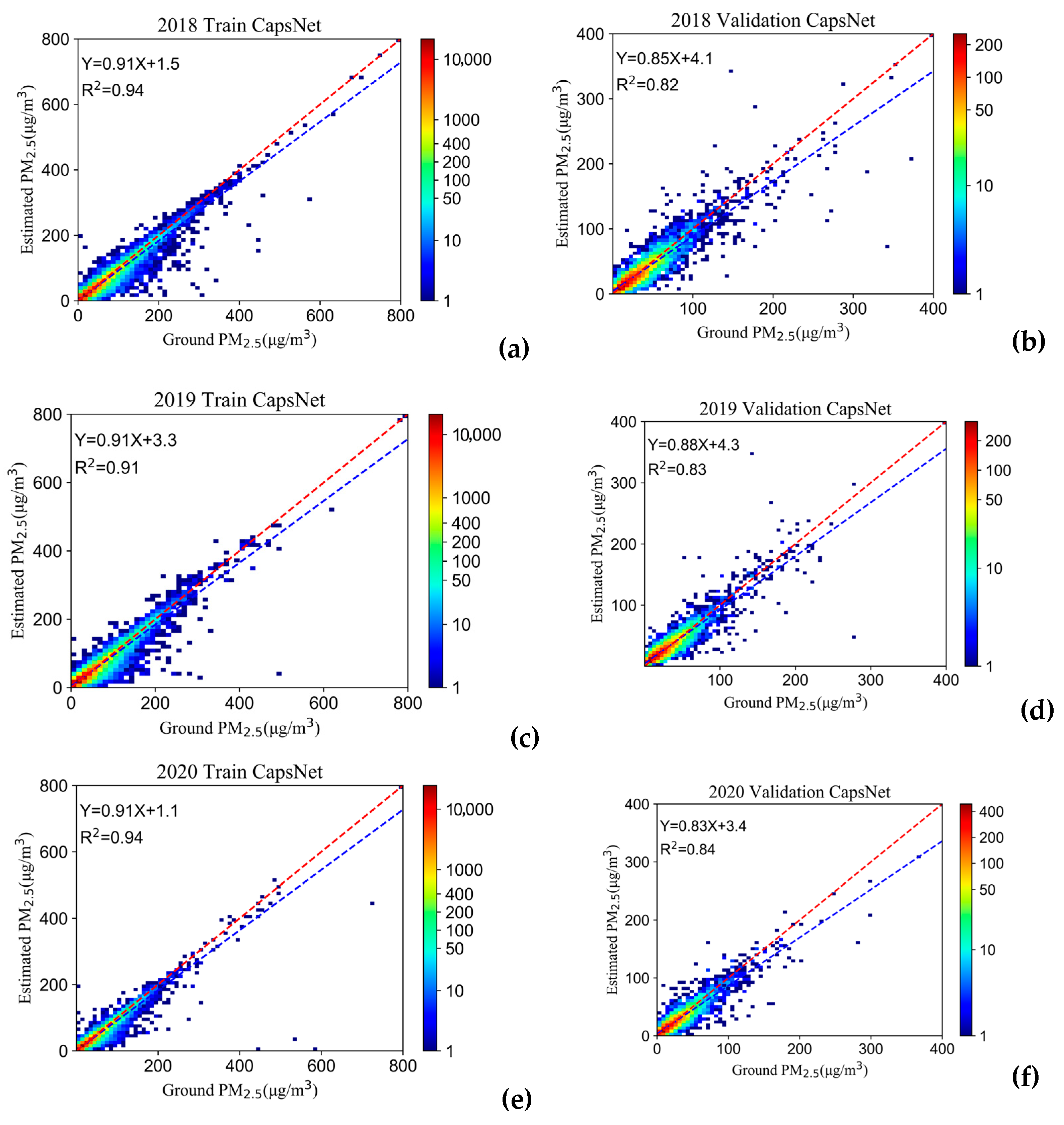
4.1.3. Accuracy Validation

Training and validation of the data samples collated in this study area revealed that different regions may lead to differences in the fitting accuracy of each station. R², RMSE, MRE, and MAE of the fitted sites are plotted in Figure 6, which shows that the parameters have significant consistency in spatial distribution. In 2020, for example, most stations in the Liaoning, Beijing, Tianjin, Hebei, Shandong, Shanxi, Henan, Hubei, Anhui, Shanghai, and Hunan regions had R² values greater than 0.9, with high fitting accuracy. The R² values for most stations in the Jilin, Zhejiang, Fujian, Jiangxi, Guangdong, Guangxi, Shanxi, Yunnan, Guizhou, Sichuan Basin, and Chongqing areas were between 0.8 and 0.9, with R² values greater than 0.9 for a few stations and R² values between 0.5 and 0.7 for a few others. The R² values for the Tibet, Xinjiang, Qinghai, Inner Mongolia, and Heilongjiang regions are all lower. The RMSEs of most stations were less than 5 μg/m³, with relatively high values between 5 and 10 μg/m³ in Beijing, Tianjin, Hebei, Shandong, Henan, and other regions, while the RMSEs of sites in Xinjiang were between 10 and 15 μg/m³, with only one site larger than 15 μg/m³. MAEs were less than 5 μg/m³ in 93% of the locations. The MREs were mainly between 10 and 20%, while the MREs were mainly distributed between 20 and 30% in Tibet and Heilongjiang.

4.2. Model Comparison

We used the DNN model to estimate the PM_2.5 concentration to compare the ability of the CapsNet model. We selected four hidden layers with the structure of 300-300-10-20; please refer to the study by Sun [16] for other detailed parameters. The same dataset as the CapsNet model was used for DNN.

Table 3. Comparison validation of the DNN model fitting accuracy with and without longitude and latitude (2018–2020).

Year	Factors	Train (Validation)
		R2	RMSE	MRE	MAE
2018	-	0.92 (0.74)	9.43 (17.10)	25% (47%)	5.06 (10.36)
	LON, LAT	0.94 (0.79)	7.89 (15.14)	22% (40%)	4.52 (9.14)
2019	-	0.90 (0.77)	8.96 (13.83)	18% (42%)	3.55 (8.65)
	LON, LAT	0.94 (0.81)	7.14 (12.43)	21% (37%)	3.87 (7.83)
2020	-	0.94 (0.73)	5.57 (13.27)	23% (45%)	3.46 (7.90)
	LON, LAT	0.94 (0.78)	5.63 (12.00)	29% (42%)	3.64 (7.07)

shows the results of building the DNN model using the same dataset to assess the ability of the CapsNet model. The results of using LON and LAT as input parameters in the DNN model were more accurate, especially in the validation dataset, similar to the findings of the CapsNet model. When comparing the DNN and CapsNet models, we found that the R² values improved by 3%, 2%, and 6% from 2018 to 2020, respectively, when using the CapsNet model. The RMSEs decreased by 1.84, 1.40, and 1.02 μg/m³, respectively, in different years. The MREs and MAEs showed some reduction.

To assess the fitting capacity of the two models in terms of seasons, the data were divided into the cold season (January, February, and September–December) and warm season (March–August), as shown in

Table 4. The DNN and CapsNet model fitting accuracies in both the cold and warm seasons in 2018, 2019, and 2020.

Time	Method	Train or Validation	R2	RMSE	MRE	MAE
2018cold	DNN	Train	0.95	6.65	18%	3.67
		Validation	0.83	14.16	39%	8.76
	CapsNet	Train	0.95	7.09	18%	3.75
		Validation	0.83	13.93	36%	8.46
2018warm	DNN	Train	0.94	8.47	18%	4.27
		Validation	0.72	19.39	38%	10.17
	CapsNet	Train	0.95	6.29	15%	2.73
		Validation	0.75	18.23	37%	9.82
2019cold	DNN	Train	0.95	7.44	17%	3.68
		Validation	0.82	13.33	36%	8.40
	CapsNet	Train	0.93	8.86	23%	4.67
		Validation	0.84	12.52	36%	7.87
2019warm	DNN	Train	0.94	6.22	22%	3.19
		Validation	0.75	12.59	47%	7.47
	CapsNet	Train	0.88	8.63	26%	4.52
		Validation	0.77	12.20	42%	7.03
2020cold	DNN	Train	0.95	6.18	19%	2.98
		Validation	0.81	11.52	33%	7.36
	CapsNet	Train	0.95	6.29	15%	2.73
		Validation	0.82	11.50	31%	7.34
2020warm	DNN	Train	0.94	5.13	19%	2.53
		Validation	0.67	11.15	43%	6.76
	CapsNet	Train	0.94	5.25	14%	2.35
		Validation	0.72	10.14	43%	6.64

. Both the CapsNet and DNN models exhibited higher accuracy in the cold season than in the warm season, and the R² values were 0.83 ± 0.02 and 0.74 ± 0.03 in the validation dataset, respectively. The RMSEs, MAEs, and MREs also had large differences. When comparing the CapsNet and DNN models on the training dataset in the cold and warm seasons, the difference in R² values was approximately 0.2, and the DNN models showed better performance. However, we found that the CapsNet model was better in the validation dataset, and then the DNN model showed severe overfitting. For example, R², RMSE, MRE, and MAE of the CapsNet model the warm 2020 validation dataset were 0.72, 10.14 μg/m³, 43%, and 6.64 μg/m³, respectively, but they were 0.67, 11.15 μg/m³, 43%, and 6.76 μg/m³, respectively, in the DNN model. Overall, the CapsNet model had a higher fitting accuracy.

4.3. Spatiotemporal Patterns of PM_2.5

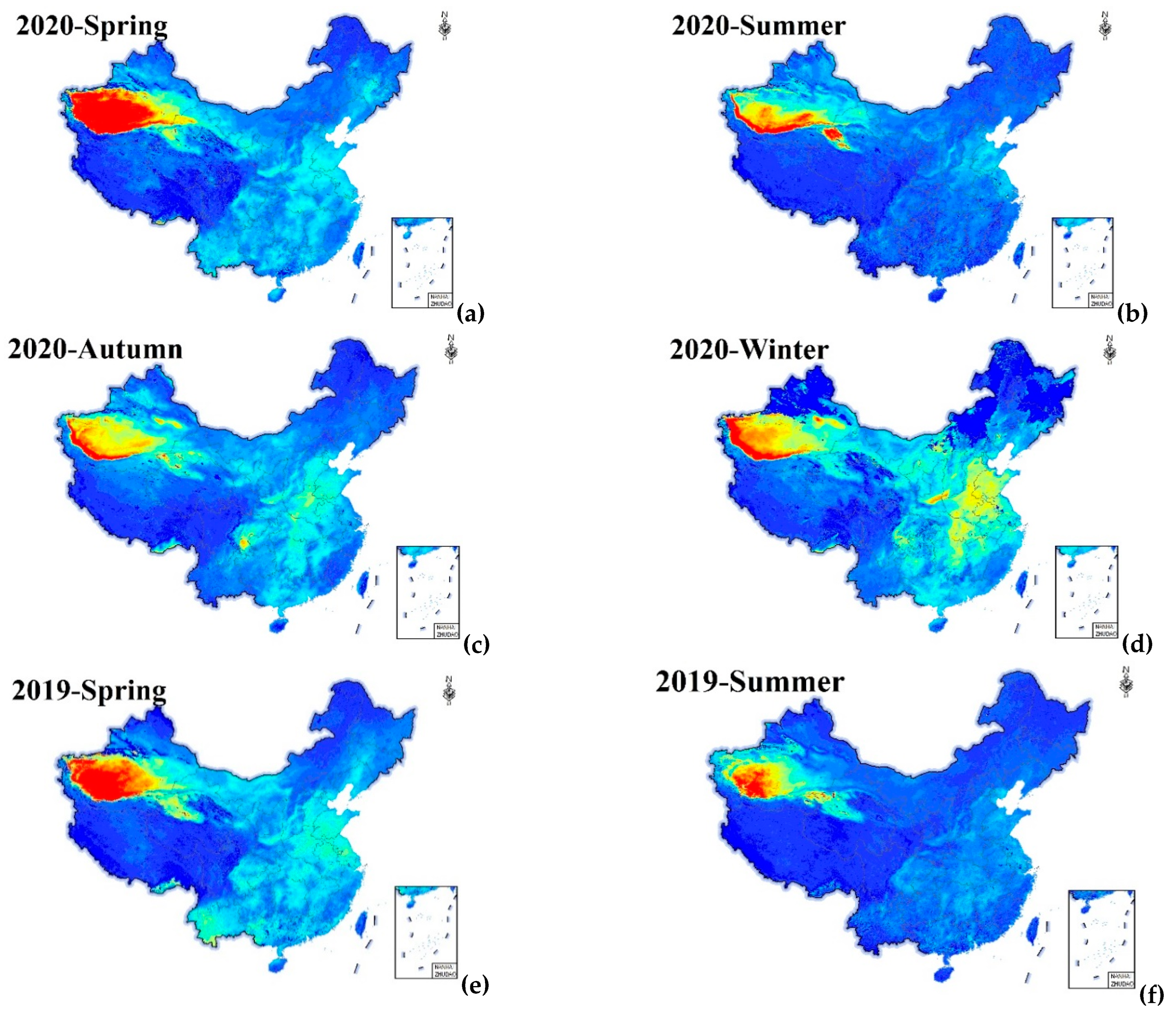
4.3.1. Seasonal Distribution

According to the comparative experiments in Section 4.2, the CapsNet model had better accuracy, and we used it to estimate daily PM_2.5 concentrations from 2018 to 2020. The spatial distribution of the seasonal average PM_2.5 concentration is shown in Figure 7. Comparing four seasons, we found that the PM_2.5 concentration in winter (December, January, and February) > spring (March, April, and May) > autumn (September, October, and November) > summer (June, July, and August) in 2018 and 2019, and the phenomenon was similar to other studies. However, in 2020, the PM_2.5 concentration in autumn exceeded that in spring, which can be explained by the fact that the industrial and anthropogenic activities were limited in spring owing to the COVID-19 epidemic, and the emissions of pollutants into the atmosphere were reduced. With the containment of the COVID-19 epidemic, the economy has begun to recover by increasing industrial and human activity; therefore, the PM_2.5 concentration could increase. For example, Song et al. discussed the air pollution during COVID-19 lockdown and found the PM_2.5 decreased by 44.1% in February 2020. Liu et al. demonstrated that the COVID-19 lockdown led to the lowest intensity of human activities in recent decades, which provided a unique opportunity to gain insights into the relationship between emission sources and aerosol chemistry [43]. The COVID-19 lockdown led to significant decreases in PM_2.5. Therefore, the trends of PM_2.5 concentration are consistent with previous studies [44]. We can see that the PM_2.5 concentration in summer was the lowest, which was mainly influenced by atmospheric conditions. Comparing the winter and spring from 2018 to 2020, we found an obvious gradual reduction in the PM_2.5 concentration, especially in the Beijing–Tianjin–Hebei and southwestern regions.

4.3.2. Annual Distribution

The annual average PM_2.5 concentration over China was calculated and is shown in Figure 8. According to Figure 8, the PM_2.5 concentrations estimated by satellite and ground-based monitoring were highly consistent in spatial distribution, when remote sensing data were available. The heavily polluted areas were primarily in the Taklimakan Desert, North China Plain, and Sichuan Basin in mid-China. In addition, PM_2.5 concentrations in 2018–2020 show a decreasing trend, which was related to a series of emission reduction measures taken by the environmental regulatory authorities, while a greater reduction in PM_2.5 concentrations in 2020 may have been related to the reduction of industrial activities and anthropogenic emissions during the COVID-19 epidemic.

5. Discussion

The different advanced capsule layers influenced the fitting accuracy of the results, and we discussed three different structures: (1) an advanced capsule layer of a single capsule, that is, all the information of the primary capsule layer was collected into one capsule for output; (2) an advanced capsule layer with multiple capsules and a single weight, in which we set four capsule layers; and (3) multi-capsule and multi-weight, thus setting a weight for each advanced capsule instead of using shared weights. Taking the 2019 as an example, the results are shown in

Table 5. The results of different capsule structures.

Structures	R2	RMSE	MRE	MAE
single capsule	0.92	8.79	0.37	5.87
Multiple capsules and single weight	0.93	8.02	0.22	4.14
Multi-capsule and multi-weight	0.93	7.85	0.28	4.98

. Among the three structure designs, the single-capsule structure achieved the worst fitting accuracy. Because all information was input to one high-level capsule, it could not reflect the screening characteristics of the information, and the accuracy was degraded to the fully connected structure. Multi-capsule and single-weight and multi-capsule and multi-weight methods have achieved similar R² values. The multi-weight effect obtained a lower RMSE, but the single weight was better in MRE and MAE. In addition, the multi-capsule and multi-weight structure spent more time in the training stage. Therefore, considering the accuracy and running efficiency, the multi-capsule and single weight used in this study was a better choice.

In addition, we selected PM_2.5 monitoring stations in typical regions for fitting assessment, and selected station datasets on a city basis (with 2020 data as an example). Beijing on the North China Plain and Shanghai on the middle and lower Yangtze River Plain were selected, both of which are located in areas with high PM_2.5 concentrations and have dense ground-based stations around the cities. Afterward, Lhasa in Tibet Province and Urumqi in Xinjiang Province were selected, which are located in south-central Tibet and northern Xinjiang, respectively, and have few ground-based stations around them. Guangzhou, which has experienced large climate change in southern China, and Harbin, which has a stable climate, were also selected, and the validation scatter plot is shown in Figure 9. The results showed that the accuracy is highest in Beijing and Shanghai, followed by Harbin and Guangzhou, and the lowest in Urumqi and Lhasa, indicating that the accuracy of the model may be related to the number of stations, regional distribution, and weather conditions. In addition, the accuracy of AOD retrieval shows a significant difference in different regions. For example, there was a complex aerosol type (mainly dust) in Xinjiang province, and the accuracy is relatively low. In the northeast, there was a large amount of snow and ice cover, leading to ineffective retrieval AOD in winter.

Finally, this study applied the CapsNet model to the field of PM_2.5 estimation for the first time and introduced longitude and latitude information to reflect the spatial variation, resulting in improved findings, but there are still some limitations. (1) Because the MAIAC AOD lacked data under clouds, the estimation results only represented the PM_2.5 concentration when data were available. In the case of clouds, ground-based observation data are combined to obtain the annual average (365 days) results of air quality conditions under clouds. (2) According to the Table 3, the accuracy of the CapsNet model was different in 2018, 2019, and 2020, which may be affected by dataset quality. Besides, there were significant differences between the seasons according to the results of the models constructed in Table 4, and the specific influencing factors need to be investigated further. (3) This study mainly considered the feasibility of the CapsNet model for estimating PM_2.5 concentrations, and only obtained meteorological parameters and the NDVI to construct the model for comparison with the DNN. More factors affecting PM_2.5 generation can be considered in future work.

6. Conclusions

In this study, we proposed a CapsNet model to estimate the daily PM_2.5 concentrations at a national scale from 2018 to 2020. The CapsNet model was applied to atmospheric research for the first time. First, we discussed whether introducing longitude and latitude information as input factors could improve the accuracy of both the CapsNet and DNN models. Compared with the DNN models with the same input parameters, the CapsNet model developed by us achieved the better validation performance. Next, we separately built CapsNet and DNN in the cold and warm seasons. The results indicated that the cold season had better fitting accuracy. The PM_2.5 seasonal and annual distributions were shown in 2018–2020, which presented that the PM_2.5 concentration decreased. We found that the PM_2.5 concentration in autumn was beyond that in spring of 2020, which could have mainly been influenced by the COVID-19 epidemic. In addition, we found that there were some regional disparities in model accuracy, and the overall accuracy is higher. Not only can the CapsNet model suggested in this work be used to predict PM_2.5 concentrations, but it can also be used to estimate other atmospheric components.

References

1. Crouse, D.L.; Peters, P.A.; Donkelaar, A.V.; Goldberg, M.S.; Villeneuve, P.J.; Brion, O.; Khan, S.; Atari, D.O.; Jerrett, M.; Pope, C.A.; et al. Risk of Nonaccidental and Cardiovascular Mortality in Relation to Long-term Exposure to Low Concentrations of Fine Particulate Matter: A Canadian National-Level Cohort Study. Environ. Health Perspect. 2012, 120, 708–714. [Google Scholar] [CrossRef] [PubMed]
2. Chen, J.P.; Yin, J.H.; Zang, L.; Zhao, M.D. Stacking machine learning model for estimating hourly PM2.5 in China based on Himawari 8 aerosol optical depth data. Sci. Total Environ. 2019, 697, 134021. [Google Scholar] [CrossRef]
3. Wei, J.; Huang, W.; Li, Z.P.; Xue, Y.P.; Peng, Y.R.; Sun, L.; Cribb, M. Estimating 1-km-resolution PM2.5 concentrations across China using the space-time random forest approach. Remote Sens. Environ. 2019, 231, 111221. [Google Scholar] [CrossRef]
4. Guo, B.; Zhang, D.M.; Pei, L.; Su, Y.; Wang, X.X.; Bian, Y.; Zhang, D.H.; Yao, W.Q.; Zhou, Z.X.; Guo, L.Y. Estimating PM2.5 concentrations via random forest method using satellite, auxiliary, and ground-level station dataset at multiple temporal scales across China in 2017. Sci. Total Environ. 2021, 778, 146228. [Google Scholar] [CrossRef] [PubMed]
5. Liang, X.Y.; Zhang, S.J.; Wu, X.; Guo, X.; Han, L.; Liu, H.; Wu, Y.; Hao, J.M. Air quality and health impacts from using ethanol blended gasoline fuels in China. Atoms. Environ. 2020, 228, 117396. [Google Scholar] [CrossRef]
6. Zhang, T.H.; Zhu, Z.M.; Gong, W.; Zhu, Z.R.; Sun, K.; Wang, L.C.; Huang, L.C.; Mao, X.F.; Shen, H.F.; Li, Z.W.; et al. Estimation of ultrahigh resolution PM2.5 concentrations in urban areas using 160m Gaofen-1 AOD retrievals. Remote Sens. Environ. 2018, 216, 91–104. [Google Scholar] [CrossRef]
7. Hutchison, K.D.; Smith, S.; Faruqui, S.J. Correlating MODIS aerosol optical thickness data with ground-based PM2.5 observations across Texas for use in a real-time air quality prediction system. Atoms. Environ. 2005, 39, 7190–7203. [Google Scholar] [CrossRef]
8. Yao, F.; Si, M.; Li, W.; Wu, J. A multidimensional comparison between MODIS and VIIRS AOD in estimating ground-level PM2.5 concentrations over a heavily polluted region in China. Sci. Total Environ. 2018, 618, 819–828. [Google Scholar] [CrossRef]
9. Sreekanth, V.; Mahesh, B.; Niranjan, K. Satellite Remote Sensing of Fine Particulate air pollutants over Indian Mega Cities. Adv. Space Res. 2017, 60, 2268–2276. [Google Scholar] [CrossRef]
10. Ma, Z.; Hu, X.; Sayer, A.M.; Levy, R.; Zhang, Q.; Xue, Y.; Tong, S.; Bi, J.; Huang, L.; Liu, Y. Satellite-Based Spatiotemporal Trends in PM2.5 Concentrations: China, 2004–2013. Environ. Health Perspect. 2016, 124, 184–192. [Google Scholar] [CrossRef] [Green Version]
11. Zhang, Y.; Li, Z. Remote sensing of atmospheric fine particulate matter (PM2.5) mass concentration near the ground from satellite observation. Remote Sens. Environ. 2015, 160, 252–262. [Google Scholar] [CrossRef]
12. Lee, H.J.; Liu, Y.; Coull, B.A.; Schwartz, J.; Koutrakis, P. A novel calibration approach of MODIS AOD data to predict PM2.5 concentrations. Atmos. Chem. Phys. 2011, 11, 9769–9795. [Google Scholar] [CrossRef] [Green Version]
13. You, W.; Zang, Z.; Pan, X.; Zhang, L.; Chen, D. Estimating PM2.5 in Xi’an, China using aerosol optical depth: A comparison between the MODIS and MISR retrieval models. Sci. Total Environ. 2015, 505, 1156–1165. [Google Scholar] [CrossRef] [PubMed]
14. Liu, Y.; Franklin, M.; Kahn, R.; Koutrakis, P. Using aerosol optical thickness to predict ground-level PM2.5 concentrations in the St. Louis area: A comparison between MISR and MODIS. Remote Sens. Environ. 2007, 107, 33–44. [Google Scholar] [CrossRef]
15. Liu, Y.; Paciorek, C.J.; Koutrakis, P. Estimating regional spatial and temporal variability of PM2.5 concentrations using satellite data, meteorology, and land use information. Environ. Health Perspect. 2009, 117, 886. [Google Scholar] [CrossRef] [Green Version]
16. Zhang, X.; Hu, H. Improving Satellite-Driven PM2.5 Models with VIIRS Nighttime Light Data in the Beijing–Tianjin–Hebei Region, China. Remote Sens. 2017, 9, 908. [Google Scholar] [CrossRef] [Green Version]
17. Wang, J.; Aegerter, C.; Xu, X.; Szykman, J.J. Potential application of VIIRS Day/Night Band for monitoring nighttime surface PM2.5 air quality from space. Atmos. Environ. 2016, 124, 55–63. [Google Scholar] [CrossRef] [Green Version]
18. Wang, W.; Mao, F.; Du, L.; Pan, Z.; Gong, W.; Fang, S. Deriving Hourly PM2.5 Concentrations from Himawari-8 AODs over Beijing–Tianjin–Hebei in China. Remote Sens. 2017, 9, 858. [Google Scholar] [CrossRef] [Green Version]
19. Mao, F.Y.; Hong, J.; Min, Q.L.; Gong, W.; Zang, L.; Yin, J.H. Estimation hourly full-coverage PM2.5 over China base on TOA reflectance data from the Fengyun-4A satellite. Environ. Pollut. 2021, 270, 116119. [Google Scholar] [CrossRef]
20. Liu, Y.; Park, R.J.; Jacob, D.J.; Qinbin Li, Q.B.; Vasu Kilaru, K.; Sarnat, J. Mapping annual mean ground-level PM2.5 concentrations using Multiangle Imaging Spectroradiometer aerosol optical thickness over the contiguous United States. J. Geophys. Res. Atmos. 2004, 109, D22206. [Google Scholar]
21. Donkelaar, A.V.; Martin, R.V.; Park, R.J. Estimating ground-level PM2.5 using aerosol optical depth determined from satellite remote sensing. J. Geophys. Res. Atmos. 2006, 111, 5049–5066. [Google Scholar]
22. Wang, Z.F.; Chen, L.F.; Tao, J.H.; Zhang, Y.; Su, L. Satellite-based estimation of regional particulate matter (PM) in Beijing using vertical-and-RH correcting method. Remote Sens. Environ. 2010, 114, 50–63. [Google Scholar] [CrossRef]
23. Guo, J.P.; Zhang, X.Y.; Che, H.Z.; Gong, S.L.; An, X.Q.; Cao, C.X.; Guang, J.; Zhang, H.; Wang, Y.Q.; Zhang, X.C.; et al. Correlation between concentrations and aerosol optical depth in eastern China. Atmos. Environ. 2009, 43, 5876–5886. [Google Scholar] [CrossRef]
24. Hu, X.; Waller, L.A.; Al-Hamdan, M.Z.; Crosson, W.L.; Estesjr, M.G.; Estes, S.M.; Quattrochi, D.A.; Sarnat, J.A.; Liu, Y. Estimating ground-level PM2.5 concentrations in the southeastern U.S. using geographically weighted regression. Environ. Res. 2013, 121, 1–10. [Google Scholar] [CrossRef] [PubMed]
25. Guo, Y.X.; Tang, Q.H.; Gong, D.Y.; Zhang, Z.Y. Estimating ground-level PM2.5 concentrations in Beijing using a satellite-based geographically and temporally weighted regression model. Remote Sens. Environ. 2017, 198, 140–149. [Google Scholar] [CrossRef]
26. Liu, Y.; Sarnat, J.A.; Kilaru, V.; Jacob, D.J.; Koutrakis, P. Estimating ground-level PM2.5 in the eastern United States using satellite remote sensing. Environ. Sci. Technol. 2005, 39, 3269. [Google Scholar] [CrossRef] [PubMed] [Green Version]
27. Koelemeijer, R.; Homan, C.D.; Matthijsen, J. Comparison of spatial and temporal variations of aerosol optical thickness and particulate matter over Europe. Atoms. Environ. 2006, 40, 5304–5315. [Google Scholar] [CrossRef]
28. Chu, D.A.; Tsai, T.C.; Chen, J.P.; Cheng, S.C.; Jeng, Y.J.; Chiang, W.L.; Lin, N.H. Interpreting aerosol lidar profiles to better estimate surface PM2.5 for columnar AOD measurements. Atoms. Environ. 2013, 79, 172–187. [Google Scholar] [CrossRef]
29. Lin, C.Q.; Li, Y.; Yuan, Z.B.; Lau, A.K.H.; Li, C.C.; Fung, J.C.H. Using satellite remote sensing data to estimate the high-resolution distribution of ground-level PM2.5. Remote Sens. Environ. 2015, 156, 117–128. [Google Scholar] [CrossRef]
30. Sun, Y.B.; Zeng, Q.L.; Geng, B.; Lin, X.W.; Sude, B.; Chenl, L.F. Deep learning architecture for estimating hourly ground-level PM2.5 using satellite remote sensing. IEEE Geosci. Remote Sens. Lett. 2019, 16, 1343–1347. [Google Scholar] [CrossRef]
31. Li, L.F.; Franklin, M.; Girguis, M.; Lurmann, F.; Wu, J.; Pavlovic, N.; Breton, C.; Gilliland, F.; Habre, R. Spatiotemporal Imputation of MAIAC AOD Using Deep Learning with Downscaling. Remote Sens. Environ. 2020, 237, 111584. [Google Scholar] [CrossRef] [PubMed]
32. Shen, H.F.; Li, T.W.; Yuan, Q.Q.; Zhang, L.P. Estimating Regional Ground-Level PM2.5 Directly from Satellite Top-Of-Atmosphere Reflectance Using Deep Belief Networks. J. Geophys. Res. Atmos. 2018, 123, 13875–13886. [Google Scholar] [CrossRef] [Green Version]
33. Hong, D.F.; Gao, L.R.; Yao, J.; Zhang, B.; Plaza, A.; Chanussot, J. Graph Convolutional Networks for Hyperspectral Image Classification. IEEE Trans. Geosci. Remote Sens. 2021, 59, 5966–5978. [Google Scholar] [CrossRef]
34. Hong, D.F.; Gao, L.R.; Yokoya, N.; Yao, J.; Chanussot, J.; Du, Q.; Zhang, B. More Diverse Means Better: Multimodal Deep Learning Meeets Remote-Sensing Imagery Classificaion. IEEE Trans. Geosci. Remote Sens. 2021, 59, 4340–4354. [Google Scholar] [CrossRef]
35. Sabour., S.; Frosst, N.; Hinton, G. Dynamic routing between capsules. In Proceedings of the Neural Information Processing Systems (NIPS Proceeding), Long Beach, CA, USA, 4–9 December 2017; pp. 3856–3866. [Google Scholar]
36. Afshar, P.; Mohammadi, A.; Plataniotis, K.N. Brain tumor type classification via capsule networks. In Proceedings of the 25th IEEE International Conference on Image Processing, Athens, Greece, 7–10 October 2018; pp. 3129–3133. [Google Scholar]
37. Levy, R.C.; Mattoo, S.; Munchak, L.A.; Remer, L.A.; Sayer, A.M.; Patadia, F.; Hsu, N.C. The Collection 6 MODIS aerosol products over land and ocean. Atmos. Meas. Tech. 2013, 6, 2989–3034. [Google Scholar] [CrossRef] [Green Version]
38. Xie, Y.Y.; Wang, Y.X.; Zhang, K.; Dong, W.H.; Lv, B.; Bai, Y.Q. Daily estimation of ground-level PM2.5 concentrations over Beijing using 3 km resolution MODIS AOD. Environ. Sci. Technol. 2015, 49, 12280–12288. [Google Scholar] [CrossRef] [PubMed] [Green Version]
39. Liu, N.; Zou, B.; Feng, H.H.; Wang, W.; Tang, Y.Q.; Liang, Y. Evaluation and comparison of multiangle implementation of the atmospheric correction algorithm, Dark Target, and Deep Blue aerosol products over China. Atmos. Chem. Phys. 2019, 19, 8243–8268. [Google Scholar] [CrossRef] [Green Version]
40. Lyapustin, A.; Wang, Y.; Laszlo, I.; Kahn, R.; Korkin, S.; Remer, L.; Levy, R.; Reid, J.S. Multiangle implementation of atmospheric correction (MAIAC): 2. Aerosol algorithm. J. Geophys. Res. Atmos. 2011, 116, 1–15. [Google Scholar] [CrossRef]
41. Tao, M.H.; Wang, J.; Li, R.; Wang, L.L.; Wang, L.C.; Wang, Z.F.; Tao, J.H.; Chen, H.Z.; Chen, L.F. Performance of MODIS high-resolution MAIAC aerosol algorithm in China: Characterization and limitation. Atmos. Environ. 2019, 213, 159–169. [Google Scholar] [CrossRef]
42. Zhi, X.; Xu, H.M. Comparative analysis of free atmospheric temperature between three reanalysis datasets and radiosonde dataset in China: Annual mean characteristic. Trans. Atmos. Sci. 2013, 36, 77–87. [Google Scholar]
43. Song, Z.G.; Bai, Y.; Wang, D.F.; Li, T.; He, X.Q. Satellite Retrieval of Air Pollution Changes in Central and Eastern China during COVID-19 Lockdown Based on a Machine Learning Model. Remote Sens. 2021, 13, 2525. [Google Scholar] [CrossRef]
44. Liu, L.; Zhang, J.; Du, R.G.; Teng, X.M.; Hu, R.; Yuan, Q.; Tang, S.S.; Ren, C.H.; Huang, X.; Xu, L.; et al. Chemistry of atmospheric fine particles during the COVID-19 pandemic in a megacity of Eastern China. Geophys. Res. Lett. 2021, 48, 2020GL091611. [Google Scholar] [CrossRef] [PubMed]
Figure 1. The framework of the approach used in the analysis.
Remotesensing 14 00623 g001
Figure 2. The flow of the dynamic routing algorithm.
Remotesensing 14 00623 g002
Figure 3. The flow of the dynamic routing algorithm.
Remotesensing 14 00623 g003
Figure 4. Locations of PM2.5 monitoring stations in China.
Remotesensing 14 00623 g004
Figure 5. Density scatter of CapsNet model training and validation. The blue and red lines indicate the fitted line and 1:1, respectively. (a,c,e) are the training result density scatter in 2018–2020; (b,d,f) are the validation result density scatter in 2018–2020. Y and X are estimated and Ground PM2.5, respectively.
Remotesensing 14 00623 g005
Figure 6. Spatial distribution of R2, root means square error (RMSE), mean relative error (MRE), and mean absolute error (MRE). (ad), (eh), and (il) represent in 2020, 2019, and 2018. There are 1475, 1478, and 1489 sites.
Remotesensing 14 00623 g006aRemotesensing 14 00623 g006b
Figure 7. Season average distribution of PM2.5 concentration. (ad), (eh), and (il) represent spring, summer, autumn, and winter in 2020, 2019, and 2018.
Remotesensing 14 00623 g007aRemotesensing 14 00623 g007b
Figure 8. Annual average distribution of PM2.5 concentration. (ac) represent 2020, 2019, and 2018, respectively. (d) is a legend.
Remotesensing 14 00623 g008
Figure 9. Scatter plot of model results for typical cities. (a)—Beijing, (b)—Shanghai, (c)—Guangzhou, (d)—Ha’erbin, (e)—Wulumuqi, and (f)—Lasa. The blue and red lines denote the linear regression and 1:1 line, respectively.
Remotesensing 14 00623 g009aRemotesensing 14 00623 g009b