Effect of Aerosol Vertical Distribution on the Modeling of Solar Radiation

Abstract

Default aerosol extinction coefficient profiles are commonly used instead of measured profiles in radiative transfer modeling, increasing the uncertainties in the simulations. The present study aimed to determine the magnitude of these uncertainties and contribute towards the understanding of the complex interactions between aerosols and solar radiation. Default, artificial and measured profiles of the aerosol extinction coefficient were used to simulate the profiles of different radiometric quantities in the atmosphere for different surface, atmospheric, and aerosol properties and for four spectral bands: ultraviolet-B, ultraviolet-A, visible, and near-infrared. Case studies were performed over different areas in Europe and North Africa. Analysis of the results showed that under cloudless skies, changing the altitude of an artificial aerosol layer has minor impact on the levels of shortwave radiation at the top and bottom of the atmosphere, even for high aerosol loads. Differences of up to 30% were, however, detected for individual spectral bands. Using measured instead of default profiles for the simulations led to more significant differences in the atmosphere, which became very large during dust episodes (10–60% for actinic flux at altitudes between 1 and 2 km, and up to 15 K/day for heating rates depending on the site and solar elevation).

1. Introduction

Solar radiation is the primary source of energy on Earth, affecting many physical, chemical and biological processes on the planet. Alterations in the amount or the spectral distribution of solar radiation that reaches the Earth’s surface impact Earth’s climate and may have significant direct and indirect implications for life on Earth [1,2,3]. In addition to changes in surface solar radiation (SSR), changes in its vertical distribution are also very significant, since they affect the energy balance and consequent physical and dynamical processes (formation of clouds, wind patterns, etc.) that strongly influence Earth’s climate [4]. The distribution of solar radiation in the atmosphere and at the Earth’s surface is affected primarily by clouds, and under cloud-free conditions by atmospheric aerosols, trace gases and water vapor. Aerosols scatter and absorb solar radiation, directly affecting its distribution in the atmosphere and its levels at the surface. Furthermore, they affect the distribution of solar radiation indirectly through their effects on the formation and properties of clouds (indirect and semidirect effects) [4]. The shapes, sizes, and chemical composition of aerosols vary significantly, resulting in correspondingly high variability in their optical properties, and subsequently their interactions with solar radiation [5,6,7,8,9]. Due to their high complexity, the interactions between aerosols and solar radiation are not yet completely understood, and aerosols constitute one of the main sources of uncertainty in projections of global and regional climate models [10,11,12], as well as in satellite algorithms used for the estimation of SSR (e.g., [13,14,15,16]). The spectral distribution of the optical properties of aerosols, in conjunction with differences in the scattering and the absorption of radiation at different wavelengths by atmospheric molecules, further increases the uncertainty in the modeling of solar radiation [17,18,19]. In a recent study, Mishra et al. [20] showed that there is strong spectral dependence of the aerosol radiative effects on the aerosol layer height (aerosol radiative effects increase with the aerosol layer height in the ultraviolet and decrease in the visible and near-infrared).

Due to inadequate information on the vertical distribution of aerosols, it is common to use simplified extinction coefficient profiles (assuming that aerosols are mostly concentrated near the surface or decrease exponentially with increasing altitude) [21,22] for the modeling of their radiative effects. Although the assumption of exponential decrease is relatively accurate for the estimation of SSR over certain environments (e.g., for urban aerosols) [23], limited information is available for the effect of using a more realistic instead of theoretical profile to perform radiative transfer (RT) simulations when the real profiles of aerosols deviate significantly from the ideal theoretical profile. For example, volcanic, dust, or biomass burning aerosols are frequently transported over long distances away from their sources, traveling at high altitudes in the atmosphere [24,25,26,27,28,29], resulting in aerosol profiles that differ significantly from the theoretical. While volcanic aerosols contribute a very small amount in the overall global aerosol mixture, biomass-burning and dust aerosols have a very strong contribution over wide regions of the planet [30]. Over the Mediterranean Basin and North Africa, dust plays a key role in the attenuation of solar irradiance, and near the extra-tropics its role is comparable or more significant (over arid or semi-arid areas) relative to the role of clouds [31,32,33,34]. Other aerosol species such as maritime aerosols also strongly affect various atmospheric processes over the Mediterranean Basin (e.g., [35]), but their concentrations are high near the surface and degrade strongly with altitude (e.g., [36]). According to Mishra et al. [20], radiative effects of dust aerosols are the most sensitive to altitude among four different (dust, polluted dust, polluted, scattering) aerosol species. Differences in the sensitivity of the different aerosol types were explained by their relative efficiency in the absorption and scattering of solar radiation in different spectral regions. Revel et al. [37] point out that uncertainties in the geographical and vertical distribution of microplastics in the atmosphere contribute significantly in estimations of their radiative effects. Microplastics can travel very long distances from their sources and have been detected at very high altitudes, on the order of 3 km, in the atmosphere [38,39]. Fasano et al. [40] showed that even over a pristine alpine region, transported Saharan dust can increase atmospheric heating rates (HR) by more than 1 K/day (relative to aerosol-free atmosphere), and at the same time have a negative radiative effect at the top and bottom of the atmosphere. In such regions (i.e., alpine valleys) changes in atmospheric heating have an immediate impact on the climate of the slopes and are considered among the possible drivers of elevation-dependent warming (EDW) [41,42]. Many studies show that aerosols affect the Asian monsoon water cycle. Aerosol effects on monsoon water cycle dynamics are complex, and depend strongly on the characteristics and distribution of aerosols [43,44,45].

Photochemical processes also depend on the amount of available solar radiation, either at particular wavelengths or across broader spectral bands [46,47,48]. Such processes take place at different altitudes in the atmosphere, determine atmospheric composition, and play a key role in air quality [49,50,51,52]. Photolysis rates at a specific altitude in the atmosphere depend on atmospheric composition and solar zenith angle (SZA), but also on the amount and optical properties of aerosols [53,54] and clouds [55]. Given that during warm, clear-sky days, the atmosphere is well-mixed in the planetary boundary layer (PBL), ranging from a few hundreds of meters up to a 3 kilometers (depending on location and time) [30], photochemical reactions that take place at higher altitudes in the atmosphere can also have a significant effect on the quality of air near the surface.

The present study sought to shed some light on the following issues:

• How do changes in the vertical distribution of aerosol optical properties affect the solar radiation that reaches the Earth’s surface, and how do they affect the backscattered solar radiation?
• What is the magnitude of differences in the atmospheric heating rates due to changes in the vertical profile of the aerosols?
• How is the vertical distribution of actinic flux (AF), (i.e., the radiometric quantity that is of direct interest for photochemical reactions) affected by changes in the vertical profile of aerosols?
• What is the effect on spectral solar radiation from different aerosol loads and absorption properties of aerosols at different altitudes?

This paper comprised an effort to address the above questions for different atmospheric conditions, under cloud-free skies, and for different aerosol loads and properties.

The paper is structured as follows. The datasets and methods that were used to answer the above questions are described in Section 2. The results of the analyses are presented and discussed in Section 3. In Section 4, the main conclusions of the study are summarized. This was a sensitivity study aiming to provide information relative to the magnitude of differences when a more realistic aerosol extinction profile is used instead of a theoretical profile, and to explain the mechanisms that are responsible for the differences.

2. Data and Methodology

In the present study, the effect of an aerosol extinction profile on the profile of the ultraviolet-B (UVB, 280–315 nm integral), ultraviolet-A (UVA, 315–400 nm integral), visible (VIS, 400–700 nm integral), near infrared (NIR, 700–3000 nm integral) and total shortwave (SW, 280–3000 nm integral) solar radiation was investigated for different aerosols and different atmospheric conditions.

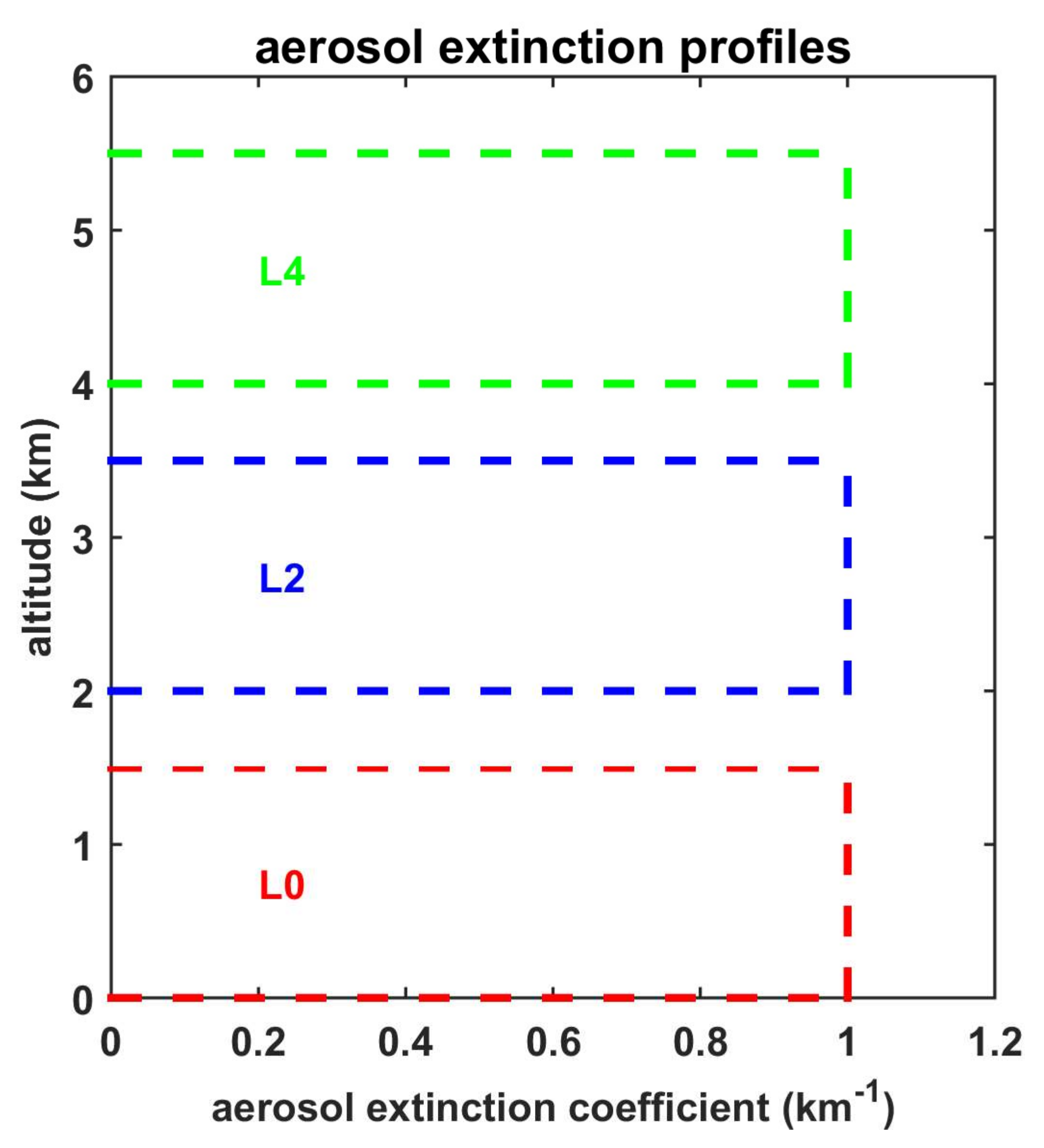
• As a first step, the sensitivity of the solar radiation profile to the altitude of a hypothetical aerosol layer was investigated using artificial aerosol extinction coefficient profiles.
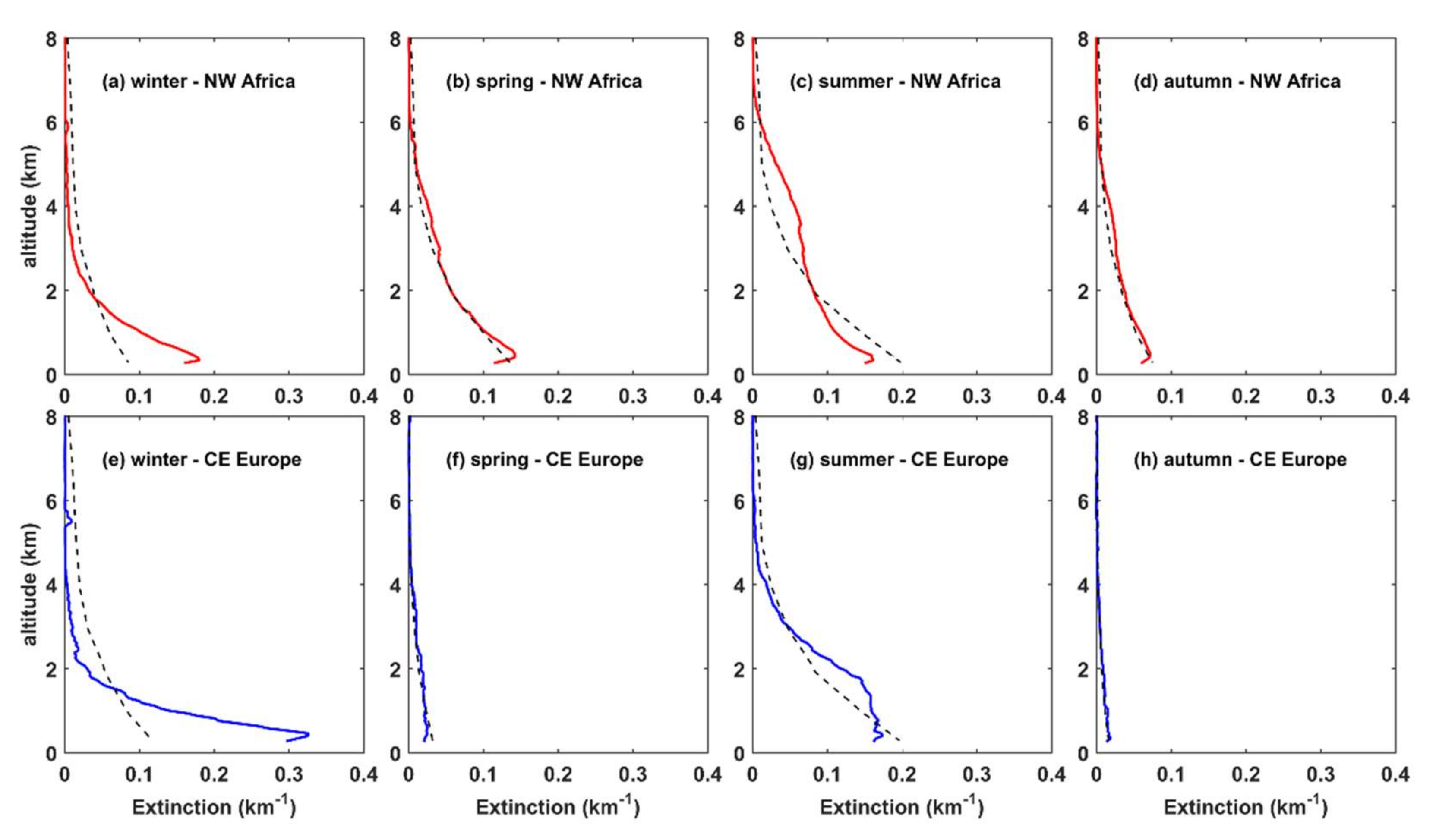
• As a second step, radiative transfer (RT) simulations were performed using aerosol extinction coefficient profiles from the LIdar climatology of Vertical Aerosol Structure for space-based lidar simulation studies (LIVAS) [56], and the results were compared with the results of simulations with the default libRadtran profile [22] which assumed an exponential decrease in the aerosol extinction coefficient with altitude in the troposphere.

The simulations were performed for typical and extreme aerosol conditions and for different European and North African regions. In addition to the AF and HR, we estimated the global irradiance (GI), direct irradiance (DI), downwelling diffuse irradiance (DDI) and upwelling diffuse irradiance (UDI), which are necessary quantities in order to answer the four questions listed in Section 1. Short descriptions of LIVAS and the basic setup for the RT simulations are provided in Section 2.1 and Section 2.2, respectively. A description of the methodology used for the investigation of the role of aerosol profiles on the vertical distribution of solar irradiance is provided in Section 2.3, Section 2.4 and Section 2.5.

2.1. LIVAS

LIVAS is a three-dimensional (3-D) multi-wavelength global aerosol and cloud optical database, which provides averaged profiles of aerosol optical properties at 355, 532, 1064, 1570 and 2050 nm and cloud optical properties at the wavelength of 532 nm [56]. Established on the basis of the Cloud-Aerosol Lidar and Infrared Pathfinder Satellite (CALIPSO) [57]), LIVAS data have been used in various studies for 3D aerosol climatology (e.g., [58,59]). To produce Level 2 (L2) Version 4 (V4) profiles of aerosol and cloud optical properties and layer classification information [60], LIVAS applies a series of quality-assurance procedures [61] prior averaging in order to generate the Level 3 (L3) aerosol profile products, including, among others, vertical profiles of total-aerosol extinction coefficient and AOD at 532 nm. The original LIVAS database is established on a uniform grid of 1°◦ × 1° spatial resolution, with the CALIPSO original vertical resolution, while with respect to the temporal resolution, the aerosol optical properties are provided (1) at the CALIPSO per-orbit level, (2) on monthly means, and (3) on long-term averaged profiles (6/2006–12/2020). However, for the scientific objectives of the present study, the LIVAS total-aerosol extinction coefficient profiles and AODs at 532 nm were generated at two spatial resolutions different from the original one. More specifically, the first option of spatial resolution includes LIVAS optical properties when CALIPSO overpasses Athens, Greece, Cairo, Egypt, and Lampedusa, Italy locations within a horizontal radius of 100 km. For the needs of the present study, the ESA-LIVAS database was established in a 5° × 5° spatial resolution, providing time-averaged profiles of the CALIPSO total-aerosol extinction coefficient at 532 nm for the domains of northwest Africa and central-eastern Europe (more information is provided in Section 2.4 and Section 2.5).

2.2. Radiative Transfer Simulations

The UVSPEC model that is included in the library for the radiative transfer (libRadtran) package [62] was used to perform RT simulations. A number of input parameters were explicitly defined for each of the simulations: total column of water vapor (TCWV), total column of ozone (TCO), surface albedo, columnar aerosol optical properties (the aerosol optical depth (AOD), the single scattering albedo (SSA), the Ångström exponent (AE), and the vertical profile of the extinction coefficient at 532 nm. The latter was then scaled to the value of the AOD at each wavelength. In all cases, the profiles of parameters other than AOD aerosol optical properties (e.g., SSA, AE, asymmetry parameter) were assumed to be constant throughout the atmosphere. A typical, constant value of 0.7 (e.g., [19]) was defined for the asymmetry parameter, as well as a standard CO₂ concentration of 430 ppb. The standard atmospheric profile (standard US atmosphere [63]) was used for all simulations. Thus, the default libRadtran profiles of TCO, TCWV, etc. were scaled to the defined columnar values.

Model outputs were produced for 18 layers between 0 and 8 km, which were denser near the bottom of the atmosphere (BOA) and gradually became sparser with increasing altitude, and at 50 km, considering that differences between radiometric quantities for different aerosol extinction profiles at the 50 km altitude are representative for the corresponding differences at the top of the atmosphere (TOA). Spectral simulations in the range of 280–3000 nm were performed with a step of 1 nm. The extraterrestrial solar spectrum suggested by Kurucz [64] and the sdisort [65] pseudospherical 16-stream approximation of the UVSPEC model were used for the simulations. Simulations were performed separately for the four spectral regions: UVB, UVA, VIS, NIR. For the simulations in the NIR region, absorption was parametrized using the correlated-k KATO2 distribution [66,67]. Although the latter parameterization introduced some additional uncertainty into the simulations compared to a spectral or pseudo-spectral parameterization, the additional uncertainty was negligible for the NIR integral [68].

The produced spectra were integrated in order to calculate and analyze the total irradiance in the four spectral bands (UVB, UVA, VIS, NIR) and the total SW irradiance. The required quantities were finally produced at the model output: DI, GI, DDI, UDI, AF, and HR.

2.3. Sensitivity Study Using Artificial Extinction Profiles

The first step of the study was to perform simulations for five different artificial homogeneous layers of aerosols, with layer bases at 0, 1, 2, 3, and 4 km (hereafter referred as L0, …, L4, respectively) from the surface (assuming that the surface is at mean sea level). Three of the five layers are shown in Figure 1. The width of each layer was 1.5 km. The aerosol extinction coefficient above and below each layer was considered zero. Simulations were performed for combinations of different atmospheric and surface parameters, as well as different aerosol optical properties (see

Table 1. UVSPEC model input parameters.

Property	Values
SZA	20°, 40°, 60°, 80°
AOD (all wavelengths)	0.2, 0.5, 1.0
SSA (all wavelengths)	0.75, 0.95
Asymmetry factor	0.7
AE	0
TCO	350 DU
TCWV	1.3 g/cm2
Surface albedo	0.1, 0.4, 0.8

). For each spectral band, the AOD was considered to be independent from wavelength for the simulations (i.e., AE was set to zero).

For the same sets of parameters and different extinction coefficient profiles, comparisons between the vertical profiles of the different radiometric quantities were performed. In all cases, the results for elevated aerosol layers were compared with the results for L0. This way, it was possible to investigate the effect of different aerosol layer altitudes and understand the physical mechanisms that are responsible for the differences in the profiles of the radiometric quantities.

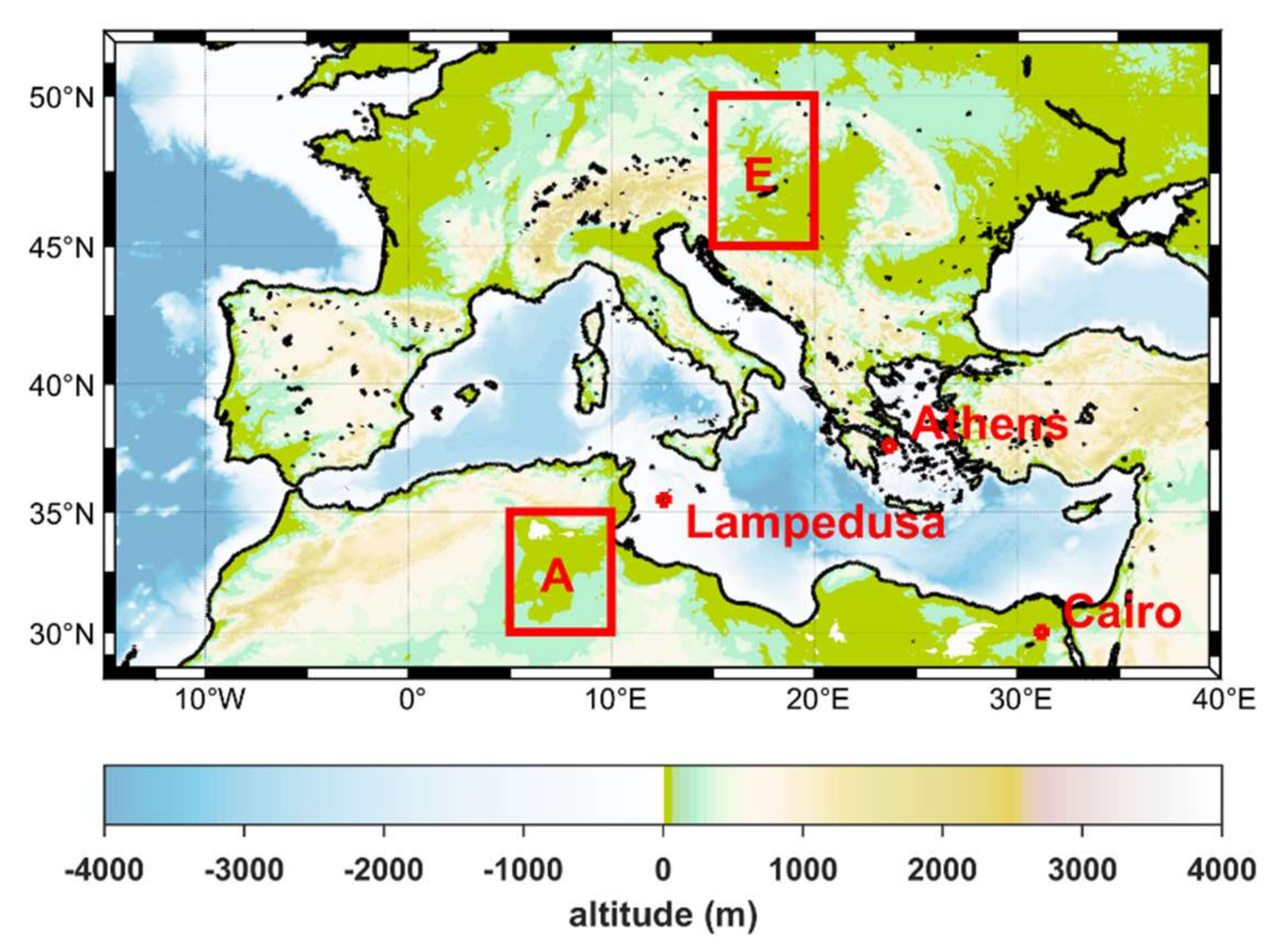
2.4. Simulations Using Theoretical and LIVAS Profiles for Typical Aerosol Conditions

Aerosol extinction profiles at 532 nm from the LIVAS climatology were averaged for two 5° × 5° regions with centers in northwestern Saharan desert, Africa (32.5°N, 7.5°E), and central-eastern Europe (47.5°N, 17.5°E) (see Figure 2), for the period 6/2006–12/2020. In the following, the two regions are referred to as NW Africa and CE Europe, respectively. Accordingly, from the daily LIVAS profiles, monthly averaged profiles were calculated and subsequently averaged again to calculate seasonal profiles for winter (December, January, February; DJF), spring (March, April, May; MAM), summer (June, July, August; JJA), and autumn (September, October, November; SON). Seasonal profiles were used to perform RT simulations. RT simulations were also performed using the libRadtran default profile [22]. RT simulations for each season were performed for both profiles assuming climatological seasonal averages for TCWV, TCO, aerosol optical properties (AOD, SSA, AE), and surface albedo.

Climatological seasonal TCWV from the Copernicus Atmospheric Monitoring Service (CAMS) [69], TCO from the Ozone Monitoring Instrument (OMI) [70], and AOD retrievals at 550 nm from the MODerate resolution Imaging Spectroradiometer (MODIS) onboard the Aqua satellite (Collection 6.1; [71]) were averaged for the same areas and seasons and used for the simulations. The utilized quality assured MODIS-Aqua 550 nm AOD product was obtained by MIDAS dataset [58]. Seasonal climatological averages for the period 2006–2020 were calculated from monthly averaged surface albedo from the Modern-Era Retrospective Analysis for Research and Applications, Version 2 (MERRA-2) climatology [72], and was used for the simulations in VIS and IR. Surface albedo in UV differs significantly from surface albedo in VIS for particular land-surface types such as deserts. Thus, typical values were used [73,74], since large-scale climatological data are not available. Seasonally averaged SSA and AE were calculated from monthly averages, which were derived from the Max Planck Aerosol Climatology version 2 (MACv2) [75] and used for the RT simulations. The above parameters are listed in

Table 2. TCO, TCWV, surface albedo and AOD at 550 nm used in the simulations for NW Africa and CE Europe.

	Winter	Spring	Summer	Autumn
550 nm AOD
NW Africa	0.19	0.35	0.35	0.26
CE Europe	0.07	0.18	0.22	0.13
TCWV (g/cm2)
NW Africa	11.4	14.6	22.3	20.4
CE Europe	9.6	14.4	25.7	17.4
Total ozone (DU)
NW Africa	299.4	318.3	298.4	282.2
CE Europe	333.3	358.6	320.2	287.8
Surface albedo
NW Africa VIS/IR	0.42	0.40	0.41	0.41
NW Africa UVB/UVA	0.10	0.10	0.10	0.10
CE Europe VIS/IR	0.15	0.15	0.15	0.15
CE Europe UVB/UVA	0.05	0.05	0.05	0.05

,

Table 3. SSA used in the simulations for NW Africa and CE Europe. For each spectral band, independence from wavelength SSA was assumed.

		Winter	Spring	Summer	Autumn
NW Africa	UVB	0.84	0.77	0.81	0.80
	UVA	0.85	0.78	0.82	0.81
	VIS	0.93	0.93	0.94	0.93
	IR	0.94	0.96	0.96	0.96
CE Europe	UVB	0.80	0.86	0.87	0.83
	UVA	0.81	0.87	0.88	0.85
	VIS	0.87	0.91	0.92	0.90
	IR	0.86	0.91	0.91	0.89

and

Table 4. AE used in the simulations for NW Africa and CE Europe.

		Winter	Spring	Summer	Autumn
NW Africa	UVB	1.32	0.74	1.04	0.89
	UVA	1.32	0.74	1.04	0.89
	VIS	1.32	0.74	1.04	0.89
	IR	0.65	0.20	0.31	0.30
CE Europe	UVB	1.32	1.52	1.66	1.41
	UVA	1.32	1.52	1.66	1.41
	VIS	1.32	1.52	1.66	1.41
	IR	1.32	1.30	1.40	1.27

.

2.5. Simulations Using Theoretical and LIVAS Profiles for High Aerosol Load

Mediterranean countries are often affected by strong dust events, resulting in high AODs and extinction coefficient profiles that differ significantly from the default libRadtran profile [22]. LIVAS extinction coefficient profiles were interpolated to the coordinates of three Mediterranean sites: Cairo (31.2°E, 30.0°N), Lampedusa (12.6°E, 35.5°N), and Athens (23.7°E, 37.6°N). The (normalized) profiles corresponding to 532 nm AOD > 0.8 were averaged for the period 2006–2018 and used for the RT simulations. Visual inspection of the profiles and back-trajectory analyses of air masses from the HYSPLIT model (https://www.ready.noaa.gov/HYSPLIT.php (accessed on 15 January 2022)) revealed that high AOD was in all cases related with strong dust events. RT simulations were performed assuming typical optical properties for dust-dominated aerosol mixtures (AE = 0.3 and SSA: 0.8, 0.85, 0.95, 0.98 for UVB, UVA, VIS, and NIR, respectively) [17,76] and 550 nm AOD = 1. Extreme dust events where AOD at 550 nm exceeds 1 have been recorded over the Mediterranean Basin (e.g., [77]), but are very rare, while events with AOD of 0.8–1 are more frequent. Thus, AOD = 1 was chosen in order to study the effect of the aerosol extinction profile during strong dust events. In addition to the aerosol optical properties, other model inputs were the annual averages of TCWV, TCO, and surface albedo. The latter quantities were derived from the sources described in Section 2.4 for the period 2006–2018. Climatological annual averages were calculated and used for the simulations. RT simulations were repeated for the same conditions using the default libRadtran extinction coefficient profile [22], instead of the LIVAS profiles. The input parameters for UVSPEC are listed in

Table 5. TCO, TCWV, surface albedo and aerosol optical properties (AOD at 550 nm, SSA, AE) used in the simulations for Cairo, Lampedusa and Athens AOD at 550 nm.

	550 nm AOD	SSA	AE	TCWV (g/cm2)	TCO (DU)	Surface Albedo
Cairo
UVB	1	0.80	0.3	1.66	295	0.05
UVA	1	0.85	0.3			0.05
VIS	1	0.95	0.3			0.11
IR	1	0.98	0.3			0.11
Lampedusa
UVB	1	0.80	0.3	2.03	312	0.05
UVA	1	0.85	0.3			0.05
VIS	1	0.95	0.3			0.08
IR	1	0.98	0.3			0.08
Athens
UVB	1	0.80	0.3	1.85	317	0.05
UVA	1	0.85	0.3			0.05
VIS	1	0.95	0.3			0.11
IR	1	0.98	0.3			0.11

.

3. Results and Discussion

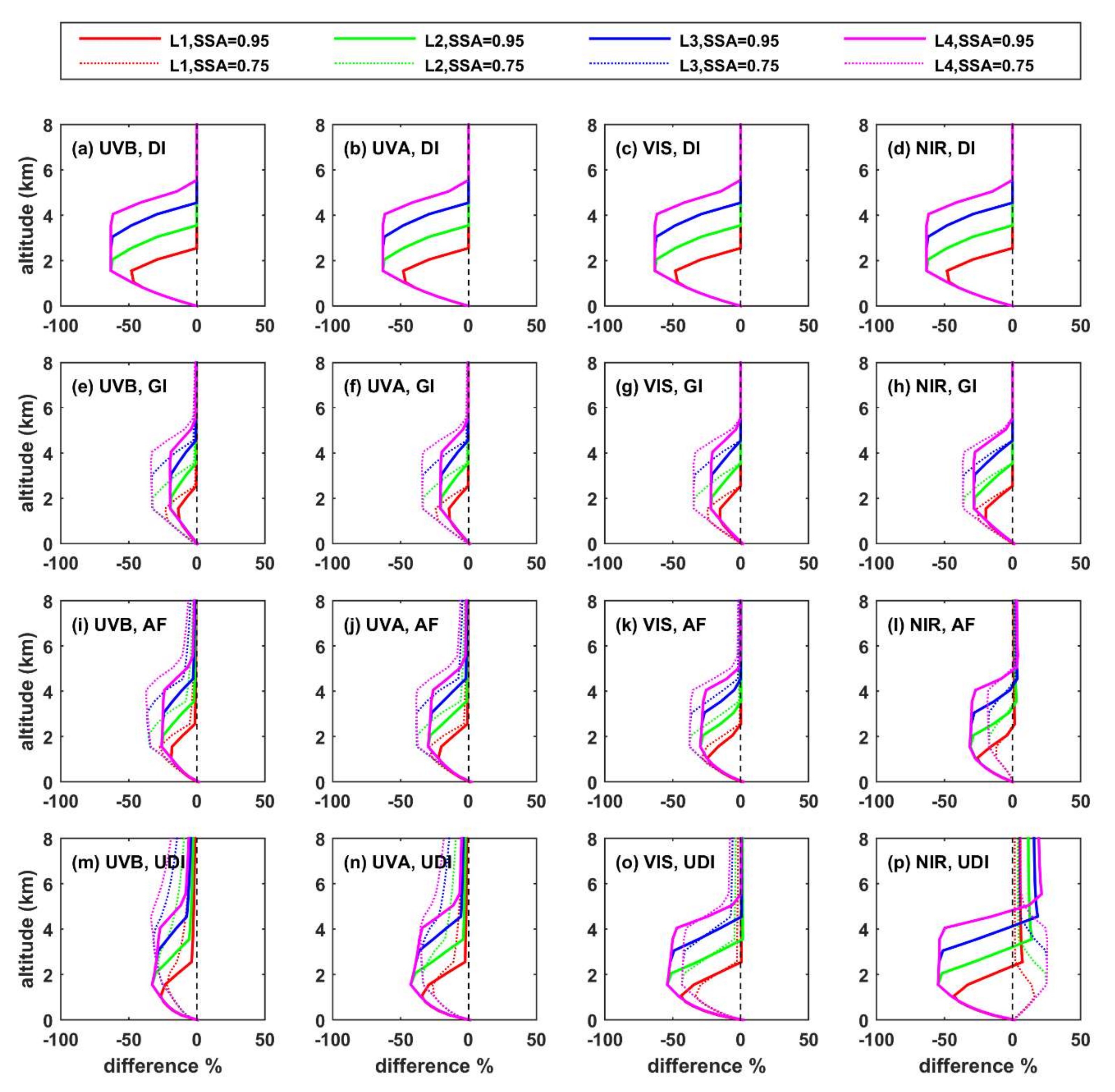
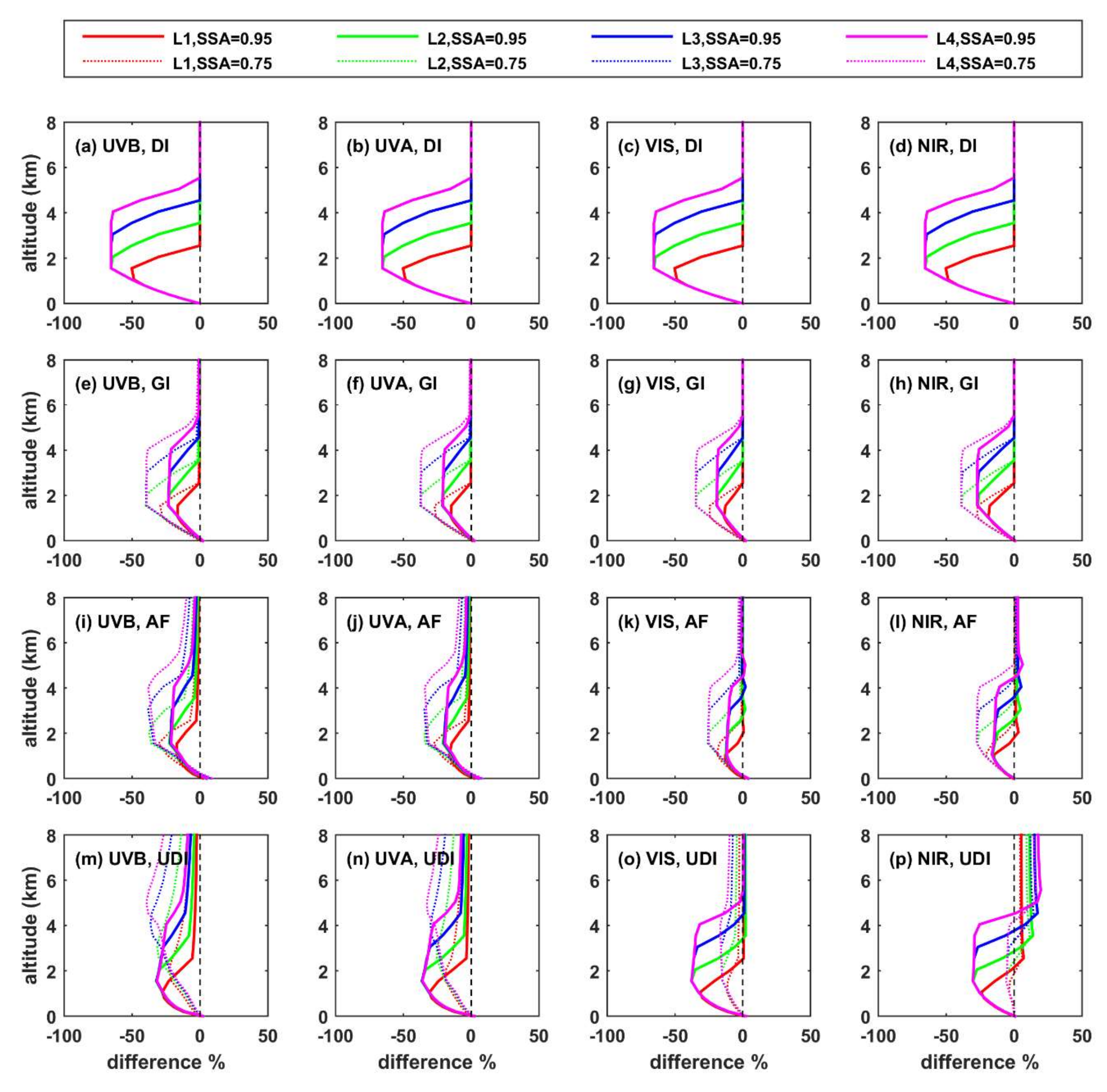
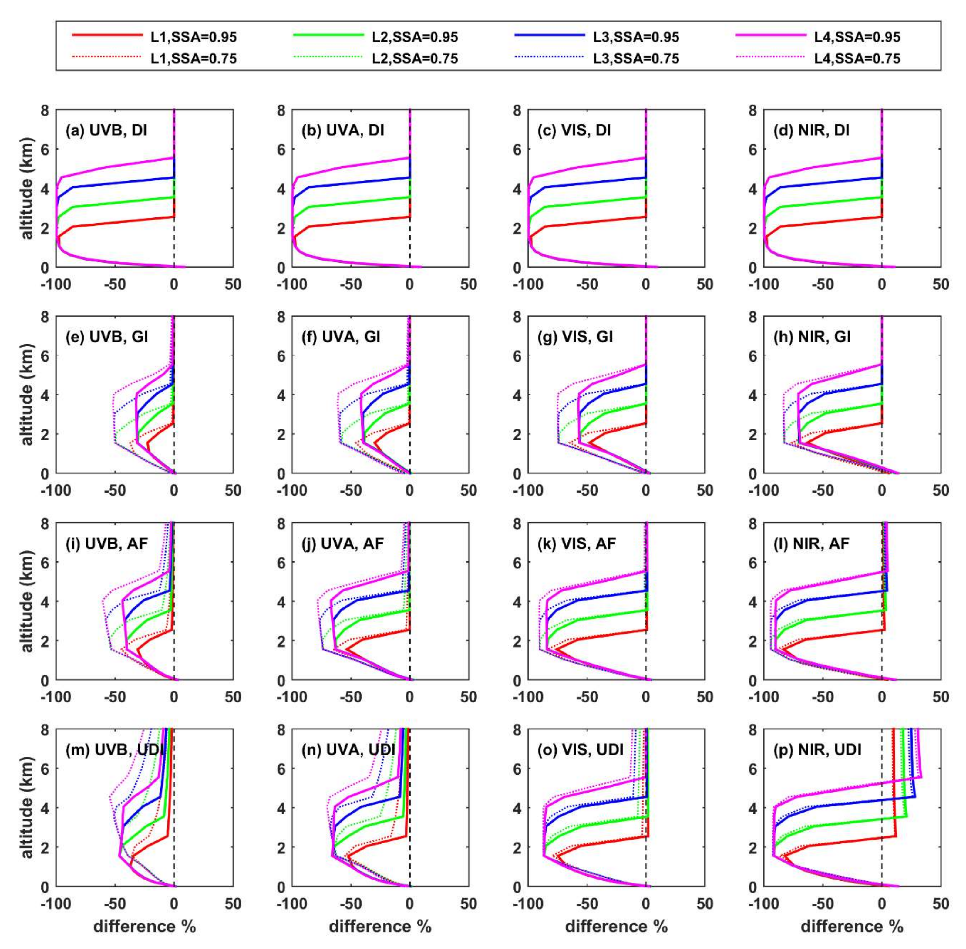
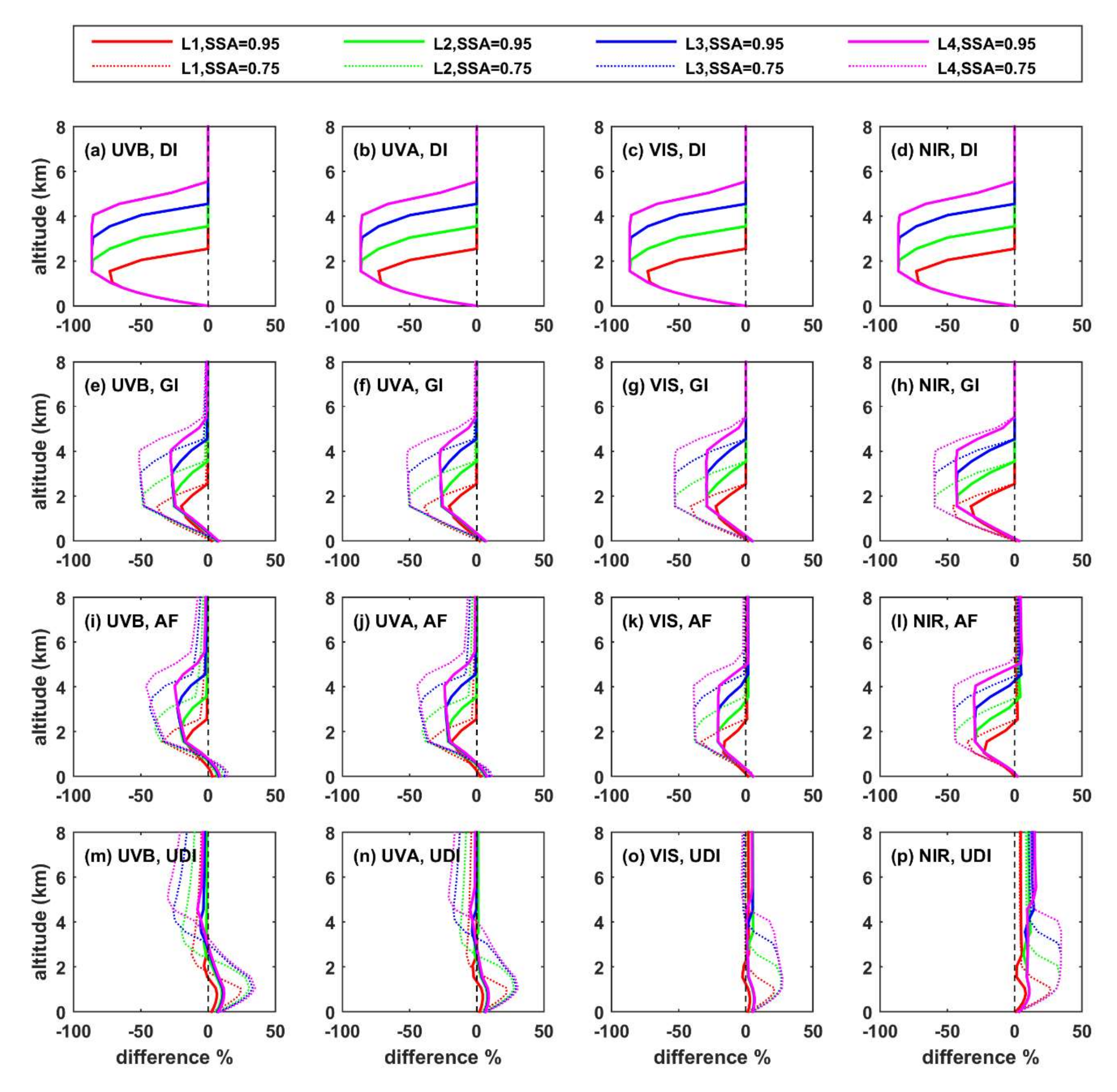
3.1. Altitude of the Aerosol Layer

As described in Section 2.3, the magnitude of the differences in the vertical radiation profiles when the altitude of the aerosol layer changes was investigated using artificial aerosol extinction profiles. Relative differences (%) were calculated between simulations for which all parameters were the same, except the aerosol extinction coefficient profile. The radiation profiles for elevated aerosol layers (L1, …, L4) were compared with the radiation profiles for L0. L0 was used as a reference because it is closer to commonly used climatological profiles, as most of the radiation extinction by aerosols takes place near the surface. Sensitivity of the results to different TCWV was found to be very small even in the NIR (although the profile of NIR changes significantly for different values of the TCWV). Thus, only results for TCWV = 1 g/cm² are presented. Moreover, sensitivity analysis that was performed prior to the simulations revealed that the effect of changes in TCO (within realistic limits) on the results was also negligible. Therefore, all simulations were performed for TCO = 350 DU.

The differences for different radiometric quantities (DI, GI, DDI, UDI, and AF) and spectral regions (UVB, UVA, VIS, and NIR) are presented in Figure 3 and Figure 4. The presented results are for AOD = 1, SZA = 60°, surface albedo = 0.1, TCWV = 1 g/cm², and two values of the SSA: 0.75 and 0.95. The results for the DDI are presented in an independent figure (Figure 4) because of the different scale relative to other quantities. Results for different AOD (0.2 and 0.5), surface albedo (0.8), and SZAs (20° and 80°) are presented in Appendix A and are discussed in the present section.

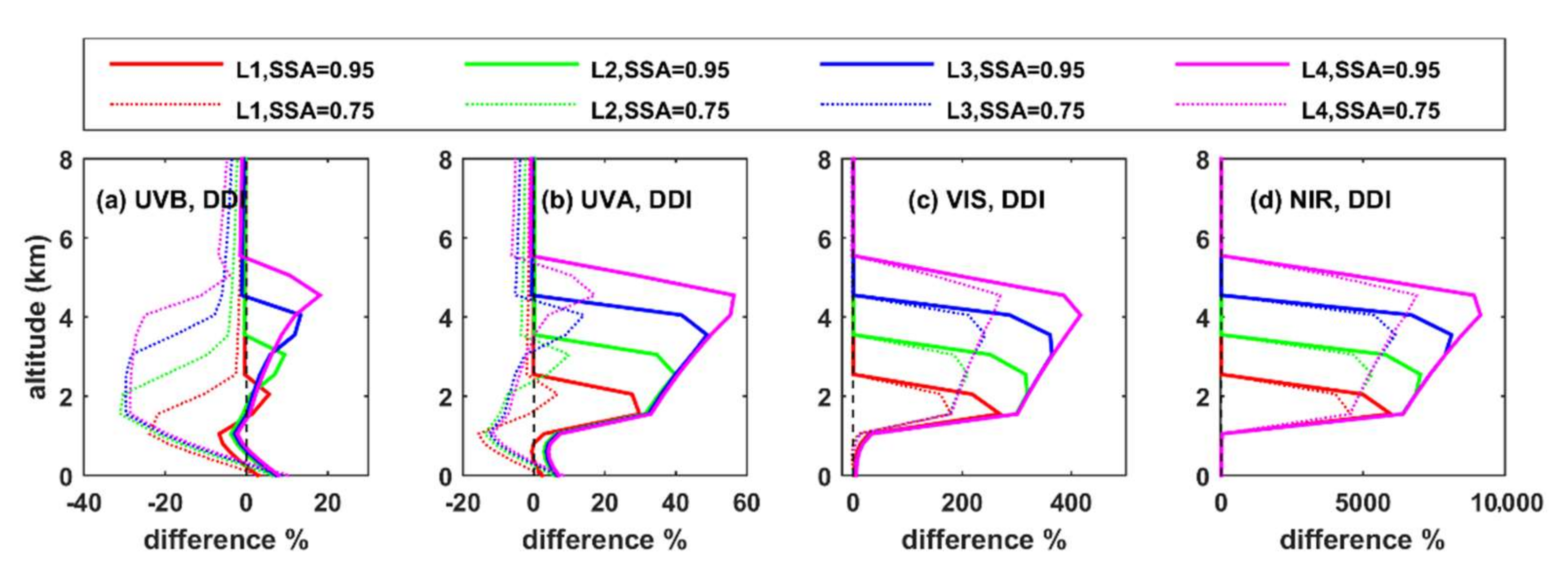
3.1.1. Direct Irradiance

In line with the radiative transfer theory basics, changing the altitude of the layer had the same effect on the DI in all four spectral regions because attenuation of DI depends solely on the AOD, which was assumed to be constant in all spectral bands. When simulations were performed with the aerosol layer at a higher altitude instead of L0, then the DI gradually decreased from the top to the bottom of the elevated layer, while the difference with respect to the irradiance for L0 gradually increased (up to ~86% at the bottom of the elevated layers when the layer base was higher than the top of L0). Then, at the top of L0 the differences gradually tended to zero, and finally there was no change in the amount of DI that reached the surface. Decreasing/increasing the SZA or the AOD for the simulations led to smaller/larger differences in DI between the layers (Figure A1, Figure A2, Figure A3, Figure A4 and Figure A5). The results for DI were independent from the changes in SSA and surface albedo.

3.1.2. Diffuse Downwelling and Upwelling Irradiances

Changes in diffuse irradiance strongly depend on solar spectral region and the SSA. The presence of aerosols leads to increased scattered (downwelling and upwelling) irradiance relative to aerosol-free atmosphere. Additional scattering and absorption of solar radiation with respect to aerosol-free atmosphere takes place inside the layer of aerosols and also affects the distribution of photons above and below the layer.

Downwelling Diffuse Irradiance

For scattering aerosols (SSA = 0.95), the increase in the DDI due to the presence of an elevated aerosol layer (with respect to the corresponding DDI for L0) begins at the top of the layer and becomes maximum near the middle of the layer. The maximum difference is larger for L4 and gradually becomes smaller for lower-altitude layers. In an aerosol-free atmosphere, the DDI would increase with decreasing altitude. Rayleigh scattering is more intense for shorter wavelengths. At UVB wavelengths the diffuse component of the downwelling irradiance is already strong between 4 and 5.5 km even in an aerosol-free atmosphere, while at NIR wavelengths there is nearly zero DDI at the same altitude under the same conditions. Thus, the same absolute increase in DDI due to the presence of aerosols would lead to a much larger relative increase in NIR relative to UVB. For example, for L4 the maximum increase is ~10% for UVB and ~10,000% for IR. The relative increase gradually becomes weaker below about the middle of the elevated aerosol layer. Below 1 km, UVA DDI for elevated aerosol layers is smaller with respect to the DDI for L0 (for SSA = 0.95). For UVB, differences in DDI (DDI for an elevated aerosol layer—DDI for L0) switch from positive to negative at a distance of a few hundreds of meters below the base of the elevated aerosol layer.

When aerosols are more absorbing (SSA = 0.75), the magnitude of differences between the DDI for elevated aerosol layers and the DDI for L0 is in all cases smaller compared to more scattering aerosols (SSA = 0.95). In UVA, the DDI is larger at the altitude of the elevated layer and smaller in the rest of the atmosphere, while in UVB, the DDI is smaller even at the altitude of the elevated aerosol layer. This is because absorption of the scattered irradiance coming from Rayleigh scattering dominates over excessive scattering by aerosols when the aerosols are at higher altitudes relative to L0. It is interesting that in UVB and UVA, DDI also decreases above the elevated aerosol layers, with the decrease being larger for more elevated layers (i.e., maximum for L4). This is because when the layer of aerosols is higher, it absorbs more photons before they interact with the denser atmosphere below the layer. If the layer was lower (e.g., L0 instead of L4), a fraction of these photons would be backscattered before entering the layer of aerosols. In simple words, more photons interact with aerosols, and subsequently more photons are absorbed when the layer is higher. A fraction of the photons absorbed in the elevated layer would have been absorbed anyway in L0. However, another part would have been backscattered towards the TOA. Differences in the number of photons that reach the surface are in both cases smaller, leading to differences of a few percent at the BOA.

Decreasing the AOD suppresses the differences without changing their direction (Figure A6 and Figure A7). Changing the SZA, however, can also have an impact on the direction of the differences, leading to “less positive” differences for larger SZAs (Figure A8 and Figure A9). When the surface is highly reflective (e.g., surface albedo = 0.8, Figure A10), the differences are slightly more positive (by ~5–10%) for UVB and UVA relative to those for surface albedo = 0.1, for altitudes between the bottom of the elevated layer and the BOA. Inside and above the elevated layer, differences are much smaller with respect to the corresponding lower surface albedo cases. This is possibly because the aerosol layer and the reflective terrain enhance the scattering toward the BOA (the former) and the TOA (the latter), leading to an increased number of photons between the aerosol layer and the surface. At VIS and NIR wavelengths, this effect is minor relative to UVB and UVA because of the less efficient scattering by air molecules, and the corresponding differences (for high and low surface albedo) are very small.

Upwelling Diffuse Irradiance

At NIR wavelengths the scattered irradiance in the atmosphere is negligible in the absence of aerosols. Thus, adding a layer of aerosols leads to more UDI inside and above the layer. Increasing the altitude of the layer leads to more UDI at the TOA, as the scattered photons have fewer chances to interact with absorbing gases (mainly water vapor). Thus, when comparing the UDI profiles for elevated layers (L1, …, L4) and L0, the difference is always positive above about the middle of the elevated layer. For SSA = 0.95, the difference is negative below the middle of the layer, while for SSA = 0.75, it is positive, which means that the NIR UDI increases between the elevated aerosol layer and the BOA. For scattering aerosols, it is easy to understand that when the layer is lower, there is more UDI at lower altitudes. However, when absorbing aerosols are low in the atmosphere (L0), it is possible that combined absorption of the NIR by gases and aerosols is stronger than the absorption when aerosols are higher in the atmosphere. This is because, at the SZA of 60°, some of the photons that have been scattered at a higher altitude go through shorter optical paths (relative to being scattered near the surface) as they propagate toward the surface, because they move “more vertically” (i.e., at zenith angles smaller than 60°) in the atmosphere. Thus, they have fewer chances to be absorbed, and more chances to be reflected toward the TOA. It is possible that the combination of the two phenomena described above leads to more NIR UDI when the aerosol layer is higher. This is not, however, the case for different SZAs (e.g., SZA = 20° or SZA = 80°), for which the differences in NIR UDI are negative below the elevated layer, even for absorbing aerosols (Figure A3 and Figure A4). For SZA smaller than 60°, that happens because the difference in the path of the photons does not change as significantly as for SZA = 60°. For SZA = 80°, the attenuation of the NIR irradiance in the aerosol layer is so strong that differences below the layer are again negative. Very high surface albedo (e.g., surface albedo = 0.8) leads to increased UDI below the base of elevated aerosol layers (compared to UDI at the same altitudes for aerosols at L0) even for SSA = 0.95 (Figure A5). This is possibly because many NIR photons are reflected at the surface (towards the aerosol layer) and then scattered in the layer (towards the surface), and this process is repeated multiple times for a fraction of the photons. It should be kept in mind that the above discussion refers to a default typical asymmetry parameter of 0.7. Changing the asymmetry parameter can lead to different results.

Absorption of the UVB, UVA and VIS radiation in the troposphere is generally weak (under usual conditions) with respect to the absorption of NIR radiation. Aerosols at any altitude enhance the NIR UDI inside and above the layer. As the altitude of the layer increases, it absorbs and scatters back to the surface part of the UDI that enters the base of the layer from below. Thus, for UVB, UVA, and VIS, an elevated aerosol layer results in less UDI above, inside, and below the elevated layer with respect to the UDI inside and above L0. The differences are more significant above the elevated layer for more absorbing aerosols. For SSA = 0.95, the absolute differences increase gradually from the top to the bottom of the elevated layer, then remain relatively stable between the base of the elevated layer and the top of L0 and again decrease until the surface. For UVB and UVA (where Rayleigh scattering is more intense relative to VIS) when SSA = 0.75, the absolute difference is maximum inside the aerosol layer and then decreases (faster below the top of L0) until the surface. Decreasing the AOD suppresses the differences (Figure A1 and Figure A2) without, however, significantly changing their relative distribution in the atmosphere. Similarly, changing the SZA (Figure A3 and Figure A4) mainly affects the magnitude of the decrease.

When an elevated aerosol layer is above very reflective terrain, enhanced multiple scattering leads to a significant increase in the UDI between the layer and the surface (especially at shorter wavelengths). Increasing the altitude of the layer reduces the UDI above the layer with respect to an aerosol-free atmosphere, more than it does over low-albedo terrain. The latter reduction becomes stronger as the absorption efficiency of the aerosol layer increases. Thus, comparing UDI for an elevated aerosol layer with UDI for L0 (Figure A5) resulted in positive differences between the bottom of the elevated layer and the surface. For UVB and UVA, the differences were negative above the altitude of the bottom of the elevated aerosol layer. They became more negative with increased absorption efficiency of the aerosols and increased altitude of the layer. For VIS, the differences were (as they were for IR) positive even above the altitude of the bottom of the elevated layer.

3.1.3. Global Irradiance

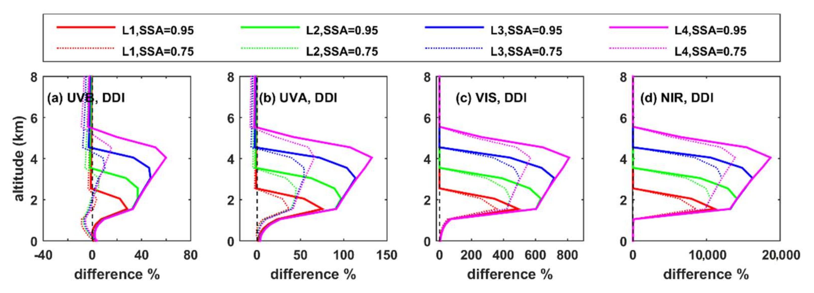
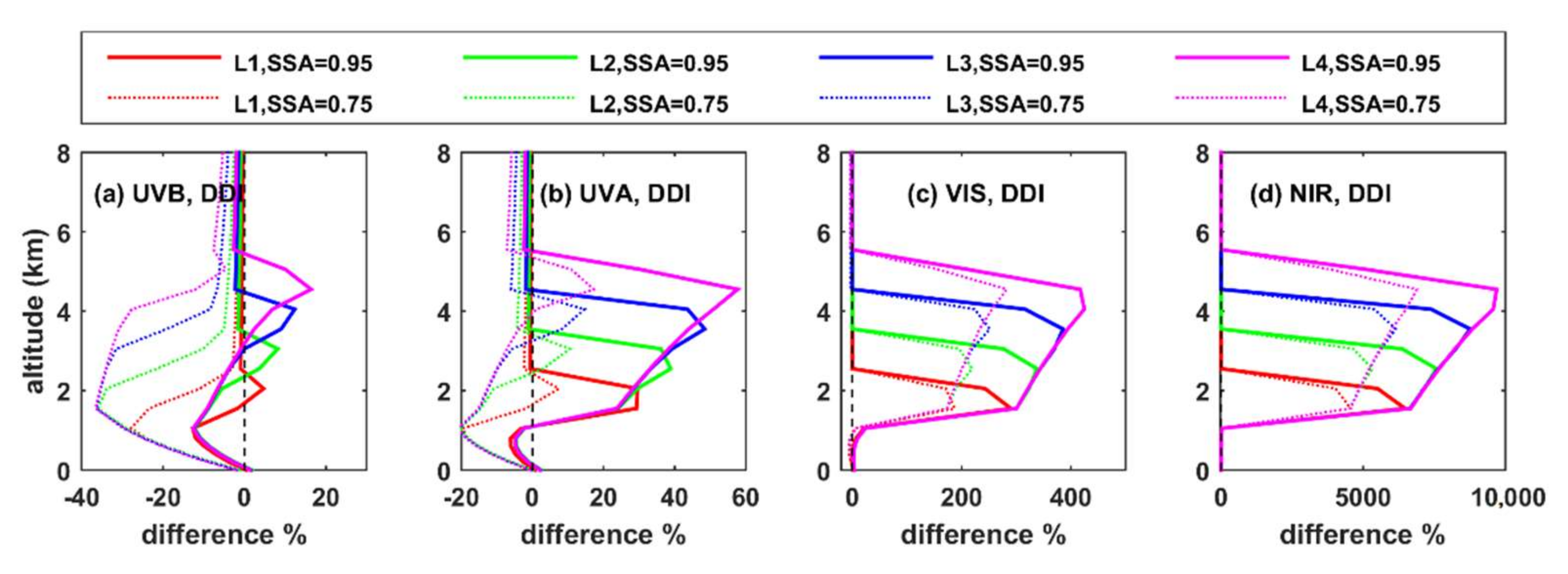
The global irradiance (GI) is the summary of the DI and the DDI. Thus, differences due to changes in the altitude of the aerosol layer depend on the differences in DI and DDI, and on the contribution of each component to the GI. The contribution of DI is more significant for longer relative to shorter wavelengths (because longer wavelengths are scattered less effectively by air molecules) and becomes more significant as SZA decreases. In the UVB region, the diffuse component of the downwelling irradiance is already very strong in the GI at 60°, even above the aerosol layer. As wavelength increases the relative contribution of the direct component becomes more significant, and for the NIR, the direct component becomes dominant. Thus, despite the very large differences between different spectral regions regarding the effect of altitude on DDI, the results for GI were very similar. For SSA = 0.95, the differences between the bottom of the elevated layer and the top of L0 were −35–−45%, while for SSA = 0.75, the corresponding differences were about −60%. Changing the AOD, the SZA, or the surface albedo (Figure A1, Figure A2, Figure A3, Figure A4 and Figure A5) affects the absolute differences, but not their direction or distribution. However, at very high SZAs, the absolute differences are larger (in percent) for larger wavelengths (Figure A4), but they correspond to low absolute GI values.

3.1.4. Actinic Flux

Increasing the altitude of the aerosol layer leads to decreased actinic flux between the elevated layer and L0. As for GI, the decrease is constant between the top of L0 and the bottom of the elevated layer and does not depend on the altitude of the elevated layer unless its bottom is below the top of L0. At SZA = 60° and for SSA = 0.95 and surface albedo = 0.1, the decrease was ~40% for UVB and became larger with increasing wavelength, up to ~55% for NIR. Under the same conditions but for SSA = 0.75, the decrease was larger for UVB (~60%) and became smaller for increasing wavelength (it was ~45% for NIR). As the SZA increases, the effect of changing altitude of the aerosol layer becomes more significant for longer wavelengths. For example, at 80°, the differences between the bottom of the elevated aerosol layer and the top of L0 were of the order of −90% for NIR, while for UVB they were similar to the differences for 60° (Figure A4). Over high albedo surfaces, the effect of changing altitude of the aerosol layer is less significant (compared to the same changes over low albedo surface), especially for highly scattering aerosols (Figure A5). As discussed earlier, this is because increasing the altitude of the aerosol layer leads to decreased DI, but at the same time to increased diffuse irradiance below the layer (with respect to what happens at the same altitudes in the atmosphere for aerosols at L0).

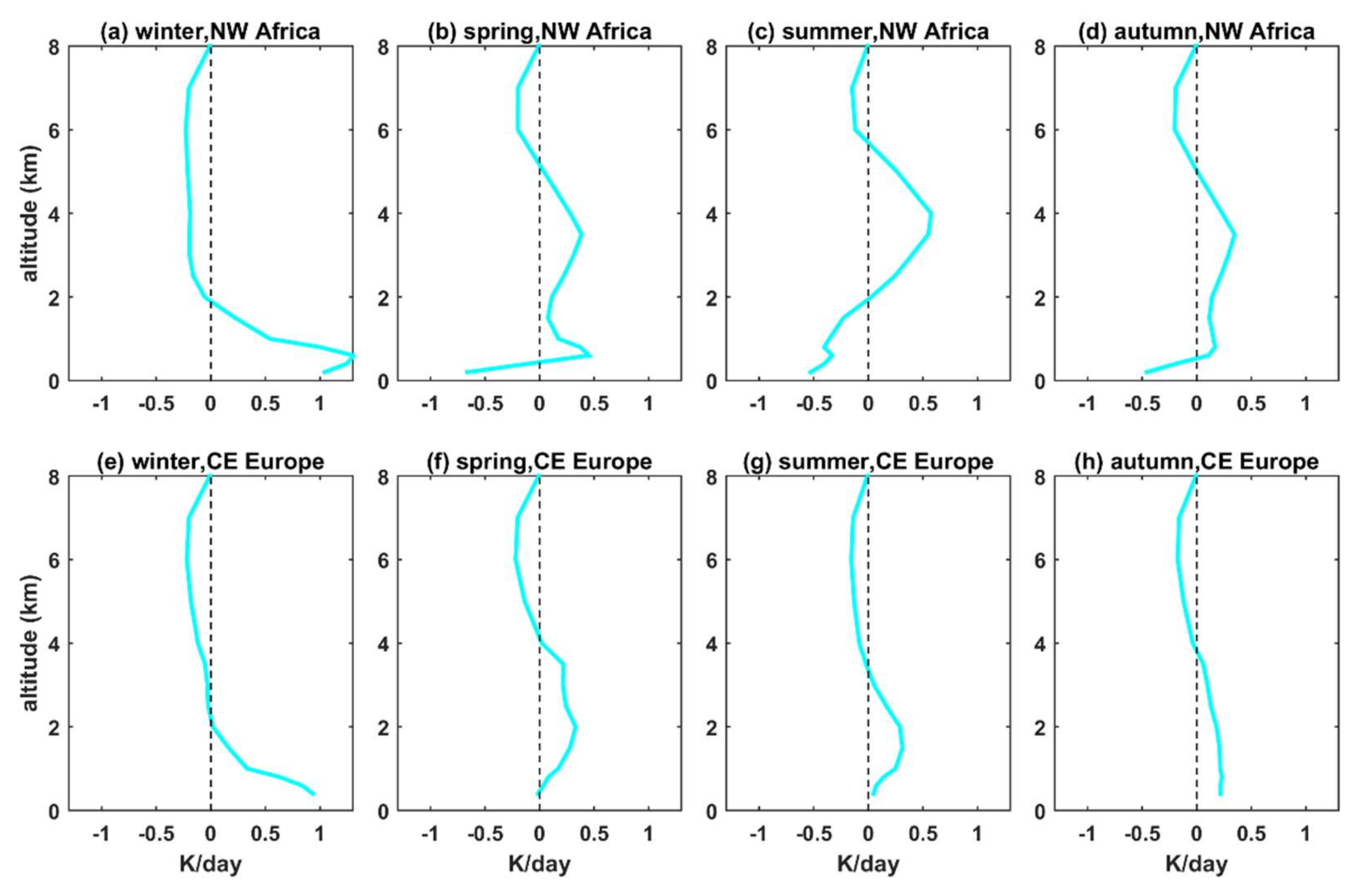
3.1.5. Heating Rates

Differences in HR depict differences in the net flux of irradiance (i.e., the difference between the ingoing and outgoing irradiance at a specific altitude). In the absence of aerosols, this quantity is very small (below 0.1 K/day) for the SW radiation, which explains the very large differences presented in Figure 5. Changes in UVB and UVA play a minor role in the overall changes in the HR of the SW irradiance, and the main contribution comes from radiation in the VIS and NIR regions. Thus, changes in the HR for the total SW radiation are discussed in this section.

HR increases significantly inside, and a few hundreds of meters above and below, the elevated aerosol layers and decreases below the layers with respect to the heating rate for L0 (Figure 5). The increase inside the layer was very large, while the decrease below the layer gradually reached values between 90% and 100% at the altitude of 1.5 km (i.e., the top of L0). The increase inside the layer becomes larger as the layer altitude increases, and further increases for more absorbing aerosols and larger SZA. Increasing the surface albedo leads to very small changes (small suppression of the differences) in the results.

3.1.6. Top and Bottom of the Atmosphere

In most climatic studies, default aerosol profiles are used which commonly assume an exponential decrease in aerosol extinction (with aerosols concentrated in the first 1–2 km from the surface). In many cases, this assumption does not affect the modeled irradiance at the BOA and the TOA significantly (e.g., [23]). However, as shown in the following section for high aerosol loads and under certain conditions (e.g., high SZA or high surface albedo, aerosol layers at very high altitudes), this assumption can result in non-negligible errors in the simulations of the GI at the BOA or the UDI at the TOA when a large fraction of the aerosols is located at higher altitudes (e.g., at 3 or 4 km). In this section, the effect of the altitude of the aerosol layer on GI, at the surface, and UDI at the TOA are discussed for AOD = 1.

BOA

Differences (in %) in the GI for the four spectral bands as it was simulated for aerosols at higher altitudes (L1, …, L4) and aerosols at L0 are presented in Figure 6. Below SZA = 60° and for low surface albedo, the altitude of the aerosol layer had a small impact on the GI that reached the surface, since differences were in all cases below 5%. For SZA = 80,° the differences were larger, up to 15%, mainly for UVA and NIR. For UVA, increasing the altitude of the layer led to increased absorption by absorbing (SSA = 0.75) aerosols. For L4, the reduction was nearly 8% with respect to the UVA at the BOA for L0. A possible explanation is that the direct beam that enters L0 is significantly weaker than the direct beam that enters L4. At such large SZA, the optical path inside the layer is longer for photons of the direct beam relative to scattered photons. Thus, when the aerosol layer is higher, absorption of UVA irradiance by aerosols is stronger. For UVB, the corresponding reduction is smaller because at high SZA (above 60°) the contribution of the direct component is already weak relative to the contribution of the scattered component of GI at 5.5 km. In the VIS and NIR regions, although the direct component is stronger than in UV, the photons are scattered less effectively in the atmosphere. Thus, in aerosol-free skies, the direct component of VIS and NIR GI was similar at 1.5 km and 5.5 km. In NIR, the GI at the BOA at SZA = 80° increased with increasing altitude of the aerosol layer (by 12–14% for L4), for both absorbing and reflective aerosols. This is possibly because scattering of the NIR at higher altitude at such large SZA results in a reduced optical path for a significant fraction of the scattered photons as they propagate “more vertically” below the aerosol layer, moving towards the surface, and are thus absorbed less effectively by atmospheric molecules (mainly by water vapor).

The altitude of the aerosol layer plays a more significant role over highly reflective surfaces, especially when Rayleigh scattering is strong (i.e., in the UVB and UVA regions). The global irradiance at BOA increases with increasing aerosol layer altitude, by up to 15% in the UVB for L4 and small SZA. When the layer of aerosols is inside denser atmosphere (i.e., near the surface) the photons follow longer paths in the layer (due to multiple Rayleigh scattering) with respect to elevated aerosol layers. This phenomenon is intensified over reflective surfaces due to multiple interactions of the photons with the surface, the dense atmosphere, and the aerosol particles. If the layer constitutes absorbing aerosols, then increased absorption leads to even larger differences between GI at the BOA for elevated aerosol layers and L0, and up to 15% for L4. Longer wavelengths are scattered less effectively in the atmosphere, which is the reason for the very small (below 3%) differences between Figure 6e,f (for reflective and absorbing aerosols). Rayleigh scattering in the NIR is negligible; thus, the corresponding differences between panels 6 g and 6 h are nearly zero.

Changes in total irradiance (panels 6i and 6j) due to different altitude of the aerosol layer are determined by changes in the VIS and the IR. For increasing altitude of the aerosol layers, the total GI at BOA increases. The increase was smaller than 5% for SZAs below 60° and larger for SZA = 80°. The increase was similar for L2, L3, and L4, at 7–8%. Changing the surface albedo has negligible impact on total GI at the BOA. It must be mentioned that in realistic conditions, the AΕ is larger than 0, and subsequently, the effect of aerosols is larger at shorter wavelengths, which means that the contribution of changes in the NIR to the changes in the total GI would be less significant than the contribution of NIR in the results presented in panels 6i and 6j.

TOA

As shown in Figure 7, changing the altitude of the aerosol layer has a very small impact on UDI in UVB, UVA, and VIS at the TOA when aerosols are highly scattering (SSA = 0.95). In all of these cases, differences in the UDI were well below 5% for different aerosol layer altitudes. This was not the case, however, for NIR, in that differences in the UDI increase with increasing altitude of the aerosol layer. In the latter case, the magnitude of increase depended on surface albedo and SZA and reached 33% for L4 and surface albedo = 0.1. For UVB, UVA, and VIS, aerosols (with SSA = 0.95) play a role that is similar to that of the atmospheric molecules: they scatter and redistribute photons. Thus, the altitude of the aerosol layer does not play a very significant role regarding the UDI that exists in the atmosphere. In contrast, NIR is weakly scattered by atmospheric molecules and is mainly absorbed by water vapor. NIR radiation is, however, scattered by aerosols. Part of the scattered NIR radiation then moves towards the TOA. When the aerosol layer is higher, absorption of the upwelling NIR by water vapor is weaker (due to the smaller optical path), and more UDI reaches the TOA. This effect is weaker over highly reflective terrain and small SZAs (panel 7 h), because in such cases, NIR that has been reflected at the surface constitutes a significant fraction of the UDI.

For absorbing aerosols (SSA = 0.75), the results for the NIR are similar to the results for scattering aerosols (SSA = 0.95). However, absorbing aerosols induce more significant differences in UVB, UVA and VIS relative to scattering aerosols. When aerosols are low in the atmosphere (i.e., L0) the backscattered photons (due to Rayleigh scattering) at altitudes above 1.5 km do not interact with aerosols. However, if the aerosol layer is higher, then backscattered photons coming from higher altitudes in the troposphere will also interact with the aerosols and some of them will be absorbed. Thus, increasing the altitude of the aerosol layer leads to reduced UDI at the TOA. Over highly reflective terrains, the UDI also comprises photons that have been reflected by the Earth’s surface. The altitude of the layer does not significantly affect the percentage of the latter photons that reach the TOA. Thus, the decrease is weaker for surface albedo = 0.8 relative to surface albedo = 0.1.

Although for different spectral regions, changing the altitude of the layer may induce large differences in the UDI at the TOA, the differences are generally below 15% for total UDI. Total UDI increases with increasing altitude of the aerosol layer, mainly for reflective aerosols. As in the previous section, it should be mentioned again that in realistic conditions, the Angstrom exponent is above zero, which means that the results for total UDI would be closer to the results for VIS compared to the results presented in panels 7i and 7j.

3.2. Effect of Extinction Coefficient Profile for Typical Aerosol Conditions

The methodology used in this section has been described in Section 2.4. The differences between the seasonal total-aerosol extinction coefficient (at 532 nm) profiles from LIVAS and the libRadtran default profile [22] (both scaled to the seasonally averaged AOD at 350 nm) for the two regions are presented in Figure 8. The profiles used to calculate the differences are shown in Appendix A (Figure A11).

The different characteristics of aerosols over the two regions lead to quite different patterns in the extinction coefficient profile differences. Over CE Europe, continental aerosols constitute a significant fraction of the aerosol mixture, while over NW Africa, dust plays a very significant role. The differences in the vertical profiles of the AF are presented in Figure 9. In all cases shown in Figure 9, differences are much larger in the UVB and UVA regions relative to VIS and NIR, mainly because the AOD increases with decreasing wavelength, and thus differences in the extinction coefficient profiles become larger. Given that differences in the VIS and NIR AF are very small, the results are discussed only for UVB and UVA in the following. As expected, differences in AF at the BOA were in all cases small, below 3%.

In winter, for both areas, aerosol extinction was underestimated below ~1.5 km and overestimated above the same altitude when the default profile was used for the simulations. Thus, the patterns of differences in AF profiles were similar for the two regions. For UVB and UVA, a maximum increase on the order of 10% was found between 1.5 and 2 km. Less scattering and absorption by aerosols above 1.5 km allows more photons that are moving towards the surface to reach the specific altitude. At the same time excessive scattering by aerosols near the surface leads to more upwelling photons at the altitude of 1.5 km. Thus, the increase is maximum at the particular level.

For CE Europe, the pattern of differences between the default and measured vertical profiles of aerosol extinction coefficient were as follows. Negative differences (i.e., overestimation by the default profile) appear above an altitude that ranges from ~2 km in winter to ~4 km in spring. Then, the differences become positive. In spring and summer, the differences approach zero near the surface. For the reasons discussed above, for all seasons, the corresponding differences in UVB and UVA AF are largest near the altitude of change from negative to positive differences in the aerosol extinction coefficient. Maximum differences in AF are small, at 5–10%, while near the surface the differences are even smaller, below 5%.

For NW Africa, there is a stronger seasonal dependence on the extinction coefficient differences relative to CE Europe. In spring and autumn, the differences are negative above 5–6 km, and positive below, approaching zero at about 2 km. The corresponding differences in AF are positive, with a maximum of ~5% near the altitude where the extinction coefficient differences change from negative to positive (i.e., at 5–6 km). In summer, differences in the extinction coefficient are again negative above ~6 km and positive below. Then, the differences become negative again below 2 km. Differences in UVB and UVA AF are in this case positive above 4 km, and negative below. Absolute maxima in the positive and negative values were spotted at 5 km and 2 km, respectively. This was because, when the LIVAS profile was used for the simulations instead of the default, more downwelling photons reached the altitude of 6 km. Then, the excessive interaction between aerosols and photons in the layer between 2 km and 6 km led to decreased AF below about the middle of the layer.

At lower SZAs, differences become very small (Figure A11), while at larger SZAs (Figure A12), differences in the atmosphere increase, especially for UVA. For example, at 80° differences in the atmosphere reach 20%. At such large SZA, relative differences correspond to small absolute differences, and their impact on photochemical processes is less significant.

In the case of the HR profiles (Figure 10), differences closely follow the differences in the extinction coefficient profiles. Maximum absolute differences in HR were 0.5–1 K/day for SZAs below 60° and became smaller for larger SZAs. Largest differences, of ~1 K/day, were found in winter near the surface for both regions. In summer, using the default profile led to an underestimation of atmospheric heating by SW radiation at ~4 km over NW Africa by ~0.5 K/day. It is clear from these results that even for typical aerosol conditions, the use of a default profile can lead to significant uncertainties relative to the atmospheric heating or cooling due to the interaction of SW radiation with aerosols.

In Figure 11, the differences in the GI at the BOA are presented for each region and each season of the year. In all cases the differences were below 3%, and especially for VIS and NIR, they were in many cases below 0.5%. Given that more than 85% of total SW irradiance is in the VIS and NIR regions, changes in SW GI were also close to zero. These results confirm that for typical aerosol conditions, using a more realistic profile instead of the default is not necessary for the study of the GI at the Earth’s surface.

Differences in UDI at the TOA are presented in Figure 12. Differences are positive for UVB and UVA, nearly zero for VIS, and negative for IR. Given that aerosol extinction is generally overestimated by the default profile at higher and underestimated at lower altitudes in the atmosphere, this result was expected based on the analyses performed in Section 3.1. Except for very high SZAs (i.e., 80°), differences were smaller than 3%. Changes in SW irradiance (not shown in the graph) were very close to changes in VIS, i.e., between 0 and 1%. Thus, the results presented in Figure 12 denote nearly zero change of the modeled SW UDI when a more realistic extinction profile is used for typical aerosol conditions with respect to the default profile.

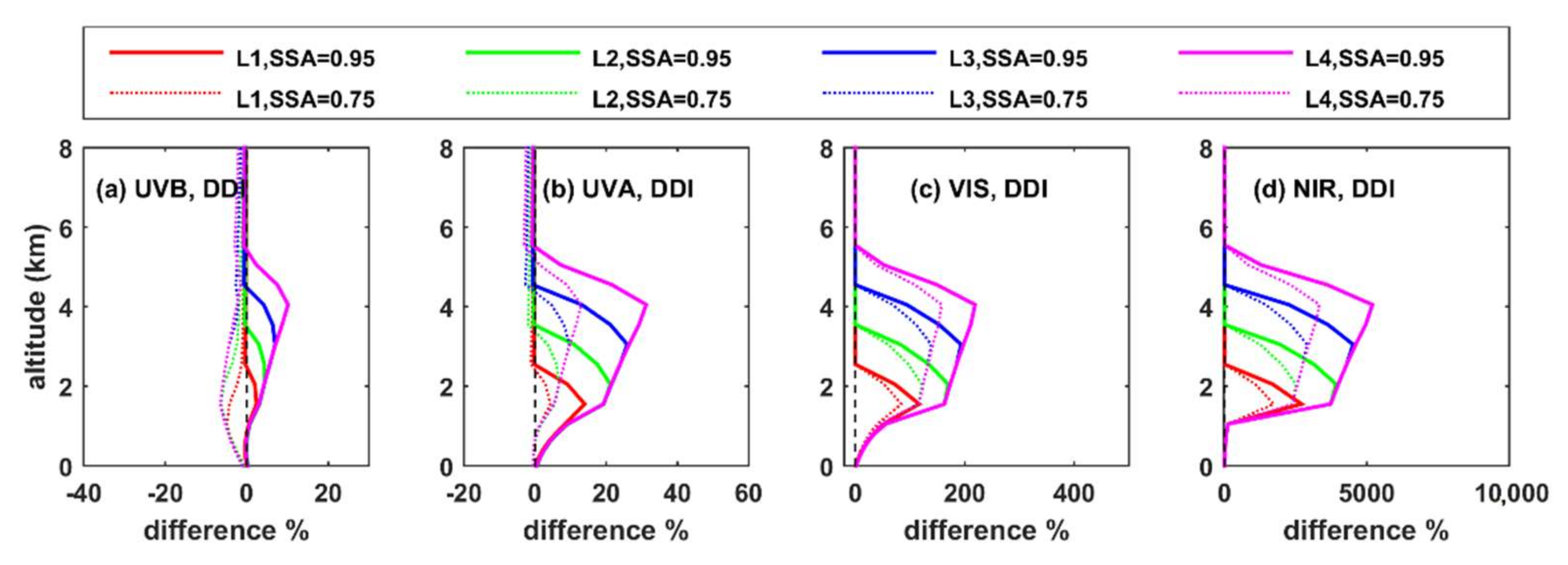
3.3. Effect of the Used Extinction Profile for Strong Dust Events

Three Mediterranean sites that are occasionally affected by strong dust episodes were chosen for the analyses performed in this section. The three sites are presented in Figure 2, and the methodology that was used for the accomplishment of the RT simulations is described in Section 2.5. The differences between the LIVAS (532 nm) extinction coefficient profiles and the default profile for AOD = 1 are shown in Figure 13. In Figure 14, the corresponding differences in AF are shown for UV (UVB plus UVA). Differences in the particular spectral region are presented because of their significance for photochemical processes. In Figure 15 the corresponding differences for HR are shown for the SW irradiance. The results are presented for the three sites for three different SZAs (30°, 60°, 80°).

The patterns of differences in the extinction coefficient (Figure 13) were quite different for the three sites, subsequently resulting in quite different results for the vertical profiles of AF (Figure 14) and HR (Figure 15). Over Cairo, the extinction coefficient was overestimated above and underestimated below ~1.5 km by the default profile. These differences resulted in increased AF by 20–60% at the altitude of ~1.5 km when the LIVAS profile was used. Differences in the extinction coefficient were directly depicted in the HR differences. When the LIVAS profile was used, HR near the surface increased by up to 17 K/day at SZA = 20°. Over Athens, the sign of the differences between the LIVAS and the default extinction coefficient profile changed at different altitudes. The overall result was that above 4 km, the differences in AF were practically zero at SZAs below 60°. At SZA = 80°, the AF was larger when the LIVAS profile was used, by ~10% at 5 km. From 4 to 1 km, there differences were negative, reaching −10% to −30% at 2 km depending on SZA. Below 1 km, small positive differences were observed, on the order of a few percent. Again, the profile of differences in HR followed the profile of differences in the extinction coefficient, changing between −3 K/day and 3 K/day. In the case of Lampedusa, the extinction coefficient was underestimated by the default profile at altitudes between 1.5 km and 6 km. Below 1.5 km, the difference between LIVAS and the default profile became negative, and near the surface it was again positive. Differences in AF were near zero above 5 km and negative below, reaching 15% to 40% at about 2 km depending on SZA. Differences in HR range between—4 K/day and 2 K/day followed the pattern of differences in the extinction coefficient.

Despite the very high AOD and the significant differences between the LIVAS and the default extinction coefficient profiles, differences in the GI at the BOA were small for the SW irradiance and for each of the four spectral regions (Figure 16). For SW, differences ranged from 0% (over Cairo) to 3% (over Lampedusa). For SZA = 80°, differences in the NIR region became larger (−4% for Cairo and +8% for Lampedusa). At the TOA, differences were generally larger relative to the BOA (between ± 10%) for individual spectral regions (Figure 17), but they were practically zero for the SW irradiance.

4. Summary and Conclusions

In climate modeling studies, as well as in many case studies, relative to the radiative effects of aerosols, simplified extinction coefficient profiles are commonly used [21,22]. Very limited information is available on how this simplification affects the simulated radiation (e.g., [20,23]). In the present study, we exploited the recently developed LIVAS climatology [56] and investigated how changes in the vertical distribution of aerosols affect the distribution of shortwave radiation in the atmosphere under cloudless skies. Artificial profiles were also used for the analyses, which allowed us to determine the mechanisms that drive the differences, although the numbers referred to the relative discussion corresponded to high AOD and a relatively unrealistic distribution of aerosols in the atmosphere. The radiation profiles that were derived using LIVAS climatological averages were compared to the radiation profiles derived using the default libRadtran profile (which assumes an exponential decrease in the aerosol extinction coefficient with altitude in the troposphere) in order to derive more realistic, and more accurate conclusions in a quantitative manner. Analysis was performed for the four spectral bands that constitute the SW radiation: UVB, UVA, VIS, and NIR. The main findings of the study can be summarized as follows:

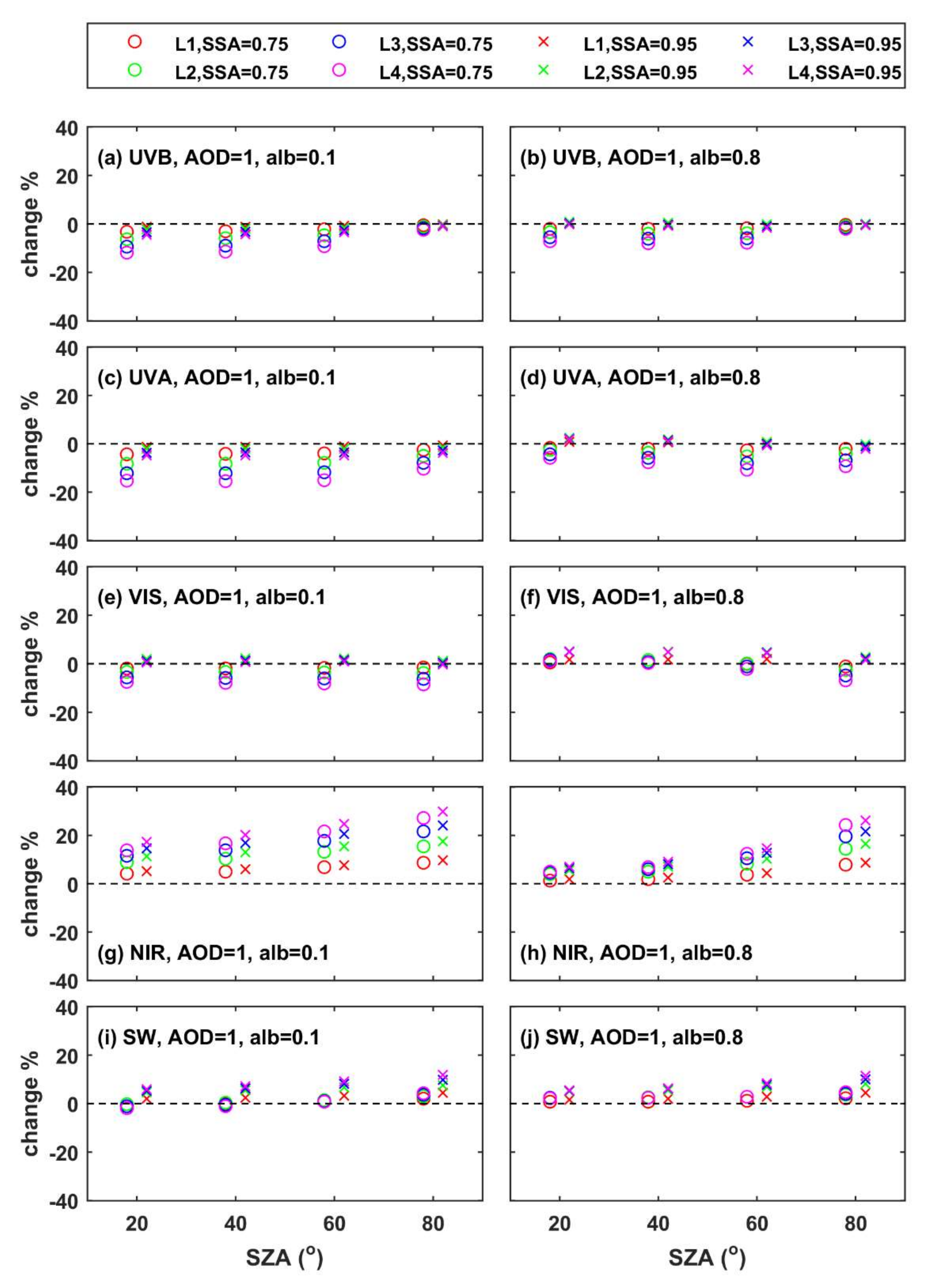
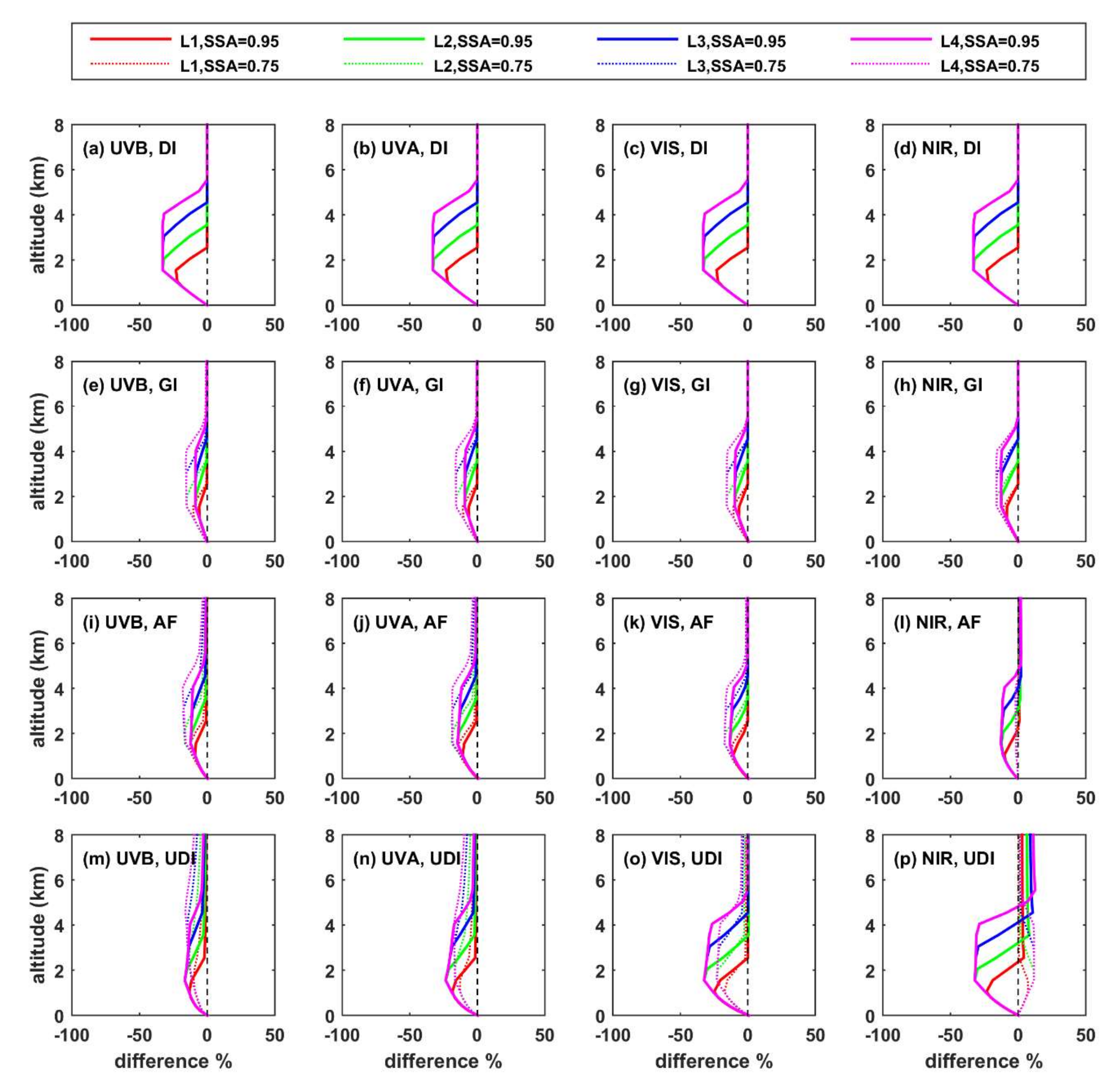
• The altitude of the aerosol layer has minor impact on the total shortwave GI at the BOA. Differences can be more significant for individual spectral regions, especially over high albedo surfaces, where increasing the altitude of the layer can lead to increases on the order of 10–15% in the UVB and UVA regions.
• For absorbing aerosols (SSA = 0.75), the SW UDI at the TOA practically does not change with changing altitude of the aerosol layer, while for more reflective aerosols (SSA = 0.95), the differences are larger, but again exceed 10% only at SZA = 80° and for large height differences in the altitude of the hypothetical aerosol layers.
• Increasing altitude of the aerosol layer corresponds to negative differences in the UDI in UVB, UVA, and VIS and positive differences in NIR at TOA. At BOA, the signs of differences in NIR are also opposite to the signs of changes in UVB, UVA, and VIS. This is because the changes in the fraction of photons that reach the BOA or the TOA are related with different processes in the different spectral regions. As also discussed in Mishra et al. [20], differences in the UV and VIS are mainly related with Rayleigh scattering, while differences in the NIR are mainly related with absorption in the atmosphere.
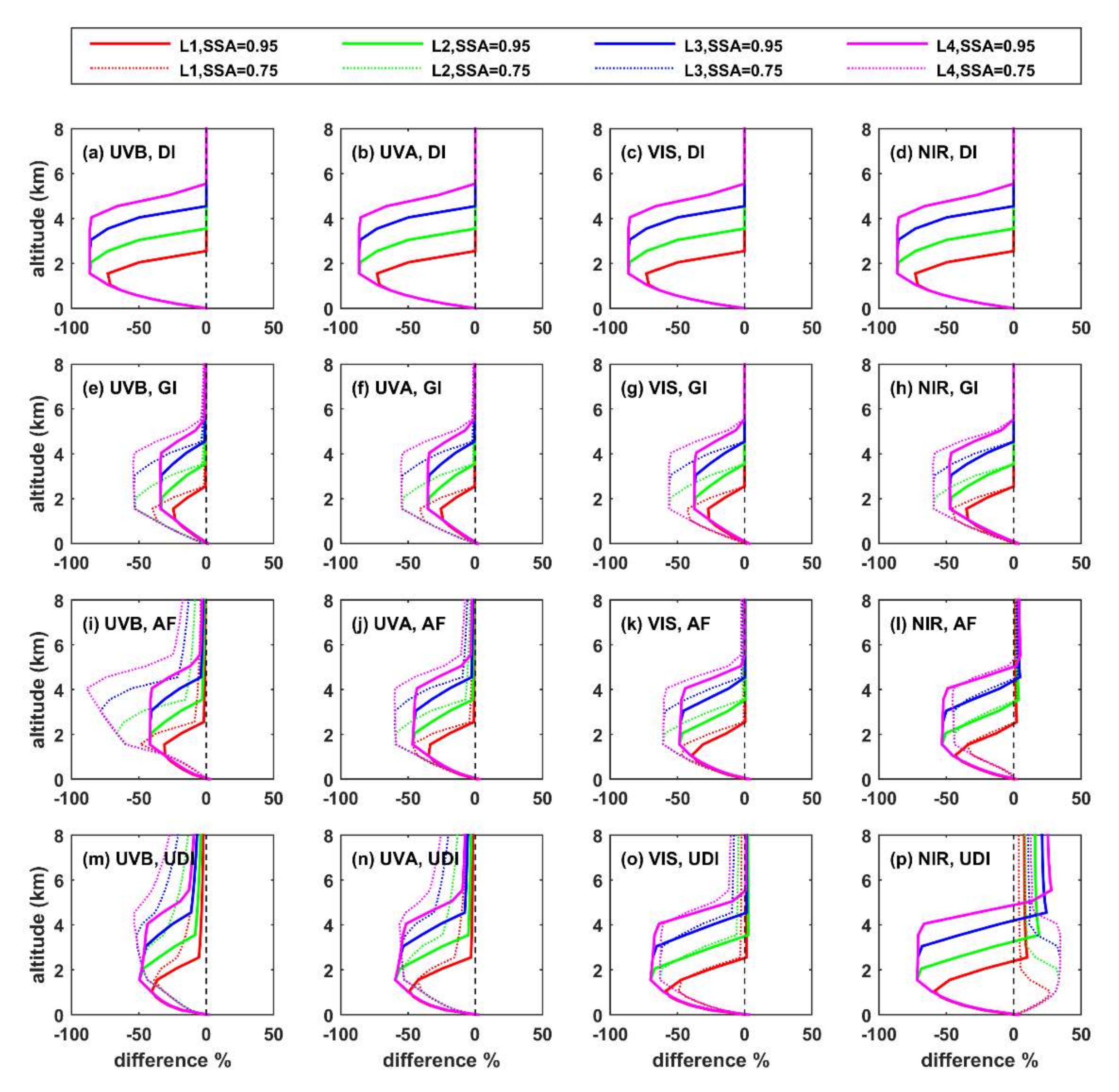
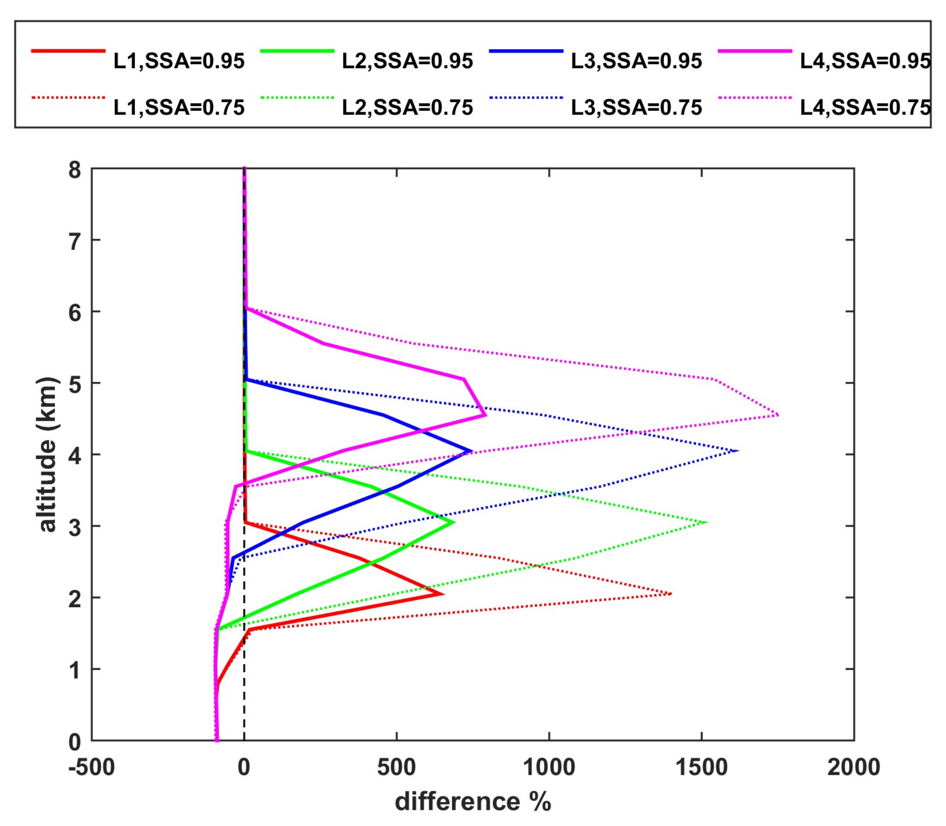
• Differences in the radiation profiles are larger in the atmosphere with respect to the TOA and the BOA. Increasing the altitude of the aerosol layer leads to a large increase in the SW HR at the level of the layer, and a large decrease at the level of L0, with respect to the case of having all aerosols at L0. Differences in AF are negative between the top of the elevated layer and the BOA when the AF profiles for elevated aerosol layers and aerosols at L0 are compared. For scattering aerosols (SSA = 0.95), differences in AF are more significant for longer (NIR) wavelengths, while for absorbing aerosols (SSA = 0.75), differences are more significant for shorter wavelengths (UVB). Increasing the SZA or the AOD increases the absolute differences, while increasing the surface albedo suppresses the differences.
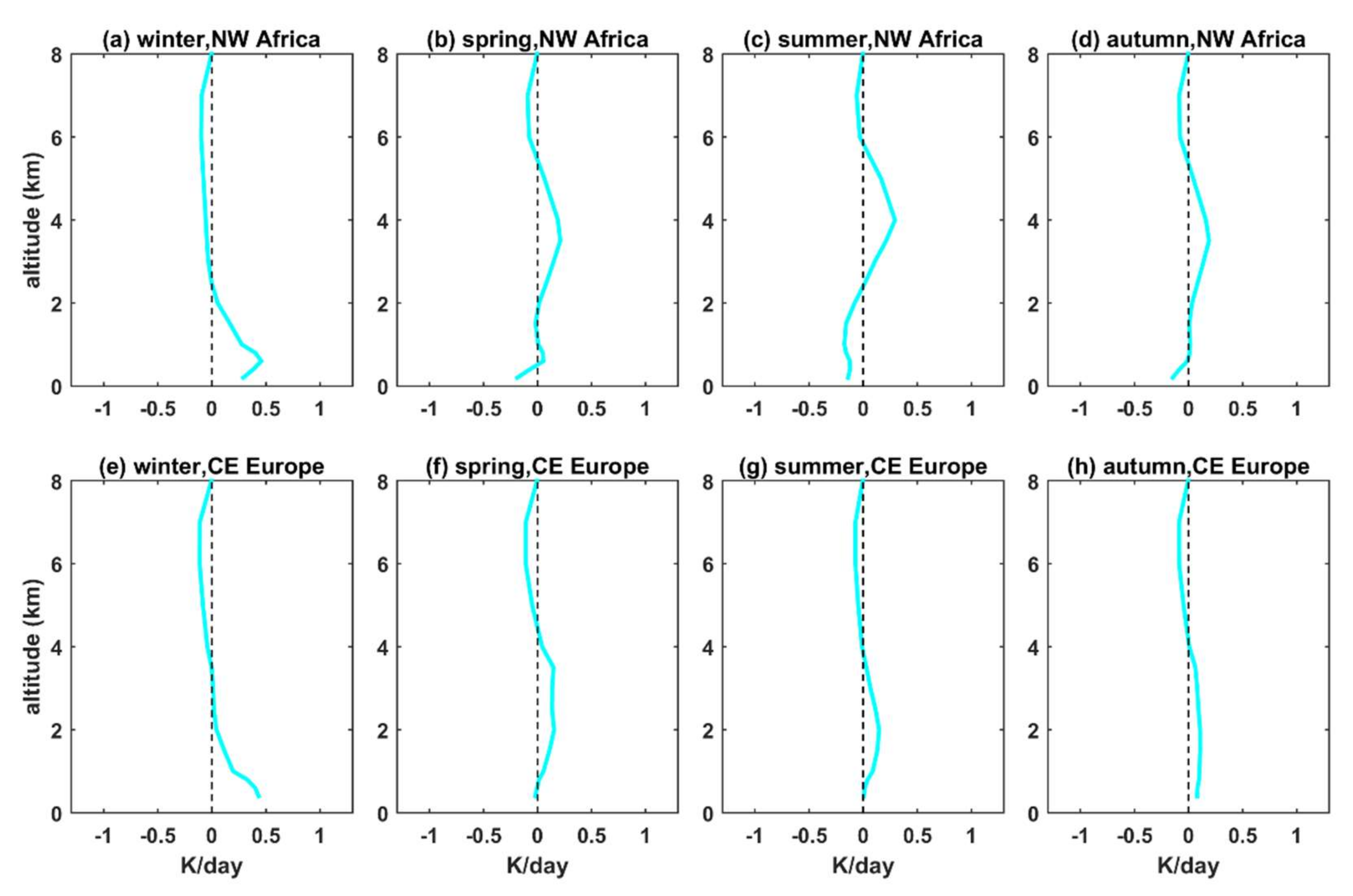
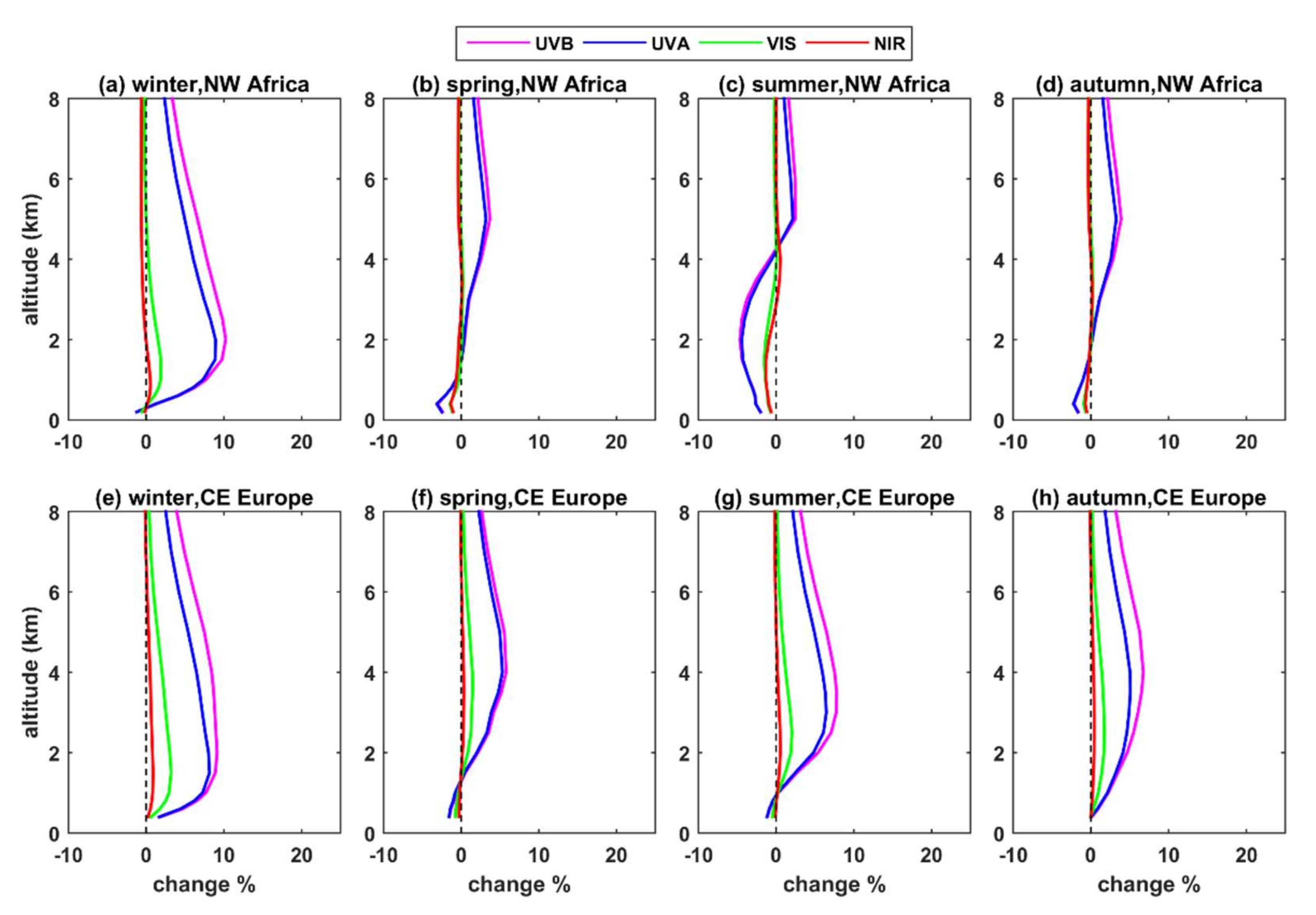
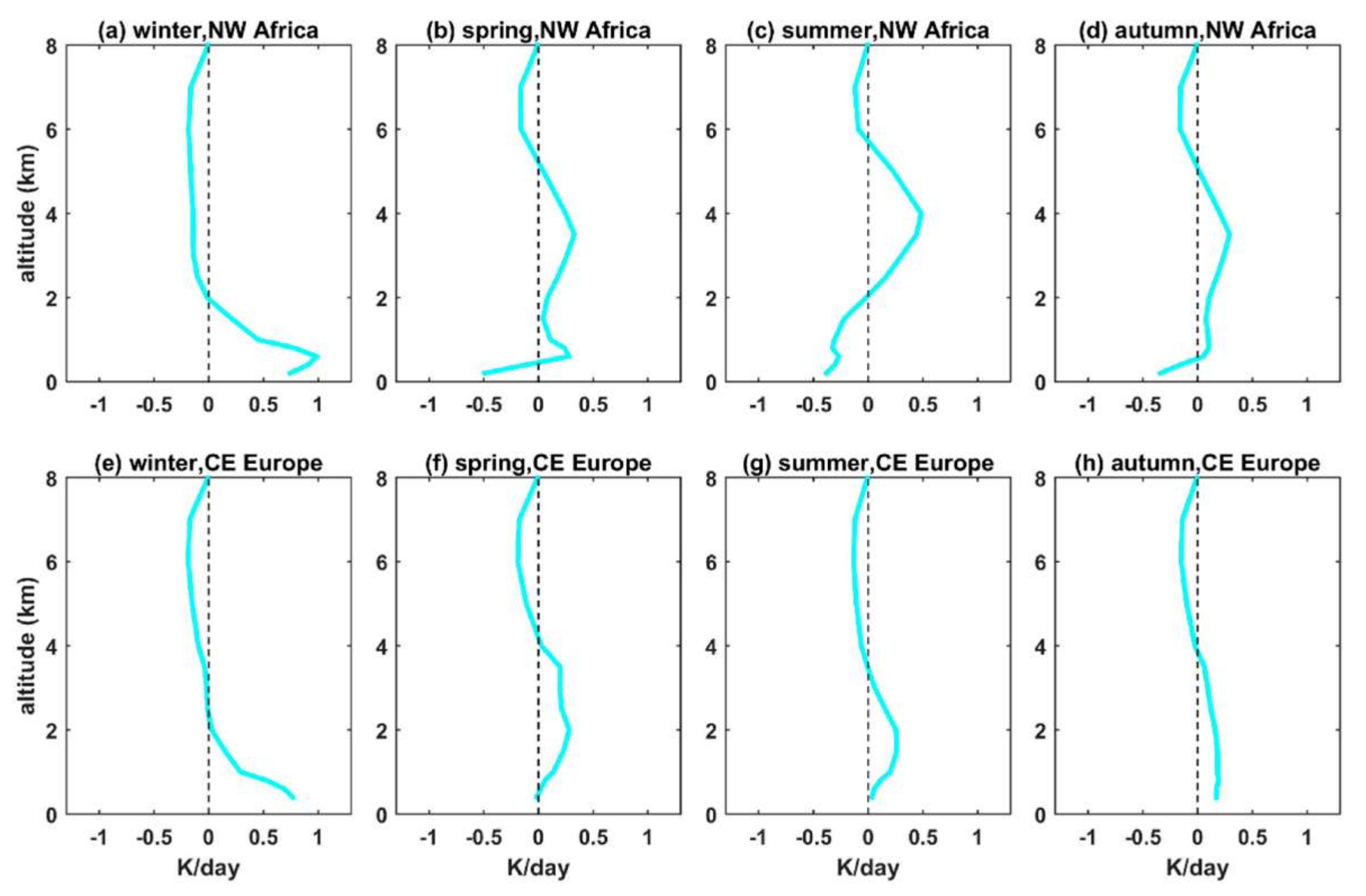
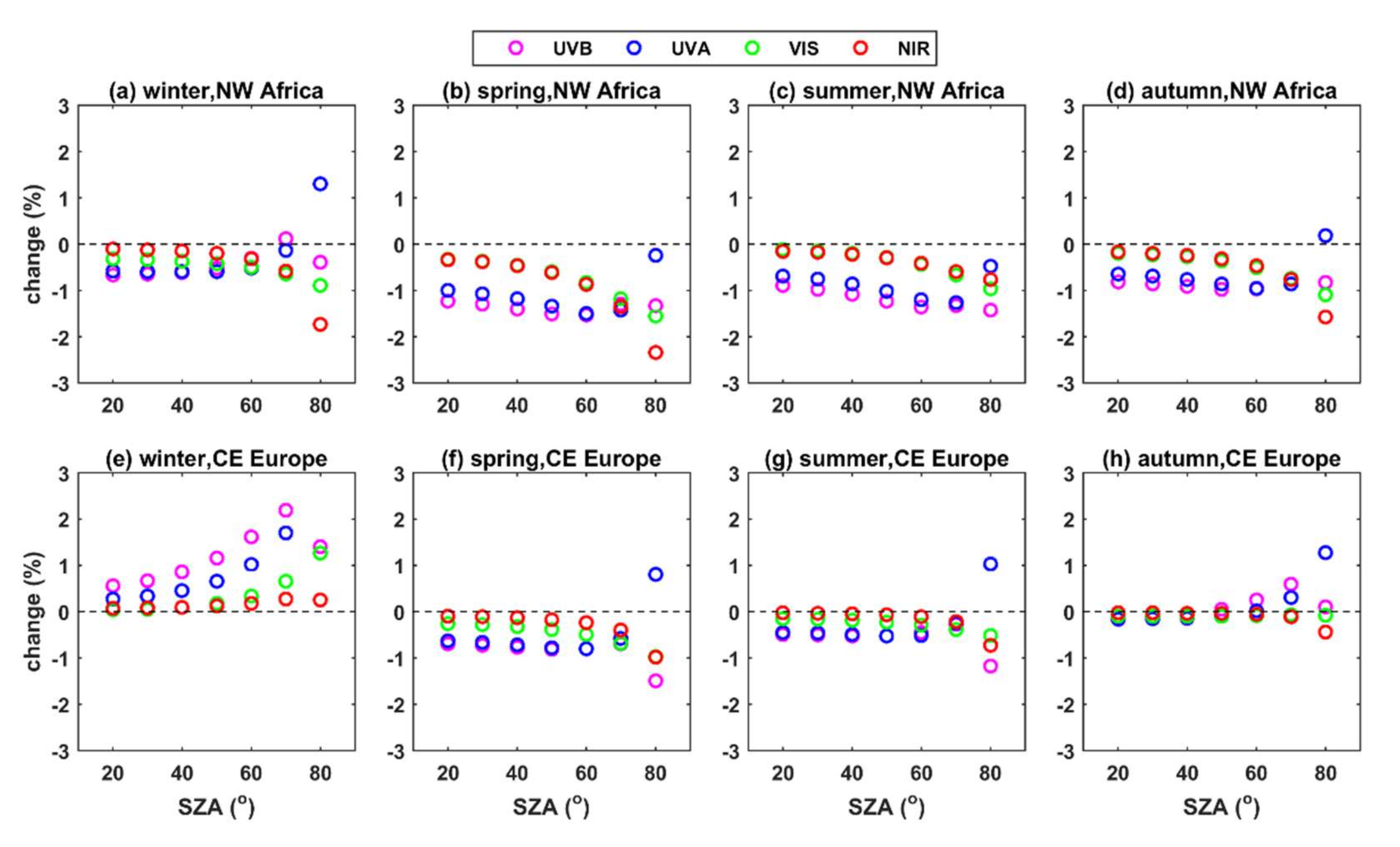
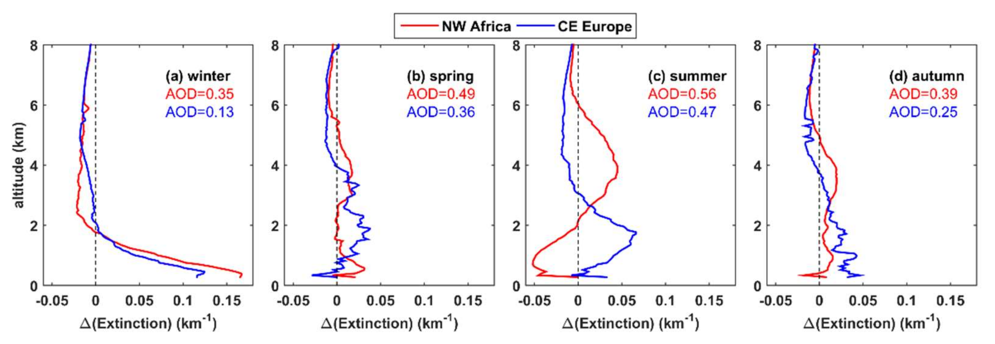
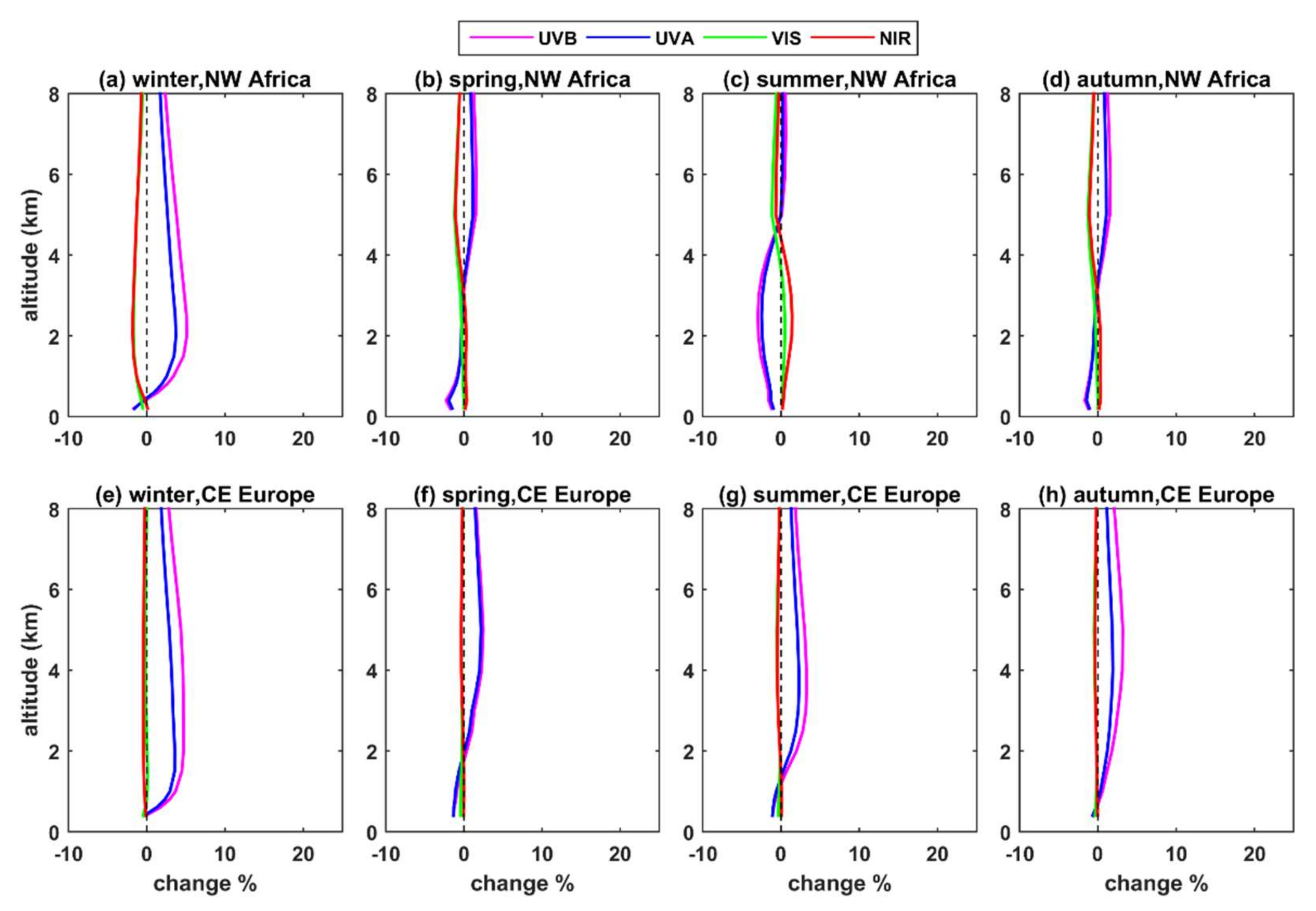
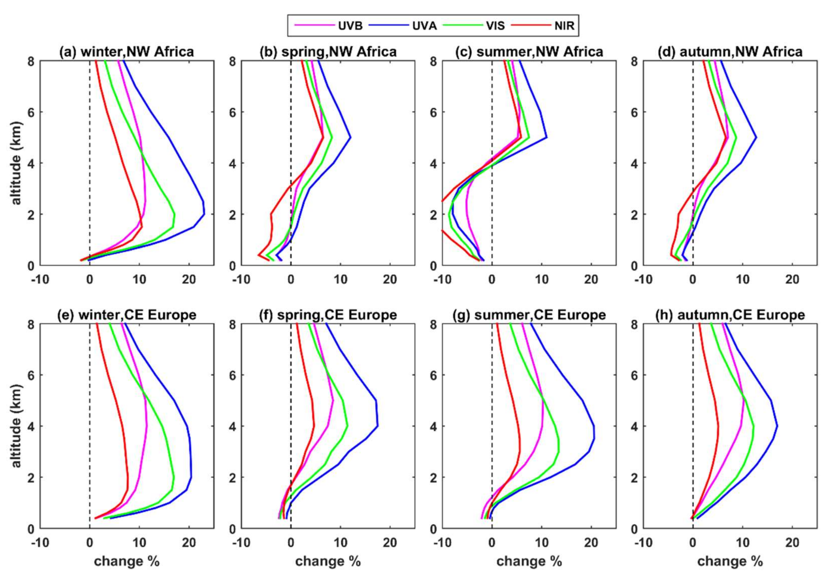
• For typical atmospheric and aerosol conditions in CE Europe and NW Africa, the differences in the UDI at the TOA and the GI at the BOA were, for all spectral bands (and obviously also for the SW radiation), below 5% when the seasonally averaged LIVAS profiles were used instead of the default profile. Differences in AF in the atmosphere were in most cases positive (i.e., more AF available for photochemical reactions when the LIVAS profiles were used), up to 10%, with the altitude of the maximum differences ranging between 1 km and 5 km depending on the region and the season. This was a consequence of the underestimation of the aerosol extinction by the default profile at low altitudes (near the surface). Differences in SW HR on the order of 0.5 to 1 K/day were found at the altitudes of maximum differences between the LIVAS and the default profile. Again, such differences cannot be considered negligible, since they can affect atmospheric stability, and subsequently the formation of clouds.
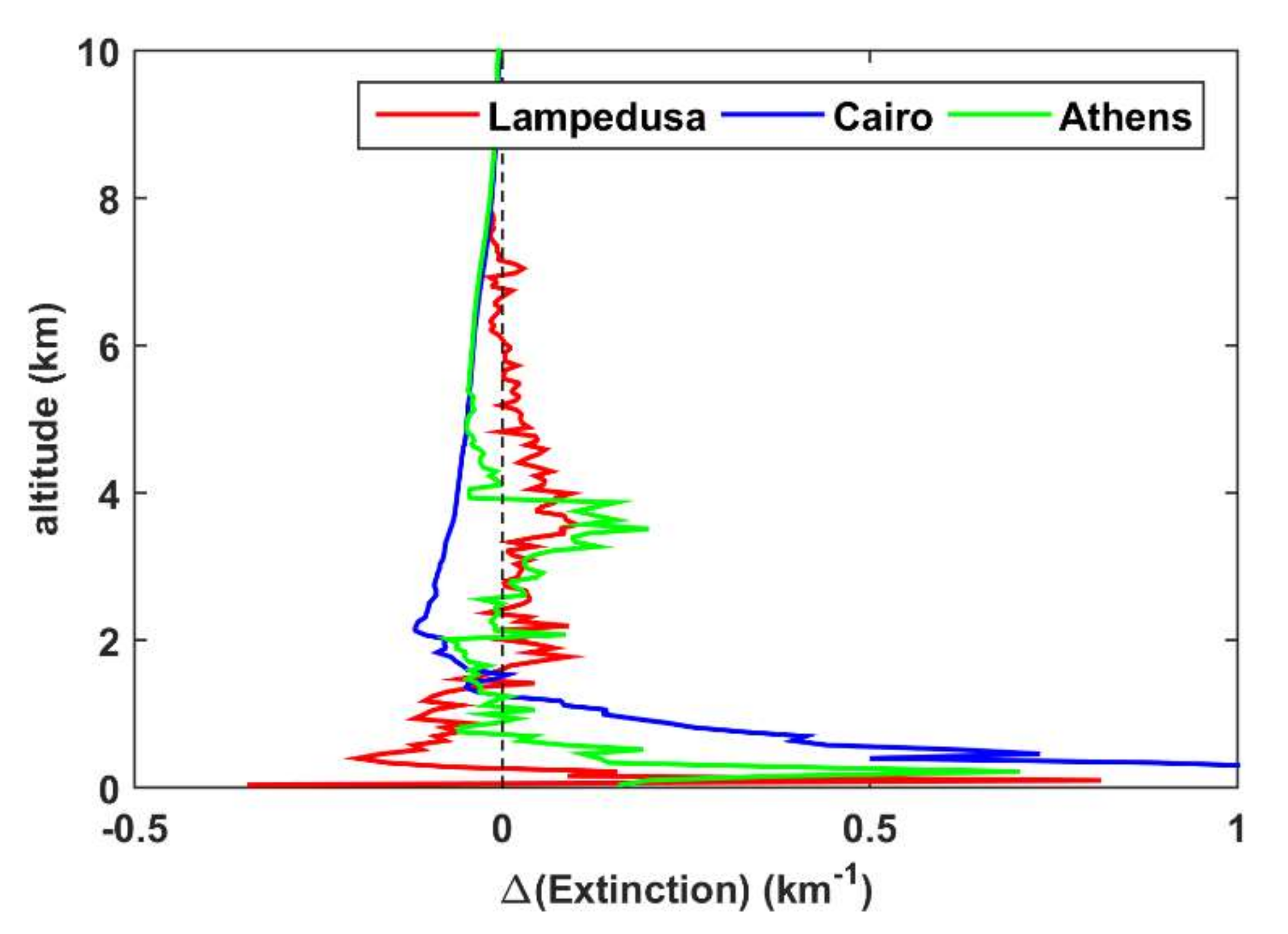
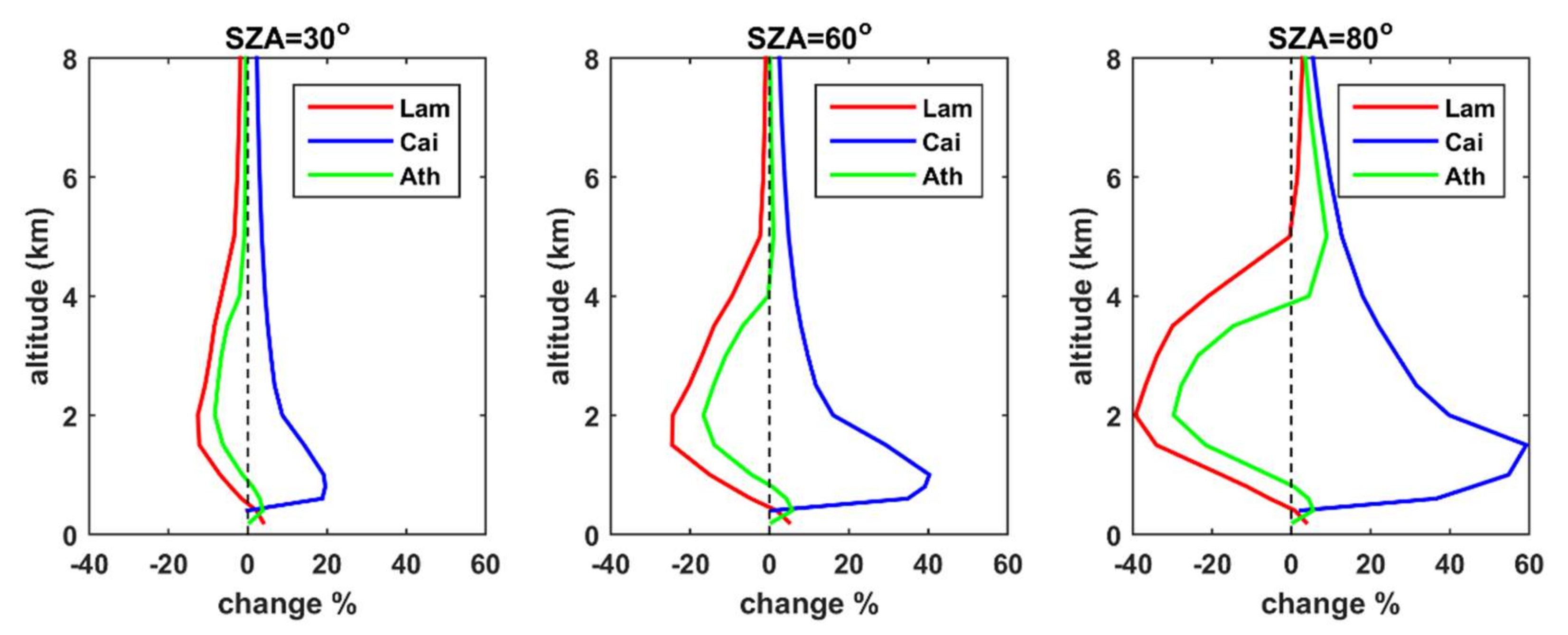
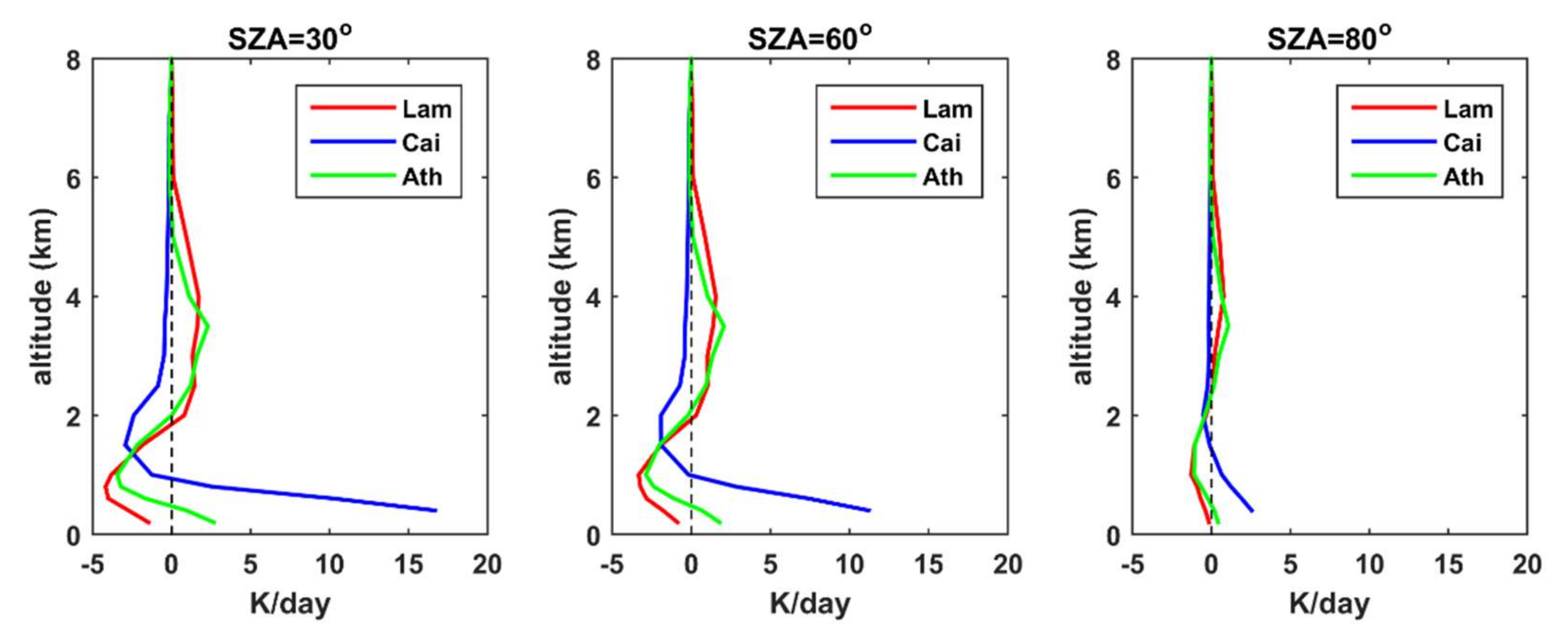
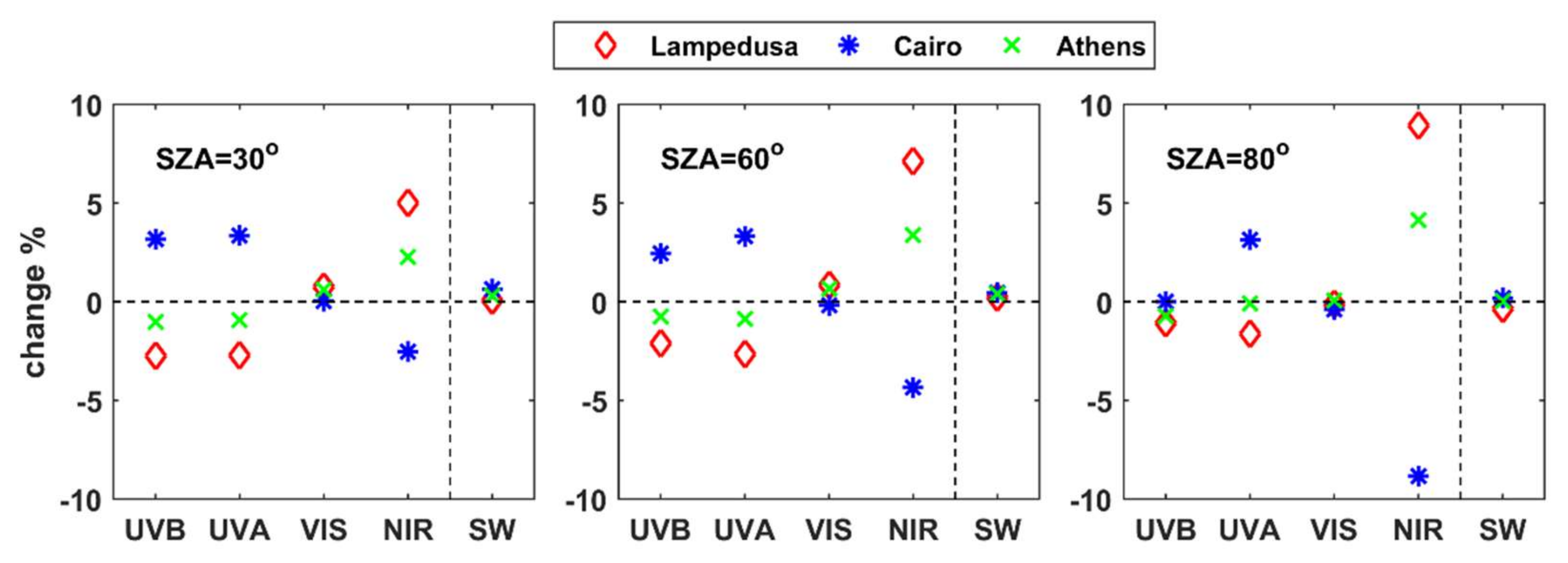
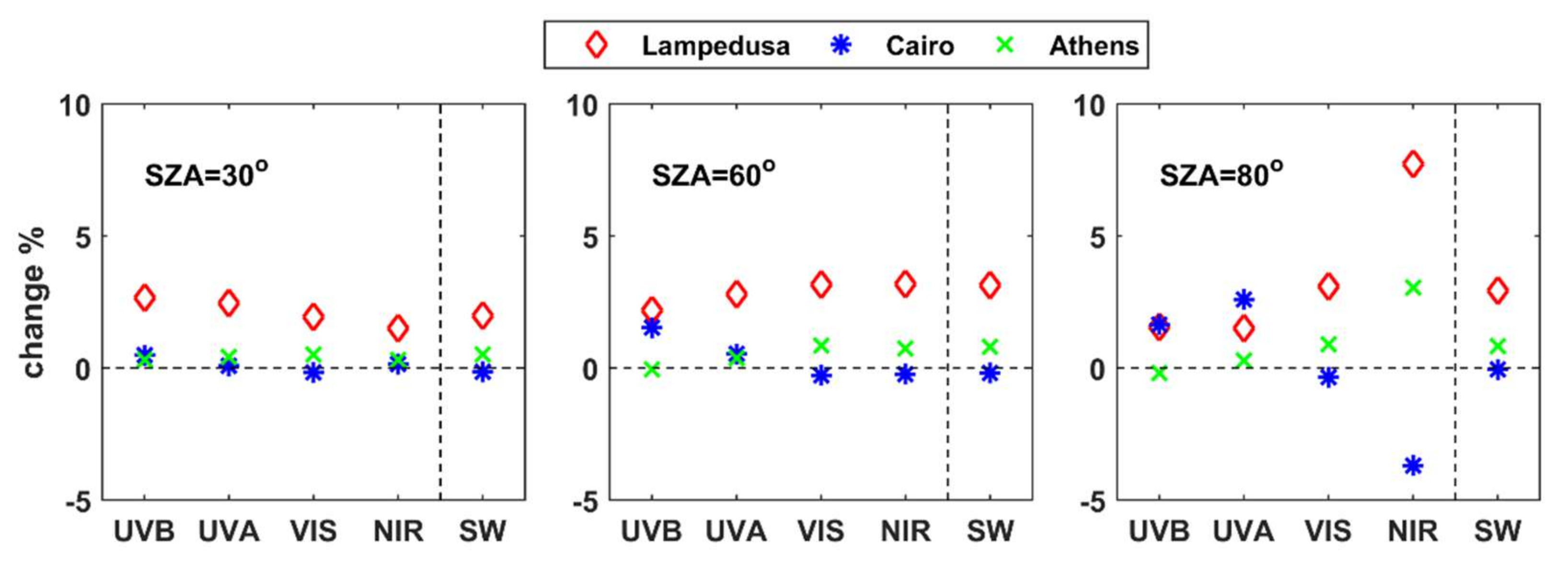
• At the three sites considered in the study, using average LIVAS instead of the theoretical extinction coefficient profiles for high AOD resulted in larger differences with respect to the comparison between the radiation profiles for average AOD conditions for the two regions. For Athens, the LIVAS extinction profile was closer to the theoretical, compared to the other two sites, resulting in the smallest differences in the radiation profile among the three sites. Differences in UV AF were negative at the lowest 4 km for Athens and Lampedusa, reaching −20% and −40% respectively at ~2 km when SZA = 80°. At the same SZA, differences in Cairo were positive, up to 60% at ~1.5 km. Differences in SW HR were also very large near the surface, reaching 17 K/day over Cairo for SZA = 30°. However, even for such a high aerosol load, differences at the BOA and the TOA were small, especially for the total SW radiation. Differences in SW UDI at the TOA were nearly zero for all sites, while differences in SW GI were smaller than 3% at BOA. Differences in individual spectral bands were more significant, mainly for NIR at high SZAs, where they could be on the order of 10% at TOA and 5–8% at the BOA.

As already discussed, using a more realistic extinction coefficient profile for the simulations of the vertical profile of the SW radiation leads to small differences at the BOA and the TOA for typical AOD conditions. Thus, using measured profiles for climatological studies of the radiative effects of aerosols is not critical. This is in agreement with the findings of Petrzala et al. for urban aerosols [23]. According to Mishra et al. [20], differences can be more significant for the thermal infrared (4–20 μm) spectral region (longwave radiation). The role of the aerosol profile also can be more significant in the presence of clouds (e.g., [78]). The present study was, however, focused on radiative effects in different bands of SW solar radiation under cloudless-sky conditions.

Even if the results of the present study confirm that accurately determined AOD plays the most significant role in RT simulations of aerosol radiation interactions, aerosol profile retrievals from lidar instruments and satellite observations (e.g., CALIPSO [57] and the upcoming Cloud, Aerosol and Radiation Explorer—EarthCARE mission [79]) could be used to improve such simulations. For individual spectral bands (UV or NIR), using a more realistic profile was found to increase the accuracy in aerosol radiative effect-related studies involving elevated aerosol layers and high AOD (e.g., dust or smoke events), even under cloudless skies, especially over high-albedo terrains. Changes in the vertical distribution of aerosols were found to have a very significant impact on the HR and AF, even for low aerosol loads. Photochemical reactions at altitudes of up to 3 km may affect the composition and quality of air inside the boundary layer. Thus, differences in the vertical distribution of AF, especially in the UV, lead to changes in the atmospheric photochemistry and subsequently the atmospheric composition [80,81]. Large differences in HR can significantly affect atmospheric processes such as the formation of clouds [82] or the formation of the PBL [83]. Very large differences in HR and AF were found during dust events over Mediterranean sites, denoting correspondingly large uncertainties in the modeling of atmospheric and photochemical processes if the aerosol vertical distribution is not accurately taken into account.

The findings of the study already highlight the significant role of aerosols regarding the distribution of solar radiation in the atmosphere, and shows that improved descriptions of the aerosol extinction coefficient profiles in numerical, regional and global models would lead to improved descriptions of chemical and physical processes that take place in the atmosphere, and subsequently to improved products for studies of air quality and climate.

In conclusion, the present study aimed to contribute towards the understanding of the role of the vertical distribution of aerosols in the modeling of the transfer of solar radiation in the atmosphere, and to set the basis for further and deeper investigations under more complex conditions and with respect to other atmospheric processes. Extension of the present study could include simulations of the longwave radiation and interactions with clouds. Investigation of the effects of the vertical distribution of more aerosol properties (SSA, asymmetry parameter, etc.) would also lead to a deeper understanding of the role of aerosols in the atmosphere.

References

1. Wild, M. Global dimming and brightening: A review. J. Geophys. Res. Atmos. 2009, 114. [Google Scholar] [CrossRef] [Green Version]
2. Wild, M. Decadal changes in radiative fluxes at land and ocean surfaces and their relevance for global warming. WIREs Clim. Change 2016, 7, 91–107. [Google Scholar] [CrossRef]
3. Wild, M.; Folini, D.; Henschel, F.; Fischer, N.; Müller, B. Projections of long-term changes in solar radiation based on CMIP5 climate models and their influence on energy yields of photovoltaic systems. Sol. Energy 2015, 116, 12–24. [Google Scholar] [CrossRef] [Green Version]
4. Stocker, T.F.; Qin, D.; Plattner, G.K.; Tignor, M.M.; Allen, S.K.; Boschung, J.; Nauels, A.; Xia, Y.; Bex, V.; Midgley, P.M. (Eds.) Climate Change 2013: The Physical Science Basis. Contribution of Working Group I to the Fifth Assessment Report of the Intergovernmental Panel on Climate Change; Cambridge University Press: New York, NY, USA, 2013. [Google Scholar]
5. Otto, S.; Bierwirth, E.; Weinzierl, B.; Kandler, K.; Esselborn, M.; Tesche, M.; Schladitz, A.; Wendisch, M.; Trautmann, T. Solar radiative effects of a Saharan dust plume observed during SAMUM assuming spheroidal model particles. Tellus B Chem. Phys. Meteorol. 2009, 61, 270–296. [Google Scholar] [CrossRef] [Green Version]
6. Otto, S.; de Reus, M.; Trautmann, T.; Thomas, A.; Wendisch, M.; Borrmann, S. Atmospheric radiative effects of an in situ measured Saharan dust plume and the role of large particles. Atmos. Chem. Phys. 2007, 7, 4887–4903. [Google Scholar] [CrossRef] [Green Version]
7. Zeng, L.; Zhang, A.; Wang, Y.; Wagner, N.L.; Katich, J.M.; Schwarz, J.P.; Schill, G.P.; Brock, C.; Froyd, K.D.; Murphy, D.M.; et al. Global measurements of brown carbon and estimated direct radiative effects. Geophys. Res. Lett. 2020, 47, e2020GL088747. [Google Scholar] [CrossRef]
8. Hess, M.; Koepke, P.; Schult, I. Optical properties of aerosols and clouds: The software package OPAC. Bull. Am. Meteorol. Soc. 1998, 79, 831–844. [Google Scholar] [CrossRef]
9. Tsekeri, A.; Lopatin, A.; Amiridis, V.; Marinou, E.; Igloffstein, J.; Siomos, N.; Solomos, S.; Kokkalis, P.; Engelmann, R.; Baars, H.; et al. GARRLiC and LIRIC: Strengths and limitations for the characterization of dust and marine particles along with their mixtures. Atmos. Meas. Tech. 2017, 10, 4995–5016. [Google Scholar] [CrossRef] [Green Version]
10. Chen, L. Uncertainties in solar radiation assessment in the United States using climate models. Clim. Dyn. 2021, 56, 665–678. [Google Scholar] [CrossRef]
11. Boé, J.; Somot, S.; Corre, L.; Nabat, P. Large discrepancies in summer climate change over Europe as projected by global and regional climate models: Causes and consequences. Clim. Dyn. 2020, 54, 2981–3002. [Google Scholar] [CrossRef]
12. Bartók, B.; Wild, M.; Folini, D.; Lüthi, D.; Kotlarski, S.; Schär, C.; Vautard, R.; Jerez, S.; Imecs, Z. Projected changes in surface solar radiation in CMIP5 global climate models and in EURO-CORDEX regional climate models for Europe. Clim. Dyn. 2017, 49, 2665–2683. [Google Scholar] [CrossRef]
13. Lakkala, K.; Kujanpää, J.; Brogniez, C.; Henriot, N.; Arola, A.; Aun, M.; Auriol, F.; Bais, A.F.; Bernhard, G.; de Bock, V.; et al. Validation of the TROPOspheric Monitoring Instrument (TROPOMI) surface UV radiation product. Atmos. Meas. Tech. 2020, 13, 6999–7024. [Google Scholar] [CrossRef]
14. Zempila, M.M.; Fountoulakis, I.; Taylor, M.; Kazadzis, S.; Arola, A.; Koukouli, M.E.; Bais, A.; Meleti, C.; Balis, D. Validation of OMI erythemal doses with multi-sensor ground-based measurements in Thessaloniki, Greece. Atmos. Environ. 2018, 183, 106–121. [Google Scholar] [CrossRef] [Green Version]
15. Merrouni, A.A.; Ghennioui, A.; Wolfertstetter, F.; Mezrhab, A. The uncertainty of the HelioClim-3 DNI data under Moroccan climate. AIP Conf. Proc. 2017, 1850, 140002. [Google Scholar] [CrossRef] [Green Version]
16. Witthuhn, J.; Hünerbein, A.; Filipitsch, F.; Wacker, S.; Meilinger, S.; Deneke, H. Aerosol properties and aerosol–radiation interactions in clear-sky conditions over Germany. Atmos. Chem. Phys. 2021, 21, 14591–14630. [Google Scholar] [CrossRef]
17. Raptis, I.-P.; Kazadzis, S.; Eleftheratos, K.; Amiridis, V.; Fountoulakis, I. Single scattering albedo’s spectral dependence effect on UV irradiance. Atmosphere 2018, 9, 364. [Google Scholar] [CrossRef] [Green Version]
18. Bergstrom, R.W.; Pilewskie, P.; Russell, P.B.; Redemann, J.; Bond, T.C.; Quinn, P.K.; Sierau, B. Spectral absorption properties of atmospheric aerosols. Atmos. Chem. Phys. 2007, 7, 5937–5943. [Google Scholar] [CrossRef] [Green Version]
19. Fountoulakis, I.; Natsis, A.; Siomos, N.; Drosoglou, T.; Bais, A.F. Deriving aerosol absorption properties from solar ultraviolet radiation spectral measurements at Thessaloniki, Greece. Remote Sens. 2019, 11, 2179. [Google Scholar] [CrossRef] [Green Version]
20. Mishra, A.K.; Koren, I.; Rudich, Y. Effect of aerosol vertical distribution on aerosol-radiation interaction: A theoretical prospect. Heliyon 2015, 1, e00036. [Google Scholar] [CrossRef] [Green Version]
21. Stevens, B.; Fiedler, S.; Kinne, S.; Peters, K.; Rast, S.; Müsse, J.; Smith, S.J.; Mauritsen, T. MACv2-SP: A parameterization of anthropogenic aerosol optical properties and an associated Twomey effect for use in CMIP6. Geosci. Model Dev. 2017, 10, 433–452. [Google Scholar] [CrossRef] [Green Version]
22. Shettle, E. Models of aerosols, clouds, and precipitation for atmospheric propagation studies. AGARD Conf. Proc. 1989. Available online: https://www.researchgate.net/publication/234312286_Models_of_aerosols_clouds_and_precipitation_for_atmospheric_propagation_studies (accessed on 15 January 2021).
23. Petrzala, J. Assessment of influence of urban aerosol vertical profile on clear-sky diffuse radiance pattern. J. Sol. Energy Eng. 2021, 144, 1–7. [Google Scholar] [CrossRef]
24. Marinou, E.; Amiridis, V.; Binietoglou, I.; Tsikerdekis, A.; Solomos, S.; Proestakis, E.; Konsta, D.; Papagiannopoulos, N.; Tsekeri, A.; Vlastou, G.; et al. Three-dimensional evolution of Saharan dust transport towards Europe based on a 9-year EARLINET-optimized CALIPSO dataset. Atmos. Chem. Phys. 2017, 17, 5893–5919. [Google Scholar] [CrossRef] [Green Version]
25. Langmann, B.; Folch, A.; Hensch, M.; Matthias, V. Volcanic ash over Europe during the eruption of Eyjafjallajökull on Iceland, April–May 2010. Atmos. Environ. 2012, 48, 1–8. [Google Scholar] [CrossRef]
26. Bernard, A.; Rose, W.I. The injection of sulfuric acid aerosols in the stratosphere by the El Chichón volcano and its related hazards to the international air traffic. Nat. Hazards 1990, 3, 59–67. [Google Scholar] [CrossRef]
27. Osborne, M.; Malavelle, F.F.; Adam, M.; Buxmann, J.; Sugier, J.; Marenco, F.; Haywood, J. Saharan dust and biomass burning aerosols during ex-hurricane Ophelia: Observations from the new UK lidar and sun-photometer network. Atmos. Chem. Phys. 2019, 19, 3557–3578. [Google Scholar] [CrossRef] [Green Version]
28. Vaughan, G.; Wareing, D.; Ricketts, H. Measurement report: Lidar measurements of stratospheric aerosol following the 2019 Raikoke and Ulawun volcanic eruptions. Atmos. Chem. Phys. 2021, 21, 5597–5604. [Google Scholar] [CrossRef]
29. Labonne, M.; Bréon, F.-M.; Chevallier, F. Injection height of biomass burning aerosols as seen from a spaceborne lidar. Geophys. Res. Lett. 2007, 34. [Google Scholar] [CrossRef]
30. Garratt, J.R. Review: The atmospheric boundary layer. Earth-Sci. Rev. 1994, 37, 89–134. [Google Scholar] [CrossRef]
31. Soupiona, O.; Papayannis, A.; Kokkalis, P.; Foskinis, R.; Sánchez Hernández, G.; Ortiz-Amezcua, P.; Mylonaki, M.; Papanikolaou, C.-A.; Papagiannopoulos, N.; Samaras, S.; et al. EARLINET observations of Saharan dust intrusions over the northern Mediterranean region (2014–2017): Properties and impact on radiative forcing. Atmos. Chem. Phys. 2020, 20, 15147–15166. [Google Scholar] [CrossRef]
32. Herut, B.; Rahav, E.; Tsagaraki, T.M.; Giannakourou, A.; Tsiola, A.; Psarra, S.; Lagaria, A.; Papageorgiou, N.; Mihalopoulos, N.; Theodosi, C.N.; et al. The potential impact of saharan dust and polluted aerosols on microbial populations in the east Mediterranean Sea, an overview of a mesocosm experimental approach. Front. Mar. Sci. 2016, 3, 226. [Google Scholar] [CrossRef] [Green Version]
33. Fountoulakis, I.; Kosmopoulos, P.; Papachristopoulou, K.; Raptis, I.-P.; Mamouri, R.-E.; Nisantzi, A.; Gkikas, A.; Witthuhn, J.; Bley, S.; Moustaka, A.; et al. Effects of aerosols and clouds on the levels of surface solar radiation and solar energy in Cyprus. Remote Sens. 2021, 13, 2319. [Google Scholar] [CrossRef]
34. Kosmopoulos, P.G.; Kazadzis, S.; El-Askary, H.; Taylor, M.; Gkikas, A.; Proestakis, E.; Kontoes, C.; El-Khayat, M.M. Earth-observation-based estimation and forecasting of particulate matter impact on solar energy in Egypt. Remote Sens. 2018, 10, 1870. [Google Scholar] [CrossRef] [Green Version]
35. Rizza, U.; Canepa, E.; Ricchi, A.; Bonaldo, D.; Carniel, S.; Morichetti, M.; Passerini, G.; Santiloni, L.; Scremin Puhales, F.; Miglietta, M.M. Influence of wave state and sea spray on the roughness length: Feedback on medicanes. Atmosphere 2018, 9, 301. [Google Scholar] [CrossRef] [Green Version]
36. Varlas, G.; Marinou, E.; Gialitaki, A.; Siomos, N.; Tsarpalis, K.; Kalivitis, N.; Solomos, S.; Tsekeri, A.; Spyrou, C.; Tsichla, M.; et al. Assessing sea-state effects on sea-salt aerosol modeling in the lower atmosphere using lidar and in-situ measurements. Remote Sens. 2021, 13, 614. [Google Scholar] [CrossRef]
37. Revell, L.E.; Kuma, P.; le Ru, E.C.; Somerville, W.R.C.; Gaw, S. Direct radiative effects of airborne microplastics. Nature 2021, 598, 462–467. [Google Scholar] [CrossRef] [PubMed]
38. Trainic, M.; Flores, J.M.; Pinkas, I.; Pedrotti, M.L.; Lombard, F.; Bourdin, G.; Gorsky, G.; Boss, E.; Rudich, Y.; Vardi, A.; et al. Airborne microplastic particles detected in the remote marine atmosphere. Commun. Earth Environ. 2020, 1, 64. [Google Scholar] [CrossRef]
39. Allen, S.; Allen, D.; Baladima, F.; Phoenix, V.R.; Thomas, J.L.; le Roux, G.; Sonke, J.E. Evidence of free tropospheric and long-range transport of microplastic at Pic du Midi Observatory. Nat. Commun. 2021, 12, 7242. [Google Scholar] [CrossRef]
40. Fasano, G.; Diémoz, H.; Fountoulakis, I.; Cassardo, C.; Kudo, R.; Siani, A.M.; Ferrero, L. Vertical profile of the clear-sky aerosol direct radiative effect in an Alpine valley, by the synergy of ground-based measurements and radiative transfer simulations. Bull. Atmos. Sci. Technol. 2021, 2, 11. [Google Scholar] [CrossRef]
41. Thornton, J.M.; Palazzi, E.; Pepin, N.C.; Cristofanelli, P.; Essery, R.; Kotlarski, S.; Giuliani, G.; Guigoz, Y.; Kulonen, A.; Pritchard, D.; et al. Toward a definition of Essential Mountain Climate Variables. One Earth 2021, 4, 805–827. [Google Scholar] [CrossRef]
42. Pepin, N.; Bradley, R.S.; Diaz, H.F.; Baraer, M.; Caceres, E.B.; Forsythe, N.; Fowler, H.; Greenwood, G.; Hashmi, M.Z.; Liu, X.D.; et al. Elevation-dependent warming in mountain regions of the world. Nat. Clim. Change 2015, 5, 424–430. [Google Scholar] [CrossRef] [Green Version]
43. Lau, K.M.; Kim, M.K.; Kim, K.M. Asian summer monsoon anomalies induced by aerosol direct forcing: The role of the Tibetan Plateau. Clim. Dyn. 2006, 26, 855–864. [Google Scholar] [CrossRef] [Green Version]
44. Surabi, M.; James, H.; Larissa, N.; Yunfeng, L. Climate effects of black carbon aerosols in China and India. Science 2002, 297, 2250–2253. [Google Scholar] [CrossRef] [Green Version]
45. Lau, K.-M.; Kim, K.-M. Observational relationships between aerosol and Asian monsoon rainfall, and circulation. Geophys. Res. Lett. 2006, 33. [Google Scholar] [CrossRef]
46. Crutzen, P.J.; Zimmermann, P.H. The changing photochemistry of the troposphere. Tellus B Chem. Phys. Meteorol. 1991, 43, 136–151. [Google Scholar] [CrossRef]
47. Carroll, M.A.; Ridley, B.A.; Montzka, D.D.; Hubler, G.; Walega, J.G.; Norton, R.B.; Huebert, B.J.; Grahek, F.E. Measurements of nitric oxide and nitrogen dioxide during the Mauna Loa Observatory Photochemistry Experiment. J. Geophys. Res. Atmos. 1992, 97, 10361–10374. [Google Scholar] [CrossRef]
48. Topaloglou, C.; Kazadzis, S.; Bais, A.F.; Blumthaler, M.; Schallhart, B.; Balis, D. NO2 and HCHO photolysis frequencies from irradiance measurements in Thessaloniki, Greece. Atmos. Chem. Phys. 2005, 5, 1645–1653. [Google Scholar] [CrossRef] [Green Version]
49. Zhang, Y.; Xue, L.; Dong, C.; Wang, T.; Mellouki, A.; Zhang, Q.; Wang, W. Gaseous carbonyls in China’s atmosphere: Tempo-spatial distributions, sources, photochemical formation, and impact on air quality. Atmos. Environ. 2019, 214, 116863. [Google Scholar] [CrossRef]
50. Edinger, J.G. Vertical distribution of photochemical smog in Los Angeles basin. Environ. Sci. Technol. 1973, 7, 247–252. [Google Scholar] [CrossRef]
51. Velasco, E.; Márquez, C.; Bueno, E.; Bernabé, R.M.; Sánchez, A.; Fentanes, O.; Wöhrnschimmel, H.; Cárdenas, B.; Kamilla, A.; Wakamatsu, S.; et al. Vertical distribution of ozone and VOCs in the low boundary layer of Mexico City. Atmos. Chem. Phys. 2008, 8, 3061–3079. [Google Scholar] [CrossRef] [Green Version]
52. Diémoz, H.; Barnaba, F.; Magri, T.; Pession, G.; Dionisi, D.; Pittavino, S.; Tombolato, I.K.F.; Campanelli, M.; Della Ceca, L.S.; Hervo, M.; et al. Transport of Po Valley aerosol pollution to the northwestern Alps—Part 1: Phenomenology. Atmos. Chem. Phys. 2019, 19, 3065–3095. [Google Scholar] [CrossRef] [Green Version]
53. Liao, H.; Yung, Y.L.; Seinfeld, J.H. Effects of aerosols on tropospheric photolysis rates in clear and cloudy atmospheres. J. Geophys. Res. Atmos. 1999, 104, 23697–23707. [Google Scholar] [CrossRef] [Green Version]
54. Wang, W.; Li, X.; Shao, M.; Hu, M.; Zeng, L.; Wu, Y.; Tan, T. The impact of aerosols on photolysis frequencies and ozone production in Beijing during the 4-year period 2012–2015. Atmos. Chem. Phys. 2019, 19, 9413–9429. [Google Scholar] [CrossRef] [Green Version]
55. Kylling, A.; Webb, A.R.; Kift, R.; Gobbi, G.P.; Ammannato, L.; Barnaba, F.; Bais, A.; Kazadzis, S.; Wendisch, M.; Jäkel, E.; et al. Spectral actinic flux in the lower troposphere: Measurement and 1-D simulations for cloudless, broken cloud and overcast situations. Atmos. Chem. Phys. 2005, 5, 1975–1997. [Google Scholar] [CrossRef] [Green Version]
56. Amiridis, V.; Marinou, E.; Tsekeri, A.; Wandinger, U.; Schwarz, A.; Giannakaki, E.; Mamouri, R.; Kokkalis, P.; Binietoglou, I.; Solomos, S.; et al. LIVAS: A 3-D multi-wavelength aerosol/cloud database based on CALIPSO and EARLINET. Atmos. Chem. Phys. 2015, 15, 7127–7153. [Google Scholar] [CrossRef] [Green Version]
57. Winker, D.M.; Pelon, J.; Coakley, J.A.; Ackerman, S.A.; Charlson, R.J.; Colarco, P.R.; Flamant, P.; Fu, Q.; Hoff, R.M.; Kittaka, C.; et al. The CALIPSO mission: A global 3D view of aerosols and clouds. Bull. Am. Meteorol. Soc. 2010, 91, 1211–1230. [Google Scholar] [CrossRef]
58. Gkikas, A.; Proestakis, E.; Amiridis, V.; Kazadzis, S.; di Tomaso, E.; Tsekeri, A.; Marinou, E.; Hatzianastassiou, N.; Pérez García-Pando, C. ModIs Dust AeroSol (MIDAS): A global fine-resolution dust optical depth data set. Atmos. Meas. Tech. 2021, 14, 309–334. [Google Scholar] [CrossRef]
59. Proestakis, E.; Amiridis, V.; Marinou, E.; Georgoulias, A.K.; Solomos, S.; Kazadzis, S.; Chimot, J.; Che, H.; Alexandri, G.; Binietoglou, I.; et al. Nine-year spatial and temporal evolution of desert dust aerosols over South and East Asia as revealed by CALIOP. Atmos. Chem. Phys. 2018, 18, 1337–1362. [Google Scholar] [CrossRef] [Green Version]
60. Kim, M.-H.; Omar, A.H.; Tackett, J.L.; Vaughan, M.A.; Winker, D.M.; Trepte, C.R.; Hu, Y.; Liu, Z.; Poole, L.R.; Pitts, M.C.; et al. The CALIPSO version 4 automated aerosol classification and lidar ratio selection algorithm. Atmos. Meas. Tech. 2018, 11, 6107–6135. [Google Scholar] [CrossRef] [Green Version]
61. Tackett, J.L.; Winker, D.M.; Getzewich, B.J.; Vaughan, M.A.; Young, S.A.; Kar, J. CALIPSO lidar level 3 aerosol profile product: Version 3 algorithm design. Atmos. Meas. Tech. 2018, 11, 4129–4152. [Google Scholar] [CrossRef] [PubMed] [Green Version]
62. Emde, C.; Buras-Schnell, R.; Kylling, A.; Mayer, B.; Gasteiger, J.; Hamann, U.; Kylling, J.; Richter, B.; Pause, C.; Dowling, T.; et al. The libRadtran software package for radiative transfer calculations (version 2.0.1). Geosci. Model Dev. 2016, 9, 1647–1672. [Google Scholar] [CrossRef] [Green Version]
63. Anderson, G.; Clough, S.; Kneizys, F.; Chetwynd, J.; Shettle, E. AFGL Atmospheric Constituent Profiles (0.120 km); Air Force Geophysics Lab.: Bedford, MA, USA, 1986; p. 46. [Google Scholar]
64. Kurucz, R.L. Synthetic infrared spectra. Symp.-Int. Astron. Union 1994, 154, 523–531. [Google Scholar] [CrossRef] [Green Version]
65. Buras, R.; Dowling, T.; Emde, C. New secondary-scattering correction in DISORT with increased efficiency for forward scattering. J. Quant. Spectrosc. Radiat. Transf. 2011, 112, 2028–2034. [Google Scholar] [CrossRef]
66. Wandji Nyamsi, W.; Arola, A.; Blanc, P.; Lindfors, A.V.; Cesnulyte, V.; Pitkänen, M.R.A.; Wald, L. Technical note: A novel parameterization of the transmissivity due to ozone absorption in the k-distribution method and correlated-k approximation of Kato et al. (1999) over the UV band. Atmos. Chem. Phys. 2015, 15, 7449–7456. [Google Scholar] [CrossRef] [Green Version]
67. Kato, S.; Ackerman, T.P.; Mather, J.H.; Clothiaux, E.E. The k-distribution method and correlated-k approximation for a shortwave radiative transfer model. J. Quant. Spectrosc. Radiat. Transf. 1999, 62, 109–121. [Google Scholar] [CrossRef]
68. Mayer, B.; Kylling, A. Technical note: The libRadtran software package for radiative transfer calculations—Description and examples of use. Atmos. Chem. Phys. 2005, 5, 1855–1877. [Google Scholar] [CrossRef] [Green Version]
69. Inness, A.; Ades, M.; Agustí-Panareda, A.; Barré, J.; Benedictow, A.; Blechschmidt, A.-M.; Dominguez, J.J.; Engelen, R.; Eskes, H.; Flemming, J.; et al. The CAMS reanalysis of atmospheric composition. Atmos. Chem. Phys. 2019, 19, 3515–3556. [Google Scholar] [CrossRef] [Green Version]
70. Bhartia, P.K. OMI/Aura TOMS-Like Ozone, Aerosol Index, Cloud Radiance Fraction L3 1 Day 1 Degree x 1 Degree V3 (OMTO3d). NASA Goddard Sp. Flight Center, Goddard Earth Sci. Data Inf. Serv. Cent. (GES DISC), 2012. Available online: https://disc.gsfc.nasa.gov/datasets/OMTO3d_003/summary (accessed on 13 January 2022). [CrossRef]
71. Wei, J.; Li, Z.; Peng, Y.; Sun, L. MODIS Collection 6.1 aerosol optical depth products over land and ocean: Validation and comparison. Atmos. Environ. 2019, 201, 428–440. [Google Scholar] [CrossRef]
72. Global Modeling and Assimilation Office (GMAO) MERRA-2 tavgM_2d_rad_Nx: 2d, Monthly Mean, Time-Averaged, Single-Level, Assimilation, Radiation Diagnostics V5.12.4, Greenbelt, MD, USA, Goddard Earth Sciences Data and Information Services Center (GES DISC). Available online: 10.5067/OU3HJDS973O0 (accessed on 21 December 2021).
73. Varotsos, C.A.; Melnikova, I.N.; Cracknell, A.P.; Tzanis, C.; Vasilyev, A. V New spectral functions of the near-ground albedo derived from aircraft diffraction spectrometer observations. Atmos. Chem. Phys. 2014, 14, 6953–6965. [Google Scholar] [CrossRef] [Green Version]
74. Feister, U.; Grewe, R. Spectral albedo measurements in the uv and visible region over different types of surfaces. Photochem. Photobiol. 1995, 62, 736–744. [Google Scholar] [CrossRef]
75. Kinne, S. The MACv2 aerosol climatology. Tellus B Chem. Phys. Meteorol. 2019, 71, 1–21. [Google Scholar] [CrossRef] [Green Version]
76. Tanré, D.; Haywood, J.; Pelon, J.; Léon, J.F.; Chatenet, B.; Formenti, P.; Francis, P.; Goloub, P.; Highwood, E.J.; Myhre, G. Measurement and modeling of the Saharan dust radiative impact: Overview of the Saharan Dust Experiment (SHADE). J. Geophys. Res. Atmos. 2003, 108. [Google Scholar] [CrossRef] [Green Version]
77. Rizza, U.; Kandler, K.; Eknayan, M.; Passerini, G.; Mancinelli, E.; Virgili, S.; Morichetti, M.; Nolle, M.; Eleftheriadis, K.; Vasilatou, V.; et al. Investigation of an intense dust outbreak in the mediterranean using XMed-Dry network, multiplatform observations, and numerical modeling. Appl. Sci. 2021, 11, 1566. [Google Scholar] [CrossRef]
78. Choi, J.-O.; Chung, C.E. Sensitivity of aerosol direct radiative forcing to aerosol vertical profile. Tellus B Chem. Phys. Meteorol. 2014, 66, 24376. [Google Scholar] [CrossRef]
79. Illingworth, A.J.; Barker, H.W.; Beljaars, A.; Ceccaldi, M.; Chepfer, H.; Clerbaux, N.; Cole, J.; Delanoë, J.; Domenech, C.; Donovan, D.P.; et al. The EarthCARE satellite: The next step forward in global measurements of clouds, aerosols, precipitation, and radiation. Bull. Am. Meteorol. Soc. 2015, 96, 1311–1332. [Google Scholar] [CrossRef] [Green Version]
80. Brasseur, A.-L.; Ramaroson, R.; Delannoy, A.; Skamarock, W.; Barth, M. Three-dimensional calculation of photolysis frequencies in the presence of clouds and impact on photochemistry. J. Atmos. Chem. 2002, 41, 211–237. [Google Scholar] [CrossRef]
81. Dickerson, R.R.; Kondragunta, S.; Stenchikov, G.; Civerolo, K.L.; Doddridge, B.G.; Holben, B.N. The impact of aerosols on solar ultraviolet radiation and photochemical smog. Science 1997, 278, 827–830. [Google Scholar] [CrossRef] [Green Version]
82. Ding, K.; Huang, X.; Ding, A.; Wang, M.; Su, H.; Kerminen, V.-M.; Petäjä, T.; Tan, Z.; Wang, Z.; Zhou, D.; et al. Aerosol-boundary-layer-monsoon interactions amplify semi-direct effect of biomass smoke on low cloud formation in Southeast Asia. Nat. Commun. 2021, 12, 6416. [Google Scholar] [CrossRef]
83. Barbaro, E.; Vilà-Guerau de Arellano, J.; Krol, M.C.; Holtslag, A.A.M. Impacts of aerosol shortwave radiation absorption on the dynamics of an idealized convective atmospheric boundary layer. Bound.-Layer Meteorol. 2013, 148, 31–49. [Google Scholar] [CrossRef]
Figure 1. Three of the five artificial aerosol profiles that were used for the simulations (here for AOD = 1.5).
Remotesensing 14 01143 g001
Figure 2. Map with the areas and the sites for which analyses were performed. A and E represent the two areas in northwest Africa and central-eastern Europe, respectively, for which the LIVAS profiles were averaged.
Remotesensing 14 01143 g002
Figure 3. Change (in %) in the profiles of DI (first row), GI (second row), AF (third row), and UDI (fourth row) in UVB (first column), UVA (second column), VIS (third column), and NIR (fourth column). The presented results are for AOD = 1, SZA = 60°, surface albedo = 0.1, TCWV = 1 g/cm2, and two values of the SSA: 0.75 (dotted lines) and 0.95 (solid lines).
Remotesensing 14 01143 g003
Figure 4. Change (in %) in the profiles of DDI in UVB, UVA, VIS, and NIR. The presented results are for AOD = 1, SZA = 60°, surface albedo = 0.1, TCWV = 1 g/cm2, and two values of the SSA: 0.75 (dotted lines) and 0.95 (solid lines).
Remotesensing 14 01143 g004
Figure 5. Change (in %) in the profiles of HR for SW radiation. The presented results are for AOD = 1, SZA = 60°, surface albedo = 0.1, water vapor = 1 g/cm2, and two values of the SSA: 0.75 (dotted lines) and 0.95 (solid lines).
Remotesensing 14 01143 g005
Figure 6. Relative differences in GI at the BOA for different altitudes of the elevated aerosol layer, SSA and surface albedo with respect to the corresponding conditions when aerosols are at L0 (elevated layer—L0). The presented results are for AOD = 1 and TCWV = 1 g/cm2. Different rows represent different spectral regions (UVB, UVA, VIS, NIR). Different columns represent different surface albedo (left: 0.1, right: 0.8).
Remotesensing 14 01143 g006
Figure 7. Change (in %) in the UDI at the TOA (realistic—default) for different altitudes of the aerosol layer, SSA and surface albedo. The presented results are for AOD = 1 and TCWV = 1 g/cm2. Different rows represent different spectral regions (UVB, UVA, VIS, IR). Different columns represent different surface albedo (left: 0.1, right: 0.8).
Remotesensing 14 01143 g007
Figure 8. Differences between the LIVAS and the libRadtran default extinction coefficient profiles for the AOD at 350 nm. The results are shown for CE Europe (blue line) and NW Africa (red line) for the four seasons of the year. The 350 nm AOD for each is also shown in the panels with the corresponding colors.
Remotesensing 14 01143 g008
Figure 9. Change (in %) in the AF in the first 8 km of the atmosphere due to the use of the LIVAS profiles instead of the default libRadtran profile. Results are for SZA = 60°. The corresponding graphs for 30° and 80° are provided in Appendix A.
Remotesensing 14 01143 g009
Figure 10. Change (in %) in the HR (realistic—default) in the first 8 km of the atmosphere due to the use of the LIVAS profiles instead of the default libRadtran profile. Results are for SZA = 60°. The corresponding graphs for 30° and 80° are provided in Appendix A.
Remotesensing 14 01143 g010
Figure 11. Change (in %) in the simulated GI reaching the surface due to the use of the LIVAS profiles instead of the default libRadtran profile.
Remotesensing 14 01143 g011
Figure 12. Change (in %) in the simulated UDI at TOA due to the use of the LIVAS profiles instead of the default libRadtran profile.
Remotesensing 14 01143 g012
Figure 13. Differences between the 532 nm LIVAS and the libRadtran default extinction coefficient profiles. The profiles have been scaled to AOD = 1 to calculate the differences. The LIVAS profile for each of the three sites is the average of all profiles corresponding to AOD at 532 nm larger than 0.8 for the period 2006–2018.
Remotesensing 14 01143 g013
Figure 14. Change (in %) in AF in the UV in the first 8 km of the atmosphere due to the use of the LIVAS profiles instead of the default libRadtran profile for AOD = 1. Results for the three sites and for SZA = 30°, 60°, and 80° are presented in Appendix A.
Remotesensing 14 01143 g014
Figure 15. Change (in K/day) in the SW irradiance HR (realistic—default) in the first 8 km of the atmosphere due to the use of the LIVAS profiles instead of the default libRadtran profile for AOD = 1. Results for the three sites and for SZA = 30°, 60°, and 80° are presented in Appendix A.
Remotesensing 14 01143 g015
Figure 16. Changes (in %) in the simulated GI at BOA due to the use of the LIVAS profiles instead of the default profile.
Remotesensing 14 01143 g016
Figure 17. Changes (in %) in the simulated UDI at TOA due to the use of the LIVAS profiles instead of the default profile.
Remotesensing 14 01143 g017