Revisiting the Past: Replicability of a Historic Long-Term Vegetation Dynamics Assessment in the Era of Big Data Analytics

Abstract

Open and analysis-ready data, as well as methodological and technical advancements have resulted in an unprecedented capability for observing the Earth’s land surfaces. Over 10 years ago, Landsat time series analyses were inevitably limited to a few expensive images from carefully selected acquisition dates. Yet, such a static selection may have introduced uncertainties when spatial or inter-annual variability in seasonal vegetation growth were large. As seminal pre-open-data-era papers are still heavily cited, variations of their workflows are still widely used, too. Thus, here we quantitatively assessed the level of agreement between an approach using carefully selected images and a state-of-the-art analysis that uses all available images. We reproduced a representative case study from the year 2003 that for the first time used annual Landsat time series to assess long-term vegetation dynamics in a semi-arid Mediterranean ecosystem in Crete, Greece. We replicated this assessment using all available data paired with a time series method based on land surface phenology metrics. Results differed fundamentally because the volatile timing of statically selected images relative to the phenological cycle introduced systematic uncertainty. We further applied lessons learned to arrive at a more nuanced and information-enriched vegetation dynamics description by decomposing vegetation cover into woody and herbaceous components, followed by a syndrome-based classification of change and trend parameters. This allowed for a more reliable interpretation of vegetation changes and even permitted us to disentangle certain land-use change processes with opposite trajectories in the vegetation components that were not observable when solely analyzing total vegetation cover. The long-term budget of net cover change revealed that vegetation cover of both components has increased at large and that this process was mainly driven by gradual processes. We conclude that study designs based on static image selection strategies should be critically evaluated in the light of current data availability, analytical capabilities, and with regards to the ecosystem under investigation. We recommend using all available data and taking advantage of phenology-based approaches that remove the selection bias and hence reduce uncertainties in results.

1. Introduction

Earth observation (EO) data have long been used to monitor land cover, land cover change, and long-term modifications of the land surface [1,2,3,4]. Among all the satellite constellations that were launched into space [5], the Landsat program occupies the leading role for long-term environmental monitoring [6,7]. It globally provides data at adequate spatial, temporal, and spectral resolutions. However, the pivotal aspect of the Landsat mission is the acquisition and curation of the most comprehensive and longest uninterrupted cross-calibrated [8] EO data record ever gathered [9], with ensured continuity [10], and with ongoing efforts to consistently reprocess the entire image archive to incorporate cutting-edge advances in data preprocessing, which are then distributed as ‘collections’ [11].

Historically, however, Landsat data were not free of charge and image costs were considerable. At peak charging times (1983–1998), a Landsat 5 image was sold for the price of 4000 USD [12]. Therefore, scientists, who were granted funds to acquire data had to carefully select satellite images. The available image metadata catalogs had to be meticulously screened concerning their foreseen application, e.g., considering cloud coverage, cloud distribution, solar angles, or seasonal suitability. This means that scientists aimed to buy as few as possible images with as high as possible quality. Accordingly, mono- or bi-temporal analyses prevailed in this period. Only in rare circumstances were analyses performed on longer time series. This was further cemented by the fact that computational power and storage capacities were limited, image processing software were often proprietary, expensive, and mostly distributed as “point-and-click” toolsets with non-automated workflows, and a comparably low level of analysis-readiness of the acquired data. Thus, a lot of manual labor and step-by-step processing were required to get analyses up and running. Although technological and scientific advances have drastically changed the way EO data are being used since then [13], only very recently, the full depth of the standardized USGS archive became accessible over Europe (i.e., this study’s area of interest). This was enabled by the Landsat Global Archive Consolidation (LGAC) program [9], and by the successful restoration of missing payload correction data in 2018 [14]; before, a huge data gap existed in the 1990s. Thus, until very recently, the application of state-of-the-art algorithms that make use of dense time series information was not a feasible option for historic periods in Europe, also leaving us in the dark regarding whether past scientific case studies with limited access to data would still hold true when being replicated with all available data in the archive.

Today, many long-term time-series analyses still rely on pre-selection of data. Recall that in the past, this was a necessity due to data-related and technical limitations. Today, however, improved variations of this approach are still common, potentially due to data analysis workflows outlined in highly cited, seminal papers of the past. A prominent example is pixel-based compositing for long-term change mapping, whereby the pixel selection is commonly optimized to match a specific point of the year, e.g., the peak of the growing season, which, in absence of further information is commonly defined as a static day of the year (DOY) without accounting for inter-annual or spatial variability, see e.g., [15]. While compositing itself does indeed consider the full archive depth, subsequent inter-annual analyses are still fueled by synthetic images that correspond to the predefined static target date, i.e., the same date for different years, see e.g., [16,17,18,19] (note that this list is by definition incomplete and only includes papers with participation from this article’s author team). This introduces uncertainty when spatial or inter-annual variability in seasonal vegetation growth is large, e.g., in semi-arid regions, along altitude gradients, or between different vegetation communities. As an example, barren fields might be falsely classified as fallow if the information was acquired in an unfavorable phenological state [20], or seasonal variations in broadleaved canopies might erroneously be classified as deforestation [21]. As shown by Frantz et al. [22], the difference between static compositing and phenology-adaptive compositing can be substantial. This effect is aggravated when considering quantitative processes such as land degradation where the signal of monitored processes is often more subtle than that of the inter-annual variability [23].

Fully data-driven approaches are well established, however. They generally rely on some sort of temporal fitting method, e.g., harmonic models were used in the Continuous Change Detection and Classification (CCDC) [24,25], as well as in the Breaks For Additive Seasonal and Trend (BFAST) [26,27] algorithms. The CCDC algorithm is more focused on abrupt changes in long time series, whereas the BFAST model aims at capturing both changes and long-term trends. Harmonic models, however, are better suited for forecasting than for data reconstruction [28], and have problems in areas with large inter-annual variations in the timing of phenological processes, e.g., in drylands [25]. In these cases, Jönsson et al. [29] recommend smoothing filters that preserve intra-seasonal variations, which are commonly used prior to deriving land surface phenology (LSP) metrics, e.g., [30,31,32,33]. Annual LSP metrics are ecologically meaningful parameters that describe key aspects of the phenological cycle (e.g., date and value of peaking time, or the onset of vegetation growth). This feature space enables physical interpretability and the use of conceptually simpler models (as opposed to models that additionally model seasonal components) to capture long-term trends, e.g., [34,35,36], or may potentially be used as surrogate input feature space with algorithms that account for both abrupt and gradual change processes, e.g., [37,38].

Nonetheless, quantitative knowledge about whether results of static approaches are comparable to data-driven approaches that effectively circumvent static selection strategies, hence making the analysis robust to these factors, are mostly missing (but see [39,40] for a comparison of forest change algorithms in the United States). In addition, papers reporting on reproducing or replicating previously published remote sensing research are missing at large, although “one of the pathways by which the scientific community confirms the validity of a new scientific discovery is by repeating the research that produced it” [41]. We thus deem it essential to replicate past case studies with all currently available data to assess whether their results still hold true and better understand limitations of static selection related to satellite data time series and long-term change analyses. This is especially important as such seminal landmark papers can still be heavily cited and referenced, or their workflows can be adopted in ongoing research. To this end, we replicate a representative case study in the light of a dramatically different data availability and processing reality.

To aid the reader, we here reprint the definitions of the National Academies of Sciences, Engineering, and Medicine for reproducibility and replicability [41]: reproducibility means “obtaining consistent results using the same input data, computational steps, methods, code, and conditions of analysis”; replicability means “obtaining consistent results across studies aimed at answering the same scientific question, each of which has obtained its own data”. Thus, a remote sensing example for reproducibility may be achieving a quasi-identical land cover classification when using the same data archive and method (e.g., classifier) as described in a previous paper. These reproduced results can, e.g., be used as a comparison baseline for new research, wherein a different dataset and/or a different method (e.g., a different classifier) may provide replicability by proving the same hypothesis about the process.

1.1. Case Study: Understanding Grazing Pressure in the European Mediterranean from Landsat Time Series

One of the first studies using the multi-decadal and multi-sensor time series of Landsat targeted the analysis of grazing pressure for the island of Crete, Greece [42,43]. Crete’s elevation gradients extend from sea level to 2500 m a.s.l. and cover a vast range of Mediterranean ecosystems. At the same time, remote areas at high altitudes are embedded in intensively and extensively managed agricultural systems, also allowing the study of diverse land use [44]. One of the major concerns on humans impacting Mediterranean lands is related to grazing [45,46]. In many respects, research still struggles in answering the question of if Mediterranean grazing lands, such as the rangelands of Crete, are notoriously over-grazed and what implications such over-grazing may have for the diverse ecosystem services at stake [47,48].

Hostert et al. [42] employed for the first time a rigorously inter-calibrated 20-year time series of Landsat MSS and TM imagery from 1977 to 1996 to quantify how rangeland vegetation in the mountainous grazing lands of Crete changed over time, which was later extended to 2006 by Sonnenschein et al. [49]; please note that although published in 2011, this study still followed a pre-open-data-era study design. At the time of their study, data were provided as pixel-wise radiance data without ortho-correction. Standardized pre-processing schemes were not operationalized yet, and each image was independently and iteratively corrected with considerable user interaction. A rigorous pre-processing protocol enabling level-2 time-series was therefore developed from scratch, including steps for ortho-correction [50], atmospheric and topographic correction [51,52], and interactive cloud screening [42].

However, even when following such a well-defined protocol, human productivity, data availability, and/or cost was still the limiting factor, as the free and open data access to Landsat imagery was not implemented until 2008 [13,53,54] and a majority of historic scenes over Europe were not ingested into the consolidated and cross-calibrated USGS archive until 2018 due to missing payload correction data [14]. Data availability was restricted to a few scenes, largely limited by the financial resources needed to acquire a time series [12], and the lack of operational cloud screening and compositing algorithms that would have allowed to include partially cloud-covered datasets to the analyses [15,55,56,57].

We here ask if past time-series analyses from Landsat data would yield the same or at least similar results when being replicated with today’s state-of-the-art approaches based on the wealth of freely available Landsat data. To answer this question, we reproduce the original study, yet with the constraint of not including the Landsat MSS data for the period before 1984. The 80 m resolution, 4-band, 6-bit MSS data would introduce a bias in our comparisons; the integration of MSS into fully operationalized workflows is only advancing as of late [58], yet still precluding the use of the state-of-the-art workflows and algorithms we need to employ here.

We also enlarge the study area to all semi-natural areas of Crete (as compared to the restricted original study, only covering the mountains of central Crete). Against this background, we create a comparative study design that allows contrasting the methodology of Landsat studies from limited historic time series and methodologies with today’s data wealth and contemporary methodologies.

1.2. Objectives

We are specifically interested in whether the results of these past studies are replicable when applying a more advanced processing scheme that uses all available data and accounts for inter-annual variability in vegetation growth. To achieve this, we will firstly reproduce the past studies with a comparable methodology and data setup (although acknowledging that full reproducibility could not be obtained following the definition above; reasons are outlined in the previous subsection, e.g., the exclusion of Landsat MSS data). Secondly, we will replicate the results by applying a data-driven, state-of-the-art methodology to the complete Landsat data record that temporally overlaps with the reference studies. Based on this comparative study, we will answer the research question “How do results of past and new time-series analysis approaches compare and what drives potential disagreement?” Subsequently, we will apply lessons learned to arrive at a more nuanced and information-enriched long-term vegetation change assessment for semi-arid ecosystems by separating changes of woody and herbaceous vegetation.

2. Data

2.1. Landsat

We acquired all high-quality Landsat images over Crete for the years 1984–2006 following Sonnenschein et al. [49]. Crete is covered by six Worldwide Reference System 2 (WRS-2) scenes. We used the Level 1, Collection 1, Tier 1, terrain precision corrected dataset, comprised of Landsat 4, Landsat 5, and Landsat 7 imagery. Images with cloud coverage > 70% were discarded. A total of 2816 images were downloaded from Google’s Landsat Cloud Storage-Bucket (https://console.cloud.google.com/storage/browser/gcp-public-data-landsat, accessed on 18 September 2021) via the Framework for Operational Radiometric Correction for Environmental monitoring (FORCE; v. 3.5) [59]. Figure 1 shows the number of clear-sky observations for each pixel (after preprocessing, see Section 3.1.1), i.e., filtered for clouds, cloud shadows, and snow. In general, clear-sky data availability is very high due to remote sensing-friendly weather conditions in the Mediterranean. Fewer observations are available for mountainous areas due to orographic cloud formation, and potentially due to persistent false-positive cloud detections over the bright massifs, c.f. [60], which, however, is uncritical since these bare rock surfaces are out of the scope of the study at hand. Data availability for the southern part of the island is higher than for the northern part due to advective clouds from dominant northwestern low-pressure tracks [61]. In the central and most eastern part of Crete (Iraklio and Sitia provinces), data availability is highest due to the presence of lateral orbital overlaps, which effectively double observation frequency.

2.2. Auxiliary Data

The 1-arc Second Digital Elevation Model (DEM) observed by the Shuttle Radar Topography Mission (SRTM) was used for preprocessing. Gaps were filled using the Advanced Spaceborne Thermal Emission and Reflection Radiometer (ASTER) DEM. A pre-compiled water vapor database [62,63] was used for correcting gaseous absorption during atmospheric correction. Similar to Sonnenschein et al. [49], we used the CORINE land cover map 2006 (http://dataservice.eea.europa.eu, accessed on 18 September 2021) to restrict our analysis to the ‘semi-natural’ class and used the DEM to exclude the alpine zone (>1500 m a.s.l.).

3. Methods

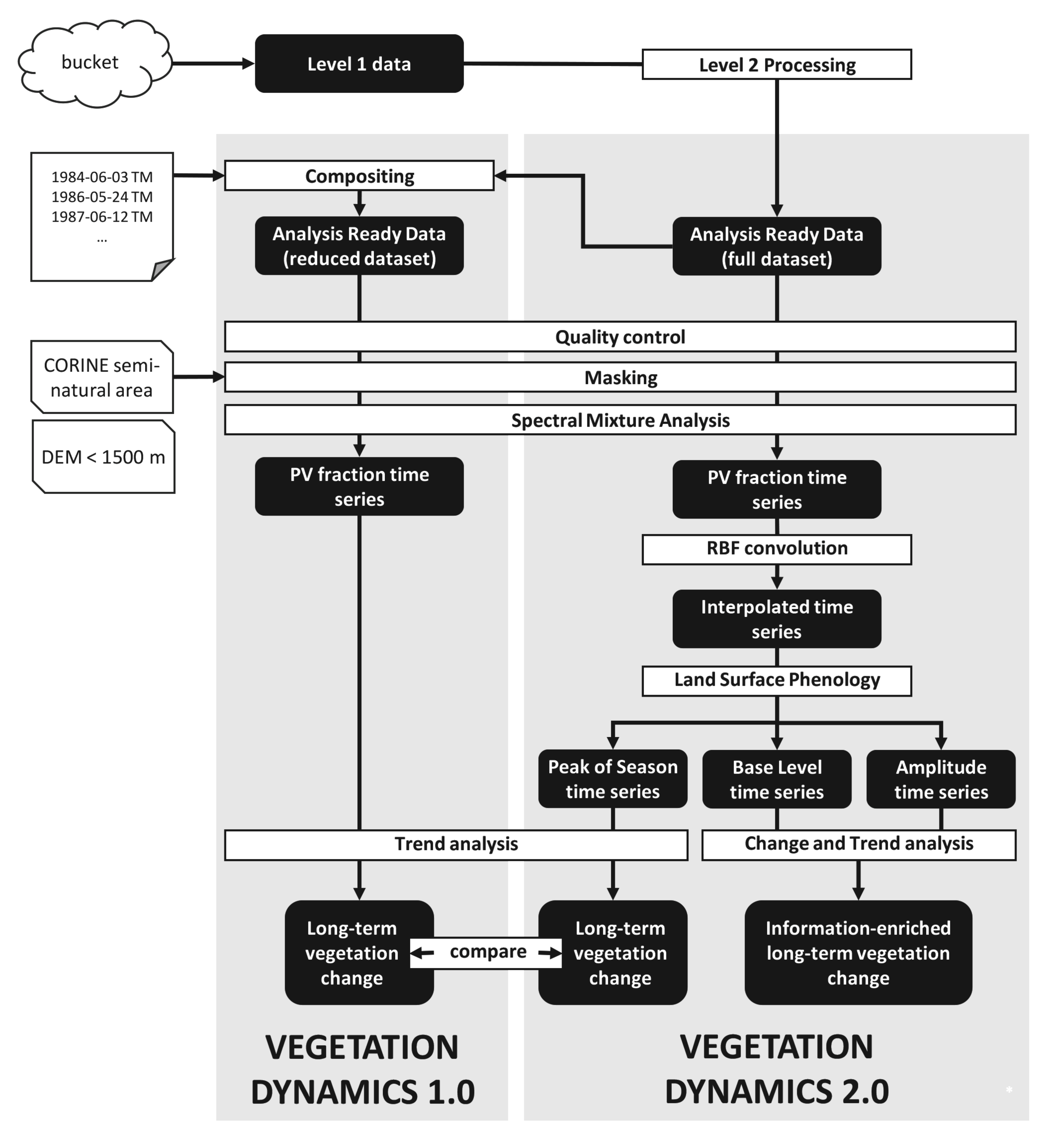
Most processing outlined in this section was performed using FORCE [59], freely available from https://github.com/davidfrantz/force, accessed on 18 September 2021. As outlined in the objectives, we processed and analyzed the data with two different methods, one to reproduce the past state-of-the-art with few input data (hereby denoted as “Vegetation Dynamics 1.0”: VD 1.0), and the second to replicate with state-of-the-art methods and all available data (“Vegetation Dynamics 2.0”: VD 2.0–in the sense of [64]). After downloading the data, the complete VD 2.0 processing was performed in two steps only, equaling two user interactions (Figure 2). The first step was the generation of Analysis Ready Data (ARD), i.e., data preprocessed to allow immediate analysis with a minimum of additional user effort and guaranteed interoperability both through time and with other datasets (http://ceos.org/ard/, accessed on 18 September 2021). The second step comprised all higher-level processing carried out in the temporal domain, enabled by the data cube structure of the ARD that allows for immediate and efficient access to the temporal sequence of each pixel. The VD 1.0 processing was performed in FORCE, too, although some more user interactions were necessary to reproduce a workflow comparable to [42,49]. Postprocessing and validation were performed in R [65]. The complete workflow is outlined in Figure 2. All mathematical symbols used throughout the paper are listed in

Table 1. Mathematical symbols.

Symbol	Description	Symbol	Description
ΔD	Difference between selected observation and target date	[x,y]	Cartesian coordinates
ρ	Reflectance	[$\langle r\rangle$,$\langle f\rangle$]	Long-term average vector
Δρ	Residual between observed and interpolated reflectance	[$\langle x\rangle$,$\langle y\rangle$]	Long-term average of Cartesian coordinates
b	Spectral band	$\langle \theta \rangle$	Typical (long-term) start of the phenological year
F	Fractional cover	s, ns	Season, number of seasons
f	Shade-normalized fractional cover of photosynthetically active vegetation	[$\overline{r_s}$, $\overline{f_s}$]	Seasonal average vector
E	Model error	[$\overline{x_s}$, $\overline{y_s}$]	Seasonal average of Cartesian coordinates
t	Time	$\overline{{\theta }_s}$	Start of the phenological year in season
Δt	Time difference	y, ny	Calendar year, number of years
n	Length of the time series	fVPS,y	Annual peak of season fractional cover
ε	Noise of the time series	fVBL,y	Annual fractional cover seasonal base level
w	Weight	fVSA,y	Annual fractional cover seasonal amplitude
σ	Sigma of Gaussian bell	a, b	Regression intercept and slope
DOY	Day of the Year	CC	Relative cover change
[r,f]	Polar coordinates (Day of the Year in radians, fraction)	CCnet	Absolute net cover change

.

3.1. Step 1: Analysis-Ready Data (ARD)

3.1.1. Preprocessing of the Full Dataset

All Landsat images were converted to ARD using the FORCE Level 2 Processing System (v. 3.5). Clouds and cloud shadows were identified using a modified version of the Fmask algorithm [57,66,67,68]. The cloud masking is currently assessed in the Cloud Masking Inter-comparison Exercise (CMIX, https://earth.esa.int/web/sppa/meetings-workshops/hosted-and-co-sponsored-meetings/acix-ii-cmix, accessed on 18 September 2021) as well as in [69]. The FORCE atmospheric correction [68] branched from the AtcPro algorithm [50] used in the reference studies, and was re-implemented to enable bulk-processing of large image volumes [70]; thus a high level of comparability is ensured. The images were radiometrically standardized using radiative transfer modeling [71], including object-based Aerosol Optical Depth (AOD) estimation over dense dark vegetation [72] and water features [73]. Water vapor absorption was corrected using nearly concurrent MODIS water vapor estimates [74] or a long-term climatology as an approximation [62]; the effect of using the climatology as a surrogate was recently assessed in [63]. AOD estimation, as well as surface reflectance retrieval, were assessed in the Atmospheric Correction Inter-comparison Exercise (ACIX) [75], as well as in the ongoing 2nd edition (ACIX-II, https://earth.esa.int/web/sppa/meetings-workshops/hosted-and-co-sponsored-meetings/acix-ii-cmix, accessed on 18 September 2021). Topographic correction was performed with an enhanced C-correction, wherein the C-factor was estimated for each pixel in the image, then propagated through the spectrum using radiative transfer [76]. Three kernels of increasing size were used to approximate the background reflectance for adjacency effect correction [77]. Nadir BRDF-adjusted reflectance was retrieved using a global set of MODIS-derived BRDF kernel parameters [78]. Eventually, all images were re-projected to a single coordinate system (EPSG:3035) and then split into 30 × 30 km² image chips using a custom grid, thus representing data cubes [79]. This data cube concept allows for non-redundant data storage, efficient data access, as well as simplified extraction of data and information, which is required for the higher level processing outlined in the following sections.

3.1.2. Dataset Reduction for Vegetation Dynamics 1.0

Before the opening of the Landsat archive, VD 1.0 studies were limited to few Landsat images that needed to be handpicked carefully. Sonnenschein et al. [49] manually selected 14 Landsat TM/ETM+ images from 1984–2005 based on cloud cover and seasonal constraints with a maximum gap of one year between acquisitions (

Table 2. Target dates used for Vegetation Dynamics 1.0 and pixel share of selected observations relative to the target dates (ΔD).

Target Date	ΔD = 0	ΔD = −9	ΔD = −1	ΔD = +7	ΔD = Other
Unit	(%)	(%)	(%)	(%)	(%)
1984-06-03	66.60	5.37	0.00	28.02	0.02
1986-05-24	69.45	0.00	0.00	30.54	0.01
1987-06-12	65.56	0.01	0.00	34.39	0.04
1988-05-29	67.08	0.03	32.86	0.01	0.02
1989-06-17	67.88	0.00	0.00	32.11	0.01
1991-05-22	67.60	0.00	0.00	32.36	0.03
1993-05-27	67.66	10.85	0.00	21.48	0.00
1994-05-30	68.71	0.01	0.00	31.25	0.03
1996-06-04	64.96	0.01	0.00	35.03	0.00
1997-05-22	64.03	0.02	0.00	35.95	0.00
2000-05-30	67.21	0.02	32.76	0.01	0.00
2002-05-28	67.35	30.31	0.00	0.00	2.34
2004-06-10	66.00	0.02	0.00	33.96	0.01
2005-06-13	67.19	9.19	0.00	23.57	0.04

). They aimed to pick images at peak vegetation vigor, which was assumed to approximately correspond to mid-May to mid-June in the mountainous rangelands of Crete. The seasonal validity of each selected image was compared with a 10-day AVHRR NDVI time series [80] for selected plots in these rangelands. To mimic this hand-picking of images, but for the whole of Crete, we used a selection algorithm on the full ARD dataset. We generated pixel-based composites with a parametric weighting scheme [15,22] with the FORCE Higher Level Processing System (v. 3.5) using the seasonal proxy as the only determinant, i.e., the closest observation to a target date was used to populate each pixel in the composite. The selected acquisition dates (Table 2) were used as temporal targets, and a narrow compositing period of ±10 days was used to restrain the selection of observations to dates that are as close as possible to the target dates. For most pixels, the exact date was selected, with secondary peaks at +7, −1, and −9 days, which are related to Landsat’s orbital paths. Note that these composites still contain some clouds as only the seasonal suitability was used as the selection criterion. This was done to ensure that the compositing algorithm is biased towards selecting full images as this matches the manual selection process from the reference studies. Still, clouds were masked out for the analysis using the automated cloud masks, whereas clouds were manually identified in the reference studies.

3.2. Step 2: Time Series Analysis

The second step was performed with the FORCE Higher Level Processing System (v. 3.7), which includes a time series analysis submodule that may be configured to chain the following sub-sections in a single execution with one user interaction only.

3.2.1. Spectral Unmixing

For each acquisition date—the full dataset for VD 2.0, the reduced dataset for VD 1.0—an ecologically reasonable index for representing vegetation cover was computed based on the bottom-of-atmosphere reflectance spectra. Spectral Mixture Analysis (SMA, see for example, Somers et al. [81] for an overview) is superior compared to vegetation indices in quantifying sparse vegetation cover over bright background materials [82,83]. For comparability with Hostert et al. [42], and as we deem conventional SMA a straightforward means to generate consistent vegetation fractions for long and dense time series, we employed a linear unmixing approach following:

$${\rho }_b={{\displaystyle \sum }}_{i=1}^m{F}_i·{\rho }_{i,b}+E_b,$$

(1)

wherein band-wise reflectance ρ_b is explained as the summarized product of m endmember reflectance spectra ρ_i,b with their respective fractions F_i. A least-squares optimization was performed to minimize the model error E_b [83], while both enforcing non-negativity of fractions F_i [84], and honoring the sum-to-one constraint

$${{\displaystyle \sum }}_{i=1}^m{F}_i=1.$$

(2)

For congruency with Hostert et al. [42], we selected the same reference endmembers from field measurements (

Table 3. Endmember set derived from [42]; values are in percentage reflectance.

Spectral Band	Photosynthetic Active Vegetation	Soil	Rock	Shade
Blue	3.2	7.3	26.2	0.0
Green	5.6	14.5	31.0	0.0
Red	4.5	22.4	33.4	0.0
NIR	36.7	27.5	47.0	0.0
SWIR1	17.0	40.2	72.4	0.0
SWIR2	7.1	32.2	54.9	0.0

), i.e., rock (limestone with lichen), soil (Luvisol), photosynthetically active vegetation (PV, Quercus coccifera), and spectrometric shade for scaling the fractions for physical interpretability (Equation (3)). The four-endmember model was carefully selected considering the inherent dimensionality of Landsat TM data [42]. The limitation to four endmembers leads to non-photosynthetic vegetation (NPV) falling into the soil fraction component. This does not affect our comparison, given that the interpretation focuses on the trends in photosynthetic active vegetation here. The derived PV fraction was used for all further analyses. For simplicity, we will use f without subscript to refer to the shade-normalized PV fraction for the remainder of the manuscript.

$$f=F_{PV}/\left(1-F_{Shade}\right).$$

(3)

3.2.2. Land Surface Phenology for Vegetation Dynamics 2.0

For the VD 2.0 analysis, additional processing was performed to generate annual time series devoid of seasonal effects that may arise from the static selection.

With LGAC data migration and data restoration of imagery lacking payload-correction data, it is generally feasible to extract the timing of specific phenological key points from the full data record on a per-pixel basis, i.e., to derive land surface phenology (LSP) metrics directly [32], or to downscale coarse resolution LSP metrics using data fusion techniques [85].

In a first step, the quality bit product was used to remove all poor-quality observations, i.e., pixels flagged as cloud, cloud shadow, snow, as well as saturated or sub-zero reflectance values. Acknowledging that cloud, and especially cloud shadow masks, are not perfectly accurate, a time series-based outlier detection followed by an inlier restoration was performed based on the noise estimation proposed by Vermote et al. [86]. Given a triplet of successive observations, the absolute residual r between the central observation i and linear interpolation between its neighbors is given by:

$$r_i=\left|{\rho }_i-\frac{{\rho }_{i+1}-{\rho }_{i-1}}{t_{i+1}-t_{i-1}}·\left(t_i-t_{i-1}\right)-{\rho }_{i-1}\right|,$$

(4)

where ρ is the reflectance of the shortest wavelength, i.e., blue, which commonly is most severely affected by remaining noise due to atmospheric effects; t is the time measured in continuous days. The noise ε of a time series with n observations is estimated as:

$$\epsilon =\sqrt{{{\displaystyle \sum }}_{i=2}^{n-1}{r}_i/n-2}.$$

(5)

We iteratively removed the observation i with the largest residual r_i,max, if r_i,max/ε exceeded a threshold. Subsequently, we restored all observations that were eliminated via the quality bit product, if r/ε was below a threshold. We set these thresholds to 3 and 1, respectively, which were found to be reasonable values based on practical experience.

Subsequently, the f time series were interpolated using an ensemble of Radial Basis Function convolution (i.e., smoothing) filters as described by Schwieder et al. [87], where the observations in the kernel are weighted according to a Gaussian distribution:

$$w_t=\frac{1}{\sigma ·\sqrt{2\pi }}·\exp \left(-0.5·{\left(\frac{\Delta t}{\sigma }\right)}^2\right),$$

(6)

with t being the time of the observation, Δt the observation time relative to the kernel center, and σ the full-width-at-half-maximum of the Gaussian bell-shaped curve, all values given in days. We used three kernel widths σ with 8, 16, and 32 days, as e.g., employed by Rufin et al. [88]. A kernel cutoff value that preserves 95% of the area under the Gaussian curve was used. The estimates from the three kernels were eventually aggregated using a weighted average, wherein the weights correspond to the data available within each kernel. This weighting strategy gives preference to kernels with a higher data density for the final value estimation. Due to the implemented kernel cutoff value, no-data values occasionally remained during the winter season when data gaps are substantially larger than the employed kernel widths, and as such, we subsequently performed a linear interpolation to strictly enforce equidistance and absence of data gaps.

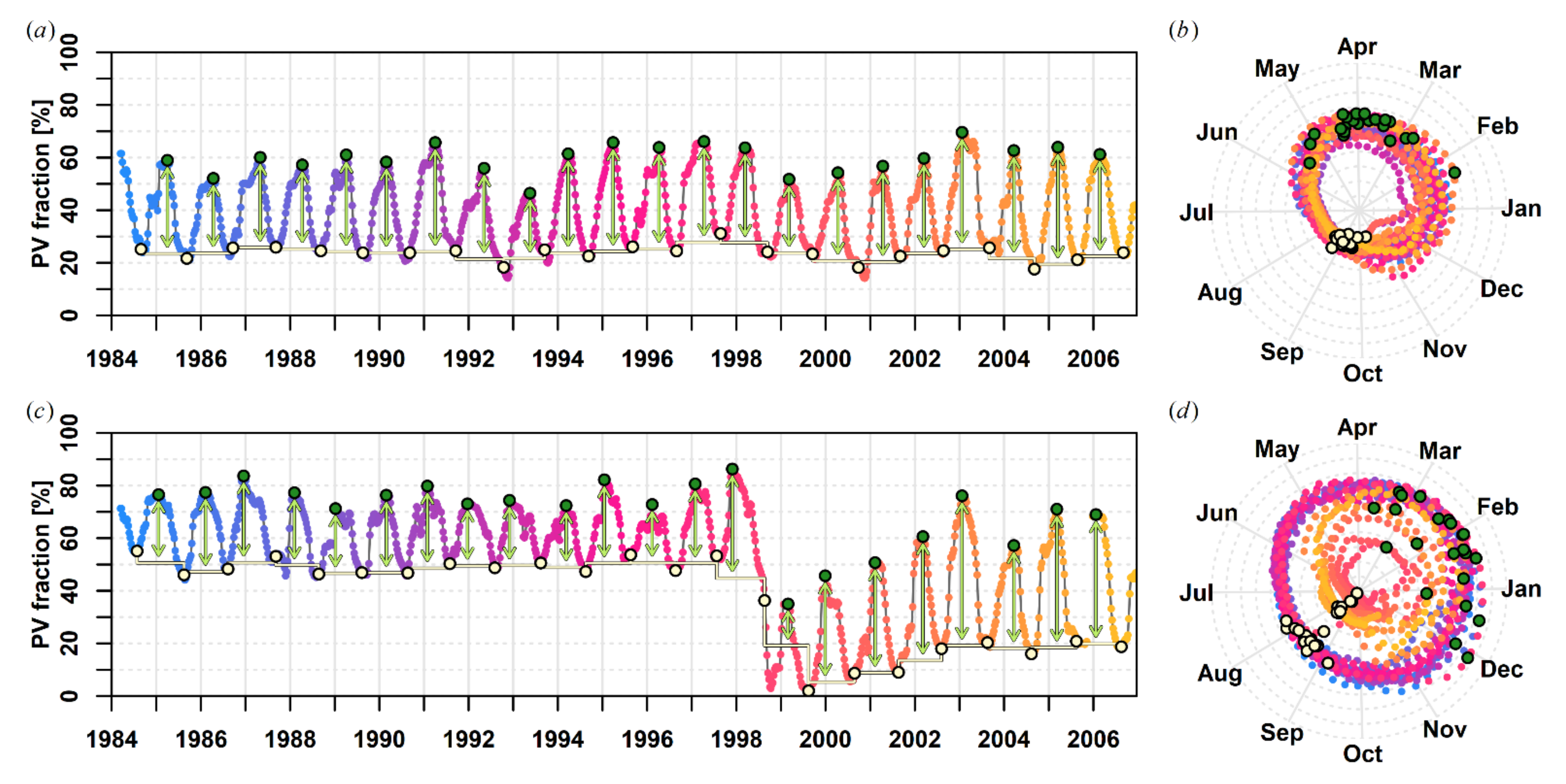
LSP metrics for each year between 1984 and 2006 were then derived from the interpolated time series using a polar transformation-based methodology based on the concept proposed by Brooks et al. [33], partially reproduced here for the sake of readability. The time series is transformed into polar space by converting DOY to radians:

$$r_t=DO{Y}_t/365.0·2\pi .$$

(7)

Polar coordinates are then transformed to Cartesian space (Figure 3) using:

$$\begin{array}{c}{x}_{r,f}=f_t·\cos r_t\\ y_{r,f}=f_t·\sin r_t\end{array}$$

(8)

and the long-term polar average vector [$\langle r\rangle$,$\langle f\rangle$] is computed from the average Cartesian coordinates [$\langle x\rangle$,$\langle y\rangle$] as:

$$\langle r\rangle =\left\{\begin{array}{c}atan2\left(\langle y\rangle ,\langle x\rangle \right) \\ atan2\left(\langle y\rangle ,\langle x\rangle \right)+2\pi \end{array}\right.\begin{array}{c}atan2\left(\langle y\rangle ,\langle x\rangle \right)>0\\ otherwise\end{array},$$

(9)

$$\langle f\rangle =\sqrt{{\langle x\rangle }^2+{\langle y\rangle }^2}.$$

(10)

The long-term average vector points to the direction of the central tendency of annual peak cover. As phenological timing can substantially vary from pixel to pixel due to environmental and biophysical characteristics, the typical start of the phenological year $\langle \theta \rangle$ is computed as the diametric opposite angle of [$\langle r\rangle$,$\langle f\rangle$], which points into the direction of least annual cover:

$$\langle \theta \rangle =\left\{\begin{array}{l}\langle r\rangle +\pi \\ \langle r\rangle -\pi \end{array}\right.\begin{array}{l}\langle r\rangle <\pi \\ otherwise\end{array}$$

(11)

This long-term measure of the start of the phenological year is used to structure the time series into phenological years, i.e., annual slices that contain a full season. Besides spatial variability, inter-annual variability may be substantial when analyzing highly volatile, precipitation-driven phenologies, such as in the Mediterranean. As such, we further improved on the Brooks method by fine-tuning the start of the phenological year for each season. For this, we use the initial long-term start of the phenological year $\langle \theta \rangle$, and re-estimate $\overline{{\theta }_s}$ for each season s (Equations (9)–(11)). This is achieved by considering $\overline{{\theta }_s}$ as the diametric opposite angle to the seasonal average vector [$\overline{r_s}$, $\overline{f_s}$], which is computed from the average of all Cartesian coordinates [$\overline{x_s}$, $\overline{y_s}$] in the given season (i.e., the annual slices between $\langle \theta \rangle$). The updated values $\overline{{\theta }_s}$ are then used to restructure the time series into phenological years with a dynamic, yet reasonably constrained, phenological offset.

The observations before $\overline{{\theta }_1}$ and after $\overline{{\theta }_{ns}}$ in the first and last season of the time series, respectively, need to be discarded as they do not represent a full phenological cycle; thus resulting in ns = ny − 1 seasons, where ny is the number of years in the time series. If $\langle \theta \rangle$ is located in the first half of the year, we did not obtain LSP metrics for the last year; or the 1st year if otherwise. Once the time series was structured into years, the computation of LSP metrics was straightforward, and a multitude of parameters that describe the timing of phenological key events, seasonal variability, seasonal bimodality, etc. were implemented in FORCE (see https://force-eo.readthedocs.io/en/latest/components/higher-level/tsa/format.html#phenology, accessed on 18 September 2021, for a complete list).

Our reference studies aimed at selecting images at peak vegetation vigor. Thus, in a first step, we focused on the value of peak of season (VPS) metric, which is the maximum fractional cover for each year f_VPS,y (see Figure 3) representing the fractional cover of all photosynthetically active vegetation types (PV).

On Crete, vegetation growth below the alpine zone is not limited by temperature, but by water availability: woody vegetation is predominantly evergreen, and thus a fairly constant photosynthetically active fractional cover persists throughout the year, while the seasonal growth in woody vegetation is relatively small. In contrast, herbaceous vegetation has a strong seasonal component, where photosynthetically active fractional cover rapidly increases in response to winter rainfall and then quickly turns into NPV at the beginning of the hot and dry summer. Thus, in the second step, we additionally selected LSP metrics that approximate the seasonal growth of these vegetation components, and consequently offer a decomposition of the total PV cover into woody and herbaceous components. The value of base-level (VBL) is defined as the minimum fractional cover of each year f_VBL,y, computed as the average of the first fractional cover value after $\overline{{\theta }_s}$ and $\overline{{\theta }_{s+1}}$, and hence approximates the fairly stable fractional cover of woody vegetation. The value of seasonal amplitude (VSA) is the difference between VPS and VBL: f_VSA,y, thus f_VPS,y = f_VBL,y + f_VSA,y. It approximates the seasonal growth of PV cover and is thus well aligned with the seasonal dynamics of herbaceous vegetation. It further follows that the remainder represents other cover types (soil, rock, or non-photosynthetically active vegetation), i.e., F_NS = 1.0 − (f_VBL,y + f_VSA,y).

3.2.3. Trend Analysis

For both VD 1.0 and VD 2.0, pixel-based linear trend analyses were performed on the annual time series:

$$f=a+b·y,$$

(12)

with regression intercept a and slope b. For VD 1.0, the trend analysis was performed on f derived from the reduced ARD dataset. We accounted for shifts in acquisition times by setting the regression time scale to fractional years since 1984, i.e., the middle of 1984 and the beginning of 1986 are encoded as y = 0.5 and y = 2.0, respectively. For VD 2.0, the trend analysis was performed on the annual f_VPS values, thus the time scale for this analysis was simply given in years since 1984. As identical change magnitudes (trend b) have a substantially different meaning depending on the initial cover (offset a), we further normalized the trends to represent cover change CC (%), which is the long-term cover loss/gain measured relative to the initial cover:

$$CC=100·\left(b·ny\right)/a.$$

(13)

3.2.4. Trend + Change Analysis

Disturbances in the woody vegetation component result in a non-linear trajectory of vegetation cover, and as such, linear trend analysis alone is ill-suited for these cases. Consequently, we further used an extension of the Change, Aftereffect, and Trend (CAT) transformation [37]. The original CAT transformation produces three parameters, which were primarily chosen for a synoptic visualization of landscape change processes as RGB composite. Given an annual time series of a vegetation index, Change is the maximum absolute difference between consecutive years; Aftereffect is the mean value after the change; and Trend is the slope of a linear regression applied to the full annual time series.

We complemented the CAT concept with a more exhaustive set of change and trend parameters including three change parameters: change, year of change, and percentage loss, wherein change only considers negative changes and percentage loss is the change relative to the initial cover as estimated by the offset of a linear regression applied to the full annual time series (analogous to Equation (13)). In addition, a full set of trend parameters is generated for each part of the time series, i.e., before and after the change, as well as for the complete time series.

3.3. Postprocessing: Vegetation Dynamics Syndrome Classification

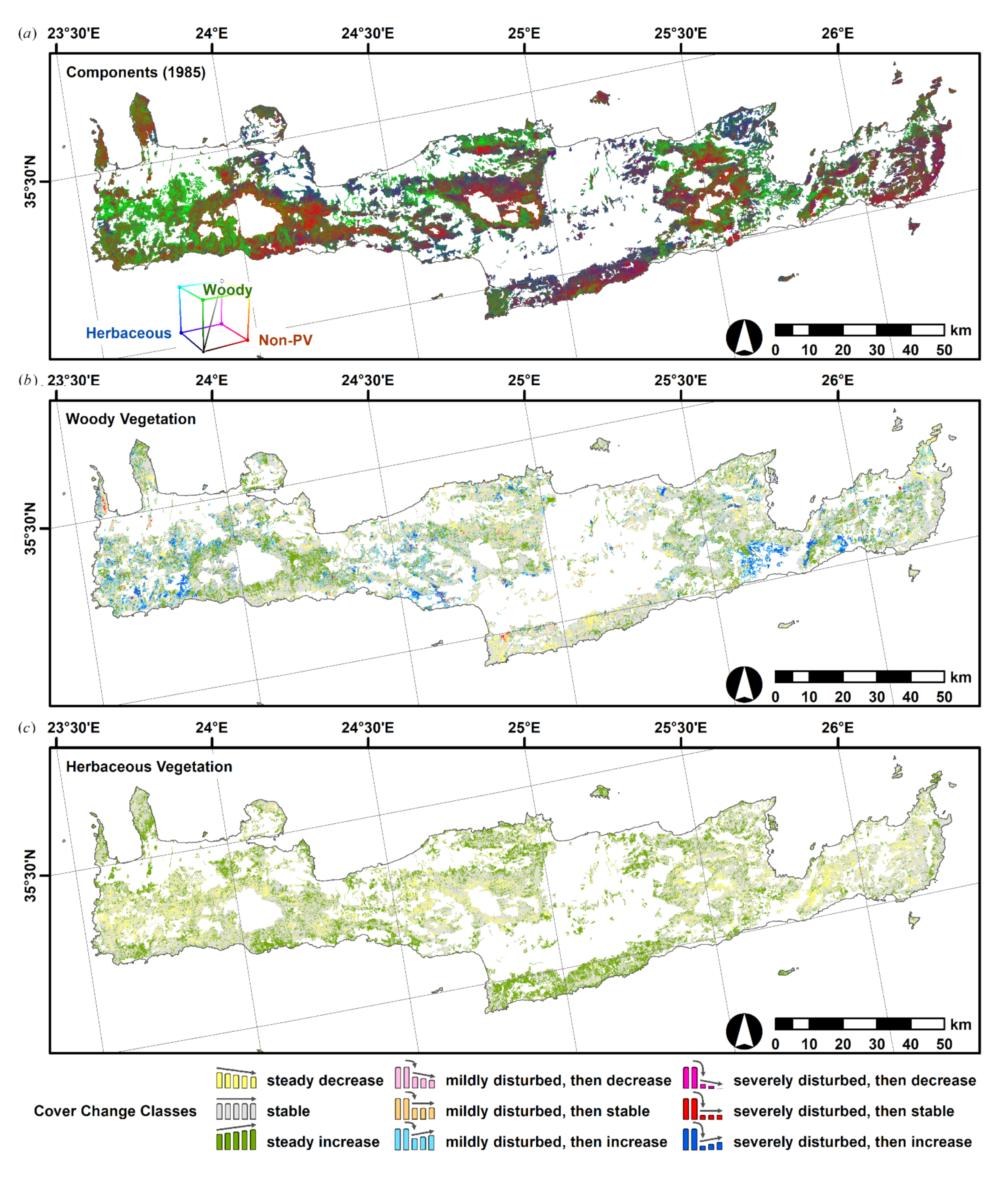
For the woody vegetation, we classified the VBL-based CAT parameters into nine classes using a simple expert-based decision tree (Figure 4) similar to the land-use change syndrome approach [34,35]. If the initial cover was above 25% and if more than 25% of the initial cover was lost abruptly, the pixel was labeled as being disturbed. These pixels were further divided into two disturbance severity classes (mildly and severely disturbed), as well as into three directional classes based on thresholds as used in Hostert et al. [42] of the trend component for the “after disturbance” segment, i.e., mild/severe disturbances followed by a decline, stagnation, or recovery of fractional cover. For non-disturbed pixels, three classes were labeled accordingly, but using the trend component of the full time series, i.e., steady decrease, steady increase, or stable fractional cover. The herbaceous vegetation cover has high inter-annual variability in response to the rainfall sum of the preceding rainy season. In addition, disturbance (e.g., fire) rarely results in a permanent loss of herbaceous vegetation, as it recovers quickly. As we are only investigating semi-natural areas, land cover changes from semi-natural to, for example, built-up or agriculture, are excluded. Consequently, only the gradual conditions were used for the herbaceous cover, i.e., the VSA-based CAT parameters were split into three gradual change classes (Figure 4). The combination of both layers allows for a more nuanced and information-enriched long-term vegetation change assessment for both the woody and herbaceous vegetation.

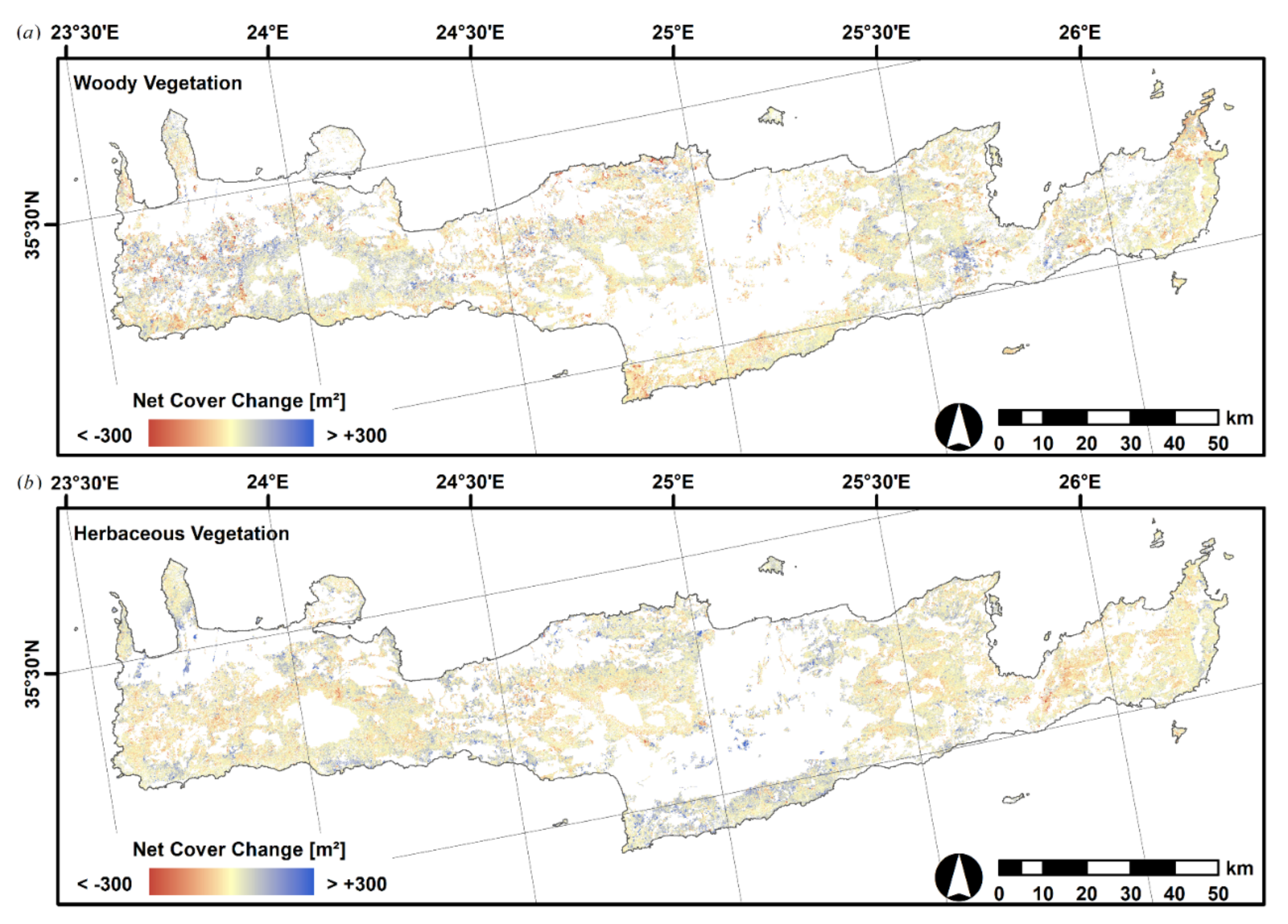
Additionally, the absolute net cover change (m²) was computed for each pixel and component. For pixels subject to gradual processes, the net cover change was computed as the absolute gain/loss for the complete period:

$$C{C}_{net,complete}=\left(b·ny\right)·900 {\mathrm{m}}^2.$$

(14)

For disturbed pixels, the net cover change was computed as the sum of the three parts of the time series following the CAT transform:

$$C{C}_{net,disturbed}=C{C}_{net,before}-C{C}_{net,change}+C{C}_{net,after},$$

(15)

with:

$$\begin{array}{c}C{C}_{net,before}=\left(b_{before}·n{y}_{before}\right)·900 {\mathrm{m}}^2\\ C{C}_{net,change}=\left(Change\right)·900 {\mathrm{m}}^2\\ C{C}_{net,after}=\left(b_{after}·n{y}_{after}\right)·900 {\mathrm{m}}^2\end{array}$$

(16)

3.4. Validation

Validation data on vegetation components and their fractional cover, as well as long-term trends thereof, are unfortunately not available for the study area and cannot easily be derived from existing data sources. This especially applies as a result of the historic investigation period with unavailability of very high-resolution imagery, which would be needed at multiple time steps. Moreover, the mixed pixel spectral signatures dominating our feature space, and subtle changes thereof, prevent the development of quantitative reference data from the medium-resolution data themselves. A discussion on challenges considering a reliable, historic validation can be found in Hostert et al. [43]. In order to still provide guidance on the reliability of our used methods, we implemented a verification strategy based on interactive time series interpretation. As we needed to validate and compare different information layers of both quantitative and qualitative datatypes, we drew a random sample across Crete and evaluated all layers at the same point locations. We used Poisson Disc Sampling [89], a sampling technique that provides a uniform sample distribution across the study area with minimum distance between points; N = 977 samples were obtained. A trained expert was handed validation sheets with time series of the employed Landsat data, superimposed with the derived trends for the VD1.0 and VD2.0 analyses, peak of season, base level, and seasonal amplitude metrics, as well as detected changes and trends of the woody and herbaceous vegetation components. Annual subsets of best available pixel composites were plotted to provide spatial context. The expert assessed whether the outputs of the algorithm were obviously erroneous to the human eye, e.g., whether an illogical trend was computed, the magnitude was unreasonable, or whether a spurious change was detected. This may include incorrect trend magnitude or even trend direction due to misalignment of the VD1.0 date selection with the actual timing of peak phenology, exaggerated or reduced trend magnitudes which can be caused by incorrect offsets in result of missing data towards the beginning or end of the time series, or spurious change caused by missing or erroneous data. The assessment either confirmed or rejected the results of (1) the VD 1.0 and VD 2.0 trend analysis on total vegetation cover, (2) the change component of the woody vegetation cover, (3) the trend component of the woody vegetation cover, and (4) the trend analysis of the herbaceous vegetation cover.

4. Results and Discussion

All maps presented in the following are available through an interactive web viewer: https://ows.geo.hu-berlin.de/webviewer/crete/ accessed on 18 September 2021; note that the vegetation components map for 1984, i.e., the first year of available data, is incomplete as a full phenological cycle need to exist to extract LSP metrics (see Section 3.2.2). The dataset produced in this study can be accessed at https://zenodo.org/record/5902672#.YfENz-rMKCo, accessed on 18 September 2021.

4.1. Comparison of Long-Term Vegetation Change between Vegetation Dynamics 1.0 and Vegetation Dynamics 2.0

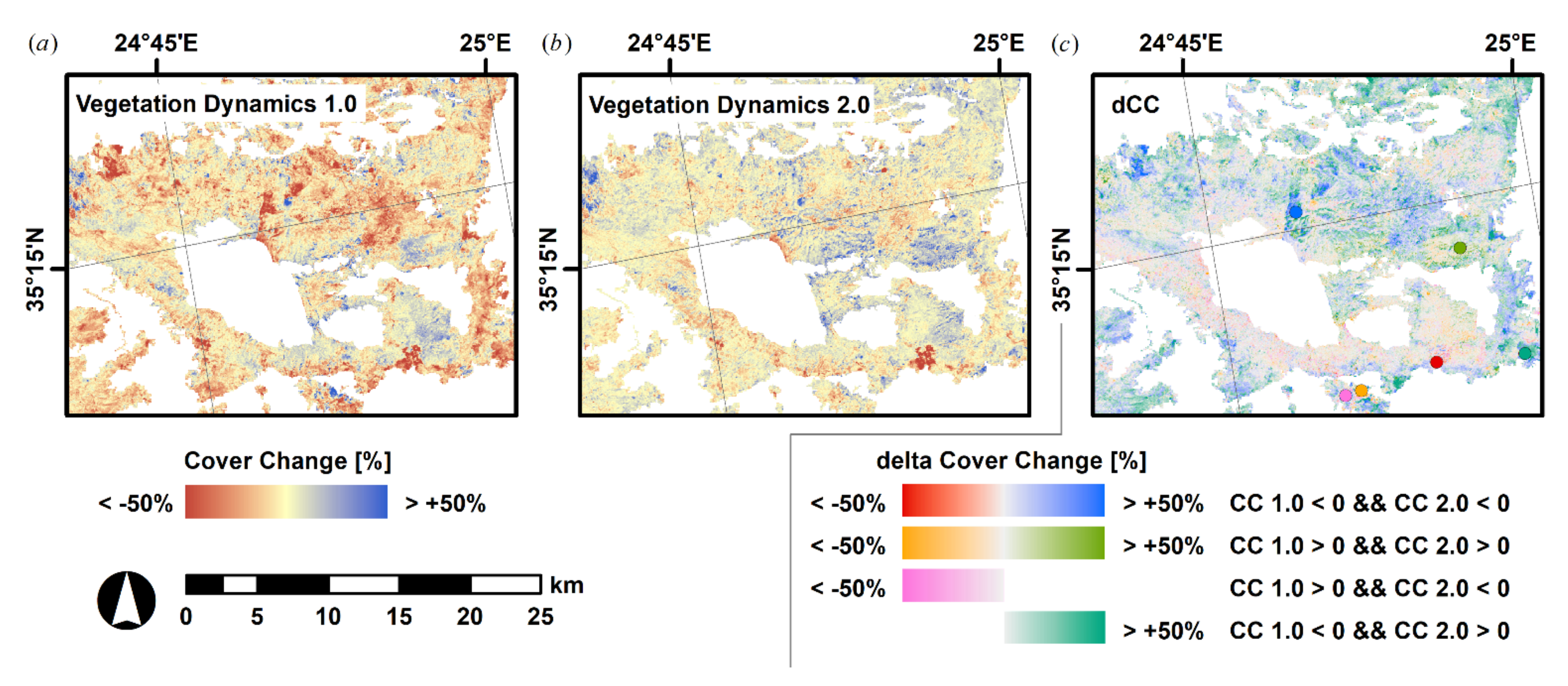
The long-term vegetation cover change maps of the reproduced VD 1.0 indicate large areas with severe cover loss, Figure 5a. Overall, net change over Crete is negative (

Table 4. Area statistics of cover change for the Vegetation Dynamics 1.0 and Vegetation Dynamics 2.0 analyses.

Category	Cover Change Class (%)	Proportion Vegetation Dynamics 1.0		Proportion Vegetation Dynamics 2.0
		(%)	(km2)	(%)	(km2)
Severe decrease	<−15	27.92	1212	5.63	245
Decrease	−15 to −5	21.88	950	12.43	541
Unchanged	−5 to +5	23.82	1034	31.55	1373
Increase	+5 to +15	15.18	659	29.34	1277
Strong increase	>+15	11.21	487	21.05	916

) with 50% and 26% of semi-natural areas showing signs of vegetation decline and increase, respectively. Although not numerically comparable (due to several reasons discussed in Section 1.1), these numbers resemble the findings in Hostert et al. [42], who found that over 40% of the mountain area of central Crete (Psiloritis) showed a decreasing trend of vegetation cover. Spatial patterns are also very similar to the maps published by Sonnenschein et al. [49], both indicating that general reproducibility with the past papers is given from a thematic perspective with a focus on overgrazing and that similar conclusions would have been drawn as before.

However, the results from VD 2.0 are fundamentally different to those from VD 1.0 (Figure 5b). Severe cover loss is limited to small areas and the magnitude of cover change is smaller compared to VD 1.0. Overall, net cover change is positive with 18% of areas showing a decreasing trend of vegetation cover, while half (50%) of all semi-natural areas exhibit an increase (Table 4).

As the Psiloritis mountains were the primary study area in our reference studies, Figure 6 closes in on this area, and further depicts the difference in cover change ΔCC between both methods:

$$\Delta CC=C{C}_{2.0}-C{C}_{1.0}.$$

(17)

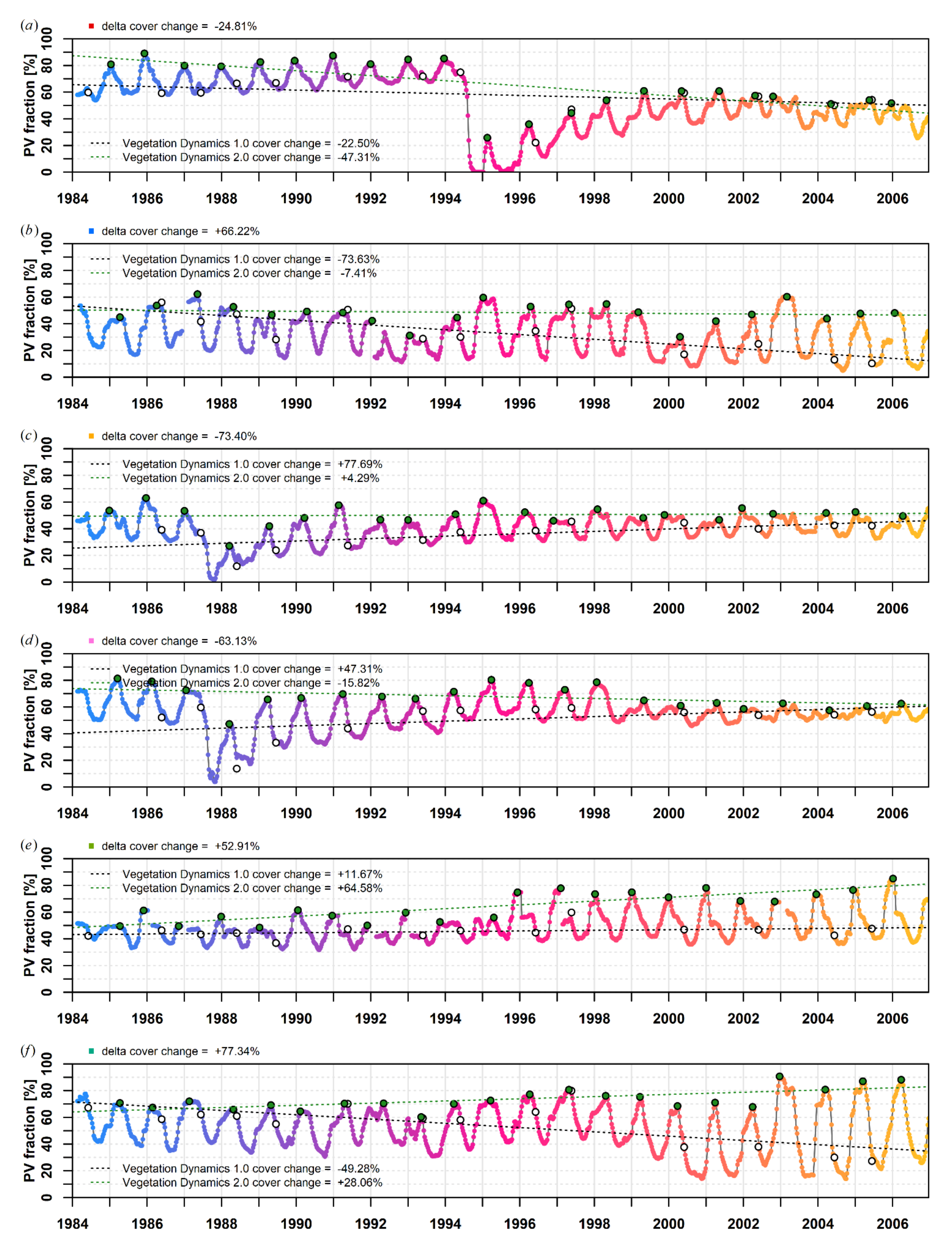
ΔCC can assume the same value for different combinations of trend directions; as such, Figure 6c ΔCC is styled with four separate color bars. The first two color bars represent areas where the trend direction is consistent, the last two color bars represent areas with opposite trend directions. Figure 7 shows representative pixel time series, along with trends, for the six different colors in Figure 6c. The comparison of VD 1.0 and VD 2.0 reveals several general observations:

• For both-negative trends, VD 2.0 rarely indicates a stronger decline (red in Figure 6c); Figure 7a shows a pixel where a fire occurred. The disagreement between methods is due to several reasons: (1) in the year where the change happened, no cloud-free image was available in VD 1.0, thus the fresh disturbance scar is not included in the regression; (2) before the change, the statically selected images coincide more closely with minimal cover, whereas they coincide more closely with peak cover thereafter—presumably due to a change in vegetation composition after the disturbance.
• More commonly, however, VD 1.0 shows stronger negative trends (blue in Figure 6c, cf. Figure 7b). The trajectory shows large inter-annual variability with a low annual minimum of PV fractions, thus pointing to herbaceous-dominated vegetation composition. For such pixels, the static VD 1.0 image selection results in a volatile timing of the observation relative to the phenological cycle—sometimes close to peak cover, sometimes close to minimal cover. Thus, the resulting trend needs to be considered error-prone and potentially spurious. However, it is also apparent that, although the peak vegetation cover is rather stable over the long period (VD 2.0), there still is change related to a decreasing annual minimum of the cover, which is largely balanced by an increase in seasonal amplitude. This could be caused by an increase in herbaceous cover at the expense of a woody cover.
• Orange colors in Figure 6c represent pixels where both trends are positive with a stronger increase in VD 1.0; pink colors in Figure 6c represent pixels with a positive trend in VD 1.0 and a negative trend in VD 2.0. In both time series, a change is included that transiently (Figure 7c) or progressively (Figure 7d) modifies the vegetation composition such that static image selection does not guarantee a stable location of the observation relative to the phenological cycle.
• Green colors in Figure 6c represent pixels where both trends are positive with a stronger increase in VD 2.0; teal colors in Figure 6c represent pixels with a negative trend in VD 1.0 and a positive trend in VD 2.0. The corresponding time series (cf. Figure 7e,f) reveal that there is indeed an increase in peak cover (VD 2.0). The VD 1.0 analysis, however, indicates a slight increase only (Figure 7e) or a strong decline (Figure 7f), which is caused by a systematic shift in the timing of the statically selected images relative to the phenological cycle as a consequence of changes in vegetation composition towards a higher share of herbaceous cover, i.e., earlier peak cover that quickly turns into NPV at the beginning of the dry Mediterranean summer.

Our validation supports the above observations. Only 32.9% of samples in case of VD 1.0 were confirmed, whereas 98.7% of samples were positively evaluated for VD 2.0, which:

• corroborates the finding that static image selection is volatile in areas where inter-annual or spatial variability in phenology is high, and
• confirms the robustness of a data-driven approach using phenological metrics.

However, it also needs to be noted that the expert could not arrive at a decision in 4.4% of cases (for both VD 1.0 and VD 2.0), primarily because disturbances were present, in which case the expert could not reliably judge the results of a monotonic trend fitted through the full time series.

4.2. Information-Enriched Long-Term Vegetation Change

The LSP-based decomposition of total photosynthetically active vegetation cover into herbaceous and woody components is visualized in Figure 8a for the year 1985. Compared to the total vegetation cover (the sum of blue and green), this split offers another layer of interpretation that readily depicts areas with different vegetation compositions. It is important to note that this split does not produce meaningful results when the underlying assumptions are violated (cf. Section 3.2.2, e.g., for a deciduous forest with a substantial seasonal component, as well as lush grasslands in more protected pockets that do not entirely dry out during summer. These areas are very rare in Crete though, thus we believe that the decomposition provides reliable results at large. The decomposition is highly informative when paired with a trend-and-change analysis, followed by syndrome-based labeling of vegetation dynamics classes (Figure 8b,c; Table 4). Half of Crete’s semi-natural areas (i.e., cells of 30 × 30 km²) do not show substantial changes in woody cover (52%), whereas 8.5% and 19% are subject to gradual decreases and increases, respectively. The remaining 20% were disturbed, and almost half of these were on a recovery trajectory thereafter. The ongoing decline after a disturbance is fairly rare. More than half of all areas do not show strong changes in the herbaceous cover (56.5%), while 15.5% and 28% of the pixels show signs of decreasing and increasing cover, respectively.

The accuracy assessment of the syndromes reveals that severe disturbances in the woody vegetation, as well as the absence of a disturbance were detected with high quality. Mild disturbances, however, were detected less reliably such that our expert only confirmed 62% of these algorithmic decisions. In addition, 3.68% of all samples were not labeled as the expert could not make a reliable decision. The trend of the woody vegetation was only assessed for samples where the change detection was positively evaluated, thus reducing the sample size by 99; another eight samples were not labeled as the expert could not make a reliable decision. The trend component, both for the total length of the time series (in case no change was detected), and for the time after a disturbance were confirmed to be of high quality. The same is true for the trend analysis of the herbaceous vegetation. In both cases, the algorithmic decision was rejected in less than 1% of samples.

It is acknowledged that our validation is liberal in nature, as the interpreter had access to the algorithm’s decision and was tasked to reject decisions that did not match with human perception. Furthermore, this validation should only be interpreted in a qualitative sense, although our feature space (subpixel fractions of vegetation, annual LSP metrics), and observed change phenomena (long-term trends) are quantitative. Thus, it is to be expected that a more conservative validation with an independent and quantitative reference dataset would result in somewhat lower accuracies. However, such data on vegetation components and their fractional cover, as well as long-term trends thereof, are unfortunately not available for the study area, especially when considering the historic investigation period. This is similar to many other regions, where fractional cover reference data do not exist and cannot be created retrospectively either due to the non-existence of high resolution images at required temporal granularity, with Australia being an exception in terms of field data generation (but still for rather contemporary periods) [90]. Nevertheless, our quality assessment still underlines the robustness of this approach, and it is rooted in ecological principles of the seasonal pattern of photosynthetically active vegetation cover of woody and herbaceous vegetation components in semi-arid areas, see e.g., [91]. We therefore presume that our methodology is transferable to similar ecoregions with comparable data availability (although tuning of the endmember model might be necessary), e.g., to Australia, South Africa, or the Mediterranean at large. Due to the consistency of the contemporary and upcoming data from Landsat 8, Landsat 9, as well as Sentinel-2A/B and Sentinel-2C/D with the existing Landsat legacy data records, extending our approach temporally to the current era will be straightforward, too, although the change analysis may need to be extended (or interchanged with other tools, e.g., BFAST) to accommodate for more than one breakpoint. Our approach could also be extended using other novel approaches, e.g., by incorporating object-based segmentation of phenologically similar pixels to increase spatial coherence of spatially similar pixels [92] or by incorporating new insights of statistical trend estimates in large remote sensing data [93].

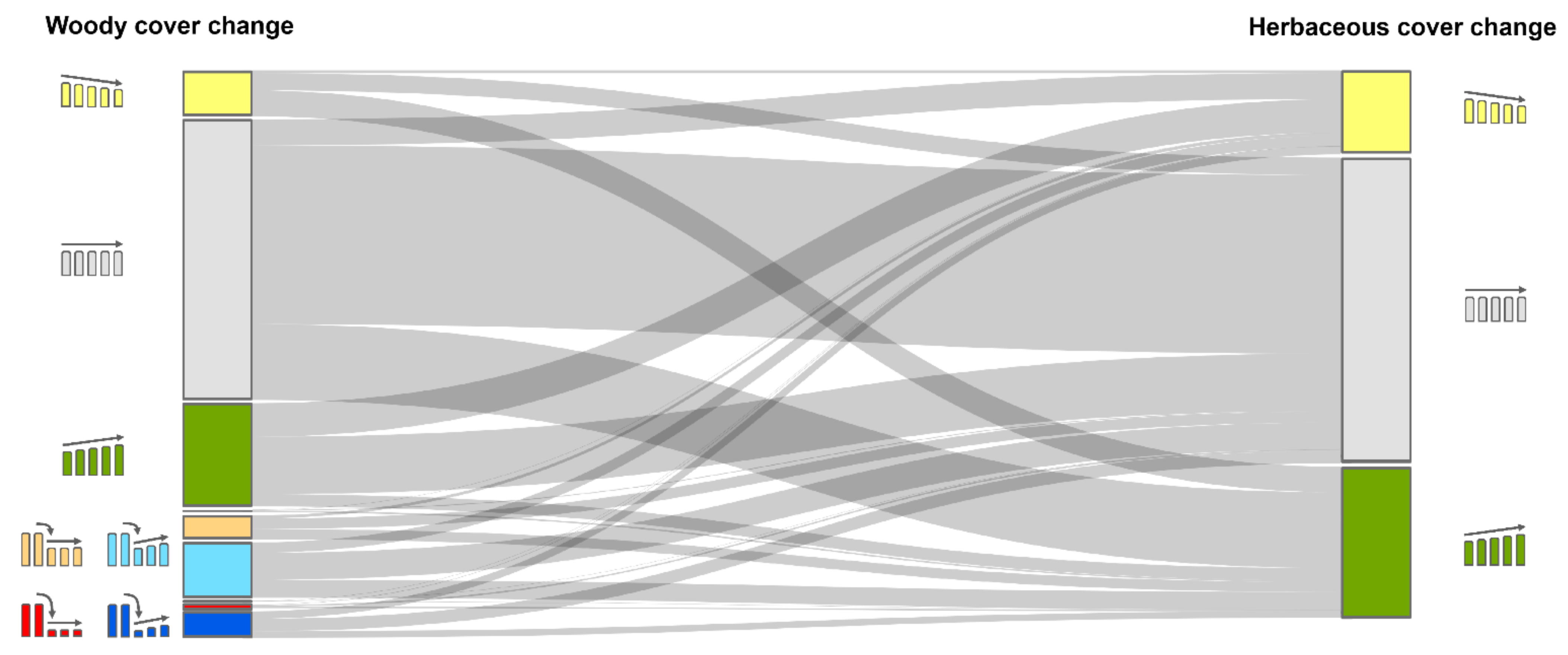
Entirely different drivers may relate to changes predominantly occurring in the herbaceous or woody cover, or a combination thereof (Figure 9). Thirty-eight percent of the areas with steadily decreasing woody cover (yellow left) do not show substantial changes in the herbaceous cover (gray right); 56% show signs of increasing herbaceous cover (green right). Thus, when only analyzing total vegetation cover as measured via the peak of season metric (Figure 5b), only the first case (yellow left, gray right) was observable. In the second case (yellow left, green right), the long-term decrease in woody cover was compensated by the increase in the herbaceous component. Consequently, the overall absence of decreasing total vegetation cover is not synonymous with the absence of vegetation dynamics.

Similarly, the change-and-trend analysis on decomposed woody and herbaceous cover allows making more informed interpretations of the vegetation dynamics concerning the ecological meaning of related changes. As an example, areas with steadily increasing woody cover (green left) unanimously show no (gray right, 56%) or negative (yellow right, 32%) changes in the herbaceous vegetation. This might be caused by shrub encroachment, which might be considered a degradation process [94]. However, whether the decrease in the herbaceous cover is due to selective grazing or occlusion of the herbaceous layer by a growing canopy cannot be answered with this approach.

Disturbances in the woody vegetation (bottom left), e.g., caused by fire, do not show changes in the herbaceous cover in 47% of pixels, which—as described in Section 3.3—is because herbaceous vegetation quickly recovers after disturbance events. Secondarily, 34% of disturbed areas show signs of increasing herbaceous cover, which could point to areas where shrubs are mechanically removed to provide a grass-dominated vegetation composition—most likely as fodder for sheep and goats [95]. Therefore, the synoptic view on both change trajectories plays an important role to more reliably interpret vegetation changes concerning their trend direction, as well as to disentangle land uses that, e.g., cause a transition in vegetation composition from shrubs to grasses, which is not observable at all when analyzing peak vegetation only.

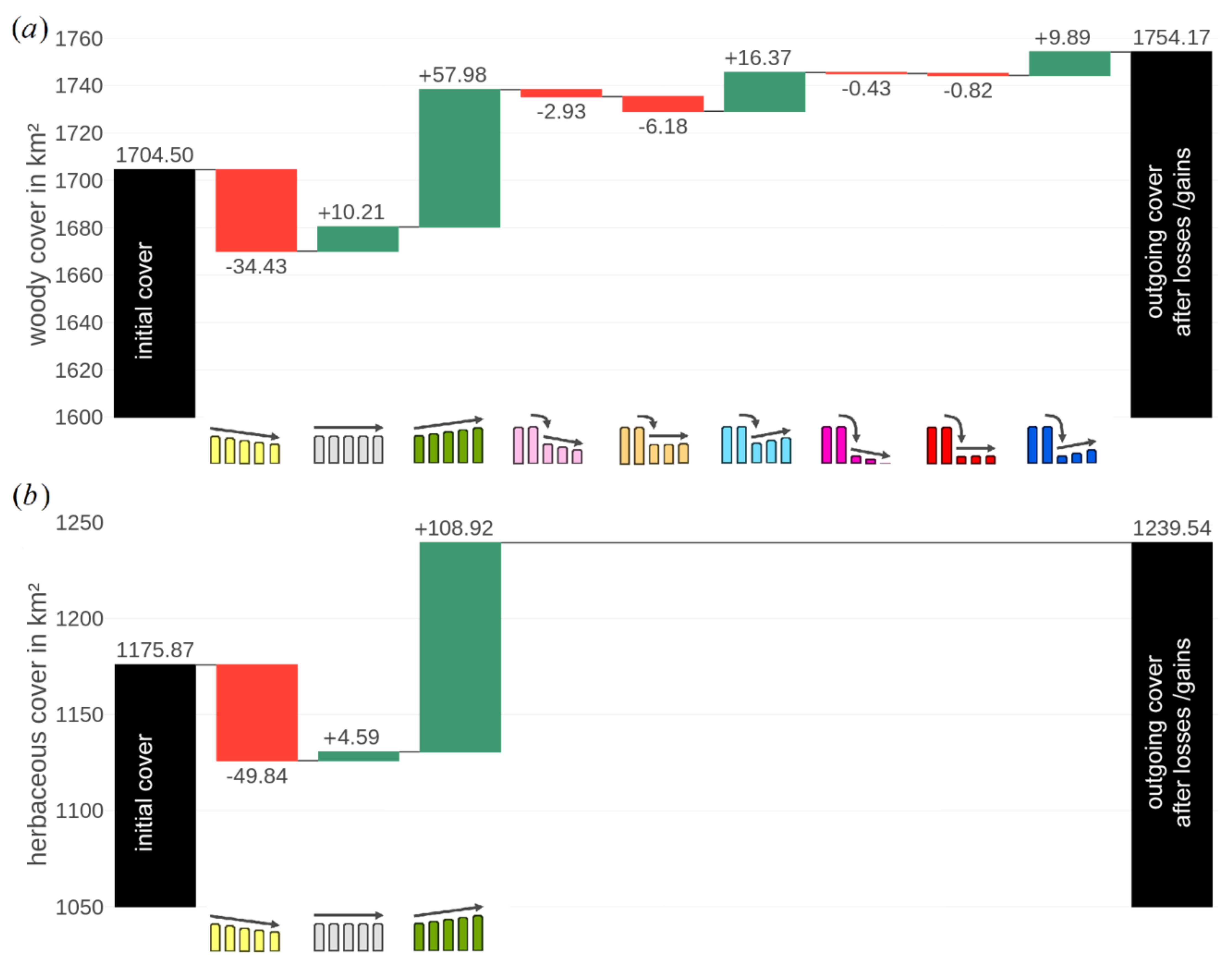
Next to the ecology-based syndrome classification, the absolute change in the cover is also important to consider as the previous assessment overestimated the actual vegetation cover that was lost or has accumulated. As an example, more biomass may be lost in productive areas than compared to high ranges with sparse vegetation cover. Thus, we additionally computed the absolute sub-pixel net cover change in m² over the complete period for each vegetation component (Figure 10). The net cover change varies regionally and is often pointing in opposite directions in the woody and herbaceous components (c.f. the rather stable total vegetation change in Figure 5b). As an example, a greening of the herbaceous layer in southern Crete is apparent while the higher ranges are more subject to an increase in woody vegetation. This decomposition is critical for carbon budgeting as, e.g., a loss in the woody vegetation is associated with a larger release of CO₂ as compared to the same amount of area lost in herbs (see e.g., [96] for biomass values). The total cover budget for all semi-natural areas in Crete (Figure 11) reveals that gains exceed losses for both herbaceous and woody components, thus resulting in a net gain of vegetation cover. This is in line with a general greening trend in the entire Mediterranean [97]. The gain is unanimously a result of the gradual long-term processes. The disturbances in the woody cover are fairly neutral overall (when considering the entire island): the cover lost through disturbances without regrowth is compensated by areas where the regrowth exceeds the magnitude of the disturbance.

5. Conclusions

We reproduced a past case study on land-use change induced land degradation in a Mediterranean ecosystem (“Vegetation Dynamics 1.0” [42]), which was conducted before the opening of the Landsat archive, and well before the remigration of European data holdings into the main data archive, thus inevitably being limited by data scarcity. Now, for the first time, the complete cross-calibrated data record over Europe was available and allowed to replicate this study with a state-of-the-art, data-driven, phenology-adaptive methodology based on the peak of season metric (“Vegetation Dynamics 2.0”). Following our findings, we conclude that trends derived from a Vegetation Dynamics 1.0 methodology are systematically prone to uncertainty due to a volatile timing of statically selected images relative to the spatially and inter-annually variable phenological cycle—sometimes close to peak vegetation cover, while other times close to minimal vegetation cover. This is especially critical if:

• a disturbance in the woody vegetation happened,
• a transition from/to woody/herbaceous vegetation took place, or
• inter-annual variability in seasonal herbaceous vegetation cover was high.

As expected, the majority of semi-natural areas in our study area were subject to at least one of these conditions. The employed Vegetation Dynamics 2.0 methodology yielded more robust results. Nonetheless, results also highlighted that:

• linear regression is too simplistic a tool to assess long-term vegetation cover change when stand-replacing disturbances in the woody vegetation cannot be ruled out, and that
• peak vegetation cover is not the optimal parameter to analyze.

A more nuanced and meaningful characterization could be achieved by further decomposing the total vegetation cover into woody and herbaceous components using the base level and seasonal amplitude metrics, respectively. The synoptic view on both change trajectories eventually allowed for:

• a more reliable interpretation of vegetation changes with respect to their trend direction and ecological meaning,
• to disentangle certain land-use change processes with opposite trajectories in the vegetation components that were unobservable when analyzing total vegetation cover,
• generating a long-term budget of net cover change, which revealed that vegetation cover of both components has increased at large, mainly due to gradual processes.

For the Earth observation-based assessment of long-term vegetation dynamics in semi-arid Mediterranean ecosystems, we conclude that static image selection study designs should be critically evaluated in the light of current data availability, analytical capabilities, and with regards to the ecosystem under investigation. This applies both to studies before the opening of the Landsat archive, and to contemporary papers implementing static selection. Although we only investigated one particular case study in the Mediterranean, we nevertheless postulate that similar findings would also apply to other cases and ecosystems. We recommend using all available data and take advantage of phenology-based approaches that remove the selection bias and hence reduce uncertainties in results.

References

1. Townshend, J.R.G.; Justice, C.O. Selecting the Spatial Resolution of Satellite Sensors Required for Global Monitoring of Land Transformations. Int. J. Remote Sens. 1988, 9, 187–236. [Google Scholar] [CrossRef]
2. Foley, J.A.; DeFries, R.; Asner, G.P.; Barford, C.; Bonan, G.; Carpenter, S.R.; Chapin, F.S.; Coe, M.T.; Daily, G.C.; Gibbs, H.K.; et al. Global Consequences of Land Use. Science 2005, 309, 570–574. [Google Scholar] [CrossRef] [PubMed] [Green Version]
3. Loveland, T.R.; Belward, A.S. The IGBP-DIS global 1km land cover data set, DISCover: First results. Int. J. Remote Sens. 1997, 18, 3289–3295. [Google Scholar] [CrossRef]
4. Defries, R.S.; Belward, A.S. Global and regional land cover characterization from satellite data: An introduction to the Special Issue. Int. J. Remote Sens. 2000, 21, 1083–1092. [Google Scholar] [CrossRef]
5. Belward, A.S.; Skøien, J.O. Who Launched What, When and Why; Trends in Global Land-Cover Observation Capacity from Civilian Earth Observation Satellites. ISPRS J. Photogramm. Remote Sens. 2015, 103, 115–128. [Google Scholar] [CrossRef]
6. Roy, D.P.; Wulder, M.A.; Loveland, T.R.; Woodcock, C.E.; Allen, R.G.; Anderson, M.C.; Helder, D.; Irons, J.R.; Johnson, D.M.; Kennedy, R.; et al. Landsat-8: Science and Product Vision for Terrestrial Global Change Research. Remote Sens. Environ. 2014, 145, 154–172. [Google Scholar] [CrossRef] [Green Version]
7. Cohen, W.B.; Goward, S.N. Landsat’s Role in Ecological Applications of Remote Sensing. BioScience 2004, 54, 535–545. [Google Scholar] [CrossRef]
8. Markham, B.L.; Helder, D.L. Forty-Year Calibrated Record of Earth-Reflected Radiance from Landsat: A Review. Remote Sens. Environ. 2012, 122, 30–40. [Google Scholar] [CrossRef] [Green Version]
9. Wulder, M.A.; White, J.C.; Loveland, T.R.; Woodcock, C.E.; Belward, A.S.; Cohen, W.B.; Fosnight, E.A.; Shaw, J.; Masek, J.G.; Roy, D.P. The global Landsat archive: Status, consolidation, and direction. Remote Sens. Environ. 2016, 185, 271–283. [Google Scholar] [CrossRef] [Green Version]
10. Masek, J.G.; Wulder, M.A.; Markham, B.; McCorkel, J.; Crawford, C.J.; Storey, J.; Jenstrom, D.T. Landsat 9: Empowering open science and applications through continuity. Remote Sens. Environ. 2020, 248, 111968. [Google Scholar] [CrossRef]
11. Wulder, M.A.; Loveland, T.R.; Roy, D.P.; Crawford, C.J.; Masek, J.G.; Woodcock, C.E.; Allen, R.G.; Anderson, M.C.; Belward, A.S.; Cohen, W.B.; et al. Current status of Landsat program, science, and applications. Remote Sens. Environ. 2019, 225, 127–147. [Google Scholar] [CrossRef]
12. Zhu, Z.; Wulder, M.A.; Roy, D.P.; Woodcock, C.E.; Hansen, M.C.; Radeloff, V.C.; Healey, S.P.; Schaaf, C.; Hostert, P.; Strobl, P.; et al. Benefits of the free and open Landsat data policy. Remote Sens. Environ. 2019, 224, 382–385. [Google Scholar] [CrossRef]
13. Wulder, M.A.; Masek, J.G.; Cohen, W.B.; Loveland, T.R.; Woodcock, C.E. Opening the Archive: How Free Data has Enabled the Science and Monitoring Promise of Landsat. Remote Sens. Environ. 2012, 122, 2–10. [Google Scholar] [CrossRef]
14. USGS. Landsat Thematic Mapper No-Payload Correction Data. Available online: https://www.usgs.gov/land-resources/nli/landsat/landsat-thematic-mapper-no-payload-correction-data (accessed on 31 October 2019).
15. Griffiths, P.; van der Linden, S.; Kuemmerle, T.; Hostert, P. A Pixel-Based Landsat Compositing Algorithm for Large Area Land Cover Mapping. IEEE J. Sel. Top. Appl. Earth Observ. Remote Sens. 2013, 6, 2088–2101. [Google Scholar] [CrossRef]
16. Suess, S.; van der Linden, S.; Okujeni, A.; Griffiths, P.; Leitão, P.J.; Schwieder, M.; Hostert, P. Characterizing 32 years of shrub cover dynamics in southern Portugal using annual Landsat composites and machine learning regression modeling. Remote Sens. Environ. 2018, 219, 353–364. [Google Scholar] [CrossRef]
17. Lebek, K.; Senf, C.; Frantz, D.; Monteiro, J.A.F.; Krueger, T. Interdependent effects of climate variability and forest cover change on streamflow dynamics: A case study in the Upper Umvoti River Basin, South Africa. Reg. Environ. Change 2019, 19, 1963–1971. [Google Scholar] [CrossRef]
18. Senf, C.; Laštovička, J.; Okujeni, A.; Heurich, M.; van der Linden, S. A generalized regression-based unmixing model for mapping forest cover fractions throughout three decades of Landsat data. Remote Sens. Environ. 2020, 240, 111691. [Google Scholar] [CrossRef]
19. Schneibel, A.; Stellmes, M.; Röder, A.; Frantz, D.; Kowalski, B.; Haß, E.; Hill, J. Assessment of spatio-temporal changes of smallholder cultivation patterns in the Angolan Miombo belt using segmentation of Landsat time series. Remote Sens. Environ. 2017, 195, 118–129. [Google Scholar] [CrossRef] [Green Version]
20. Griffiths, P.; Müller, D.; Kuemmerle, T.; Hostert, P. Agricultural Land Change in the Carpathian Ecoregion after the Breakdown of Socialism and Expansion of the European Union. Environ. Res. Lett. 2013, 8, 45024. [Google Scholar] [CrossRef]
21. DeFries, R.; Achard, F.; Brown, S.; Herold, M.; Murdiyarso, D.; Schlamadinger, B.; de Souza, C., Jr. Earth Observations for Estimating Greenhouse Gas Emissions from Deforestation in Developing Countries. Environ. Sci. Policy 2007, 10, 385–394. [Google Scholar] [CrossRef]
22. Frantz, D.; Röder, A.; Stellmes, M.; Hill, J. Phenology-adaptive pixel-based compositing using optical earth observation imagery. Remote Sens. Environ. 2017, 190, 331–347. [Google Scholar] [CrossRef] [Green Version]
23. Schneibel, A.; Frantz, D.; Röder, A.; Stellmes, M.; Fischer, K.; Hill, J. Using Annual Landsat Time Series for the Detection of Dry Forest Degradation Processes in South-Central Angola. Remote Sens. 2017, 9, 905. [Google Scholar] [CrossRef] [Green Version]
24. Zhu, Z.; Woodcock, C.E.; Holden, C.; Yang, Z. Generating synthetic Landsat images based on all available Landsat data: Predicting Landsat surface reflectance at any given time. Remote Sens. Environ. 2015, 162, 67–83. [Google Scholar] [CrossRef]
25. Zhu, Z.; Woodcock, C.E. Continuous Change Detection and Classification of Land Cover using all Available Landsat Data. Remote Sens. Environ. 2014, 144, 152–171. [Google Scholar] [CrossRef] [Green Version]
26. Verbesselt, J.; Hyndman, R.; Newnham, G.; Culvenor, D. Detecting trend and seasonal changes in satellite image time series. Remote Sens. Environ. 2010, 114, 106–115. [Google Scholar] [CrossRef]
27. Verbesselt, J.; Hyndman, R.; Zeileis, A.; Culvenor, D. Phenological change detection while accounting for abrupt and gradual trends in satellite image time series. Remote Sens. Environ. 2010, 114, 2970–2980. [Google Scholar] [CrossRef] [Green Version]
28. Zhang, J.; Shang, R.; Rittenhouse, C.; Witharana, C.; Zhu, Z. Evaluating the impacts of models, data density and irregularity on reconstructing and forecasting dense Landsat time series. Sci. Remote Sens. 2021, 4, 100023. [Google Scholar] [CrossRef]
29. Jönsson, P.; Cai, Z.; Melaas, E.; Friedl, M.A.; Eklundh, L. A Method for Robust Estimation of Vegetation Seasonality from Landsat and Sentinel-2 Time Series Data. Remote Sens. 2018, 10, 635. [Google Scholar] [CrossRef] [Green Version]
30. Jonsson, P.; Eklundh, L. Seasonality Extraction by Function Fitting to Time-Series of Satellite Sensor Data. IEEE Trans. Geosci. Remote Sens. 2002, 40, 1824–1832. [Google Scholar] [CrossRef]
31. Jönsson, P.; Eklundh, L. TIMESAT—A Program for Analyzing Time-Series of Satellite Sensor Data. Comput. Geosci. 2004, 30, 833–845. [Google Scholar] [CrossRef] [Green Version]
32. Bolton, D.K.; Gray, J.M.; Melaas, E.K.; Moon, M.; Eklundh, L.; Friedl, M.A. Continental-scale land surface phenology from harmonized Landsat 8 and Sentinel-2 imagery. Remote Sens. Environ. 2020, 240, 111685. [Google Scholar] [CrossRef]
33. Brooks, B.-G.J.; Lee, D.C.; Pomara, L.Y.; Hargrove, W.W. Monitoring Broadscale Vegetational Diversity and Change across North American Landscapes Using Land Surface Phenology. Forests 2020, 11, 606. [Google Scholar] [CrossRef]
34. Hill, J.; Stellmes, M.; Udelhoven, T.; Röder, A.; Sommer, S. Mediterranean desertification and land degradation: Mapping related land use change syndromes based on satellite observations. Glob. Planet. Change 2008, 64, 146–157. [Google Scholar] [CrossRef]
35. Stellmes, M.; Röder, A.; Udelhoven, T.; Hill, J. Mapping Syndromes of Land Change in Spain with Remote Sensing Time Series, Demographic and Climatic Data. Land Use Policy 2013, 30, 685–702. [Google Scholar] [CrossRef]
36. Tong, X.; Tian, F.; Brandt, M.; Liu, Y.; Zhang, W.; Fensholt, R. Trends of land surface phenology derived from passive microwave and optical remote sensing systems and associated drivers across the dry tropics 1992–2012. Remote Sens. Environ. 2019, 232, 111307. [Google Scholar] [CrossRef]
37. Hird, J.N.; Castilla, G.; McDermid, G.J.; Bueno, I.T. A Simple Transformation for Visualizing Non-seasonal Landscape Change from Dense Time Series of Satellite Data. IEEE J. Sel. Top. Appl. Earth Observ. Remote Sens. 2016, 9, 3372–3383. [Google Scholar] [CrossRef]
38. Kennedy, R.E.; Yang, Z.; Cohen, W.B. Detecting Trends in Forest Disturbance and Recovery using Yearly Landsat Time Series: 1. LandTrendr—Temporal Segmentation Algorithms. Remote Sens. Environ. 2010, 114, 2897–2910. [Google Scholar] [CrossRef]
39. Cohen, W.B.; Healey, S.P.; Yang, Z.; Stehman, S.V.; Brewer, C.K.; Brooks, E.B.; Gorelick, N.; Huang, C.; Hughes, M.J.; Kennedy, R.E.; et al. How Similar Are Forest Disturbance Maps Derived from Different Landsat Time Series Algorithms? Forests 2017, 8, 98. [Google Scholar] [CrossRef]
40. Healey, S.P.; Cohen, W.B.; Yang, Z.; Kenneth Brewer, C.; Brooks, E.B.; Gorelick, N.; Hernandez, A.J.; Huang, C.; Joseph Hughes, M.; Kennedy, R.E.; et al. Mapping forest change using stacked generalization: An ensemble approach. Remote Sens. Environ. 2018, 204, 717–728. [Google Scholar] [CrossRef]
41. National Academies of Sciences, Engineering, and Medicine. Reproducibility and Replicability in Science; The National Academies Press: Washington, DC, USA, 2019. [Google Scholar] [CrossRef]
42. Hostert, P.; Röder, A.; Hill, J. Coupling Spectral Unmixing and Trend Analysis for Monitoring of Long-Term Vegetation Dynamics in Mediterranean Rangelands. Remote Sens. Environ. 2003, 87, 183–197. [Google Scholar] [CrossRef]
43. Hostert, P.; Röder, A.; Hill, J.; Udelhoven, T.; Tsiourlis, G. Retrospective studies of grazing-induced land degradation: A case study in central Crete, Greece. Int. J. Remote Sens. 2003, 24, 4019–4034. [Google Scholar] [CrossRef]
44. Papanastasis, V. Traditional vs contemporary management of Mediterranean vegetation: The case of the island of Crete. J. Biol. Res. 2004, 1, 39–46. [Google Scholar]
45. Blondel, J. The ‘Design’ of Mediterranean Landscapes: A Millennial Story of Humans and Ecological Systems during the Historic Period. Hum. Ecol. 2006, 34, 713–729. [Google Scholar] [CrossRef]
46. Perevolotsky, A.; Seligman, N.a.G. Role of Grazing in Mediterranean Rangeland Ecosystems: Inversion of a paradigm. BioScience 1998, 48, 1007–1017. [Google Scholar] [CrossRef] [Green Version]
47. Lorent, H.; Sonnenschein, R.; Tsiourlis, G.M.; Hostert, P.; Lambin, E. Livestock Subsidies and Rangeland Degradation in Central Crete. Ecol. Soc. 2009, 14, 41. [Google Scholar] [CrossRef] [Green Version]
48. Kosmas, C.; Karamesouti, M.; Kounalaki, K.; Detsis, V.; Vassiliou, P.; Salvati, L. Land degradation and long-term changes in agro-pastoral systems: An empirical analysis of ecological resilience in Asteroussia—Crete (Greece). Catena 2016, 147, 196–204. [Google Scholar] [CrossRef]
49. Sonnenschein, R.; Kuemmerle, T.; Udelhoven, T.; Stellmes, M.; Hostert, P. Differences in Landsat-Based Trend Analyses in Drylands due to the Choice of Vegetation Estimate. Remote Sens. Environ. 2011, 115, 1408–1420. [Google Scholar] [CrossRef]
50. Hill, J.; Mehl, W. Geo- und radiometrische Aufbereitung multi- und hyperspektraler Daten zur Erzeugung langjähriger kalibrierter Zeitreihen. Photogramm. Fernerkund. Geoinf. 2003, 1, 7–14. [Google Scholar]
51. Hill, J.; Sturm, B. Radiometric Correction of Multitemporal Thematic Mapper Data for Use in Agricultural Land-Cover Classification and Vegetation Monitoring. Int. J. Remote Sens. 1991, 12, 1471–1491. [Google Scholar] [CrossRef]
52. Hill, J.; Mehl, W.; Radeloff, V. Improved forest mapping by combining corrections of atmospheric and topographic effects in landsat tm imagery. In Sensors and Environmental Applications of Remote Sensing; Askne, J., Ed.; Balkema: Rotterdam, The Netherlands, 1995; pp. 143–151. [Google Scholar]
53. Loveland, T.R.; Dwyer, J.L. Landsat: Building a Strong Future. Remote Sens. Environ. 2012, 122, 22–29. [Google Scholar] [CrossRef]
54. Woodcock, C.E.; Allen, R.; Anderson, M.; Belward, A.; Bindschadler, R.; Cohen, W.; Gao, F.; Goward, S.N.; Helder, D.; Helmer, E. Free Access to Landsat Imagery. Science 2008, 320, 1011. [Google Scholar] [CrossRef] [PubMed]
55. Potapov, P.; Turubanova, S.; Hansen, M.C. Regional-scale boreal forest cover and change mapping using Landsat data composites for European Russia. Remote Sens. Environ. 2011, 115, 548–561. [Google Scholar] [CrossRef]
56. Roy, D.P.; Ju, J.; Kline, K.; Scaramuzza, P.L.; Kovalskyy, V.; Hansen, M.; Loveland, T.R.; Vermote, E.; Zhang, C. Web-Enabled Landsat Data (WELD): Landsat ETM+ Composited Mosaics of the Conterminous United States. Remote Sens. Environ. 2010, 114, 35–49. [Google Scholar] [CrossRef]
57. Zhu, Z.; Woodcock, C.E. Object-Based Cloud and Cloud Shadow Detection in Landsat Imagery. Remote Sens. Environ. 2012, 118, 83–94. [Google Scholar] [CrossRef]
58. Yan, L.; Roy, D.P. Improving Landsat Multispectral Scanner (MSS) geolocation by least-squares-adjustment based time-series co-registration. Remote Sens. Environ. 2021, 252, 112181. [Google Scholar] [CrossRef]
59. Frantz, D. FORCE—Landsat + Sentinel-2 Analysis Ready Data and Beyond. Remote Sens. 2019, 11, 1124. [Google Scholar] [CrossRef] [Green Version]
60. Ernst, S.; Lymburner, L.; Sixsmith, J. Implications of Pixel Quality Flags on the Observation Density of a Continental Landsat Archive. Remote Sens. 2018, 10, 1570. [Google Scholar] [CrossRef] [Green Version]
61. Agou, V.D.; Varouchakis, E.A.; Hristopulos, D.T. Geostatistical analysis of precipitation in the island of Crete (Greece) based on a sparse monitoring network. Environ. Monit Assess. 2019, 191, 353. [Google Scholar] [CrossRef]
62. Frantz, D.; Stellmes, M. Water vapor database for atmospheric correction of Landsat imagery. IEEE Trans. Geosci. Remote Sens. 2018, 54, 3928–3943. [Google Scholar] [CrossRef]
63. Frantz, D.; Stellmes, M.; Hostert, P. A Global MODIS Water Vapor Database for the Operational Atmospheric Correction of Historic and Recent Landsat Imagery. Remote Sens. 2019, 11, 257. [Google Scholar] [CrossRef] [Green Version]
64. Wulder, M.A.; Coops, N.C.; Roy, D.P.; White, J.C.; Hermosilla, T. Land cover 2.0. Int. J. Remote Sens. 2018, 39, 4254–4284. [Google Scholar] [CrossRef] [Green Version]
65. R Core Team. R: A Language and Environment for Statistical Computing; R Foundation for Statistical Computing: Vienna, Austria, 2016; Available online: https://www.R-project.org/ (accessed on 18 September 2021).
66. Zhu, Z.; Wang, S.; Woodcock, C.E. Improvement and Expansion of the Fmask Algorithm: Cloud, Cloud Shadow, and Snow Detection for Landsats 4–7, 8, and Sentinel 2 Images. Remote Sens. Environ. 2015, 159, 269–277. [Google Scholar] [CrossRef]
67. Frantz, D.; Röder, A.; Udelhoven, T.; Schmidt, M. Enhancing the Detectability of Clouds and Their Shadows in Multitemporal Dryland Landsat Imagery: Extending Fmask. IEEE Geosci. Remote Sens. Lett. 2015, 12, 1242–1246. [Google Scholar] [CrossRef]
68. Frantz, D.; Röder, A.; Stellmes, M.; Hill, J. An Operational Radiometric Landsat Preprocessing Framework for Large-Area Time Series Applications. IEEE Trans. Geosci. Remote Sens. 2016, 54, 3928–3943. [Google Scholar] [CrossRef]
69. Zekoll, V.; Main-Knorn, M.; Louis, J.; Frantz, D.; Richter, R.; Pflug, B. Comparison of Masking Algorithms for Sentinel-2 Imagery. Remote Sens. 2021, 13, 137. [Google Scholar] [CrossRef]
70. Frantz, D. Generation of Higher Level Earth Observation Satellite Products for Regional Environmental Monitoring. Ph.D. Dissertation, Trier University, Trier, Germany, 2017. [Google Scholar]
71. Tanré, D.; Herman, M.; Deschamps, P.Y.; de Leffe, A. Atmospheric Modeling for Space Measurements of Ground Reflectances, Including Bidirectional Properties. Appl. Opt. 1979, 18, 3587–3594. [Google Scholar] [CrossRef]
72. Kaufman, Y.J.; Sendra, C. Algorithm for Automatic Atmospheric Corrections to Visible and Near-IR Satellite Imagery. Int. J. Remote Sens. 1988, 9, 1357–1381. [Google Scholar] [CrossRef]
73. Royer, A.; Charbonneau, L.; Teillet, P.M. Interannual Landsat-MSS Reflectance Variation in an Urbanized Temperate Zone. Remote Sens. Environ. 1988, 24, 423–446. [Google Scholar] [CrossRef]
74. Gao, B.-C.; Kaufman, Y.J. Water Vapor Retrievals using Moderate Resolution Imaging Spectroradiometer (MODIS) Near-Infrared Channels. J. Geophys. Res. Atmospheres 2003, 108, 3023. [Google Scholar] [CrossRef]
75. Doxani, G.; Vermote, E.; Roger, J.-C.; Gascon, F.; Adriaensen, S.; Frantz, D.; Hagolle, O.; Hollstein, A.; Kirches, G.; Li, F.; et al. Atmospheric Correction Inter-Comparison Exercise. Remote Sens. 2018, 10, 352. [Google Scholar] [CrossRef] [Green Version]
76. Buchner, J.; Yin, H.; Frantz, D.; Kuemmerle, T.; Askerov, E.; Bakuradze, T.; Bleyhl, B.; Elizbarashvili, N.; Komarova, A.; Lewińska, K.E.; et al. Land-cover change in the Caucasus Mountains since 1987 based on the topographic correction of multi-temporal Landsat composites. Remote Sens. Environ. 2020, 248, 111967. [Google Scholar] [CrossRef]
77. Bach, H. Die Bestimmung Hydrologischer und Landwirtschaftlicher Oberflächenparameter aus Hyperspektralen Fernerkundungsdaten; Geobuch-Verlag: Munich, Germany, 1995; Volume B 21. [Google Scholar]
78. Roy, D.P.; Zhang, H.K.; Ju, J.; Gomez-Dans, J.L.; Lewis, P.E.; Schaaf, C.B.; Sun, Q.; Li, J.; Huang, H.; Kovalskyy, V. A General Method to Normalize Landsat Reflectance Data to Nadir BRDF Adjusted Reflectance. Remote Sens. Environ. 2016, 176, 255–271. [Google Scholar] [CrossRef] [Green Version]
79. Lewis, A.; Lymburner, L.; Purss, M.B.J.; Brooke, B.; Evans, B.; Ip, A.; Dekker, A.G.; Irons, J.R.; Minchin, S.; Mueller, N.; et al. Rapid, high-resolution detection of environmental change over continental scales from satellite data—The Earth Observation Data Cube. Int. J. Digit. Earth 2016, 9, 106–111. [Google Scholar] [CrossRef]
80. Stellmes, M.; Udelhoven, T.; Röder, A.; Sonnenschein, R.; Hill, J. Dryland Observation at Local and Regional Scale—Comparison of Landsat TM/ETM+ and NOAA AVHRR Time Series. Remote Sens. Environ. 2010, 114, 2111–2125. [Google Scholar] [CrossRef]
81. Somers, B.; Asner, G.P.; Tits, L.; Coppin, P. Endmember variability in Spectral Mixture Analysis: A review. Remote Sens. Environ. 2011, 115, 1603–1616. [Google Scholar] [CrossRef]
82. Elmore, A.J.; Mustard, J.F.; Manning, S.J.; Lobell, D.B. Quantifying Vegetation Change in Semiarid Environments: Precision and Accuracy of Spectral Mixture Analysis and the Normalized Difference Vegetation Index. Remote Sens. Environ. 2000, 73, 87–102. [Google Scholar] [CrossRef]
83. Smith, M.O.; Ustin, S.L.; Adams, J.B.; Gillespie, A.R. Vegetation in deserts: I. A regional measure of abundance from multispectral images. Remote Sens. Environ. 1990, 31, 1–26. [Google Scholar] [CrossRef]
84. Bro, R.; De Jong, S. A fast non-negativity-constrained least squares algorithm. J. Chemom. 1997, 11, 393–401. [Google Scholar] [CrossRef]
85. Frantz, D.; Stellmes, M.; Röder, A.; Udelhoven, T.; Mader, S.; Hill, J. Improving the Spatial Resolution of Land Surface Phenology by Fusing Medium- and Coarse-Resolution Inputs. IEEE Trans. Geosci. Remote Sens. 2016, 54, 4153–4164. [Google Scholar] [CrossRef]
86. Vermote, E.; Justice, C.O.; Breon, F.M. Towards a Generalized Approach for Correction of the BRDF Effect in MODIS Directional Reflectances. Geosci. Remote Sens. IEEE Trans. 2009, 47, 898–908. [Google Scholar] [CrossRef]
87. Schwieder, M.; Leitão, P.J.; da Cunha Bustamante, M.M.; Ferreira, L.G.; Rabe, A.; Hostert, P. Mapping Brazilian savanna vegetation gradients with Landsat time series. Int. J. Appl. Earth Obs. Geoinf. 2016, 52, 361–370. [Google Scholar] [CrossRef]
88. Rufin, P.; Frantz, D.; Ernst, S.; Rabe, A.; Griffiths, P.; Özdoğan, M.; Hostert, P. Mapping Cropping Practices on a National Scale Using Intra-Annual Landsat Time Series Binning. Remote Sens. 2019, 11, 232. [Google Scholar] [CrossRef] [Green Version]
89. Tulleken, H. Poisson Disk Sampling. Dev. Mag. 2008, 21, 21–25. [Google Scholar]
90. Muir, J.; Schmidt, M.; Tindall, D.; Trevithick, R.; Scarth, P.; Stewart, J. Field Measurement of Fractional Ground Cover: A Technical Handbook Supporting Ground Cover Monitoring for Australia; ACT ABARES: Canberra, Australia, 2011. [Google Scholar]
91. Danaher, T.; Scarth, P.; Armston, J.; Collett, L.; Kitchen, J.; Gillingham, S. Remote sensing of tree-grass systems: The eastern australian woodlands. In Ecosystem Function in Savannas: Measurement and Modeling at Landscape to Global Scales; Hill, M.J., Hanan, N.P., Eds.; CRC Press: Boca Raton, FL, USA, 2010; pp. 175–194. [Google Scholar] [CrossRef]
92. Bunker, B.E.; Tullis, J.A.; Cothren, J.D.; Casana, J.; Aly, M.H. Object-based Dimensionality Reduction in Land Surface Phenology Classification. AIMS Geosci. 2016, 2, 302–328. [Google Scholar] [CrossRef]
93. Ives, A.R.; Zhu, L.; Wang, F.; Zhu, J.; Morrow, C.J.; Radeloff, V.C. Statistical inference for trends in spatiotemporal data. Remote Sens. Environ. 2021, 266, 112678. [Google Scholar] [CrossRef]
94. Röder, A.; Udelhoven, T.; Hill, J.; del Barrio, G.; Tsiourlis, G. Trend Analysis of Landsat-TM and -ETM+ Imagery to Monitor Grazing Impact in a Rangeland Ecosystem in Northern Greece. Remote Sens. Environ. 2008, 112, 2863–2875. [Google Scholar] [CrossRef]
95. Pulina, G.; Cappio-Borlino, A.; D’Angelo, M.; Francesconi, A. Grazing in Mediterranean ecosystems: A complex approach as addressed in the EU Medalus project. In Proceedings of the International Workshop Ecological Basis of Livestock Grazing in Mediterranean Ecosystems, Thessaloniki, Greece, 23–25 October 1997; pp. 173–188. [Google Scholar]
96. Moustakas, A.; Sakkos, K.; Wiegand, K.; Ward, D.; Meyer, K.M.; Eisinger, D. Are savannas patch-dynamic systems? A landscape model. Ecol. Model. 2009, 220, 3576–3588. [Google Scholar] [CrossRef]
97. Pausas, J.G.; Millán, M.M. Greening and Browning in a Climate Change Hotspot: The Mediterranean Basin. BioScience 2019, 69, 143–151. [Google Scholar] [CrossRef] [Green Version]
Figure 1. (a) Number of clear-sky Landsats 4–7 observations for 1984–2006 (b) and Digital Elevation Model.
Remotesensing 14 00597 g001
Figure 2. Workflow. Black boxes represent data; white boxes represent processing steps. The dates in the paper symbol represent literature-sourced dates used for generating pixel-based composites.
Remotesensing 14 00597 g002
Figure 3. Fractional cover time series for two selected pixels. (a,b) Mixture of rock, grass, and shrub surfaces (35.36°N, 24.92°E); (c,d) mixture of rock and grass surfaces, with a higher share of woody vegetation before disturbance (35.29°N, 24.96°E). (a,c) Time-series plotted as a temporal sequence; (b,d) time series plotted in polar space; the grey isolines match the 10% fraction increments shown as horizontal lines in (a,c). The color-coding is consistent between related plots and shows the interpolated time series. Green circles represent the value of peak of season (VPS) metric; white circles represent the beginning/end of the phenological years θ s ¯ ; the lines in between represent the value of base-level (VBL) metric; the arrows represent the value of seasonal amplitude (VSA) metric.
Remotesensing 14 00597 g003
Figure 4. Expert-driven decision tree for classifying change and trend parameters for an information-enriched long-term vegetation change assessment.
Remotesensing 14 00597 g004
Figure 5. Cover change for the Vegetation Dynamics 1.0 (a) and Vegetation Dynamics 2.0 (b) analyses over the study period 1984–2006. White areas are non-natural areas or above 1500 m a.s.l., which were out of scope of this study.
Remotesensing 14 00597 g005
Figure 6. Zoom on Psiloritis area, i.e., study area of [42]. (a,b) As in Figure 5. (c) Delta cover change (ΔCC), i.e., Figure 6a,b. The colors read as follows: blue to red colors represent a cover loss in both methods, while blue (red) indicates less (more) loss in the Vegetation Dynamics 2.0 methodology; green to orange colors represent a cover gain in both methods, while green (orange) indicates a larger (smaller) gain in the Vegetation Dynamics 2.0 methodology. Pink and cyan represent areas with different change directions, where pink indicates a loss (gain) in Vegetation Dynamics 2.0 (1.0) and cyan indicates a gain (loss) in Vegetation Dynamics 2.0 (1.0). The point signatures in (c) refer to the pixels shown in Figure 7. White areas are non-natural areas or above 1500 m a.s.l., which were out of scope of this study.
Remotesensing 14 00597 g006
Figure 7. Representative time series for the different delta cover change types in Figure 6. Color coding as in Figure 3. Green circles represent the value of peak of season (VPS) metric (Vegetation Dynamics 2.0); white circles are the statically selected images from Vegetation Dynamics 1.0. Regression lines and cover change for both methods are shown. Subplots (af) are representative pixels that are referred to in the text below. The point locations are shown in Figure 6c.
Remotesensing 14 00597 g007
Figure 8. Long-term change of vegetation components over the study period 1984–2006. (a) RGB representation of the major vegetation components for 1985; stretched from 0–100%; an animation for the complete time series is available in the supplemental material. (b,c) Syndrome-based labeling of land-use change classes for woody and herbaceous vegetation trajectories, respectively. White areas are non-natural areas or above 1500 m a.s.l., which were out of scope of this study.
Remotesensing 14 00597 g008
Figure 9. Combinations of herbaceous and woody vegetation cover change over the study period 1984–2006. The width of the links is related to the area under the respective change combination. Numeric data in Table 5.
Remotesensing 14 00597 g009
Figure 10. Net cover change for the woody (a) and herbaceous vegetation (b) over the study period 1984–2006. Net cover change is in m2. The complete removal of a completely vegetated pixel (e.g., a dense forest) would result in a loss of −900 m2. White areas are non-natural areas or above 1500 m a.s.l., which were out of scope of this study.
Remotesensing 14 00597 g010
Figure 11. Vegetation cover bookkeeping for all semi-natural areas in Crete. (a) Woody vegetation; (b) herbaceous vegetation. The gains/losses of the individual vegetation dynamics syndromes are subsequently booked on the initial vegetation cover (1984), thus resulting in the outgoing vegetation cover (2006).
Remotesensing 14 00597 g011