Transformer Neural Network for Weed and Crop Classification of High Resolution UAV Images

Abstract

Monitoring crops and weeds is a major challenge in agriculture and food production today. Weeds compete directly with crops for moisture, nutrients, and sunlight. They therefore have a significant negative impact on crop yield if not sufficiently controlled. Weed detection and mapping is an essential step in weed control. Many existing research studies recognize the importance of remote sensing systems and machine learning algorithms in weed management. Deep learning approaches have shown good performance in many agriculture-related remote sensing tasks, such as plant classification, disease detection, etc. However, despite the success of these approaches, they still face many challenges such as high computation cost, the need of large labelled datasets, intra-class discrimination (in growing phase weeds and crops share many attributes similarity as color, texture, and shape), etc. This paper aims to show that the attention-based deep network is a promising approach to address the forementioned problems, in the context of weeds and crops recognition with drone system. The specific objective of this study was to investigate visual transformers (ViT) and apply them to plant classification in Unmanned Aerial Vehicles (UAV) images. Data were collected using a high-resolution camera mounted on a UAV, which was deployed in beet, parsley and spinach fields. The acquired data were augmented to build larger dataset, since ViT requires large sample sets for better performance, we also adopted the transfer learning strategy. Experiments were set out to assess the effect of training and validation dataset size, as well as the effect of increasing the test set while reducing the training set. The results show that with a small labeled training dataset, the ViT models outperform state-of-the-art models such as EfficientNet and ResNet. The results of this study are promising and show the potential of ViT to be applied to a wide range of remote sensing image analysis tasks.

1. Introduction

Agriculture is at the heart of scientific evolution and innovation to face major challenges for achieving high yield production while protecting plants growth and quality to meet the anticipated demands on the market [1]. However, a major problem arising in modern agriculture is the excessive use of chemicals to boost the production yield and to get rid of unwanted plants such as weeds from the field [2]. Weeds are generally considered harmful to agricultural production [3]. They compete directly with crop plants for water, nutrients and sunlight [4]. Herbicides are often used in large quantities by spraying all over agricultural fields which has, however, shown various concerns like air, water and soil pollution and promoting weed resistance to such chemicals [2]. If the rate of usage of herbicides remains the same, in the near future, weeds will become fully resistant to these products and eventually destroy the harvest [5]. This is why weed and crop control management is becoming an essential field of research nowadays [6].

Automated crop monitoring system is a practical solution that can be beneficial both economically and environmentally. Such a system can reduce labour costs by making use of robots to remove weeds and hence minimising the use of herbicides [7]. The foremost step to an automatic weed control system is the detection and mapping of weeds on the field which can be a challenging part as weeds and crop plants often have similar colours, textures, and shapes [4]. The use of Unmanned Aerial Vehicles (UAVs) has proved significant results for mapping weed density across a field by collecting RGB images ([8,9,10,11,12]) or multispectral images ([13,14,15,16,17]) covering the whole field. As UAVs fly over the field at an elevated altitude, the images captured cover a large ground surface area and these large images can be split into smaller tiles to facilitate their processing ([18,19,20]) before feeding them to learning algorithms to identify and classify a weed from a crop plant.

In the agricultural domain, the main approach to plant detection is to first extract vegetation from the image background using segmentation and then distinguish crops from the weeds [21]. Common segmentation approaches use multispectral information to separate the vegetation from the background (soil and residuals) [22]. However, weeds and crops are difficult to distinguish from one another even while using spectral information because of their strong similarities [23]. This point has also been highlighted in [6], in which the authors reported the importance of using both spectral and spatial features to identify weeds in crops. In traditional machine learning approaches, features are handcrafted and then algorithms like support vector machines (SVM) are used to generate discriminative models. For example, the authors in [24,25] used this method to detect weeds in potato fields. Literature reviews of this type of approach for weed detection can be found in [26,27].

Classical machine learning approaches depend on feature engineering, where one has to design feature extractors, which generally performs well on small databases but fails on larger and varied data. In contrast, deep learning (DL) approaches rely on learning feature extractors and have shown much better performance compared to traditional methods. Therefore, DL becames an essential approach in image classification, object detection and recognition [28,29] notably in the agricultural domain [30]. DL models with architectures based on Convolutional Neural Network (CNN), have been applied to various domains as they yield high accuracy for image classification and object detection tasks [31,32,33]. CNN uses convolutional filters on an image to extract important features to understand the object of interest in an image with the help of convolutional operations covering key properties such as local connection, parameters (weight) sharing and translation equivariance [28,34]. Numerous papers covering weed detection or classification make use of CNN-based model structures [35,36,37] such as AlexNet [32], VGG-19, VGG-16 [38], GoogLeNet [39], ResNet-50, ResNet-101 [33] and Inception-v3 [40].

On the other hand, attention mechanism has seen a rapid development particularly in natural language processing (NLP) [41] and has shown impressive performance gains when compared to previous generation of models [42]. In vision applications, the use of attention mechanism has been much more limited, due to the high computational cost as the number of pixels in an image is much larger than the number of units of words in NLP applications. This makes it impossible to apply standard attention models to images. A recent survey of applications of transformer networks in computer vision can be found in [43]. The recently proposed vision transformer (ViT) appears to be a major step towards adopting transformer-attention models for computer vision tasks [44]. Where image patches are considered as units of information for training, whereas CNN-based methods operate on image pixel level. ViT incorporates image patches into a shared space and learns the relation between these patches using self-attention modules. Given massive amounts of training data and computational resources, ViT was shown to surpass CNNs in image classification accuracy [44]. Vision transformer models have not been explored yet for the task of weeds and crops classification of high resolution UAV images. To our best knowledge, there is no study that has examined their potential for such a task.

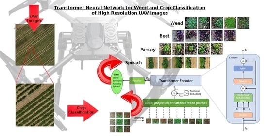
In this paper, we propose a methodology to automatically recognize weeds and crops in drone images using the vision transformer approach. We set up an acquisition system with a drone and a high resolution camera. The images were captured in real-world conditions on plots of different crops: red leaf beet, green leaf beet, parsley and spinach. The main objective was to study the paradigm of transformers architectures for specific tasks such as plant recognition in UAV images, where labeled data are not available in large quantities. Data augmentation and transfer learning were used as a strategy to fill the gap of labeled data. To evaluate the performance of the self-attention mechanism via vision transformers, we fluctuated the proportions of data used for training and for testing within cross-validation scheem. The contributions are summarized in the following points:

• Low-altitude aerial imagery based on UAVs and self-attention algorithms for crop management.
• First study to explore the potential of transformers for classification of weed and crop images.
• Evaluation of the generalization capabilities of deep learning algorithms with regard to train set reduction, in crop plants classification task.

The rest of the paper is organised as follows: Section 2 presents the materials and methods used as well as a brief description of the self-attention mechanism and the vision transformer model architecture. The experimental results and analysis are presented in Section 3 and Section 4. We discuss the results in Section 5. Section 6 summarizes our study and provides some perspectives.

2. Materials and Methods

This section outlines the acquisition, preparation and labeling of the dataset acquired using a high resolution camera mounted on a UAV, and describes both: the self-attention paradigm and the vision transformer model architecture.

2.1. Image Collection and Annotation

The study area is composed of crop fields of beet, parsley and spinach located in the Centre-Val de Loire Region, in France. It is a highly agricultural region as it presents many pedo-climatic advantages: the region has limited rainfall and clay-limestone soils with good filtering capacity. Irrigation is also offered on 95% of the plots, enabling controlled water conditions.

To survey the study area, a “Starfury”, Pilgrim UAV was equipped with a Sony ILCE-7R, 36 mega pixel camera as shown in Figure 1. The camera is mounted to the drone using a 3-axis stabilized brushless gimbals in order to keep the camera axis stable even during strong winds. The drone flight altitude was respectively of 30 m for the beet field and 20 m for the parsley and spinach fields. These altitudes where selected to minimize drone flight times while maintaining sufficient image quality. The beet plants being more developed, a higher altitude was selected. The aerial image acquisitions of the 3 fields were also conducted at different times depending of the weed levels reported by ground field experts. Acquiring images over multiple days resulted in adding variability in the images, as the beet field was flown by a light morning fog and the parsley and spinach fields under sunnier weather conditions.

The drone followed a specific flight plan and the camera captured RGB images at regular intervals as shown in Figure 2 and Figure 3. The images captured have respectively a minimum longitudinal and lateral overlapping of 70% and 50–60% depending on the fields vegetation coverage and homogeneity, assuring a better and complete coverage of the whole field of 4 ha (40,000 m${}^2$) and improving the accuracy of the orthorectified image of the field.

The data were manually processed using the annotation tool LabelImg (https://github.com/tzutalin/labelImg, accessed on 7 September 2021) on the tiles of the orthorectified image. Weeds and crops were annotated using bounding boxes, which may have various sizes and contain a portion of the object of interest. We extract the crop and weed image patches from the bounding boxes. Then, the image patches are resized to 64 × 64 pixels. This image size was chosen because the bounding box dimensions were centered around 64 × 64 pixels, which may be proportionally related to the flight height of the UAV and the size of the crops observed in the study fields. Resizing the patches to the average bounding box dimensions also limits width and height distortions in the input images. We divided the crop and weed labels into 5 classes as shown in Figure 4. We have a class for each of the studied crops, an overall weed class, and an off-type green leaf beet class.

2.2. Image Preprocessing

Manual image labeling being a very time consuming task which implying huge labor costs, therefore, we limited the manual labeling to 4000 samples for each crop and weed classes. Off-type green leaf beet is not as well represented as the other 4 classes, with only 653 labeled samples. In order to tackle this class imbalance, we upsampled four times the off-type beet class up to 3265 samples, by performing random flips and rotations. Resulting in a dataset distribution of 16.9% of off-type beet plants, and equally 20.8% images for the four other classes as presented in

Table 1. Class Distribution.

Class	Number
Weed	4000
Beet	4000
Off-type Beet	3265
Parsley	4000
Spinach	4000

, for a total of 19,265 images of size 64 × 64.

Images have been rescaled to 0–1 range and then normalized by scaling the pixels values to have a zero mean and unit variance before being divided into training, validation and testing sets.

During the training phase, we employed data augmentation strategies to enrich the datasets as it plays an important role in deep learning [45]. The augmentations applied can be summed up as random resized crop, colour jitters and rand augments [46]. This technique is implemented using Keras ImageDataGenerator, generating augmented images on the fly.Data augmentations were used to help improve the robustness of the model and generalisation capabilities by expanding the training dataset and simulate real-world agricultural scenarios as they can vary a lot depending on the soil, environment, season and climate conditions.

2.3. ViT Self-Attention

The attention mechanism is becoming a key concept in the deep learning field [47]. Attention was inspired by the human perception process where the human tends to focus on parts of information, ignoring other perceptible parts of information at the same time. The attention mechanism has had a profound impact on the field of natural language processing, where the goal was to focus on a subset of important words. The self-attention paradigm has emerged from the concepts attention showing improvement in the performance of deep networks [42].

Let us denote a sequence of n entities (${\mathbf{x}}_{\mathbf{1}},{\mathbf{x}}_{\mathbf{2}},\cdots ,{\mathbf{x}}_{\mathbf{n}}$) by $X\in {\mathbb{R}}^{n\times d}$, where d is the embedding dimension to represent each entity. The goal of self-attention is to capture the interaction amongst all n entities by encoding each entity in terms of the global contextual information. This is done by defining three learnable weight matrices, Queries ($W^Q\in {\mathbb{R}}^{n\times d_q}$), Keys ($W^K\in {\mathbb{R}}^{n\times d_k}$) and Values ($W^V\in {\mathbb{R}}^{n\times d_v}$). The input sequence X is first projected onto these weight matrices to get $Q=X{W}^Q,K=X{W}^K$ and $V=X{W}^V$.

The attention matrix $A\in {\mathbb{R}}^{n\times d_v}$ indicates a score between N queries Q and $K^T$ keys representing which part of the input sequence to focus on.

$$A(Q,K)=\sigma \left(Q{K}^T\right)$$

(1)

where $\sigma$ is an activation function, usually $softmax\left(\right)$. To capture the relations among the input sequence, the values V are weighted by the scores from Equation (1). Resulting in [44],

$$\begin{array}{c}\hfill SelfAttention(Q,K,V)=A(Q,K)·V\\ \hfill \Rightarrow SelfAttention(Q,k,V)=softmax\left(\frac{Q{K}^T}{\sqrt{d_k}}\right)·V\end{array}$$

(2)

where $d_k$ is dimension of the input queries.

If each pixel in a feature map is regarded as a random variable and the covariances are calculated, the value of each predicted pixel can be enhanced or weakened based on its similarity to other pixels in the image. The mechanism of employing similar pixels in training and prediction and ignoring dissimilar pixels is called the self-attention mechanism. It helps to relate different positions of a single sequence of image patches in order to gain a more vivid representation of the whole image [48].

The transformer network is an extension of the attention mechanism from Equation (2) based on the Multi-Head Attention operation. It is based on running k self-attention operations, called “heads”, in parallel, and project their concatenated outputs [42]. This helps the transformer jointly attend to different information derived from each head. The output matrix is obtained by the concatenation of each attention heads and a dot product with the weight $W^O$. Hence, generating the output of the multi-headed attention layer. The overall operation is summarised by the equations below [42].

$$\begin{array}{c}\hfill MultiHead(Q,K,V)=Concat(hea{d}_1,...,hea{d}_h)W^O\\ \hfill wherehea{d}_i=Attention(Q{W}_i^Q,K{W}_i^K,V{W}_i^V)\end{array}$$

(3)

where $W_i^Q,W_i^K,W_i^V$ are weight matrices for queries, keys and values respectively and $W^O\in {\mathbb{R}}^{h{d}_v\times d_{model}}$.

By using the self-attention mechanism, global reference can be realised during the training and prediction of models. This helps in reducing by a considerable amount training time of the model to achieve high accuracy [44]. The self-attention mechanism is an integral component of transformers, which explicitly models the interactions between all entities of a sequence for structured prediction tasks. Basically, a self-attention layer updates each component of a sequence by aggregating global information from the complete input sequence. While, the convolution layers’ receptive field is a fixed $K\times K$ neighbourhood grid, the self-attention’s receptive field is the full image. The self-attention mechanism increases the receptive field compared to the CNN without adding computational cost associated with very large kernel sizes [49]. Furthermore, self-attention is invariant to permutations and changes in the number of input points. As a result, it can easily operate on irregular inputs as opposed to standard convolution that requires grid structures [43].

Average attention weights of all heads mean heads across layers and the head in the same layer. Basically, the area has every attention in the transformer which is called attention pattern or attention matrix. When the patch of the weed image is passed through the transformer, it will generate the attention weight matrix for the image patches (see Figure 5). For example, when patch 1 is passed through the transformer, self-attention will calculate how much attention should pay to others (patch 2, patch 3, ...). In addition, every head will have one attention pattern as shown in Figure 6 and finally, they will sum up all attention patterns (all heads). We can observe that the model tries to identify the object (weed) on the image and tries to focus its attention on it (as it stands out from the background).

An attention mechanism is applied to selectively give more importance to some of the locations of the image compared to others, for generating caption(s) corresponding to the image. In addition, consequently, this helps to focus on the main differences between weeds and crops in an images and improves the learning of the model to identify the contrasts between these plants. This mechanism also helps the model to learn features faster, and eventually decreases the training cost [44].

2.4. Vision Transformers

Transformer models were major headway in NLP. They became the standard for modern NLP tasks and they brought spectacular performance yields when compared to the previous generation of state-of-the-art models [42]. Recently, it was reviewed and introduced to computer vision and image classification aiming to show that this reliance on CNNs is not necessary anymore in object detection or image classification and a pure transformer applied directly to sequences of image patches can perform very well on image classification tasks [44].

Figure 7 presents the architecture of the vision transformer used in this paper for weed and crop classification. It is based on the first developed ViT model by Dosovitskiy et al. [44]. The model architecture consists of 7 main steps. Firstly, the input image is split into smaller fixed-size patches. Then each patch is flattened into a 1-D vector. The input sequence consists of the flattened vector (2D to 1D) of pixel values from a patch of size 16 × 16.

For an input image,

$$\left(x\right)\in {\mathbb{R}}^{H\times W\times C}$$

(4)

and patch size P, N image patches are created

$${\left(x\right)}_P\in {\mathbb{R}}^{N\times P\times P\times C}$$

(5)

with

$$N=\frac{HW}{P\times P}$$

(6)

where N is the sequence length (token) similar to the words of a sentence, $(H,W)$ is the resolution of the original image and C is the number of channels [44].

Afterwards, each flattened element is then fed into a linear projection layer that will produce what is called the “patch embedding”. There is one single matrix, represented as ‘E’ (embedding) used for the linear projection. A single patch is taken and first unrolled into a linear vector as shown in Figure 8. This vector is then multiplied with the embedding matrix E. The final result is then fed to the transformer, along with the positional embedding. In the 4^th phase, the position embeddings are linearly added to the sequence of image patches so that the images can retain their positional information. It injects information about the relative or absolute position of the image patches in the sequence. The next step is to attach an extra learnable (class) embedding to the sequence according to the position of the image patch. This class embedding is used to predict the class of the input image after being updated by self-attention. Finally, the classification is performed by stacking a multilayer perceptron (MLP) head on top of the transformer, at the position of the extra learnable embedding that has been added to the sequence.

3. Performance Evaluation

We made use of recent implementations of ViT-B32 and ViT-B16 models as well as EfficientNet and ResNet models. The algorithms were built on top of a Tensorflow 2.4.1 and Keras 2.4.3 frameworks using Python 3.6.9. To run and evaluate our methods, we used the following hardware; an Intel Xeon(R) CPU E5-1620 v4 3.50 GHz x 8 processor (CPU) with 16 GB of RAM, and a graphics processing unit (GPU) NVIDIA Quadro M2000 with an internal RAM of 4 GB under the Linux operating system Ubuntu 18.04 LTS (64 bits).

All models were trained using the same parameters in order to have an unbiased and reliable comparison between their performance. The initial learning rate was set to 0.0001 with a reducing factor of 0.2. The batch size was set to 8 and the models were trained for 100 epochs with an early stopping after a wait of 10 epochs without better scores. The models used, ViT-B16, ViT-B32, EfficientNet B0, EfficientNet B1 and ResNet 50 were loaded from the keras library with pre-trained weights of “ImageNet”.

We limited the comparison of the ViT Based models with ResNet and EfficientNet CNN architectures as they are widely used CNN architectures and have been applied to various study domains. More specifically, the ResNet architecture [33] was the first CNN architecture introducing residual blocks. Where the residual blocks use skip connections between layers providing alternative paths for the gradient backpropagation, resulting in improving accuracy. We selected the ResNet-50 version for the residual architecture using 3-layer building blocks which yields better results compared to 2-layer building blocks as used in ResNet-34. The second CNN architecture considered is the EfficientNet architecture [50], the particularity of the EfficientNet neural network family is that is has highly optimised parameters and yields equivalent or higher Top-1 results depending on the version of the network used.

3.1. Cross-Validation

The experiments have been carried out using the cross-validation technique to ensure the integrity and accuracy of the models. Cross-validation is a widely used technique for assessing models as the performance evaluation is carried out on unseen test data [51], the method also presents the advantage of being a low bias resampling method [52].

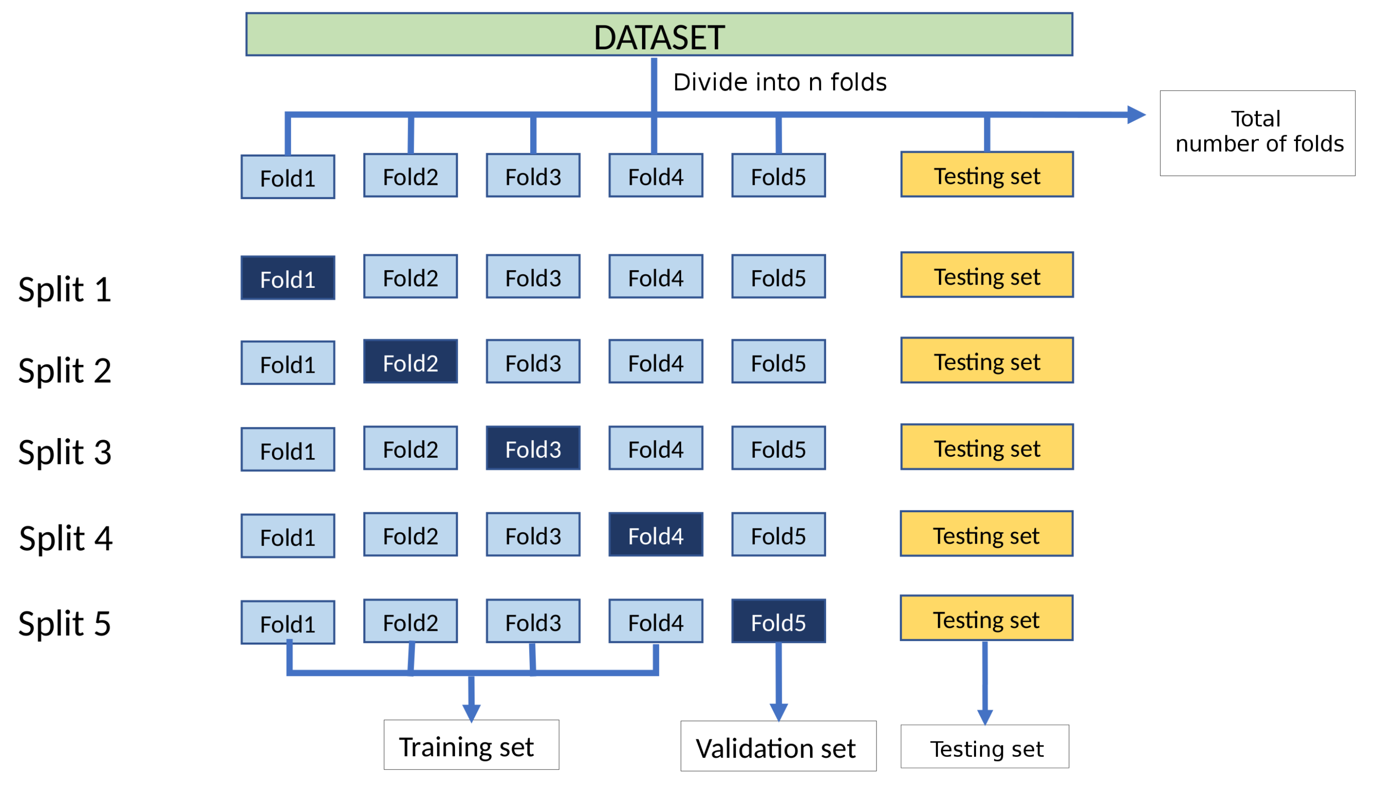
As our dataset classes are not perfectly balanced we applied stratified K-Fold. By applying stratification, each randomly sampled fold will have an equal class distribution in respect to the total dataset distribution. From these folds we then test the performance of the models using the k-fold cross-validation leaving k folds as validation set.

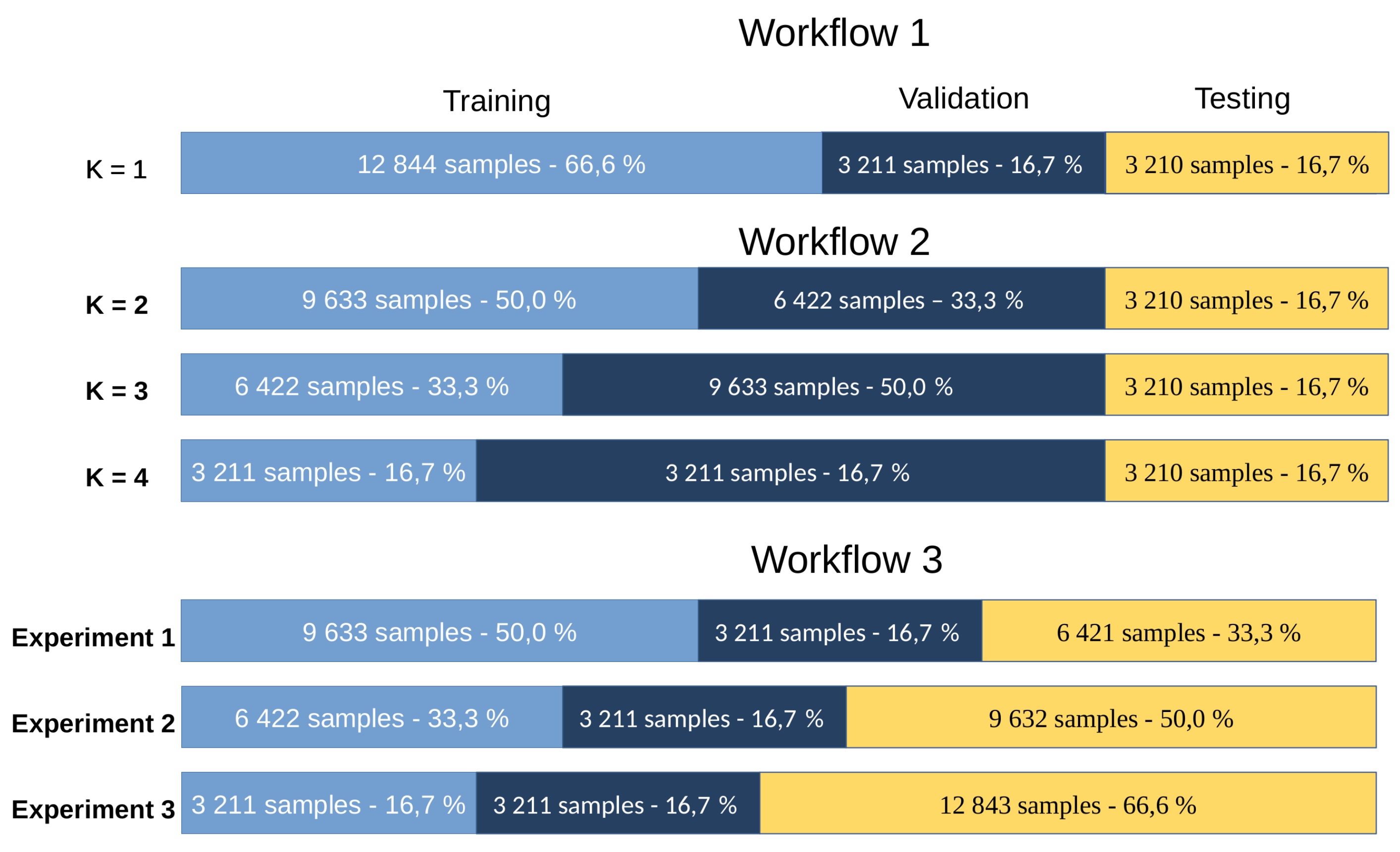
To assess the performance of ViT models with respect to the selected CNN architectures, we performed 3 workflows. First, we performed cross-validation with one validation set (k = 1) to maximize the size of the training dataset and evaluate the performance at a fixed test fold (see Figure 9). Second, we decreased the number of training folds and increased the size of the validation set while keeping the same test fold. Finally, we reduced the number of training folds while maintaining a single validation fold (k = 1) and increasing the size of the test set, to evaluate the predictive performance of the models when trained on small data sets.

Using the stratified five-folds cross-validation leaving k folds as validation set (where $1\le k\le 4$), Figure 10 shows how the dataset is splitted with $n=5$ and $k=2$ where n represents the total number of cross-validation folds, resulting in the training of 10 models. Increasing the value of k, decreases the number of folds used for training and thus forces the model to train on a smaller dataset. This helps to evaluate how well the models perform on reduced training datasets and their capacities to extract features from fewer image samples. The number of combination (splits) of the train-validation is as follows:

$$C_k^n=\frac{n!}{k!(n-k)!}$$

(7)

where n is the number of folders and k is the number of validation folds.

For the third workflow, we conducted three experiments. The number of testing images is increased for each experiment, consequently decreasing the number of training images. In experiment 1, the dataset was split into 9633 training and 6421 testing images. In experiment 2, the dataset was divided into 6422 training and 9633 testing images. Experiment 3 contains only 3211 training images for 12,843 testing images. Each set up of experiments is then trained using the cross-validation technique (see Figure 11).

3.2. Evaluation Metrics

In the collected dataset, each image has been manually classified into one of the categories: weeds, off-type beet (green leaves beet), beet (red leaves), parsley or spinach, called ground-truth data. By running the classifiers on a test set, we obtained a label for each testing image, resulting in the predicted classes. The classification performance is measured by evaluating the relevance between the ground-truth labels and the predicted ones resulting in classification probabilities of true positives (TP), false positives (FP) and false negatives (FN). We then calculate a recall measure representing how well a model correctly predicts all the ground-truth classes and a precision representing the ratio of how many of the positive predictions were correct relative to all the positive predictions.

$$\begin{array}{c}\hfill Precision=\frac{TP}{TP+FP}\\ \hfill Recall=\frac{TP}{TP+FN}\end{array}$$

(8)

The metrics used in the evaluation procedure were the precision, recall and F1-Score [53], the latter being the weighted average of precision and recall, hence considering both false positive and false negatives. Comparison studies have shown that these metrics are relevant for evaluation of classification model performance [54].

These metrics were also selected as in opposition to accuracy, they are invariant to class distribution. This invariance property is due to the consideration of only TP and not TN predictions in the computation of precision and recall [55]. Not taking TNs into account can sometimes cause issues in particular classification tasks where TNs have a significant impact in certain domains. This is not the case in our agricultural application, since an example of a TN would be to predict a crop sample as a weed, when it is more desirable to not classify a weed as a crop. In other words, it is better to over-detect weeds than to under-detect them.

$$F1-Score=2\times \frac{(Recall\times Precision)}{(Recall+Precision)}$$

(9)

Since we used cross-validation techniques to evaluate the performance of each model, we calculated the mean ($\mu$) and standard deviation ($\sigma$) of the F1-scores of the model in order to have an average overview of its performance. The equations used are presented below:

$$\begin{array}{c}\hfill {\mu }_{F1-Score}=\frac{{\sum }_{i=1}^{\mathcal{N}}(F1-Scor{e}_i)}{\mathcal{N}}\\ \hfill {\sigma }_{F1-Score}=\sqrt{\frac{{\sum }_{i=1}^{\mathcal{N}}{(F1-Scor{e}_i-{\mu }_{F1-Score})}^2}{\mathcal{N}}}\end{array}$$

(10)

where $\mathcal{N}$ is the number of splits generated from the cross validation procedure. For instance, leave one out generates five splits ($\mathcal{N}=5$) using Equation (7) as shown in Figure 9.

As for the loss metrics, we used the cross-entropy loss function between the true classes and predicted classes.

4. Results

CNN-Based architectures, ResNet and EfficientNet were trained along the ViT-B16 and ViT-B32 in order to compare their performance on our custum dataset comprising of 5 classes (weeds, beet, off-type beet, parsley and spinach). All models have been trained using the five-folds cross-validation leaving one out technique. With this technique, the models were trained using 12,844 samples (66.6 %), validated with 3211 (16.7 %) and tested on 3210 (16.7 %) image samples. The accuracies and losses of the models tend to be flat after the 30th epoch. The average F1-Scores and losses obtained for the considered models are reported in

Table 2. Comparison between state-of-the-art CNN-based models and vision transformer models on agricultural image classification. The F1-Score has been calculated using Equation (10) with $\mathcal{N}=5$.

Model	${\mathit{\mu }}_{\mathit{F}1-\mathit{S}\mathit{c}\mathit{o}\mathit{r}\mathit{e}}$	${\mathit{\mu }}_{\mathit{L}\mathit{o}\mathit{s}\mathit{s}}$
ViT B-16	0.994 ± 0.002	0.656
ViT B-32	0.992 ± 0.002	0.672
EfficientNet B0	0.987 ± 0.005	0.735
EfficientNet B1	0.989 ± 0.005	0.720
ResNet 50	0.992 ± 0.005	0.716

.

From these experimental results, we notice the outperformance of the ViT models compared to the CNN models, with a best F1-Score of 99.4 % for the ViT B-16 model although the ViT B-32 models’s performance is very close behind at 99.2 % with a minimum loss of 0.656. The EfficientNet and ResNet models fall behind compared to the ViT models but with high scores nevertheless, having been trained on a large dataset (12,844 training images). The experimental results confirm vision transformers high performance compared to state of the art models ResNet and EfficientNet as presented by [44]. Although all network families obtain high accuracy and F1-Score, the classification of crops and weed images using vision transformer yields the best prediction performance.

Influence of the Training Set Size

In the next stage, we tried to answer the question of which network family yields the best performance with a smaller training dataset. We did so by carrying out a five-folds cross-validation leaving k out where k is a varying parameter from 1 to 4 while keeping the testing set to 3210 images to evaluate the performance of the models.

Varying the number of training images has a direct influence on the performance of the trained ViT model, as shown in

Table 3. Comparison of classification reports generated from 5-Fold cross-validation leaving k folds out (where k-folds stands for the number of validation folds) with $1\le k\le 4$. k = 1 represents the most number of training images (12,844) and k = 4 represents the lowest number of training images (3211). The average precision, recall and F1-Score, obtained using Equation (10) are reported for each class obtained with the ViT B-16 model.

	k-Folds	k = 1			$\mathit{k}=2$			$\mathit{k}=3$			$\mathit{k}=4$
Classes		${\mathbf{\mu }}_{\mathbf{Precision}}$	${\mathbf{\mu }}_{\mathbf{Recall}}$	${\mathbf{\mu }}_{\mathbf{F}\mathbf{1}-\mathbf{Score}}$	${\mathbf{\mu }}_{\mathbf{Precision}}$	${\mathbf{\mu }}_{\mathbf{Recall}}$	${\mathbf{\mu }}_{\mathbf{F}\mathbf{1}-\mathbf{Score}}$	${\mathbf{\mu }}_{\mathbf{Precision}}$	${\mathbf{\mu }}_{\mathbf{Recall}}$	${\mathbf{\mu }}_{\mathbf{F}\mathbf{1}-\mathbf{Score}}$	${\mathbf{\mu }}_{\mathbf{Precision}}$	${\mathbf{\mu }}_{\mathbf{Recall}}$	${\mathbf{\mu }}_{\mathbf{F}\mathbf{1}-\mathbf{Score}}$
Weeds		0.996	0.979	0.988 ± 0.001	0.989	0.980	0.984 ± 0.002	0.988	0.972	0.980 ± 0.001	0.984	0.977	0.981 ± 0.001
Off-Type Beet		0.977	0.996	0.986 ± 0.001	0.978	0.987	0.983 ± 0.002	0.969	0.986	0.977 ± 0.002	0.973	0.980	0.977 ± 0.001
Beet		0.998	1.000	0.999 ± 0.000	0.998	0.999	0.998 ± 0.003	0.998	1.000	0.999 ± 0.003	0.997	0.998	0.998 ± 0.001
Parsley		1.000	1.000	1.000 ± 0.000	0.999	1.000	0.999 ± 0.003	0.999	1.000	0.999 ± 0.003	0.999	1.000	0.999 ± 0.003
Spinach		0.999	1.000	0.999 ± 0.003	1.000	1.000	1.000 ± 0.000	1.000	1.000	1.000 ± 0.000	0.999	1.000	0.999 ± 0.001

. The results obtained with the five-folds cross-validation, leaving two out as a validation set ($k=2$) are promising, with a mean F1-Score of 99.28 % and a standart deviation of 0.1% showing a very small decrease in the performance of the ViT B-16 model while reducing the number of training images. We note a very light decrease of 0.1% in the accuracy of the ViT B-16 model while training only with 2/5 of the dataset (6422 images, $k=3$) and validating on the remaining 3/5. With $k=4$, the ViT B-16 model was trained with a smaller dataset of 3211 images (75% reduction), and its performance decreased as expected but by a small margin of only 0.44 % for an overall accuracy of 99.63 %. These experimental results show how well the vision transformer models perform with small datasets and transfer learning.

We also compared the performance of the ViT B-16 model to CNN-based models ResNet and EfficientNet with a deacreasing number of training images. The experimental results of their F1-Scores are reported in Figure 12. We notice a deacrease in the F1-Scores of the ResNet50, EfficientNet B0 and EfficientNet B1 with a reduction in the number of training images. In contrast, the ViT B-16 model keeps its high performance in the set of experiments, specially with the smallest number of training images, achieving an F1-Score of 99.07%. On the other hand, ResNet 50 scores an accuracy of 97.54%, EfficientNet B0 scores 96.53% and EfficientNet B1 with the worst score of 95.91%. EfficientNet B1 has the worst decrease in performance of 3.07% (from 98.98%—with 12,844 training images to 95.91%—with 3211 training images). Even though EfficientNet B1 achieves better results with the largest dataset (98.98% accuracy) than EfficientNet B0 (98.78%), its performance falls off the most with the smallest train dataset. While the F1-Scores of ResNet and EfficientNet B0 and B1 declines with a reduction of training images by 25% (from 12,844 images to 9633 images), the ViT B-16 model still achieves a high performance of 99.28% (a slight decrease from 99.44%). These experimental results show the outperformance of vision transformer models over current CNN-based models ResNet and EfficientNet in agricultural image classification when dealing with small training datasets.

Furthermore, we compared the performance of the models with by varying the number of testing images while using a 5-folds leaving one fold out cross-validation technique. The ViT results for each class are reported in

Table 4. Comparison of classification reports generated from 5-Fold cross-validation leaving $k=1$ fold out while reducing training and augmenting test sample size. Where experiment 3 represents the largest test sample size Figure 11. The average precision, recall and F1-Score are reported for each class obtained with the ViT B-16 model.

	Test Fold	Experiment 1			Experiment 2			Experiment 3
Classes		${\mathbf{\mu }}_{\mathbf{Precision}}$	${\mathbf{\mu }}_{\mathbf{Recall}}$	${\mathbf{\mu }}_{\mathbf{F}\mathbf{1}-\mathbf{Score}}$	${\mathbf{\mu }}_{\mathbf{Precision}}$	${\mathbf{\mu }}_{\mathbf{Recall}}$	${\mathbf{\mu }}_{\mathbf{F}\mathbf{1}-\mathbf{Score}}$	${\mathbf{\mu }}_{\mathbf{Precision}}$	${\mathbf{\mu }}_{\mathbf{Recall}}$	${\mathbf{\mu }}_{\mathbf{F}\mathbf{1}-\mathbf{Score}}$
Weeds		0.993	0.980	0.987 ± 0.005	0.987	0.981	0.984 ± 0.006	0.985	0.957	0.971 ± 0.004
Off-Type Beet		0.978	0.992	0.985 ± 0.006	0.979	0.984	0.982 ± 0.005	0.954	0.979	0.966 ± 0.003
Beet		0.998	1.000	0.999 ± 0.000	0.997	0.999	0.998 ± 0.003	0.994	0.999	0.997 ± 0.001
Parsley		1.000	1.000	1.000 ± 0.000	1.000	1.000	1.000 ± 0.000	0.997	1.000	0.998 ± 0.001
Spinach		1.000	1.000	1.000 ± 0.000	1.000	1.000	1.000 ± 0.000	1.000	1.000	1.000 ± 0.000

. It can be observed that there is a slight decrease in performance along the reduction of the train set and the increase of the test set, indicating a good stability of ViT with the variation of the dataset size. As shown in Figure 13, there is a notable decrease in the F1-Scores of the four models while testing on 9632 and 12,843 images and training with only 33.3% and 16.7% of the labelled dataset. On the third experiment, models were trained on only 3211 images and also validating on 3211 images, which explains the decrease in their performances. Even though all models have a decrease in their F1-Scores with an increasing number of testing images, the ViT B-16 model still achieves higher performance than EfficientNet B0, EfficientNet B1 and ResNet50. The ViT B-16 model had the smallest decrease in performance from 99.44% (from 3210 testing images and 12,844 training images) to 98.63% (from 12,844 testing images an 3211 training images).

5. Discussion

This study aimed to deploy and analyze self-attention deep learning approaches, in the context of a drone-based weed and crop recognition system. The classification models were evaluated on our aerial image dataset to select the best architecture. As discussed earlier, the ViT B-16 architecture achieved better performance compared to the CNN architectures. This observation implies that the self-attention mechanism may be more effective for weed identification because image patches are interpreted as units of information, whereas with CNN-based models, information is extracted via convolutional layers. Another observed advantage of interpreting images as information units, via self-attention, is the stable performance of the visual transformation model while reducing the number of training samples and increasing the number of test samples.

In the first workflow, all models studied achieved high accuracies and F1 scores, indicating that with a sufficient number of examples for each class, the difference in performance is not significant, and that the variations may be due to the dataset used for the experiments. Unfortunately, creating datasets large enough for weed identification by UAV, can be difficult depending on the crops being studied. Weeds must be removed from the field quickly by the grower and the costs of acquiring aerial images by drone can be high depending on the sensor and the area to be photographed.

In response to this difficulty, and in order to optimize future data acquisition campaigns. We decreased the number of training samples and increased the number of validation samples (Workflow 2). Reducing the number of training images while increasing the number of validation samples will force the model to extract general features for the images and track its training progress with a large number of validation samples. As can be observed in Figure 12, the performance of CNN models is proportional to the number of training samples while the performance of ViT is more stable. Moreover, the F1-score for each class predicted using the self-attention mechanism decreases only slightly and uniformly for all five classes, and does not decrease only for specific classes (Table 3). In addition to decreasing the training samples, in workflow 3 we increase the number of test samples and keep a fixed number of validation samples. Increasing the number of test samples from 3210 to 12,843 unseen samples simulates the behavior of the model as it would be in a production inference, as the larger the test set, the more representative it is. In this experimental setup, as summarized in Figure 13, the ViT B-16 model also maintains steady metric scores as the decrease for the CNN is greater the higher the number of test samples.

We have showed that applied to our five class agricultural dataset for weed identification, the ViT B-16 architecture pre-trained on ImageNet dataset outperforms other architectures and is more robust to a varying number of samples in the dataset. The application of the ViT for weed classification shows promising results for a limited number of classes. In futur experiments, we will add extra classes to cover more number of crop types. Adding extra classes will probably lower the classification top-1 score especially if classifying similar plants in shape and color. But should still yield better results than CNNs as the ViT was shown to be more robust.

There are also some limitations in the acquisition and preparation of the data sets. First, the data augmentations used are large, especially for the off-type beet class, where the rotation augmentations were applied before the training augmentations. On the other hand, the other augmentations performed during training facilitate model convergence and generalization by transforming the samples, which can represent different variations in outdoor brightness, for example. This may ensure the generalization capabilities of the models when the image acquisition conditions are similar to the augmentations performed. If the image acquisition conditions are very different, the models could lose score points, a most important environmental change may be photographing plants after a rain where the plants will not have the same vigor/shape as when they are capturing sunlight. Therefore, additional image acquisitions are planned for next season to address these different conditions.

6. Conclusions

In this study, we used the self-attention paradigm via the ViT (vision transformer) models to learn and classify custom crops and weed images acquired by UAV in beet, parsley and spinach fields. The results achieved with this dataset indicate a promising direction in the use of vision transformers with transfer learning in agricultural problems. Outperforming current state-of-the-art CNN-based models like ResNet and EfficientNet, the base ViT model is to be preferred over the other models for its high accuracy and its low computation cost. Furthermore, the ViT B-16 model has proven better with its high performance specially with small training datasets where other models failed to achieve such high accuracy. This shows how well the convolutional-free, ViT model interprets an image as a sequence of patches and processes it by a standard transformer encoder, using the self-attention mechanism, to learn patterns between weeds and crops images. It is worth mentioning that certain findings of the current study do not support some previous researches, where it is indicated the transformers perform better only with large datasets. It is possible that the high performance obtained here with small dataset is due to the low number of classes, transfer learning, and data augmentation. In this respect, we come to conclusion that the application of vision transformer could change the way to tackle vision tasks in agricultural applications for image classification by bypassing classic CNN-based models. Despite these promising results, questions remain, such as the viability of the vision-transformers in the recognition task after a significant change in the image acquisition conditions in the fields (resolutions, luminosity, plant development phase, etc.), large number of plant classes, etc. Further research should be undertaken to study these aspects. In future works, we plan to use vision transformer classifier as a backbone in an object detection architecture to locate and identify weeds and plants on UAV orthophotos, with different acquisition conditions.