Article

Improving the Inversion Accuracy of Terrestrial Water Storage Anomaly by Combining GNSS and LSTM Algorithm and Its Application in Mainland China

1
School of Geomatics, Liaoning Technical University, Fuxin 123000, China
2
Qian Xuesen Laboratory of Technology, China Academy of Space Technology, Beijing 100094, China
3
School of Aeronautics and Astronautics, Taiyuan University of Technology, Jinzhong 030600, China
4
School of Astronautics, Nanjing University of Aeronautics and Astronautics, Nanjing 210016, China
5
School of Aerospace Science and Technology, Xidian University, Xi’an 710126, China
*
Author to whom correspondence should be addressed.
These authors contributed equally to this work.
Remote Sens. 2022, 14(3), 535; https://doi.org/10.3390/rs14030535
Submission received: 24 November 2021 / Revised: 21 January 2022 / Accepted: 21 January 2022 / Published: 23 January 2022
(This article belongs to the Topic Water Management in the Era of Climatic Change)

Abstract

:
Densely distributed Global Navigation Satellite System (GNSS) stations can invert the terrestrial water storage anomaly (TWSA) with high precision. However, the uneven distribution of GNSS stations greatly limits the application of TWSA inversion. The purpose of this study was to compensate for the spatial coverage of GNSS stations by simulating the vertical deformation in unobserved grids. First, a new deep learning weight loading inversion model (DWLIM) was constructed by combining the long short-term memory (LSTM) algorithm, inverse distance weight, and the crustal load model. DWLIM is beneficial for improving the inversion accuracy of TWSA based on the GNSS vertical displacement. Second, the DWLIM-based and traditional GNSS-derived TWSA methods were utilized to derive TWSA over mainland China. Furthermore, the TWSA results were compared with the TWSA solutions of the Gravity Recovery and Climate Experiment (GRACE) and Global Land Data Assimilation System (GLDAS) model. The results indicate that the maximum Pearson’s correlation coefficient (PCC), Nash–Sutcliffe efficiency (NSE) coefficient, and root mean square error (RMSE) equal 0.81, 0.61, and 2.18 cm, respectively. The accuracy of DWLIM was higher than that of the traditional GNSS inversion method according to PCC, NSE, and RMSE, which were increased by 67.11, 128.15, and 22.75%. The inversion strategy of DWLIM can effectively improve the accuracy of TWSA inversion in regions with unevenly distributed GNSS stations. Third, this study investigated the variation characteristics of TWSA based on DWLIM in 10 river basins over mainland China. The analysis shows that the TWSA amplitudes of Songhua and Liaohe River basins are significantly higher than those of the other basins. Moreover, TWSA sequences in each river basin contain annual seasonal signals, and the wave peaks of TWSA estimates emerge between June and July. Overall, DWLIM provides a useful measure to derive TWSA in regions where GNSS stations are uneven or sparse.

1. Introduction

Terrestrial water storage (TWS) comprises all of the water stored on the crustal surface and underground, including snow, glaciers, soil water, groundwater, runoff, and biological water components, which is an essential part of the water cycle system [1,2]. However, the TWS is extraordinarily limited, only accounting for 3.47% of the total global water resources [3]. The TWS provides an essential function for industry, agriculture, and human life. The freshwater resources of China account for only 6% of the total global water resources [4]. The Chinese per capita freshwater resource is only 2100 cubic meters, which is a quarter of the world’s per capita value [5,6]. Moreover, TWS suffers from uneven interannual distribution, apparent conflicts between water supply and demand, and low utilization of water resources [7]. In recent years, a series of natural disasters have occurred frequently, for example, droughts, floods, and soil erosion [8,9]. This phenomenon seriously affects human life and the economic development of society. Thus, it has become an urgent issue to scientifically and effectively manage regional water resources in China [10].
The optimization of hydrological models and advancements in observation techniques have allowed us to accurately monitor the redistribution of TWS at different spatiotemporal scales [11]. Hydrological models are mathematical models of TWS processes, which are widely used in climate change studies and human exploration of global water resources [12]. Unfortunately, hydrological models typically simplify the complex hydrological cycle [13]. Not all hydrological components are included in hydrological models, which results in a tendency to underestimate climate and human-induced changes in the terrestrial water cycle [14]. For example, the Noah model in the Global Land Data Assimilation System (GLDAS) only includes soil moisture, snow water equivalent, and total canopy storage components at 0–2 m depth [15]. The influences of other components are ignored in hydrological models, such as surface water, deep groundwater, and anthropogenic factors [16]. It is essential to find an alternative method for monitoring TWS on a large spatial scale. Correspondingly, the redistribution of substantial water mass will cause changes in the gravity field of the surrounding regions. It is possible to invert the terrestrial water storage anomaly (TWSA) based on gravity anomaly data [17]. Gravity Recovery and Climate Experiment (GRACE) satellites were launched by the National Aeronautics and Space Administration (NASA) in March 2002, which provided an unprecedented method to detect TWSA on a large scale [18]. This observation tool can accurately measure the gravity field and continuously monitor changes in surface mass [19]. In recent years, many researchers have studied the redistribution of the water mass in typical regions based on GRACE, such as the Amazon basin [20], Greenland [21], the North China Plain [22], and Southwest China [23]. However, the orbit radius of GRACE satellites leads to inversion results with a coarser spatiotemporal resolution [24]. Specifically, the temporal resolution is on a monthly scale, and the spatial resolution is about 300–400 km under the harmonic degree of 60–90, which dramatically limits the TWSA inversion in small-scale regions using GRACE [25]. The aging of GRACE satellite elements led to its retirement in 2017 and the launch of its next gravity satellites, namely, GRACE Follow-On (GRACE-FO), in 2018 [7]. There is a gap of nearly one year between the GRACE and GRACE-FO satellites [2]. Hence, it is essential to find an alternative method to continuously monitor TWSA.
The redistribution of water masses will cause the subtle deformation of the surrounding crust [26,27]. It is then possible to invert TWSA by continuously monitoring crustal deformation [28,29,30]. Crustal deformation can be continuously measured by Global Navigation Satellite System (GNSS) stations. Moreover, there are many advantages with regard to GNSS observations, such as high accuracy and all-weather and real-time measurements [31]. Currently, the GNSS is constantly utilized to derive TWSA in distinct regions around the world, such as California [32,33], the western United States [34,35], southwest China [3,12], and mainland China [8]. In regions with dense GNSS stations, TWSA can be effectively derived using GNSS vertical arrays. GNSS can observe the deformation of the crust caused by TWSA. Correspondingly, the vertical displacement can be utilized to invert the near real-time TWSA in these regions [36]. This inversion strategy has great potential for detecting hydrological signals, which can be employed to establish warning systems for extreme hydrometeorological hazards [37]. In addition, the Crustal Movement Observation Network of China (CMONOC) was established about 10 years ago, which makes it possible to obtain the crustal deformation over mainland China [38,39]. The GNSS datasets provided by CMONOC have been widely utilized to analyze crustal deformation and surface loading [22,40,41]. However, the distribution of GNSS stations is uneven due to harsh geo-climatic conditions, which dramatically limits the application of GNSS for TWSA inversion [3]. Developing methods to accurately derive TWSA based on sparse GNSS arrays has become a research hotspot.
Unlike previous studies, this study proposes a new deep learning weight loading inversion model (DWLIM) by combining the long short-term memory (LSTM) algorithm, inverse distance weight method, and crustal loading model. Moreover, TWSA was derived for mainland China from 2011 to 2020 using DWLIM, GRACE, and GLDAS. The TWSA results were calculated based on DWLIM, and its variation characteristics were investigated in 10 river basins within China. The organization of this study is as follows: Section 2 describes the materials and methods in this study, and Section 3 presents the TWSA results based on DWLIM, including the inversion of TWSA and validation of DWLIM. Section 4 discusses the variation characteristics of TWSA in the river basins, and this section also analyzes the difference among the TWSA results. Finally, the primary findings of this study are summarized in Section 5.

2. Materials and Methods

2.1. Materials

2.1.1. GNSS Datasets

This study utilized GNSS vertical deformation sequences provided by CMONOC, and the distribution of the GNSS stations is shown in Figure 1b. The period of each station is not consistent due to the difference in the station establishment time, and the periods of GNSS arrays are shown in Figure 1a. The study period was chosen as 2011–2020 to ensure the completeness of vertical deformation sequences. There were 263 original GNSS stations after removing 6 stations with large period differences, which are shown by the red shadow in Figure 1a. The GNSS observation sequences were calculated using observation, navigation, precision ephemeris, and table files. Furthermore, the daily coordinate solution file was obtained based on GAMIT/GLOBK 10.4, and its specific solution strategy is shown in Table 1 [42]. The GNSS vertical sequences were preprocessed by removing observed outliers that were three times larger than the standard error and system sequence errors caused by earthquakes or antenna replacement.

2.1.2. GRACE Datasets

The primary mission of GRACE satellites is to monitor spatiotemporal variations in the Earth’s gravity field on a global scale. Specifically, the gravity field anomaly is not only related to the Earth’s rotation but also affected by geophysical phenomena, such as earthquakes, glacial equilibrium adjustments, and oceanic and hydrological changes [29,43]. The gravity variations in GRACE inversions are generally attributed to the large-scale hydrological migration in mainland China. To verify the reliability of DWLIM, this study employed GRACE Mascon (GRACE-M) to compare its results with the DWLIM outcomes. However, the difference in solution strategies causes considerable uncertainty in the single GRACE-M solution. This study utilized the GRACE-M products obtained from 2011 to 2020 provided by the Center for Space Research (CSR) and the Jet Propulsion Laboratory (JPL) of NASA. The TWSA datasets in mainland China were extracted from the boundary files, and the mean value of the two products was considered the final GRACE-M result. Moreover, we did not add additional smoothing, empirical destriping, filtering, or a scaling factor. To compare DWLIM and GLDAS, the mean datasets of GRACE-M were corrected by first-order terms.
Δ T W S A GRACE-M = Δ M a s c o n CSR + Δ M a s c o n JPL 2

2.1.3. Auxiliary Datasets

GLDAS V2.2 is an evolution of the earlier Catchment Land Surface Model (CLSM) with 24 variables, including temperature and TWSA. The spatial coverage of daily GLDAS ranges from 60° S to 90° N in latitude and 180° W to 180° E in longitude [44]. For the construction and validation of DWLIM, this study used the temperature variables from the GLDAS V2.2 model as the input data for LSTM regression. The TWSA variables from the GLDAS V2.2 model can be regarded as validation data for DWLIM-derived outcomes. In addition, surface pressure sequences from ERA 5 datasets were provided by the European Centre for Medium-Range Weather Forecasts (ECMWF). The spatial resolution of ERA 5 is 0.1° × 0.1° with global spatial coverage, and the period of time is from 2000 to the present [45].

2.2. Methods

2.2.1. LSTM Algorithm

LSTM is an improved recursive neural network (RNN) model proposed by Hochreter et al. in 1997 [46]. The LSTM model is trained by constructing memory storage units and using a temporal backpropagation algorithm. This algorithm can solve the problem of gradient disappearance in RNN, and it has no long-term dependence. The standard LSTM model mainly consists of the following: each step t with its corresponding input sequence X: x1, x2, …, xt, the input gate it, the forget gate ft, and the output gate ot. The memory unit ct can control the memory and forget the data through different gates, and it is calculated as follows [46].
f t = σ ( W f x t + U f h t )
o t = σ ( W o x t + U o h t )
c ˜ t = tanh ( W c x t + U c h t )
The memory unit c t j of the j LSTM with unit time t can be expressed as follows [46].
c t j = i t j × c ˜ t + f t j × c t 1 j
When the memory cell is updated, the current hidden layer h t j can be calculated [46].
h t j = o t j × tanh ( c t j )
where W denotes the weight matrix of the input process; U denotes the state transfer weight matrix, which is an S-shaped function; tanh denotes the hyperbolic tangent function; σ denotes the sigmoid function; ht denotes the hidden state vector of the output; and c ˜ t denotes the new matrix after updating. The three types of gates jointly control the information entering and leaving the memory cell. The input gate regulates the new information entering the memory cell. The forget gate controls how much information is kept in the memory cell, and the output gate defines how much information can be output. The gate structure of LSTM causes the information in the time series to form a balanced long- and short-term dependence for multiple regression purposes.
The original sequences were decomposed into n feature signals based on MEEMD due to the few input sequences in this study. The decomposition process is described as follows [47].
F = I M F 1 + I M F 2 + + I M F n + n o i w
where F denotes the original feature sequence, IMF1–IMFn denote the n modal components obtained by decomposing the original sequence, and noiw denotes the Gaussian white noise added by MEEMD to be decomposed in the decomposition process.
The geophysical parameters show similar characteristics over a small-scale region. There is a homologous amplitude of crustal deformation where the grid is adjacent to the GNSS station. Therefore, the distance between the grid and GNSS station is considered by using the algorithm of inverse distance weight. The application of inverse distance weight contains three steps. Firstly, the figure center of the grid is regarded as the location coordinates for calculating the distance. Secondly, the distance between the simulated grid and the control GNSS stations is calculated. Finally, we assign the weight to each simulated sequence based on the algorithm of inverse distance weight. The simulated formula is as follows.
D g = j = 1 n 1 d j i = 1 n 1 d i ( N e t L S T M j ( I M F 1 , I M F 2 , , I M F m ) )
where Dg denotes the simulated crustal deformation in the unobserved grid by DWLIM; dj represents the distance between the center of the grid and the control station; i = 1 n 1 d i denotes the reciprocal sum of the distances between the grid and each control station; n denotes the number of the control GNSS stations; IMF1–IMFm denote the m modal feature components obtained by MEEMD; and N e t L S T M j t h denotes the j LSTM regression network. Thus, the simulated crustal vertical deformation of each grid is regressed n times and weighted according to the inverse distance weight.

2.2.2. The Crustal Load-Deformation Model

The upper part of the continental crust can be considered an elastic layer; it will cause the elastic response of the surface to settle or rebound when the mass of the Earth’s surface changes. This deformation is also called crustal load-deformation. Crustal load-deformation occurs not only in the vertical direction but also in the horizontal direction. Crustal load-deformation is more sensitive in the vertical direction than that in the horizontal direction. The relationship between crustal loading and crustal load-deformation can be established by the Green function [48], which is calculated as follows.
{ U g r e e n = 2 π n = 0 h n × [ P n 1 ( cos θ ) P n + 1 ( cos θ ) ] × G R g ( 2 n + 1 ) × P n ( cos θ ) , ( n > 0 ) U g r e e n = 2 π n = 0 h n × ( 1 + cos θ ) × G R g ( 2 n + 1 ) × P n ( cos θ ) , ( n = 0 )
where θ denotes the angular radius from the center of the disk; P n denotes the Legendre polynomials; G denotes Newton universal gravitational constant, which is equal to 6.67 × 10⁻¹¹ N × m²/kg²; R denotes the radius of the Earth; h n denotes the loading Love number; and g denotes the acceleration of gravity.
DWLIM utilizes hydrological deformation as the input data, and it combines the crustal loading inversion model to obtain the TWSA in the study region. In the crustal loading model, the obtained solutions are regularized using a curvature smoothing algorithm, and the solutions are added as constraints in the solution matrix. In other words, the least-squares problem is minimized to estimate the daily terrestrial water storage variability for each segment of time studied [49].
( ( U g r e e n x d ) / σ ) 2 + β 2 ( L ( x ) ) 2 min
where Ugreen denotes the coefficient matrix of the Green function obtained by Equation (9); σ denotes the standard deviation of the hydrological load-deformation sequence; d denotes the hydrological load-deformation time series, including the simulated Ugrid and UGNSS; L denotes the Laplace operator; and β denotes the smoothing factor.

2.2.3. Construction of DWLIM

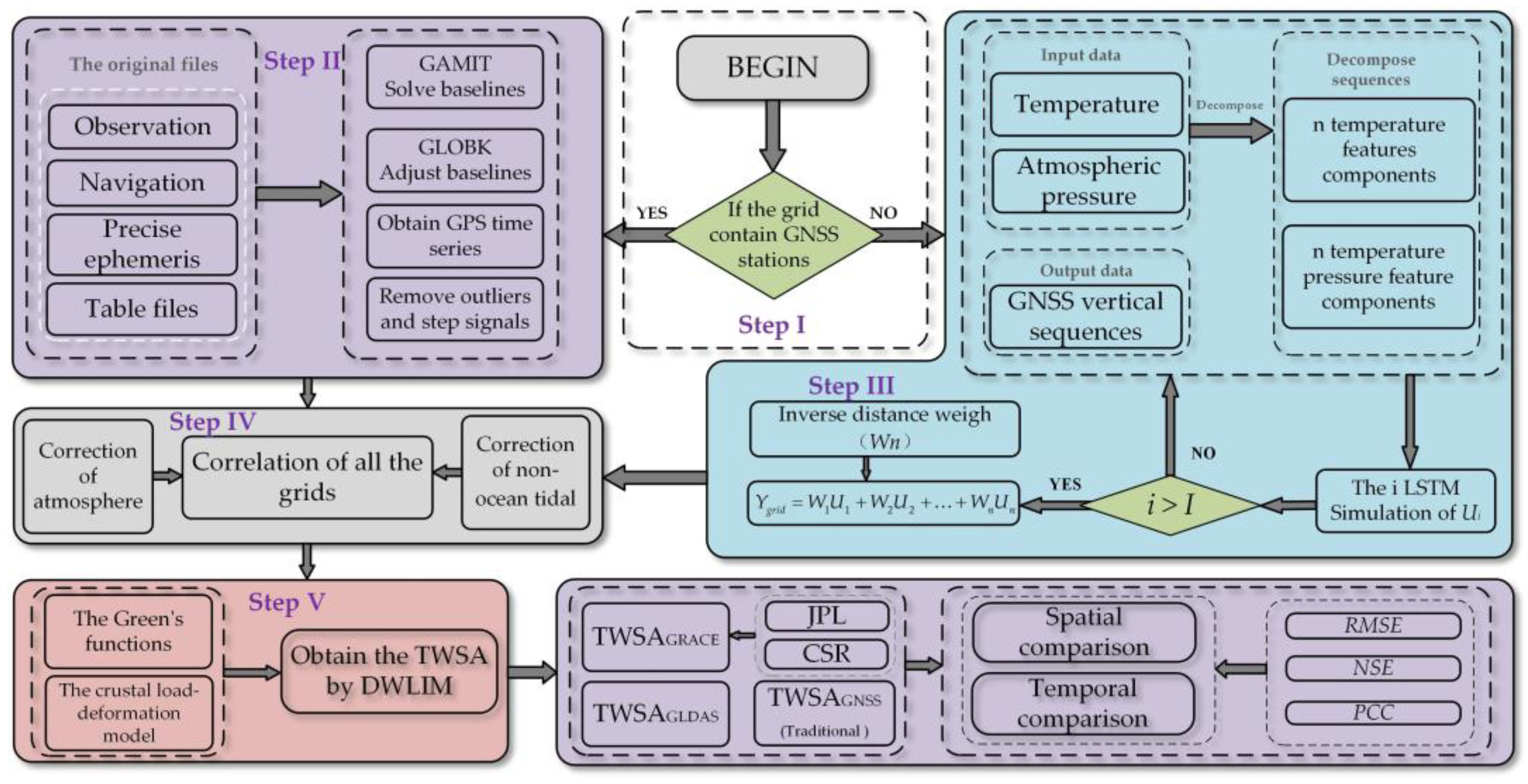
Broadly speaking, the hydrology and atmosphere on the surface exert stress on the continental crust. At the same time, the crust will produce corresponding elastic deformation when the stress is less than the elasticity of the crustal rocks [50,51]. Fortunately, GNSS can accurately observe crustal deformation with submillimeter accuracy [52]. In recent years, the crustal load-deformation model has been employed to invert the local TWSA in regions where GNSS stations are densely distributed [53,54,55]. However, the distribution of GNSS stations is uneven worldwide due to the influence of geographic conditions [12]. Sparsely distributed GNSS arrays cannot be used to accurately invert TWSA because of the limitation of the disk expansion radius. Therefore, it is one of the keys for accurately deriving TWSA to accurately simulate surface load-deformation in the unobserved regions. In this study, DWLIM was constructed by combining LSTM, the inverse distance weighting method, and the crustal load model. The specific process of DWLIM can be divided into the following five steps.
(1)
Step I: The study region is divided into 1° × 1° grids, and the grids are divided into two situations; specifically, the grids contain or do not contain GNSS stations. This algorithm will proceed to step II if the grid has GNSS stations. Moreover, the grid will be defined as an unobserved grid if it does not contain GNSS stations, and the vertical deformation will be simulated in step III.
(2)
Step II: The GNSS coordinate solution will be calculated by using observation, precision ephemeris, navigation, and table files based on GAMIT software [42]. The daily coordinates are calculated by the GLOBK software based on baseline data files (h-files), and series outliers and step terms that are three times larger than the standard deviation are removed.
(3)
Step III: The surface temperature sequence (ST) and atmosphere pressure sequence (SAP) are normalized on the grid scale. Furthermore, the normalized results are decomposed using the modified ensemble empirical mode decomposition (MEEMD) method to obtain 2 n feature sequences, including n ST and n SAP feature sequences. In the unobserved grid, the GNSS vertical deformation sequences are employed as the target sequences, and the 2 n feature sequences are utilized as the input sequences. Then, the LSTM regression method and the inverse distance weight method are employed to simulate the vertical displacement.
(4)
Step IV: The corrected sequences of atmospheric (NTAL) and non-tidal ocean loading (NTOL) are employed to obtain the hydrologic deformation in all the grids, including the GNSS grids and unobserved grids [56].
(5)
Step V: The TWSA results are obtained by combining the Green function and the inversion of the crustal load model with all hydrologic deformation. The flow chart of this study is shown in Figure 2.

2.3. Evaluation Index

In this study, the root mean square error (RMSE), Nash–Sutcliffe efficiency (NSE), and Pearson’s correlation coefficient (PCC) were utilized to evaluate the accuracy of DWLIM results [57,58,59], as follows.
R M S E = 1 n i = 1 n ( Y i X i ) 2
N S E = 1 i = 1 n ( Y i X i ) 2 i = 1 n ( X i X ¯ ) 2
P C C = i = 1 n ( X i X ¯ ) ( Y i Y ¯ ) i = 1 n ( X i X ¯ ) 2 i = 1 n ( Y i Y ¯ ) 2
where Y and X denote accurate and simulated data, respectively, and Y ¯ and X ¯ represent the mean value of data. The RMSE can be employed to evaluate the deviation of the inversion results from the actual values. The smaller the value of RMSE, the better the simulation accuracy. The NSE is mainly used to evaluate the performance of the hydrological model, and its value is not larger than 1. The larger the value, the better the hydrological model. When NSE is close to 0, it indicates that the effect of the hydrological model agrees with the average of observed values. The PCC is mainly employed to describe the linear correlation between two sequences. The PCC value is between −1 and 1. If the PCC value is closer to 1, the inversion result is more reliable.

3. Results

3.1. Inversion of TWSA Using DWLIM

3.1.1. Validation of Simulated Crustal Deformation

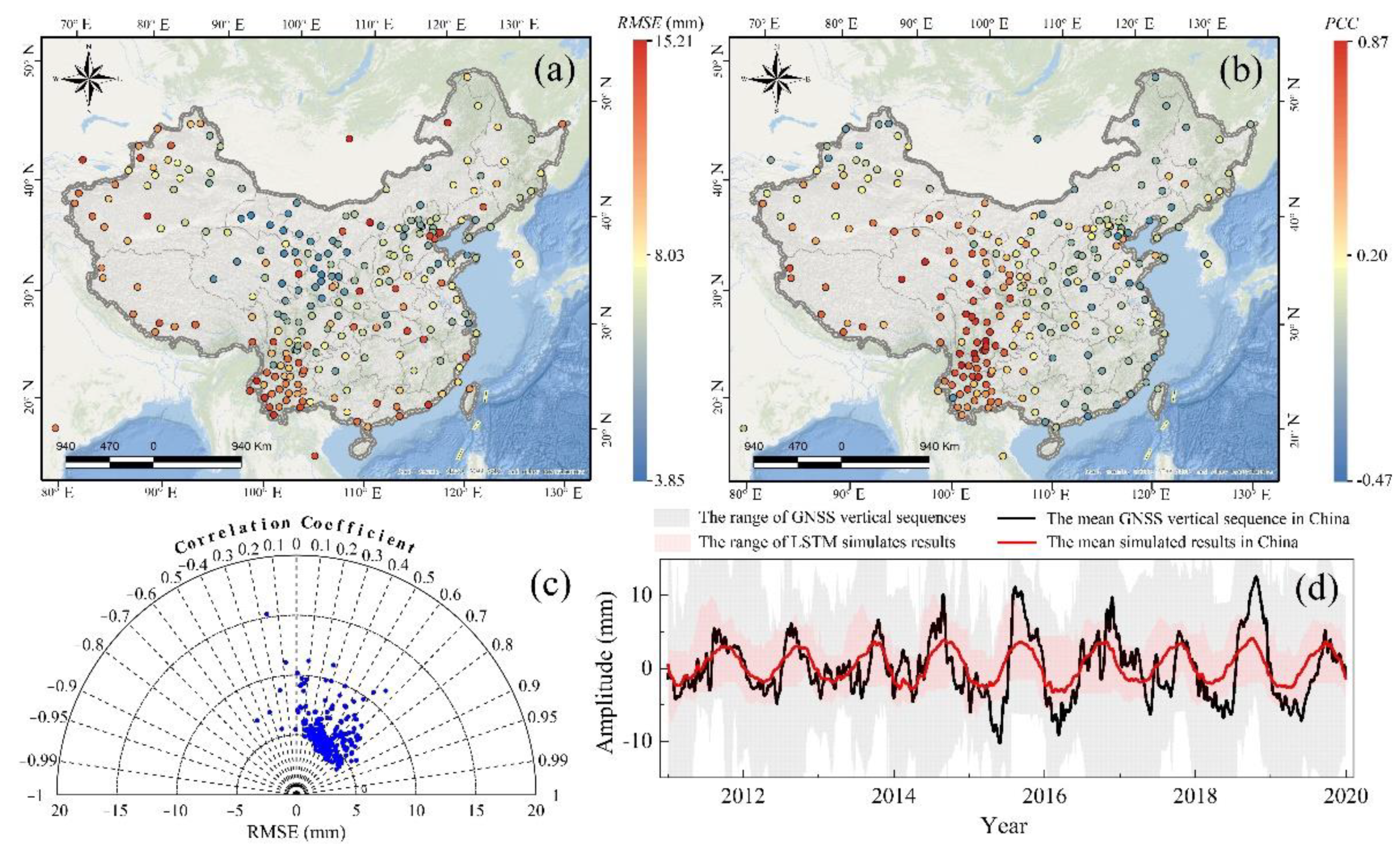
Seventy-five GNSS sites were selected in grids where the PCC values between the atmospheric pressure or temperature sequence and the GNSS sequence were greater than 0.5. The 75 GNSS sites were used as control sequences for the regression of LSTM, and 263 GNSS vertical sequences were employed for the validation of regression. It was regressed 74 times when the grid contained control GNSS stations, and it was regressed 75 times when the grid did not contain control GNSS stations. The inverse distance weight was employed to assign weights for 74 or 75 simulations. Furthermore, the GNSS vertical sequences were utilized as the true data to verify the accuracy of regression. The simulated results were contrasted with the GNSS vertical sequence according to the RMSE and PCC. The evaluation results are shown in Figure 3.
It can be seen from Figure 3 that most of the station sequences have RMSE values within 5 mm. The variability of the observation quality among GNSS sequences may lead to large RMSE values for some stations. The statistics of the evaluation index indicate that 68.63% of the RMSE values are within 6 mm. The PCC index was used to evaluate the consistency between the simulated sequences and the in situ measurements; the largest PCC value reaches 0.87, and its mean value is 0.53. Figure 3d shows the mean sequences of simulated results and the true data in China. The features of the annual amplitude are included in the simulated outcomes, and the mean simulated sequence is smoother than the GNSS vertical sequence.

3.1.2. Simulation of Hydrological Load-Deformation

(1)
Simulation of crustal deformation
In this study, the surface temperature and atmospheric pressure were utilized as the input data for the LSTM algorithm, and the models were established by using the 75 control GNSS vertical sequences. Furthermore, the MEEMD method was employed to decompose the surface temperature and atmospheric pressure sequences into 10 model components, IMF1–IMF10, respectively. The decomposition of the input sequences is shown in Figure 4, and the G456 grid is shown as an example.
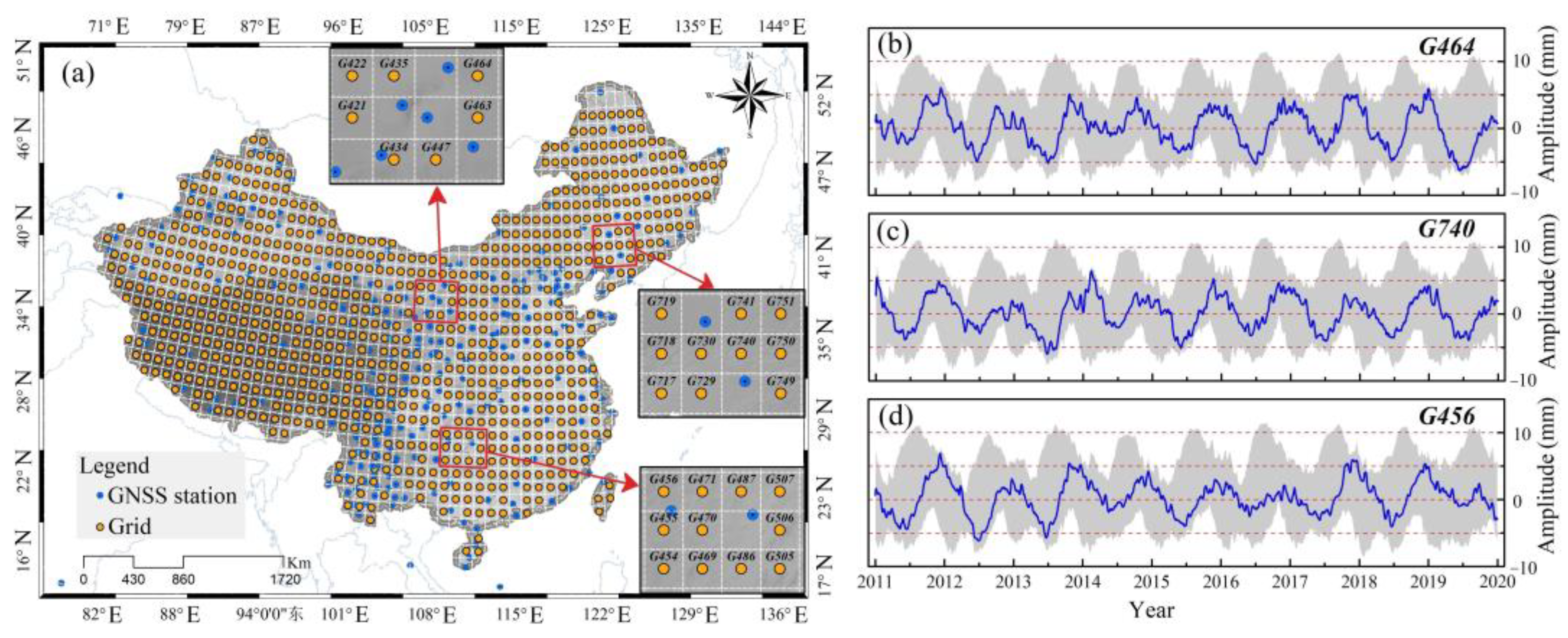
The IMF1 components in Figure 4a,b are the normalized original surface temperature and atmospheric pressure sequences, respectively. IMF2–IMF10 are the decomposed feature sequences from high to low frequencies. Specifically, the decomposed results reflect the trend and seasonal and residual terms of the series. In the LSTM regression method, the 10 IMF components were used as the input sequences, and the GNSS vertical deformation sequence was used as output data. Furthermore, the inverse distance weight was used to assign weights to the 75 simulated vertical displacements. The vertical simulated deformation was obtained in the unobserved grids. The distribution between the unknown grids and GNSS stations is shown in Figure 5a, and the simulated results of the unknown grid are shown in Figure 5b–d. The G464, G740, and G456 grids are shown as examples.
It can be seen from Figure 5a that the GNSS stations (blue points) are unevenly distributed, which cannot achieve the overall coverage of the crust over mainland China. Hence, the simulation of vertical deformation in unknown grids (yellow points) is essential. Figure 5b–d presents the simulated outcomes of vertical crustal deformation in unobserved grids using 20 IMF feature components for LSTM regression [60]. The results show that the period term and annual amplitude of the vertical crustal deformation can be well simulated according to this strategy, which provides a reasonable data basis for the inversion of TWSA.
(2)
Correction of all deformation sequences
This study used the NTAL and NTOL models as correction data to extract the crustal deformation caused by hydrological loading. The two corrected sequences were added to the crustal load-deformation time series in mainland China, including the GNSS vertical deformation and simulated results in the unobserved grids. Furthermore, the annual amplitudes of NATL and NOTL were calculated from 2011 to 2020, as shown in Figure 6a,b, respectively. To evaluate the performance of the correction as a whole, the mean sequence of the vertical deformation and hydrologic displacement was obtained, as shown in Figure 6c.
Figure 6 indicates that the mean values of the amplitude of the load-deformation of NATL and NOTL are equal to 3.62 and 0.22 mm, respectively. The raised region of the NTAL annual amplitude is mainly located in northern and eastern China, with a maximum of 5.5 mm. However, the maximum annual amplitude of NTOL is only 1.5 mm, and it is mainly distributed in the eastern coastal regions of China. It can be seen from Figure 6c that there are smaller variations in the amplitude and phase of the corrected sequence. The corrections of NTAL and NTOL provide accurate hydrological load-deformation sequences for DWLIM inversion of TWSA.

3.1.3. Inversion of TWSA Based on DWLIM

The Green function matrix of the point loadings was calculated, and the spatial resolution of the inversion outcomes is 0.25° × 0.25°. The expansion boundary range and β equal 2° and 0.01, respectively. Hydrologic displacement sequences were used as the input data for Equations (9) and (10) to calculate the daily TWSA in mainland China. To verify the accuracy of the DWLIM results, first-order term correction was applied to the inversion results in this study, including TWSA results of DWLIM, GRACE, and GLDAS. The calculated annual amplitudes and mean sequence of the TWSA results are shown in Figure 7a,b.
It can be seen from Figure 7 that the annual characteristics and amplitudes of TWSA sequences based on DWLIM can be effectively inverted. The raised regions of the annual amplitudes can be calculated using DWLIM, which are located in Yunnan Province, southern Tibet region, and southern North China Plain. Furthermore, this result is consistent with the inversion conclusions of previous studies [8]. To verify the accuracy of DWLIM, the outcomes of this study were compared with the inverted TWSA from the GRACE, GLDAS, and the traditional GNSS-derived method.

3.2. Validation of DWLIM

3.2.1. Spatial Verification of TWSA Results

In order to compare the accuracy of TWSA based on DWLIM, this study obtained TWSA using the traditional GNSS TWSA inversion method (TRAGNSS), GRACE-M datasets, and the GLDAS hydrological model. The detailed information of these outcomes is summarized in Table 2. Additionally, the annual amplitudes of these TWSA results were calculated, and the results are shown in Figure 8.
Figure 8 indicates that the DWLIM strategy can effectively invert the raised regions of annual amplitude in mainland China, such as southwestern Yunnan Province, southeast China, and the Qinghai–Tibet region. Overall, the spatial amplitude results of DWLIM are consistent with the outcomes of GRACE and GLDAS. However, the annual amplitude of DWLIM is slightly larger than that of GRACE and GLDAS. The reason is that the influence of crustal deformation is complex, and hydrological displacement cannot be completely extracted using NTAL and NTOL. Specifically, the raised regions of annual amplitude also contain northern Xinjiang and northern Heilongjiang. The spatial distribution of the annual amplitude based on the traditional GNSS-derived TWSA method contains speckle characteristics because of the distance limitation of the radius. Hence, the TWSA results based on the traditional GNSS inversion method can only infer the range around the GNSS stations. This will lead to missed signals in regions with sparse GNSS stations when smoothing, and it greatly limits the application of GNSS for TWSA inversion. Overall, the limitation of the disk radius on the GNSS TWSA inversion can be mitigated by simulating crustal deformation in the unknown grids.

3.2.2. Temporal Verification of the TWSA Results

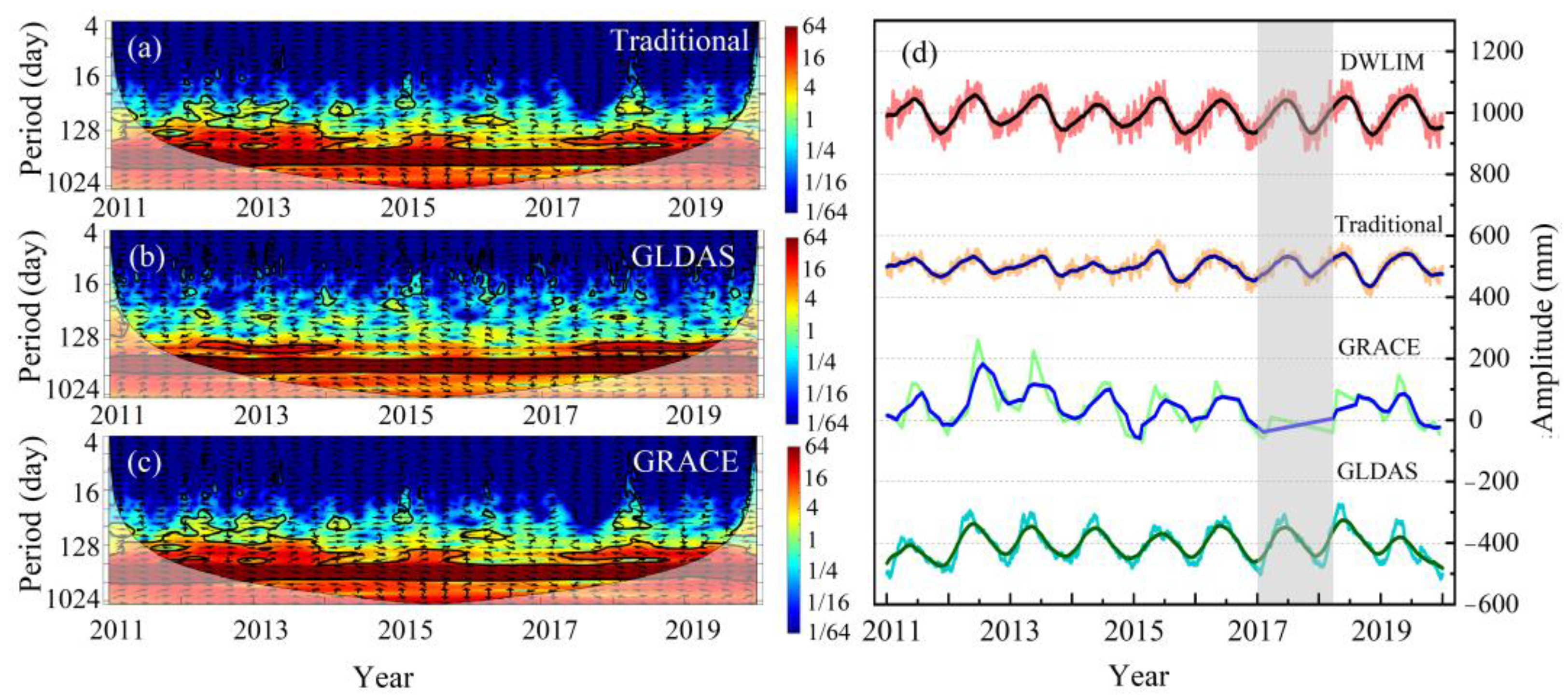
In order to verify the time series reliability of DWLIM, the DWLIM results were compared with the results of the traditional GNSS TWSA inversion method, GRACE, and GLDAS. To further analyze the relationship between DWLIM inversion results and the results of the other data, cross-wavelet analysis was performed, as shown in Figure 9a–c, respectively. In addition, the mean sequences of DWLIM, traditional GNSS, GRACE, and GLDAS over mainland China are shown in Figure 9d.
It can be seen from Figure 9a–c that the TWSA results of DWLIM are consistent with the TWSA of the traditional GNSS inversion method, GLDAS, and GRACE. In addition, the resonance periods between the DWLIM and the other data are about one year, which is shown by the red strip. DWLIM can effectively derive the annual and semiannual amplitudes of the TWSA sequences, which is consistent with the GRACE and GLDAS results (Figure 9d). However, the annual amplitude of DWLIM is slightly larger than the other TWSA results due to the difference in the observation strategy. Moreover, the corrected crustal deformation sequences also contain other deformation signals, resulting in the inability to separate single hydrological load-deformation sequences. The seasonal feature of the DWLIM results is more pronounced that of the traditional GNSS-derived results. To quantify the advantages of DWLIM over the traditional GNSS TWSA inversion method, this study evaluated the inversion results using PCC, NSE, and RMSE. The results are shown in Figure 10.
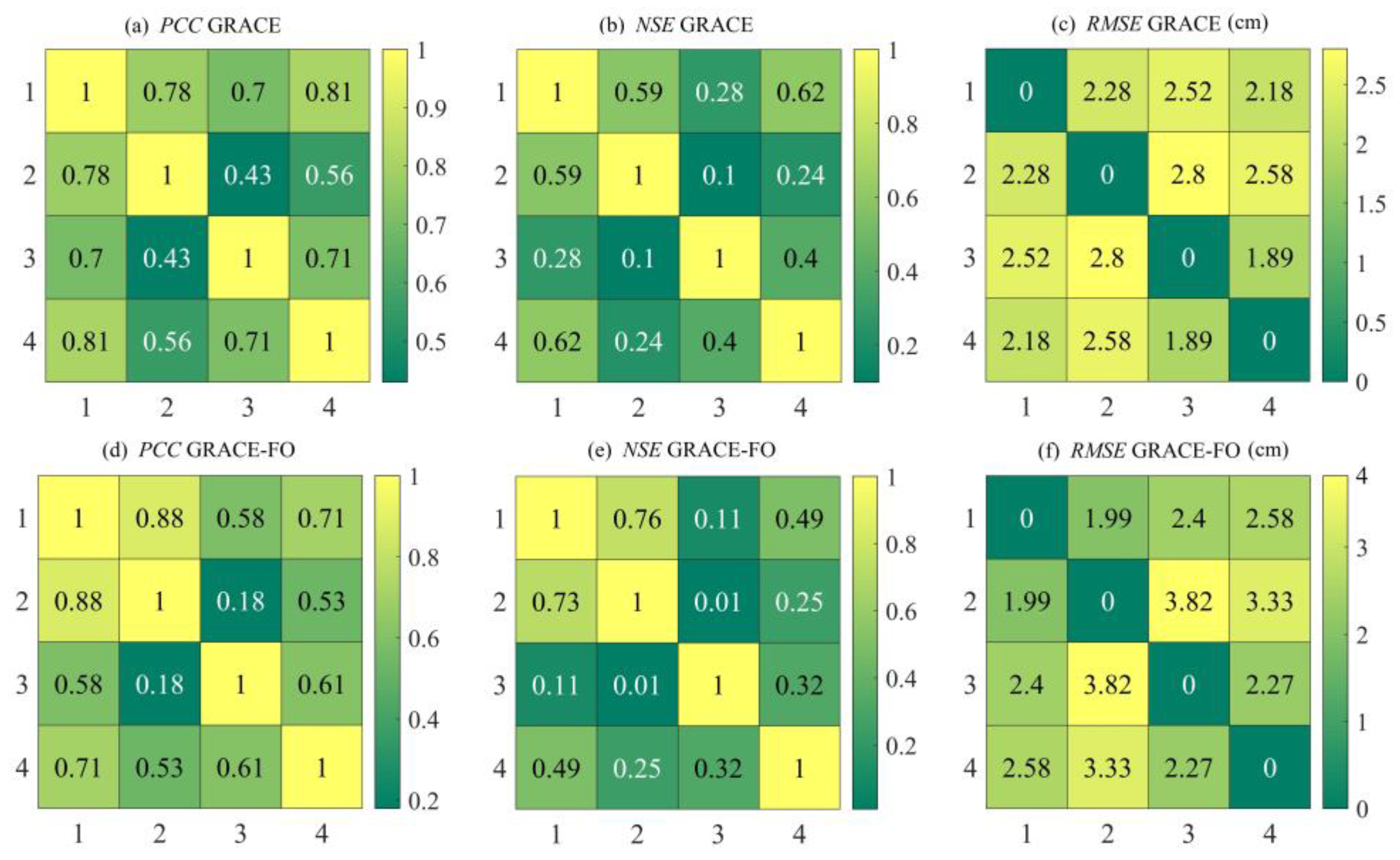
It can be seen from Figure 10 that, based on the evaluation indexes PCC, NSE, and RMSE, the TWSA results based on DWLIM are superior to the traditional GNSS-derived results. For the period of the GRACE mission (2011–2017), the maximum PCC, NSE, and RMSE indicators of DWLIM inversion results reach 0.81, 0.62, and 2.18 cm, respectively. For the period of the GRACE-FO mission (2018–2020), the maximum PCC, NSE, and RMSE of DWLIM inversion results reach 0.71, 0.49, and 2.4 cm. The results show that the TWSA results of DWLIM are more consistent with the GLDAS results, which is attributed to the monthly scale resolution of GRACE, leading to signal loss. Further statistics from the data show that the DWLIM results improve the PCC, NSE, and RMSE by 67.11, 128.15, and 22.75% on average compared to the traditional GNSS inversion method, respectively. The results further demonstrate that DWLIM can effectively derive TWSA in regions with sparse GNSS stations. Furthermore, the TWSA of DWLIM is better than the traditional GNSS-derived method in terms of spatial and temporal characteristics.

4. Discussion

4.1. Comparison with Precipitation over 10 River Basins

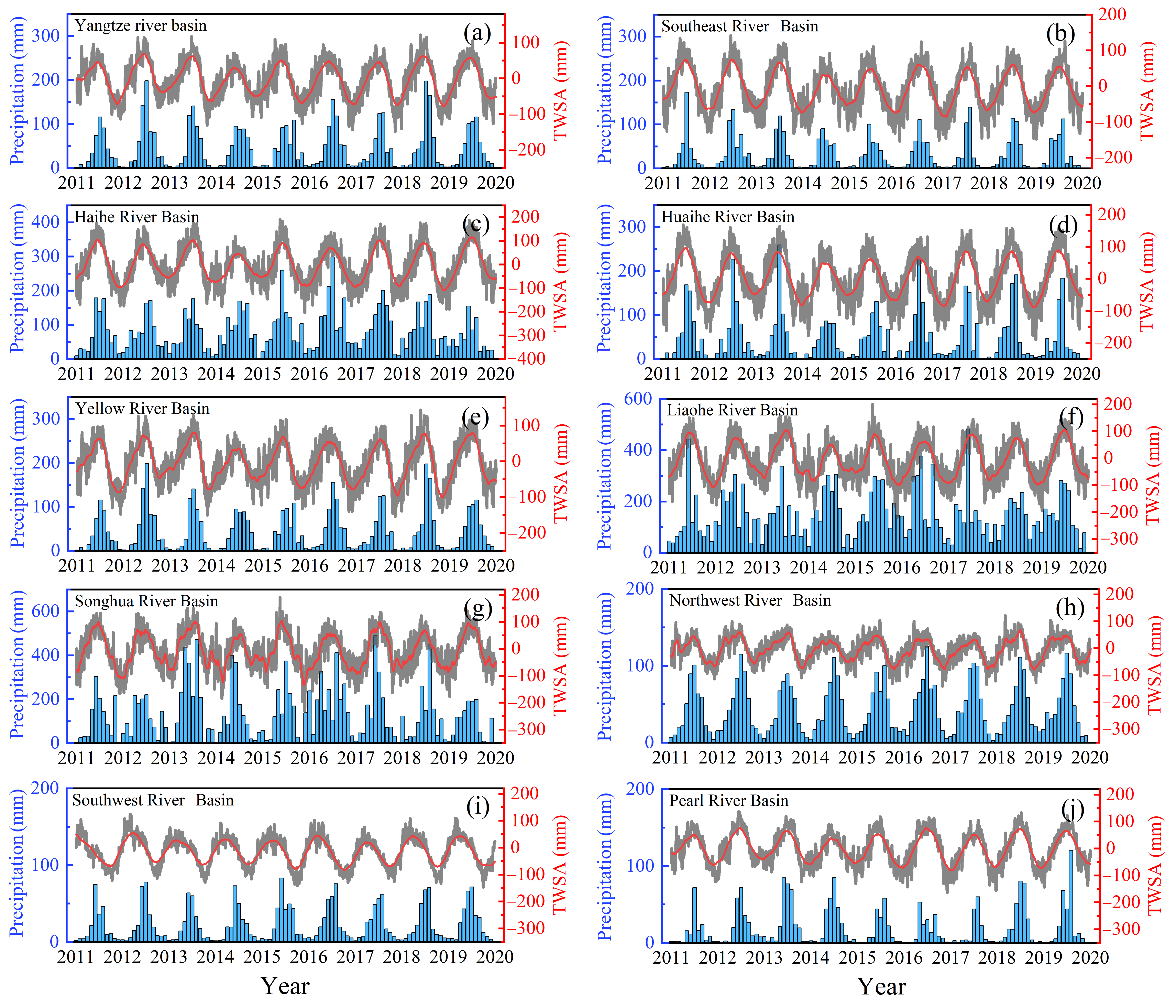
It is verified that DWLIM can effectively derive the TWSA in mainland China, and it can detect the raised regions of the TWSA annual amplitude. The crust shows a decreasing trend when the terrestrial water storage load increases. On the contrary, the crust shows an upward rebound trend when the terrestrial water storage load decreases. This study combined monthly precipitation products provided by the China Meteorological Administration (CMA) to analyze the variation characteristics of regional TWSA in mainland China. Furthermore, this study extracted the precipitation and TWSA of 10 river basins in China based on boundary files. TWSA was calculated by DWLIM, and the comparison is shown in Figure 11.
Figure 11 indicates that the annual amplitude of TWSA is generally positively correlated with the annual amplitude of precipitation. The mean precipitation sequences in the Songhua and Liaohe River basins are significantly higher than the others. Correspondingly, the amplitudes of TWSA results are also significantly higher than those in the other basins. The phase relationship between TWSA and precipitation in mainland China shows good consistency. This further indicates the reliability of TWSA in phase for DWLIM inversion in mainland China. However, the sequences of TWSA based on DWLIM and precipitation contain delays on the scale of months due to the time needed for the elastic deformation of TWSA. The results of TWSA and precipitation are consistent with previous studies [8]. The seasonal items of TWSA outcomes are more regular than previous TWSA results. Furthermore, the amplitude performance of TWSA and precipitation can also be used to evaluate the arid situation over the river basins. At the same time, it can also be seen that there is high-frequency noise in the time series of TWSA sequences, which also affects the inversion or prediction of TWSA. It is mainly caused by systematic noise from ionospheric, tropospheric, clock error, and multipath effects during GNSS observations [52,61]. Therefore, we will also focus on the noise classification and removal of GNSS vertical sequences to provide cleaner sequences for TWSA inversion in future research.

4.2. Discussion of the Difference between Products

In this study, we utilized DWLIM, GRACE, GLDAS, and the traditional GNSS method to calculate TWSA over mainland China. We compared these TWSA outcomes from the perspectives of spatial amplitude (Figure 8) and time series (Figure 9). It can be seen from Figure 8 that DWLIM is consistent with GRACE and GLDAS over most regions. However, there are also some differences between DWLIM and other products over certain regions, such as Beijing. The reasons for this can be summarized as follows. First, there are only two available GNSS stations (BJFS and BJSH) over Beijing. Second, vertical crustal deformation in the entirety of the North China Plain is complex and has been greatly influenced by human activity, which can cause inaccuracies in the simulated deformation. Third, the GNSS inversion result is also a little higher than the other products because the load-deformation contains other components. Therefore, there may be some differences between the results of DWLIM and GRACE and GLDAS in some regions. Furthermore, it can be seen from Figure 8a,b that DWLIM can effectively suppress the speckle effect caused by uneven distribution of GNSS stations. In future research, we will focus on extracting cleaner crustal hydrological load-deformation to increase the accuracy of the inversion results.

5. Conclusions

The main research results can be summarized in the following three points.
(1)
To increase the derived accuracy for TWSA, DWLIM was constructed by combining LSTM, inverse distance weight, and the crustal load-deformation model. First, the study region was divided into 1° × 1° grids, and then we determined whether the grid contained GNSS stations. Second, this study selected the surface temperature and atmospheric pressure as input data, and the GNSS vertical sequences were utilized as the output data. Each unobserved grid was simulated 263 times, and the inverse distance weight was used to calculate the weighted sequence. Third, the NTAL and NTOL models were employed to correct vertical deformation over all of the grids to obtain the hydrologic distribution. Finally, all of the corrected sequences were used as the input data for the crustal load model to derive TWSA in mainland China.
(2)
To verify the accuracy of DWLIM, the TWSA results of DWLIM were compared with the traditional GNSS TWSA inversion, GRACE, and GLDAS results. The results indicate that the annual amplitude distribution of DWLIM is smoother than the traditional GNSS inversion results. The strategy of DWLIM greatly suppresses the effect of a small disk expansion radius. The maximum PCC, NSE, and RMSE of DWLIM results compared with GRACE and GLDAS are equal to 0.81, 0.62, and 2.18 cm, respectively, which are improved by 67.11, 128.15, and 22.75% compared with the traditional GNSS-derived TWSA method, respectively. Overall, the DWLIM can effectively invert the TWSA in regions with an uneven distribution of GNSS stations.
(3)
This study employed precipitation data to analyze the relationship between TWSA and rainfall. We inverted TWSA based on DWLIM in 10 river basins of mainland China. The results indicate that TWSA is positively correlated with precipitation. The annual amplitudes of precipitation and TWSA in the Songhua River basin and the Liaohe River basin are significantly higher than those in other basins. Furthermore, the wave peaks of precipitation are in good agreement with the peaks of TWSA, which are located in June or July. This result further verifies the reliability of the DWLIM inversion results in terms of phase.

Author Contributions

All authors collaborated to conduct this study; Y.S.: scientific analysis, manuscript writing, and editing. W.Z. and W.Y.: experimental design, project management, and review and editing. A.X. and H.Z.: review and editing. Q.W. and Z.C.: editing. All authors contributed to the article and approved the submitted version. Y.S., W.Z. and W.Y. contributed equally to this paper. All authors have read and agreed to the published version of the manuscript.

Funding

This work was supported by the National Natural Science Foundation of China (under grants 41774014 and 41574014), the Liaoning Revitalization Talents Program (under grants XLYC2002082, XLYC2002101, and XLYC2008034), the Frontier Science and Technology Innovation Project and the Innovation Workstation Project of Science and Technology Commission of the Central Military Commission (under grant 085015), and the Outstanding Youth Fund of China Academy of Space Technology.

Institutional Review Board Statement

Not applicable.

Informed Consent Statement

Not applicable.

Data Availability Statement

Not applicable.

Acknowledgments

The authors greatly appreciate the China Earthquake Administration for the GNSS data of Crustal Movement Observation Network of China (CMONOC: http://www.cgps.ac.cn, accessed on 9 December 2021) and the CSR (http://www.csr.utexas.edu/grace/, accessed on 6 August 2021) and JPL (https://grace.jpl.nasa.gov/, accessed on 9 December 2021), which provided the GRACE Mascon data. The authors would like to thank NASA for providing the dataset of GLDAS (http://agdisc.gsfc.nasa.gov/dods/, accessed on 9 December 2021). We thank ECMWF for providing the reanalysis data of the atmospheric pressure (https://www.ecmwf.int/, accessed on 21 December 2021). We thank the Earth system modeling group at Deutsches GeoForschungsZentrum for providing the corrected model (ESMGFZ: http://esmdata.gfz-potsdam.de:8080/repository/, accessed on 21 December 2021). We also thank China Meteorological Administration (CMA: http://data.cma.cn/, accessed on 21 December 2021) for providing the precipitation data.

Conflicts of Interest

The authors declare no conflict of interest.

References

  1. Long, D.; Shen, Y.; Sun, A.; Hong, Y.; Longuevergne, L.; Yang, Y.; Li, B.; Chen, L. Drought and flood monitoring for a large karst plateau in southwest China using extended GRACE data. Remote Sens. Environ. 2014, 155, 145–160. [Google Scholar] [CrossRef]
  2. Ahi, G.O.; Cekim, H.O. Long-term temporal prediction of terrestrial water storage changes over global basins using GRACE and limited GRACE-FO data. Acta Geod. Geophys. 2021, 56, 321–344. [Google Scholar] [CrossRef]
  3. Shen, Y.; Zheng, W.; Yin, W.; Xu, A.; Zhu, H.; Yang, S.; Su, K. Inverted algorithm of terrestrial water-storage anomalies based on machine learning combined with load model and its application in southwest China. Remote Sens. 2021, 13, 3358. [Google Scholar] [CrossRef]
  4. Yin, W.; Hu, L.; Han, S.C.; Zhang, M.; Teng, Y. Reconstructing terrestrial water storage variations from 1980 to 2015 in the Beishan area of China. Geofluids 2019, 2019, 3874742. [Google Scholar] [CrossRef]
  5. Li, W.; Wang, D.; Liu, S.; Zhu, Y.; Yan, Z. Reclamation of Cultivated Land Reserves in Northeast China: Indigenous Ecological Insecurity Underlying National Food Security. Int. J. Environ. Res. Public Health 2020, 17, 1211. [Google Scholar] [CrossRef] [Green Version]
  6. Davis, J.L.; Elosegui, P.; Mitrovica, J.X.; Tamisiea, M.E. Climate-driven deformation of the solid Earth from GRACE and GPS. Geophys. Res. Lett. 2004, 31, L24605. [Google Scholar] [CrossRef] [Green Version]
  7. Li, W.; Wang, W.; Zhang, C.; Wen, H.; Zhong, Y.; Zhu, Y.; Li, Z. Bridging terrestrial water storage anomaly during GRACE/GRACE-FO gap using SSA method: A case study in China. Sensors 2019, 19, 4144. [Google Scholar] [CrossRef] [Green Version]
  8. Jiang, Z.; Hsu, Y.-J.; Yuan, L.; Cheng, S.; Li, Q.; Li, M. Estimation of daily hydrological mass changes using continuous GNSS measurements in mainland China. J. Hydrol. 2021, 598, 126349. [Google Scholar] [CrossRef]
  9. Jin, S.; Zhang, T. Terrestrial water storage anomalies associated with drought in southwestern USA from GPS observations. Surv. Geophys. 2016, 37, 1139–1156. [Google Scholar] [CrossRef]
  10. Yin, W.; Hu, L.; Zhang, M.; Wang, J.; Han, S. Statistical downscaling of GRACE-derived groundwater storage using ET data in the North China Plain. J. Geophys. Res. Atmos. 2018, 123, 5973–5987. [Google Scholar] [CrossRef]
  11. Tangdamrongsub, N.; Šprlák, M. The assessment of hydrologic- and flood-induced land deformation in data-sparse regions using GRACE/GRACE-FO data assimilation. Remote Sens. 2021, 13, 235. [Google Scholar] [CrossRef]
  12. Jiang, Z.; Hsu, Y.-J.; Yuan, L.; Huang, D. Monitoring time-varying terrestrial water storage changes using daily GNSS measurements in Yunnan, southwest China. Remote Sens. Environ. 2021, 254, 112249. [Google Scholar] [CrossRef]
  13. Schmidt, R.; Flechtner, F.; Meyer, U.; Neumayer, K.-H.; Dahle, C.; Knig, R.; Kusche, J. Hydrological signals observed by the GRACE satellites. Surv. Geophys. 2008, 29, 319–334. [Google Scholar] [CrossRef]
  14. Xiang, Y.; Yue, J.; Cong, K.; Xing, Y.; Cai, D. Characterizing the seasonal hydrological loading over the asian continent using GPS, GRACE, and hydrological model. Pure Appl. Geophys. 2019, 176, 5051–5068. [Google Scholar] [CrossRef]
  15. Syed, T.H.; Famiglietti, J.S.; Rodell, M.; Chen, J.; Wilson, C.R. Analysis of terrestrial water storage changes from GRACE and GLDAS. Water Resour. Res. 2008, 44, 2433–2448. [Google Scholar] [CrossRef]
  16. Moghim, S. Assessment of water storage changes using GRACE and GLDAS. Water Resour. Manag. 2020, 34, 685–697. [Google Scholar] [CrossRef]
  17. Zheng, W.; Xu, Z.; Zhong, M.; Yun, M. Efficient accuracy improvement of GRACE global gravitational field recovery using a new inter-satellite range interpolation method. J. Geodyn. 2012, 53, 1–7. [Google Scholar] [CrossRef]
  18. Feng, W.; Zhong, M.; Lemoine, J.M.; Biancale, R.; Hsu, H.T.; Xia, J. Evaluation of groundwater depletion in North China using the Gravity Recovery and Climate Experiment (GRACE) data and ground-based measurements. Water Resour. Res. 2013, 49, 2110–2118. [Google Scholar] [CrossRef]
  19. Fok, H.S.; Liu, Y. An improved GPS-inferred seasonal terrestrial water storage using terrain-corrected vertical crustal displacements constrained by GRACE. Remote Sens. 2019, 11, 1433. [Google Scholar] [CrossRef] [Green Version]
  20. Fu, Y.; Argus, D.F.; Freymueller, J.T.; Heflin, M.B. Horizontal motion in elastic response to seasonal loading of rain water in the Amazon Basin and monsoon water in Southeast Asia observed by GPS and inferred from GRACE. Geophys. Res. Lett. 2013, 40, 6048–6053. [Google Scholar] [CrossRef]
  21. Velicogna, I. Increasing rates of ice mass loss from the Greenland and Antarctic ice sheets revealed by GRACE. Geophys. Res. Lett. 2009, 36, L19503. [Google Scholar] [CrossRef] [Green Version]
  22. Liu, R.; Zou, R.; Li, J.; Zhang, C.; Zhao, B.; Zhang, Y. Vertical displacements driven by groundwater storage changes in the North China Plain detected by GPS observations. Remote Sens. 2018, 10, 259–272. [Google Scholar] [CrossRef] [Green Version]
  23. Zhong, B.; Li, X.; Chen, J.; Li, Q.; Liu, T. Surface mass variations from GPS and GRACE/GFO: A case study in southwest China. Remote Sens. 2020, 12, 1835–1846. [Google Scholar] [CrossRef]
  24. Pan, Y.; Zhang, C.; Gong, H.L.; Yeh, P.J.F.; Shen, Y.; Guo, Y.; Huang, Z.; Li, X. Detection of human-induced evapotranspiration using GRACE satellite observations in the Haihe River Basin of China. In Proceedings of the Egu General Assembly Conference, Vienna, Austria, 23–28 April 2017; pp. 190–199. [Google Scholar]
  25. Vishwakarma, B.D.; Zhang, J.; Sneeuw, N. Downscaling GRACE total water storage change using partial least squares regression. Sci. Data 2021, 8, 95. [Google Scholar] [CrossRef] [PubMed]
  26. Hussain, D.; Khan, A.A.; Hassan, S.N.U.; Naqvi, S.A.A.; Jamil, A. A time series assessment of terrestrial water storage and its relationship with hydro-meteorological factors in Gilgit-Baltistan region using GRACE observation and GLDAS-Noah model. SN Appl. Sci. 2021, 3, 533. [Google Scholar] [CrossRef]
  27. Chen, C.; Zou, R.; Liu, R.L. Vertical deformation of seasonal hydrological loading in southern tibet detected by joint analysis of GPS and GRACE. Geomat. Inf. Sci. Wuhan Univ. 2018, 43, 669–675. [Google Scholar]
  28. Dagan, G. Solute transport in heterogeneous porous formations. Water Resour. Res. 2004, 55, 671–682. [Google Scholar] [CrossRef]
  29. Fu, Y.; Freymueller, J.T. Seasonal and long-term vertical deformation in the Nepal Himalaya constrained by GPS and GRACE measurements. J. Geophys. Res. Solid Earth 2012, 117, B03407. [Google Scholar] [CrossRef]
  30. Wahr, J.; Khan, S.A.; Dam, T.V.; Liu, L.; Angelen, J.V.; Van, D.; Meertens, C.M. The use of GPS horizontals for loading studies, with applications to northern California and southeast Greenland. J. Geophys. Res. Solid Earth 2013, 118, 1795–1806. [Google Scholar] [CrossRef] [Green Version]
  31. Gautam, P.K.; Gahalaut, V.K.; Prajapati, S.K.; Kumar, N.; Yadav, R.K.; Rana, N.; Dabral, C.P. Continuous GPS measurements of crustal deformation in Garhwal-Kumaun Himalaya. Quat. Int. 2017, 462, 124–129. [Google Scholar] [CrossRef]
  32. Argus, D.F.; Fu, Y.; Landerer, F.W. Seasonal variation in total water storage in California inferred from GPS observations of vertical land motion. Geophys. Res. Lett. 2014, 41, 1971–1980. [Google Scholar] [CrossRef]
  33. Argus, D. Sustained water changes in California during drought and heavy precipitation inferred from GPS, InSAR, and GRACE. In Proceedings of the Agu Fall Meeting, San Francisco, CA, USA, 14–18 December 2015. [Google Scholar]
  34. Borsa, A.A.; Agnew, D.C.; Cayan, D.R. Ongoing drought-induced uplift in the western United States. Science 2014, 345, 1587–1590. [Google Scholar] [CrossRef] [PubMed]
  35. Enzminger, T.L.; Small, E.E.; Borsa, A.A. Accuracy of snow water equivalent estimated from GPS vertical displacements: A synthetic loading case study for western U.S. mountains. Water Resour. Res. 2018, 54, 581–599. [Google Scholar] [CrossRef]
  36. Heki, K. Dense gps array as a new sensor of seasonal changes of surface loads. In The State of the Planet: Frontiers and Challenges in Geophysics; American Geophysical Union: Washington, DC, USA, 2004; Volume 150, pp. 177–196. [Google Scholar]
  37. Adusumilli, S.; Borsa, A.A.; Fish, M.A.; McMillan, H.K.; Silverii, F. A decade of water storage changes across the contiguous united states from GPS and satellite gravity. Geophys. Res. Lett. 2019, 46, 13006–13015. [Google Scholar] [CrossRef]
  38. Liu, R.; Li, J.; Fok, H.; Shum, C.K.; Li, Z. Earth surface deformation in the North China Plain detected by joint analysis of GRACE and GPS data. Sensors 2014, 14, 19861–19876. [Google Scholar] [CrossRef] [Green Version]
  39. Pan, Y.; Shen, W.B.; Ding, H.; Hwang, C.; Li, J.; Zhang, T. The quasi-biennial vertical oscillations at global GPS stations: Identification by ensemble empirical mode decomposition. Sensors 2015, 15, 26096–26114. [Google Scholar] [CrossRef]
  40. Zheng, G.; Wang, H.; Wright, T.J.; Lou, Y.D.; Zhang, R.; Zhang, W.X.; Shi, C.; Huang, J.F.; Wei, N. Crustal deformation in the India-Eurasia collision zone from 25 years of GPS measurements: Crustal deformation in Asia from GPS. J. Geophys. Res. Solid Earth 2017, 122, 9290–9312. [Google Scholar] [CrossRef]
  41. Shen, Y.; Zheng, W.; Yin, W.; Xu, A.; Zhu, H. Feature extraction algorithm using a correlation coefficient combined with the VMD and its application to the GPS and GRACE. IEEE Access 2021, 9, 17507–17519. [Google Scholar] [CrossRef]
  42. Herring, T.A.; King, R.W.; Mcclusky, S.C. GAMIT Reference Manual. 2010. [Google Scholar]
  43. Xue, K. Combined GRACE and GPS to Study Terrestrial Water Storage; Chang’an University: Xi’an, China, 2017. [Google Scholar]
  44. Ji, L.; Senay, G.B.; Verdin, J.P. Evaluation of the global land data assimilation system (GLDAS) air temperature data products. J. Hydrometeorol. 2015, 16, 150731131106004. [Google Scholar] [CrossRef]
  45. Yu, X.; Zhang, L.; Zhou, T.; Liu, J. The Asian subtropical westerly jet stream in CRA-40, ERA5, and CFSR reanalysis data: Comparative assessment. J. Meteorol. Res. 2021, 35, 46–63. [Google Scholar] [CrossRef]
  46. Hochreiter, S.; Schmidhuber, J. Long Short-Term Memory. Neural Comput. 1997, 9, 1735–1780. [Google Scholar] [CrossRef] [PubMed]
  47. Yao, Y.; Sfarra, S.; Ibarra-Castanedo, C.; You, R.; Maldague, X.P.V. The multi-dimensional ensemble empirical mode decomposition (MEEMD). J. Therm. Anal. Calorim. 2017, 128, 1841–1858. [Google Scholar] [CrossRef]
  48. Wang, H.; Xiang, L.; Jia, L.; Jiang, L.; Wang, Z.; Hu, B.; Gao, P. Load love numbers and Green’s functions for elastic earth models PREM, iasp91, ak135, and modified models with refined crustal structure from Crust 2.0. Comput. Geosci. 2012, 49, 190–199. [Google Scholar] [CrossRef]
  49. Wang, Z.; Ou, J. Determining the ridge parameter in a ridge estimation using L-curve method. Geomat. Inf. Sci. Wuhan Univ. 2004, 29, 235–238. [Google Scholar]
  50. Abdrakhmatov, K.Y.; Aldazhanov, S.A.; Hager, B.H.; Hamburger, M.W.; Herring, T.A.; Kalabaev, K.B.; Makarov, V.I.; Molnar, P.; Panasyuk, S.V.; Prilepin, M.T.; et al. Relatively recent construction of the Tien Shan inferred from GPS measurements of present-day crustal deformation rates. Nature 1996, 384, 450–453. [Google Scholar] [CrossRef]
  51. Dam, T.v.; Wahr, J.; Lavallée, D. A comparison of annual vertical crustal displacements from GPS and Gravity Recovery and Climate Experiment (GRACE) over Europe. J. Geophys. Res. Solid Earth 2007, 112, 404–415. [Google Scholar]
  52. Gülal, E.; Erdo An, H.; Tiryakio Lu, B. Research on the stability analysis of GNSS reference stations network by time series analysis. Digit. Signal. Process. 2013, 23, 1945–1957. [Google Scholar] [CrossRef]
  53. Ding, Y.H.; Huang, D.F.; Shi, Y.L.; Jiang, Z.S.; Chen, T. Determination of vertical surface displacements in Sichuan using GPS and GRACE measurements. Chin. J. Geophys. 2018, 061, 4777–4788. [Google Scholar]
  54. He, M.; Shen, W.; Pan, Y.; Chen, R.; Guo, G. Temporal–Spatial surface seasonal mass changes and vertical crustal deformation in south china block from GPS and GRACE measurements. Sensors 2017, 18, 99. [Google Scholar] [CrossRef] [Green Version]
  55. Fu, Y.; Argus, D.F.; Landerer, F.W. GPS as an independent measurement to estimate terrestrial water storage variations in Washington and Oregon. J. Geophys. Res. Solid Earth 2015, 120, 552–566. [Google Scholar] [CrossRef]
  56. Dill, R.; Dobslaw, H. Numerical simulations of global-scale high-resolution hydrological crustal deformations. J. Geophys. Res. Solid Earth 2013, 118, 5008–5017. [Google Scholar] [CrossRef]
  57. Chai, T.; Draxler, R.R. Root mean square error (RMSE) or mean absolute error (MAE) aguments against avoiding RMSE in the literature. Geosci. Model. Dev. 2014, 7, 1247–1250. [Google Scholar] [CrossRef] [Green Version]
  58. Heinzl, H.; Mittlböck, M. Pseudo R-squared measures for poisson regression models with over- or underdispersion. Comput. Stat. Data Anal. 2003, 44, 253–271. [Google Scholar] [CrossRef]
  59. Gupta, H.V.; Kling, H.; Yilmaz, K.K.; Martinez, G.F. Decomposition of the mean squared error and NSE performance criteria: Implications for improving hydrological modelling. J. Hydrol. 2009, 377, 80–91. [Google Scholar] [CrossRef] [Green Version]
  60. Zimmerman, D.; Pavlik, C.; Ruggles, A.; Armstrong, M.P. An Experimental Comparison of Ordinary and Universal Kriging and Inverse Distance Weighting. Math. Geol. 1999, 31, 375–390. [Google Scholar] [CrossRef]
  61. Klos, A.; Karegar, M.A.; Kusche, J.; Springer, A. Quantifying noise in daily GPS height time series: Harmonic function versus GRACE-assimilating modeling approaches. IEEE Geosci. Remote Sens. Lett. 2020, 18, 627–631. [Google Scholar] [CrossRef]
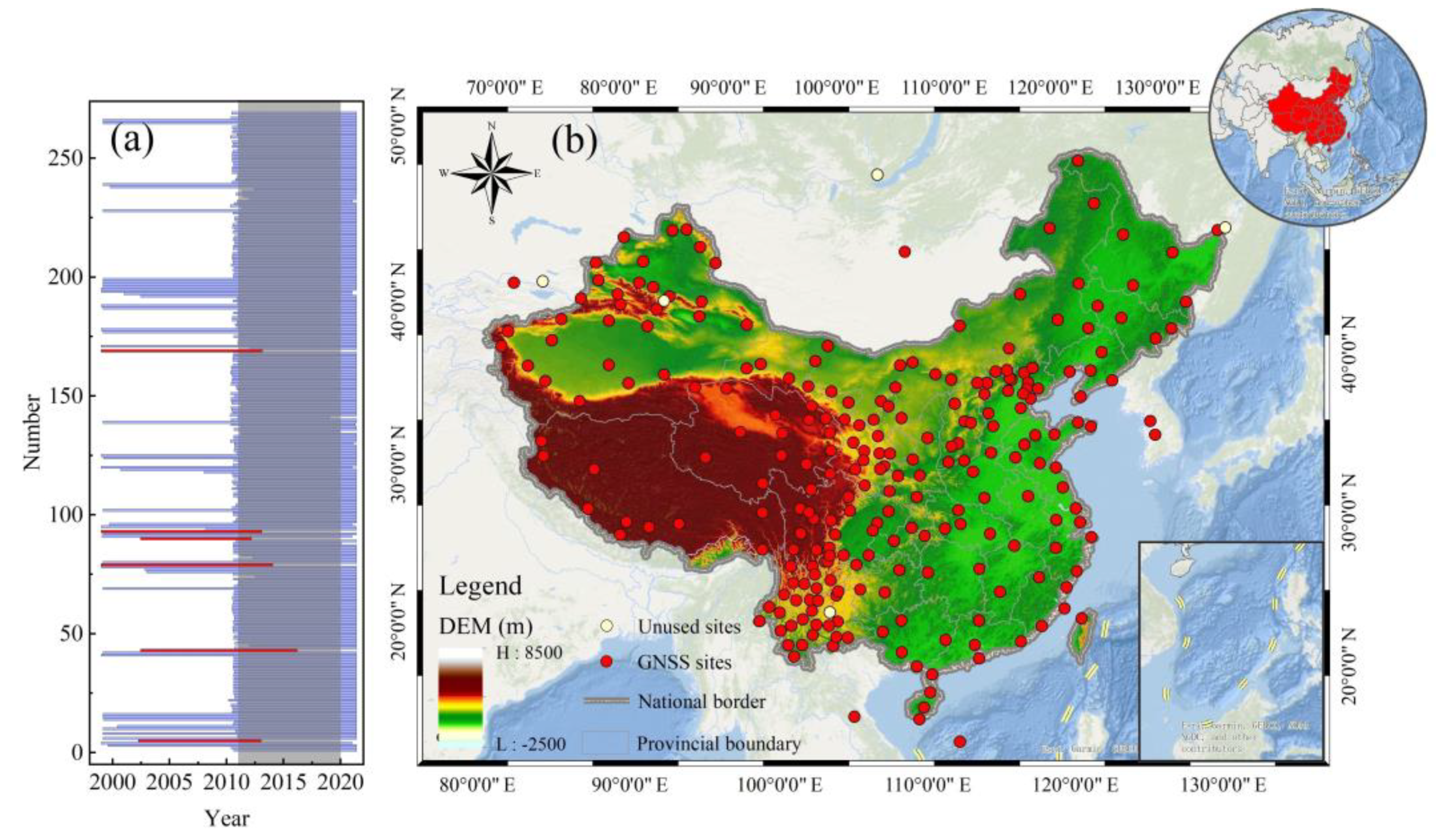
Figure 1. Distribution of continuous observation stations over mainland China. (a) The period of each GNSS station. (b) The distribution map of GNSS stations.
Remotesensing 14 00535 g001
Figure 2. The flow chart of DWLIM.
Remotesensing 14 00535 g002
Figure 3. The verification outcomes of simulated crustal deformation. (a) The RMSE between the simulation and in situ measurement; (b) the PCC between the derived sequence and true data; (c) the Taylor figure of the simulated results; (d) the mean simulated sequences in mainland China.
Remotesensing 14 00535 g003
Figure 4. The result of normalization and decomposition in the unobserved grids, showing G456 as an example. (a) The result of the temperature sequence; (b) the result of the atmospheric sequence.
Remotesensing 14 00535 g004
Figure 5. The simulated results in the unobserved grids. (a) The distribution of the unobserved grids and GNSS sites; (b) the result of G464; (c) the result of G740; (d) the result of G456.
Remotesensing 14 00535 g005
Figure 6. The corrected performance using NTAL and NTOL. (a) The annual amplitude distribution of atmospheric crustal deformation; (b) the annual amplitude distribution of non-ocean crustal deformation; (c) the mean sequences of the corrected results.
Remotesensing 14 00535 g006
Figure 7. The derived TWSA results based on DWLIM in China. (a) The distribution of TWSA annual amplitude in China; (b) the mean time series of TWSA in mainland China.
Remotesensing 14 00535 g007
Figure 8. The spatial distribution of TWSA annual amplitude in mainland China. (a) The result of DWLIM; (b) the result of traditional inversion method based on GNSS; (c) the result of GRACE; (d) the result of GLDAS.
Remotesensing 14 00535 g008
Figure 9. The analysis and time series of TWSA results. (a) Wavelet analysis between DWLIM and traditional GNSS TWSA inversion method; (b) wavelet analysis between DWLIM and GLDAS; (c) wavelet analysis between DWLIM and GRACE; (d) the mean time series of the TWSA results in mainland China.
Remotesensing 14 00535 g009
Figure 10. The heat figure of the evaluation index based on DWLIM. (a) The value of PCC in the GRACE period; (b) the value of NSE in the GRACE period; (c) the value of RMSE in the GRACE period; (d) the value of PCC in the GRACE-FO period; (e) the value of NSE in the GRACE-FO period; (f) the value of RMSE in the GRACE-FO period.
Remotesensing 14 00535 g010
Figure 11. The comparison of precipitation and TWSA over 10 basins in mainland China. (a) Yangtze River basin; (b) Southeast River basin; (c) Haihe River basin; (d) Huaihe River basin; (e) Yellow River basin; (f) Liaohe River basin; (g) Songhua River basin; (h) Northwest River basin; (i) Southwest River basin; (j) Pearl River basin.
Remotesensing 14 00535 g011
Table 1. Table of GNSS data resolution strategies based on GAMIT/GLOBK.
ParametersValueParametersValue
Reference frameITRF 2008Flat differenceWeighted least-squares estimation + Kalman filtering
Height cut-off angle10°IonosphereLC portfolio observations
A priori troposphere0.5 mEarth rotation parametersPolar shift, UT1
Mapping functionsHGMF, DGMFInertial coordinate systemJ2000.0
Tidal correctionIERS 2003 Model; Polar Tide Correction; FES 2004 Sea Tide ModelPrecession of the equinoxesIAU 1976
Satellite phase centerIGS ANTEX ModelChapter movementIAU 1980
Table 2. Statistical parameters of DWLIM, traditional GNSS TWSA inversion results, GRACE, and GLDAS.
Method Period Time Time Resolution Spatial Resolution
DWLIM2011–20201 day0.25° × 0.25°
TRAGNSS2011–20201 day0.25° × 0.25°
GRACE2011–2017
2018–2020
1 month0.5° × 0.5°
GLDAS2011–20201 day0.25° × 0.25°
Publisher’s Note: MDPI stays neutral with regard to jurisdictional claims in published maps and institutional affiliations.