Article

A Scalable Computing Resources System for Remote Sensing Big Data Processing Using GeoPySpark Based on Spark on K8s

1
Key Laboratory of Remote Sensing of Gansu Province, Heihe Remote Sensing Experimental Research Station, Northwest Institute of Eco-Environment and Resources, Chinese Academy of Sciences, Lanzhou 730000, China
2
University of Chinese Academy of Sciences, Beijing 100049, China
3
College of Information Science and Technology, Gansu Agricultural University, Lanzhou 730070, China
*
Author to whom correspondence should be addressed.
Remote Sens. 2022, 14(3), 521; https://doi.org/10.3390/rs14030521
Submission received: 29 November 2021 / Revised: 10 January 2022 / Accepted: 19 January 2022 / Published: 22 January 2022

Abstract

:
As a result of Earth observation (EO) entering the era of big data, a significant challenge relating to by the storage, analysis, and visualization of a massive amount of remote sensing (RS) data must be addressed. In this paper, we proposed a novel scalable computing resources system to achieve high-speed processing of RS big data in a parallel distributed architecture. To reduce data movement among computing nodes, the Hadoop Distributed File System (HDFS) is established on nodes of K8s, which are also used for computing. In the process of RS data analysis, we innovatively use the tile-oriented programming model instead of the traditional strip-oriented or pixel-oriented approach to better implement parallel computing in a Spark on Kubernetes (K8s) cluster. A large RS raster layer can be abstracted as a user-defined tile format of any size, so that a whole computing task can be divided into multiple distributed parallel tasks. The computing resources applied by users would be immediately assigned in the Spark on K8s cluster by simply configuring and initializing SparkContext through a web-based Jupyter notebook console. Users can easily query, write, or visualize data in any box size from the catalog module in GeoPySpark. In summary, the system proposed in this study can provide a distributed scalable resources system for assembling big data storage, parallel computing, and real-time visualization.

Graphical Abstract

1. Introduction

As a result of the development of Earth observation (EO) and sensor technologies, humans’ ability to undertake comprehensive observation of the Earth has entered an unprecedented period, and Earth system sciences have entered the era of big data [1,2]. The increasing availability of sensor technology has drastically promoted our ability to collect time-varying geospatial and climate data. The data collection volumes and rates easily overwhelm those of the past. At present, the observation data streaming rate of NASA’s current missions is approximately 1.73 GB gigabytes per seconds, and the scale of NASA’s climate change data repository is expected to increase to 230 petabytes by the end of 2030 [3]. In fact, remote sensing (RS) observation data, as a typical type of geospatial data, and even those gathered by a single satellite data center, is increasing dramatically at the speed of several terabytes per day [4]. To take advantage of these huge datasets, users face several limitations, such as the limited resources and processing capacities of personal computers [5,6,7]. Therefore, it is difficult to deal with the huge volume of RS data in a traditional computing paradigm.
In summary, the extraction and interpretation of the information from these large RS datasets is the greatest challenge currently faced by Earth system science. Data must be transformed into knowledge, thus breaking the paradox of “big data but little knowledge”, and overcoming the bottleneck of predictive ability that does not improve with the improvement of data availability [1]. The novel technologies based on cloud computing and distributed systems can meet the demands of handling hundreds (or thousands) of EO datasets with different spectral, temporal, and spatial resolutions by using or developing software scripts to extract the information of interest [8]. To this end, many efforts to speed up RS big data processing systems have been proposed in geoscience research. A cloud computing model has shown great potential for ubiquitous, convenient, and on-demand network access to dynamic computing resources [9]. As a typical cloud computing platform, Google Earth Engine (GEE) is widely used in many applications, such as mining, agriculture, and ecosystem services, and drought monitoring [10]. In the early years of RS big data processing, Apache Hadoop [11] proved to be a mature and very popular platform for big data analysis for various applications, and its core-computing framework, MapReduce, is used in several platforms for RS big data processing [12,13,14,15,16]. The InterCloud Data Mining Architecture is built in the cloud-computing environment based on HDFS, allowing users to elastically allocate processing power and storage space, so as to effectively handle very large datasets in the order of petabytes [17]. The study discussed the performance of using Apache Spark to process large amounts of remotely sensed data in three different running environments, namely, local, standalone, and Yet Another Resource Negotiator (YARN) [18]. PipsCloud is a cloud platform based on High-Performance Computing (HPC) and Hilbert R+-tree indexing, and is used to deal with RS data in real time on-demand [19]. A Spark-based tool, using the Geospatial Data Abstraction Library (GDAL) [20] as a tool to extract information from different bands of RS images, was designed for large-scale RS imagery-processing on a real commercial cloud [21]. In the existing works based on Spark, adjusting the memory size of Spark executors and visualizing the results on a user-friendly interface is not convenient.
The Spark engine can be utilized in cloud computing as a big data processing framework. By allowing a user program to repeatedly load data into the memory of the cluster and query it, Spark has become the core technology of big data and cloud computing [22]. The Spark project integrates SparkSQL and Spark streaming technology to address batch processing, streaming processing, ad-hoc querying, and three other core issues of big data [23,24], and is widely employed in geoscience to classify and detect the changes in a large volume of multispectral RS images and synthetic aperture radar images [25,26]. Some practical studies have found that Spark-based algorithms using Docker [27] containers have performance advantages over the algorithms using Virtual Machines (VMs) [28,29]. Containerization is a novel lightweight virtualization technology. Traditional hypervisor-based virtualization systems such as Xen, VMware, and KVM provide multi-tenancy and hardware independence for a client operating system (OS) in the form of VMs. Containerized systems such as the Docker engine, OpenVZ, and Linux Container (LXC), provide similar independence in containers because the application containers managed by the Docker engine share the same OS kernel, and the number of containers on a computing device is much higher than that of VMs [28,30].
Currently, the Spark engine supports these widely used cluster managers, including Apache Mesos, Hadoop YARN, and Kubernetes (K8s). K8s is an open-source system for automated deployment, scaling, and management of container applications, and provides an ideal platform for hosting various workloads, including dynamic workloads based on Artificial Intelligence (AI) applications supporting ubiquitous computing devices based on parallel and distributed architectures [31]. K8s is commonly known as the standard for container orchestration based on its widespread adoption in a hybrid cloud environment [32]. A parallel cloud-computing platform was implemented using the open-source toolkit OpenDroneMap for unmanned aerial vehicle (UAV) imagery processing in an on-premises cluster on K8s [33]. A computing framework based on free and open-source technology for accessing data and processing facilities was provided by the Eurac Research Sentinel Alpine Obseratory, which carries out cloud computing on an open-source platform of OpenNebula and K8s, big data analytics on a Rasdaman server, and web-based Python development on Jupyter [34]. A Free and Open-Source Software (FOSS) solution was proposed for automatically scaling K8s worker nodes within a cluster to support dynamic workloads [32]. An elastic parallel spatial and temporal adaptive reflection fusion model was implemented in an OpenStack cloud computing environment using Spark user-defined aggregation functions to reduce the number of joining operations based on the K8s operator model [35].
In addition, we also reviewed the existing computational solutions for big EO data management, storage, and access. PipsCloud, which is based on an HPC technology, is a widely used cloud platform in mainland China [19]. Traditionally, the storage nodes of HPC systems are independent from the computing nodes. Therefore, it is necessary to establish a high-speed Gigabit fiber network between computing and storage nodes. However, the capacity of these high-speed links is still less than the aggregate bandwidth of all compute nodes [36]. The processing abstractions, such as Xarray [37], pixel-wise, strip-oriented [18], or DataFrame-oriented [35], adopted by Open Data Cube (ODC), GEE, and other existing platforms, separate the array data from the metadata of the RS data. Regarding the replicability of infrastructure, the majority of the widely used platforms, such as GEE, pipsCloud, Joint Research Center (JRC) Earth Observation Data and Processing Platform (JEODPP) [38], and Sentinel Hub (SH) [39], have little documentation on deploying available applications on the users’ own infrastructures. Most of these platforms are closed or proprietary solutions, such as pipsCloud, JEODPP, ODC, SH, and System for Earth Observation Data Access, Processing and Analysis for Land Monitoring (SEPAL), and the datasets included in these platforms satisfy the individual demands. The widely used platform GEE suffers from costly limitations of the maximum duration of each request, the maximum number of simultaneous requests per user, and the maximum execution of operations, and the changes in algorithm implementations also impact the results by running the same script on the same dataset at different dates [8]. Additionally, it cannot be accessed in mainland China. Regarding the computing framework selection, the majority of platforms choose MapReduce, such as GEE, Hadoop-GIS [16], and spatialhadoop [40]. However, MapReduce relies on the Hadoop Distributed File System (HDFS) as the data exchange intermediary, and increases the I/O burden through frequently reading from and writing to the storage. Accordingly, we adopt Spark as a Distributed Parallel Computing (DPC) framework due to its excellent performance based on memory, and propose the tile-oriented programming model to deal with the huge RS layer as small tiles. This enables the limited memories of the cluster to load and process the long time-series RS data in any defined tile area without breaking the spatial relative characteristics of the RS data. We utilize containerization technology to achieve infrastructure replicability and version control of the software environment and algorithms implemented by most of the existing platforms. The system is built on the basis of the tile-oriented programming model, containerization, and a Jupyter notebook as a web portal, and possesses significant potential for processing RS big data in a less costly manner. In addition, our solution reduces the entry barriers for the EO community in cloud computing technologies and RS big data analysis platforms, and provides a simple and easy technical solution and theoretical basis for EO researchers to build their own scalable RS big data platform.
Thus, in this study, we comprehensively investigated the storage, analysis, and visualization process of spatio-temporal RS big data based on Spark on K8s [41] with a Jupyter notebook as a web portal. The main objective of this study was to facilitate RS big data processing through a scalable computing resources system. Specifically, we aimed to: (1) provide an option for researchers to deal with the huge volume of RS big data in a less costly and flexible cloud computing system based on existing hardware resources; (2) compile and assemble Docker images with free, open-access software and packages for public users to easily deploy a RS big data processing platform; (3) improve the efficiency of data loading by reducing the frequency of data movements between computing and storage nodes based on HDFS on K8s; (4) focus on the spatial structure characteristics of RS images to implement the innovative tile-oriented programming model based on the GeoPySpark [42] package; and (5) realize the auto migration of containers without missing data based on CephFS as a storage-class of the K8s cluster.
Section 2 of this paper describes the methodology and data sources used in this study. Section 3 describes the detailed hardware and software environment of the system. Section 4 shows the time cost results for several aspects of the system and visualization in multiple scales. Section 5 discusses the main factors affecting the computing efficiency of the system. Section 6 presents the conclusion of the study.

2. Methodology and Data Sources

In this study, we developed an on-premises scalable computing resources system for RS big data storage, processing, and visualization. Specially, a platform using GeoPySpark based on Spark with a Jupyter notebook on K8s is introduced, which can be deployed on this distributed framework.

2.1. The Tile-Oriented Programing Model

Large RS data volumes create significant challenges in data partitioning policy and parallel programming difficulties in scalable computing containers. To address this issue, we incorporated the tile-oriented programming model and Resilient Distributed Datasets (RDDs) [43] to facilitate the design of generic parallel RS algorithms. The tiling of large maps is an long-standing practice. Large paper maps have always been divided into a series of map sheets at various scales [44]. The existing studies have not yet focused on the tile-oriented programming in the parallel computing platform. In our system, the raster layers are abstracted as user-defined tiles of a given size. Tile class contains a NumPy array that represents the cells of the raster in addition to other information regarding the data. Similarly, we can perform any map algebra operations, such as local or focal operations, as a normal NumPy array along with the tile class. As a technique for rendering textures in images, texture tiles meet the subjective criterion of visual acceptability [45]. To better support the visualization of multi-scale RS data, we can retrieve information and queries from the TiledRasterLayer catalog in different tile sizes, such as point, rectangle, and any user-defined box.

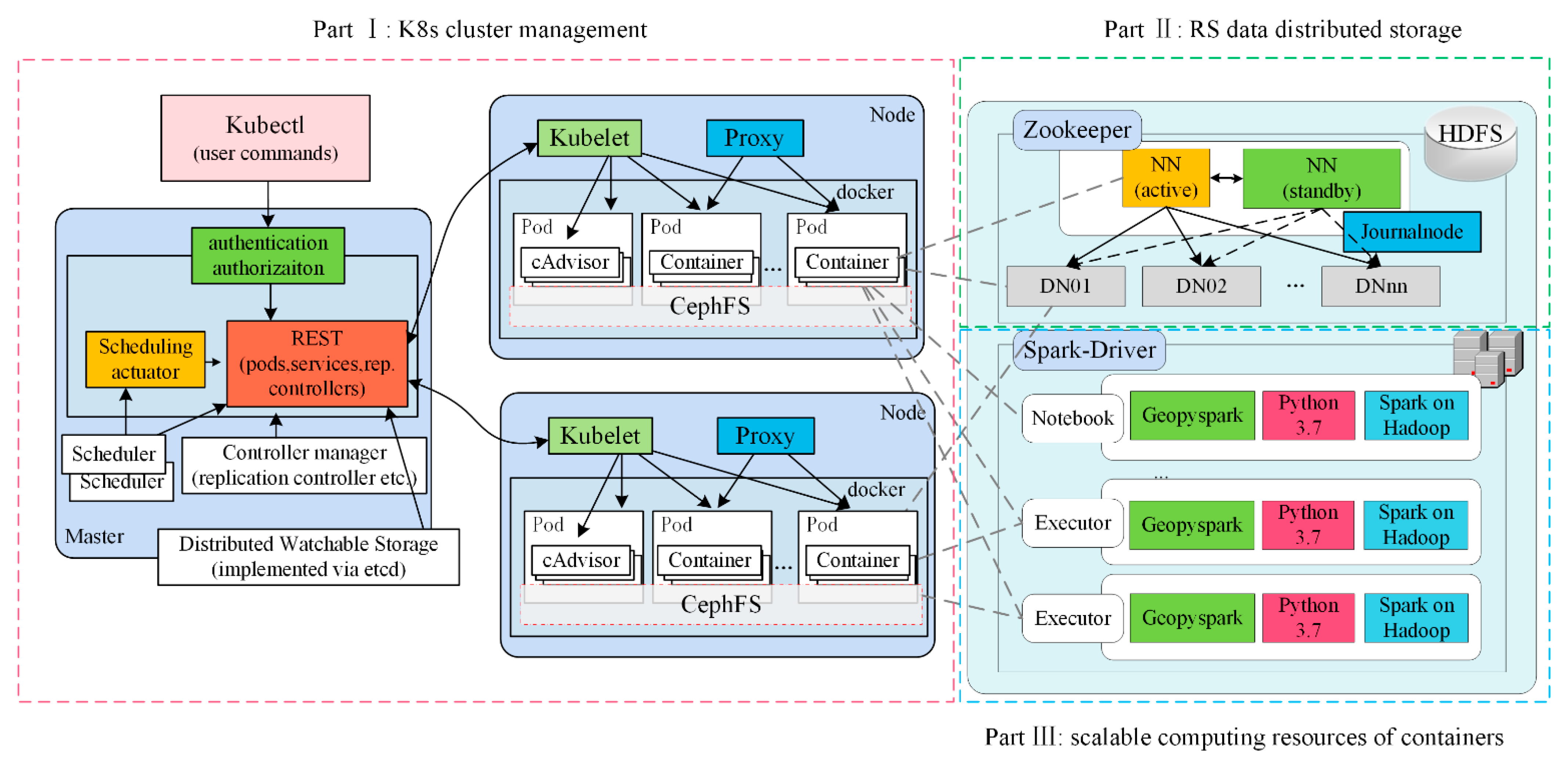
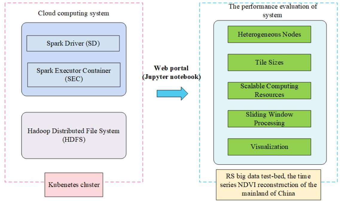
2.2. The Ditributed Parallel Architecture of System

The architecture of the proposed scalable computing resources system is illustrated in Figure 1. The system consists of three parts, namely, K8s cluster management (Part I), RS data distributed storage (Part II), and scalable computing resources of the containers (Part III). All nodes contained in this big data framework act as both computing nodes and storage nodes to avoid data movement between computing nodes.
The K8s cluster management (Part I) is mainly responsible for resource management, user authentication, service accounting, and configuration management. K8s was selected as the container orchestration platform based on its widespread adoption in the market and the fact that it has become a recognized container orchestration standard [16]. As the foundation of the K8s cluster, CephFS [46] was implemented on low-level nodes to provide a storage-class [47] for the PersistentVolume [48] of K8s. This improves the robustness of the K8s cluster by enabling other running nodes to take over the services provided by nodes that are down. Using Kuboard, a free-use management tool of K8s, users can easily control and monitor the use of hardware, such as CPU, storage, and RAM.
The RS data distributed storage (Part III) is the infrastructure for storing huge RS datasets. In this part, we implemented HDFS on the K8s cluster. To ensure the high availability of the storage system, we deployed two NameNodes (NNs)—one in active status, and the other in standby status—to ensure the high availability of HDFS. The NameNode (NN) is the centerpiece of an HDFS file system. It keeps the directory tree of all files in the file system and tracks where the file data is kept across the cluster. It does not store the data of these files itself. The DataNode (DN) is responsible for storing the actual data in HDFS. In our platform, DataNodes (DNs) are distributed in all VMNs to reduce data movement between nodes. HDFS [49] is a popular cloud storage platform and streaming data access pattern, which can store huge, distributed file datasets, and write once and read many times. It is especially suitable for deployment on lower-cost computers consisting of a cluster because of its high reliability and high-performance characteristics. Therefore, we choose HDFS for data storage due to its outstanding capacity and high-speed read throughput of RS big data [50].
The scalable computing resources of containers (Part III) consists of a Spark driver container with a Jupyter notebook and Spark executor containers. At the core, K8s with containerized Spark is integrated in the system to realize the assignment of scalable computing resources. In our system, we initialize a Spark application by only providing hints about the memory allocation to Spark Driver (SD). The parameters of Spark Executor Container (SEC), such as the number of instances, vcores, and memory, can be dynamically adjusted in each Spark application due to the fast initialization of containerized Spark by the Jupyter notebook console.
All of these containers are created by Docker images, which contain a series of Python libraries for raster data processing. The Jupyter notebook extends the console-based approach to interactive computing, which is a qualitatively new direction. It provides a web-based application suitable for capturing the whole computation process, including developing, documenting, and executing code, in addition to communicating the results. GeoPySpark [42] is a Python language binding library of GeoTrellis. GeoTrellis [51] is a geographic data processing engine for high performance applications, which provides data types for working with raster in the Scala language, in addition to a number of operations to manipulate raster data. GeoPySpark utilizes GeoTrellis to allow reading, writing, and operating of raster data. In GeoPySpark, raster images are represented by the tile class, which contains a NumPy array to represent the raster cells and other information regarding the data.
The computing containers are implemented based on Python-3.7.3 and integrated with a Jupyter notebook as the access interface between the system and user-clients. As an indispensable part of the system, we integrated the mainstream Matplotlib [52] package of the Python library for data visualization, which is a comprehensive library for creating static, animated, and interactive visualization in Python. This enables publication-quality figures to be generated in a variety of hardcopy formats and interactive environments across platforms. When installing the Jupyter notebook application using Helm tools [53] in the K8s cluster, three services for running notebook container need to be deployed, namely, the web browser service, Spark driver service, and Spark UI service. The web browser service is exposed through haproxy-ingress [54] to provide a highly available and accessible service to client-side users.
The SparkContext is the entry point to any Spark functionality. When a Spark application is run, a driver program is hosted, which has the main function and imitates the SparkContext. The driver program then runs operations inside the executors on the worker nodes. Only two steps are needed to initialize a new SparkContext: (1) import the Python core libraries of GeoPySpark; (2) configure the parameters and create SparkContext. After creating a new SparkContext, computing jobs can easily be submitted to the cluster through the console cell. In our hundreds of executions, we used the Jupyter notebook as the user interface, which can provide a convenient way to adjust the parameters of Spark executors in the K8s cluster. In the parameter configuration section, we can configure the numbers of executors by defining the parameters of spark.executor.instances, the CPU cores of executors by spark.executor.cores, and each memory size of executors by spark.executor.memory. It is worth noting that the number of tasks is determined by the numbers of executors and vcores, which is equal to the product of the executors and vcores count. The Spark driver service is used to create scalable computing resources for the Spark executors by configuring the three above-mentioned parameters of SparkContext in the K8s cluster. Spark UI is exploited to monitor the running status of multiple tasks submitted by client users.

2.3. The Design of Experiments

In order to scientifically evaluate the factors that affect the performance of the system, we utilized one of the most widely used RS vegetation indices—Normalized Difference Vegetation Index (NDVI)—as a testbed to evaluate the feasibility and performance of our system. NDVI is one of the main vegetation indexes reflecting the spectral characteristics of vegetation [55]. It has been widely applied in various fields, such as environment monitoring systems on global or regional scales, analyzing vegetation and land cover dynamics, and extracting information of vegetation phenology [56]. In this work, to avoid more data movement in cluster nodes, we built HDFS storage on the heterogenous nodes, which are also Spark computing workers. In this study, we further explored how the less powerful nodes affect the efficiency of the whole cluster, which is crucial to build a data-intensive parallel computing system. In addition, when using GeoPySpark as the data processing library, it is necessary to carefully study the effect of tile size on tiling, computing, and writing. For raster data with the same computational complexity and size, a good question to guide the allocation of scientific resources is whether extending the computing resources can accelerate the computing progress. Finally, as the system is mainly used to analyze RS data, visualization provides an intuitive presentation for users to quickly understand the information in multiple scales.

2.4. The Data Sources of Experiments

To prove the feasibility and robust of the system, three experiments were performed. Moderate Resolution Imaging Spectroradiometer (MODIS) daily series images were analyzed and processed using the proposed system. MODIS is a key instrument onboard Terra (originally known as EOS AM-1) and Aqua (originally known as EOS PM-1) satellites. Terra MODIS and Aqua MODIS view the entire Earth’s surface every 1 to 2 days. Thus, the MODIS sensor is suitable for some daily surface monitoring applications such as monitoring vegetation change. Nevertheless, the reflectance bands receive radiation from the cloud layer rather than the land surface due to the cloud effect. Therefore, it is also necessary to solve the problem of discontinuities in temporal and spatial data caused by cloud pollution in the vegetation change application.
In our experiments, we utilized two products of MODIS, MOD09GQ, and MOD35. MOD09GQ [57] provides MODIS band 1–2 daily surface reflectance at 250 m resolution. The MODIS cloud mask (MOD35) [58] is a science data product. It is regularly produced as a standard product of the Earth Observing System (EOS). Its main purpose is to identify scenes where land, ocean, and atmosphere products should be retrieved based upon the amount of obstruction of the surface due to clouds and thick aerosol.
The MODIS NDVI [59] can be calculated by using the surface reflectance of MODIS red and near infrared bands according to:
N D V I = N I R R E D N I R + R E D
where NIR is the near-infrared band and RED is the red band of MOD09GQ products. The production process of MODIS NDVI is illustrated in Figure 2, and mainly includes Cloud Mask (CM), image preprocessing, Quality Control (QC), and vegetation index calculation.
The whole of mainland China was selected as the study area, and the daily NDVI dataset with 250 m spatial resolution and long time series (from 2002 to 2020) was produced by utilizing the proposed scalable computing resources big data system. The production process of the daily NDVI dataset produces almost 2GB of raster data per day, in which the data volume of the MOD35 cloud mask is approximately 332 MB; each quality assessment, for red and near-infrared bands, is almost 665 MB. The whole of mainland China has 24,642 × 14,157 pixels in a spatial resolution of 250 m (approximately 0.0025°). The daily NDVI is stored in HDFS format as an individual catalog, with metadata of the TiledRasterLayer stored separately as a json file. The file stored as a catalog can be easily used to explore data of different scales, such as a point, a square, or any defined box. Map algebra operations are provided by GeoPySpark. Local and focal operations are performed only on the TiledRasterLayer. Therefore, we need transform the RasterLayer to the TiledRasterLayer before any operations can be loaded in raster data. As the tiled format is stored in a catalog, we can explore time-series data information at a point or a local regional area.

2.5. Time Cost of Compurting Mechanism

In this distributed parallel system, the time cost for the complete process for calculation contains three parts, namely, data load time (denoted as TL), computing time (denoted as TC), and collecting and writing time (denoted as TW). The total processing time Ttotal of the band-oriented RS algorithm can be formulated as following:
T t o t a l = T L + T C + T W
Not only does TL depend on the I/O rates of the hard disk, but it also relates to the volume of data moving among the nodes. TC is determined by the tile size (STILE), the tiling numbers of the raster layer (denoted as NTILE), the number of SECs (denoted as NSEC), and the vcores of each SEC (denoted as VSEC). Hence, the TC can be represented as Equation (3). Equation (3) clearly shows that the larger NSEC and VSEC, the lower the value of TC.
T C = N T I L E × S T I L E N S E C × V S E C
If a raster layer’s columns and rows are represented by Ncols and Nrows, respectively, NTILE can be expressed as Equation (4). Thus, the smaller STILE, the more tiles will be generated.
N T I L E = ( N c o l s / S T I L E + 1 ) × ( N r o w s / S T I L E + 1 )
TW is mainly decided by the tiling numbers of the raster layer (NTILE), the number of SECs (NSEC), and the vcores of each SEC (VSEC). The bigger the value of NTILE, the greater the cost of the collecting time. The greater the values of NSEC and VSEC, the more resources needed by SD to maintain the status of all SECs, which affects the writing time of the calculation result.
The above explanation indicates that TC and TW contradict each other. Therefore, when designing an algorithm for RS datasets, the complexity of the algorithm should be considered. If the computing is intensive, such as in time series data construction, more SEC instances and bigger vcores should be initialized. Otherwise, fewer resources should be applied, thus allowing more resources to be provided to other data processes.

3. System Environment

The experimental environment consists of six virtual machine nodes. We used the HUAWEI FusionCompute virtualization cloud platform to create these VMNs; four of these were hosted on the FusionComputeV100R006 platform (R006), and two on the V100R005 platform (R005). The physical servers in R006 have Intel(R) Xeon(R) CPU E5-2630 v4 @ 2.20 GHz, Intel Corporation 82599EB 10 Gigabit Dual Port Backplane Connection (network), and 128GB memory on the V100R006 platform. The R005 servers have Intel(R) Xeon(R) CPU E5-2620 v2 @ 2.10 GHz, Intel Corporation I350 Gigabit Network Connection(network), and 64GB memory. Thus, the physical servers in R005 possess a less powerful CPU and slower network rate than those in R006. The hardware configurations of the VMNs in the K8s cluster are listed in Table 1. In total, there were 48 vcores and 144GB memory available in the system.
To monitor cluster performance, the Kuboard and Spark job monitor were used. The operating system (OS) of all nodes was Centos-7.4-x86_64. Docker was selected to provide the container execution environment due to its tight integration with K8s and wide industry adoption [60]. The software of the VMN and Docker images used in the platform is listed in Table 2. To manage the container-based workloads, our container-based orchestration platform consists of six nodes, namely, one master node and five worker nodes in the K8s cluster. It can be seen that our system is heterogeneous with different hardware and different networks.
We built spark-notebook and spark-py Docker images from the openjdk:8-jdk-slim base layer for processing RS data; the packages integrated in each of images are listed in Table 3. The spark-notebook image and the spark-py image was used to create the Spark driver container and Spark executor containers, respectively. These images were pushed to registry.cn-hangzhou.aliyuncs.com [61] (accessed on 28 November 2021) as a public repository. These images can be accessed by any users who wish to analyze RS images using container-oriented programming.

4. Results

We evaluated the performance of the system through a case study in which the daily distribution of 250 m NDVI within the mainland area of China was estimated using MODIS surface reflectance and cloud product data. Below, we first discuss the efficiency of heterogeneous nodes, and analyze the impact of the tile size. We then evaluate the efficiency of submitting computing jobs with different computing resources, and finally explore how to mine time-series information more effectively from massive amounts of RS data with a given tile size.

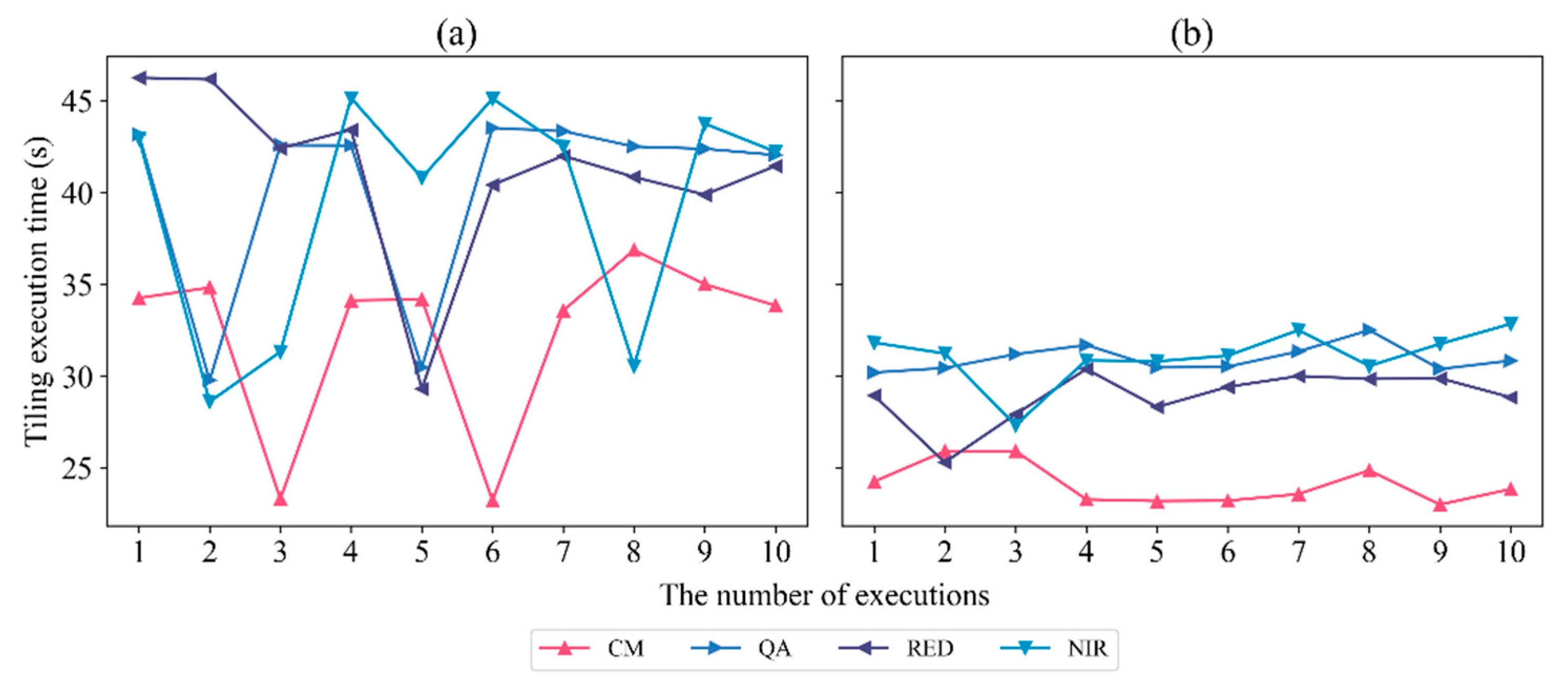
4.1. Time Cost of Heterogeneous Nodes

In order to evaluate the impact of the less powerful nodes on the performance of the cluster, we tracked the detailed time cost of the multi-task stages of the tiling job through the Spark UI service. We initialized a SparkContext and parameterized six executors with 8 GB memory and 2 vcores in this experiment. We executed the containerized Spark application twenty times and recorded each tiling execution time. All computing nodes were used in the first ten executions, and less powerful nodes were disabled in the final ten executions. As shown in Figure 3, when scheduling all nodes in the K8s cluster, some jobs were inevitably submitted to the less powerful nodes (node5 and node6), and the time cost of tiling varied (Figure 3a). When the less powerful nodes were disabled from scheduling, all executors were initialized in the efficient nodes, and the time cost of tiling was more stable. Taking the execution time of CM data processing process as an example, the highest time cost was over 35 s when the less powerful nodes were included in the computing stages. However, the time cost reduced to 22 s when the less powerful noes were disabled. It should be noted that the time costs of some executions were close to 25 s. The reason for this is that the datasets were stored and computed in different VMNs by tracking the details of the Spark UI service and the HDFS management system. The maximum performance gain was up to 37.1% ((35–22)/35).

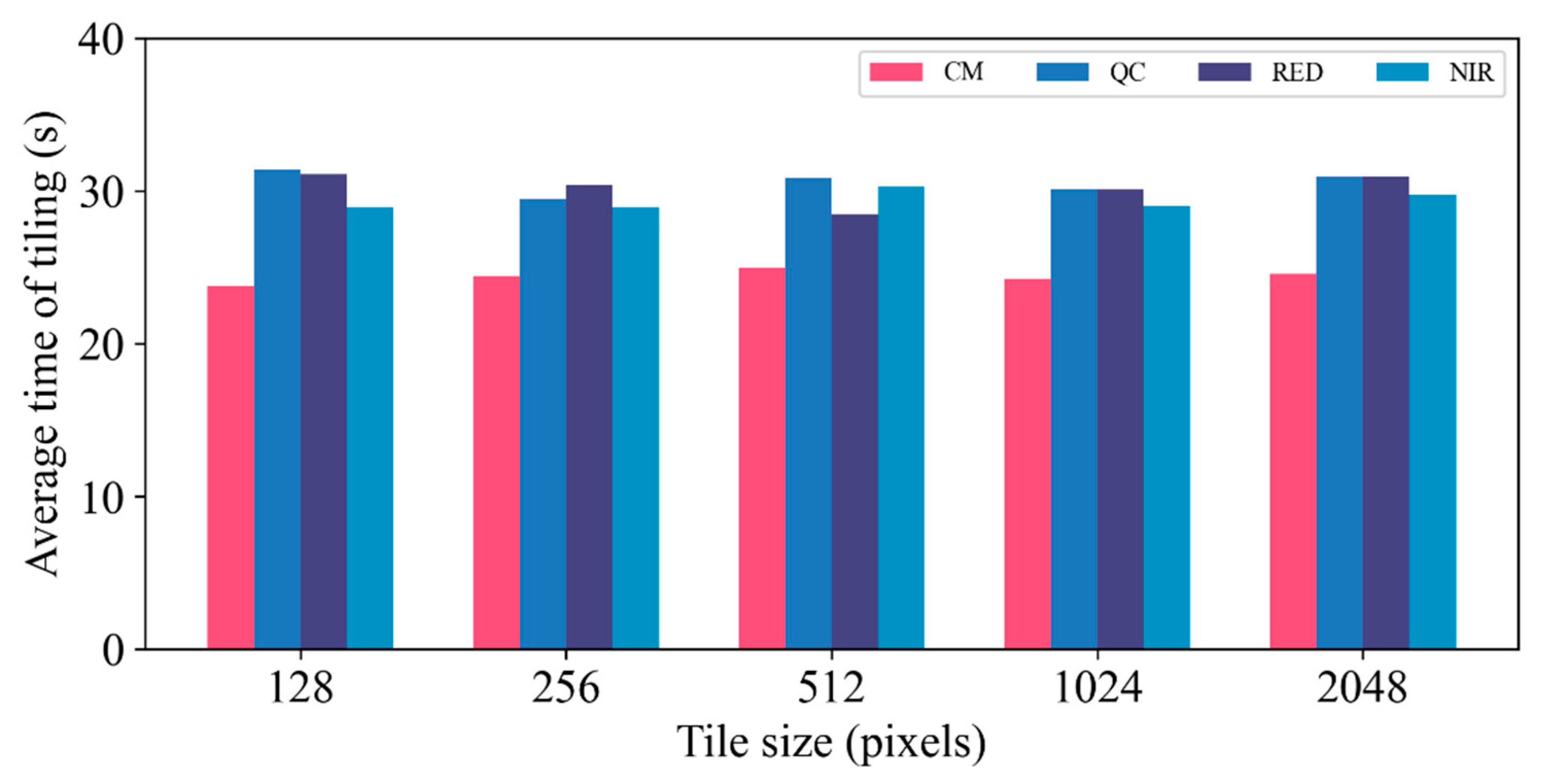
4.2. Time Cost in Different Tile Sizes

Because all map algebra operations only work on the TiledRasterLayer, each raster band file needs to be tiled as a TiledRasterLayer after it is loaded as a RasterLayer. Therefore, it is necessary to study the effect of tile size on the efficiency of raster layers’ processing. We produced the NDVI in the SparkContext, using six executors, two cores, and 8GB memory. Each given tile size experiment was executed 10 times, and the average execution time of the tiling stages and computing-writing stages were recorded separately. As shown in Figure 4, the average tiling time for different tile sizes was almost the same. Each smaller raster file (i.e., CM data) took 25 s, whereas each larger file (i.e., QC, RED, and NIR data) took almost 30 s under different tile sizes. Therefore, the tile size is not a prominent factor related to the time cost of the tiling stage, when each procedure is in the same SparkContext configuration.
Spark has lazy loading behavior for transformations, which means that it does not trigger the computation of the transformation. Rather, it only tracks the requested transformation. When a user writes a transformation to obtain another dataset from an input dataset, it can be written in a way that makes the code readable. Therefore, we further explored the time cost of the computing-writing stage.
We tracked the detailed time cost in the Spark UI monitor service and found that the size of the tile is the main factor affecting the computing-writing efficiency of the cluster, as shown in Figure 5. The time cost of computing-writing increases almost with the size of tile. The minimum time cost occurred in the second execution when the tile size was 256 pixels, and the maximum time cost appeared in the fourth execution then the tile size was 2048 pixels. The minimum time cost occurred in the case of a smaller tile size, but this does not mean that a smaller tile size is better in computing-writing stages, and the tile size of 512 pixels had a more stable time cost than other tile sizes.

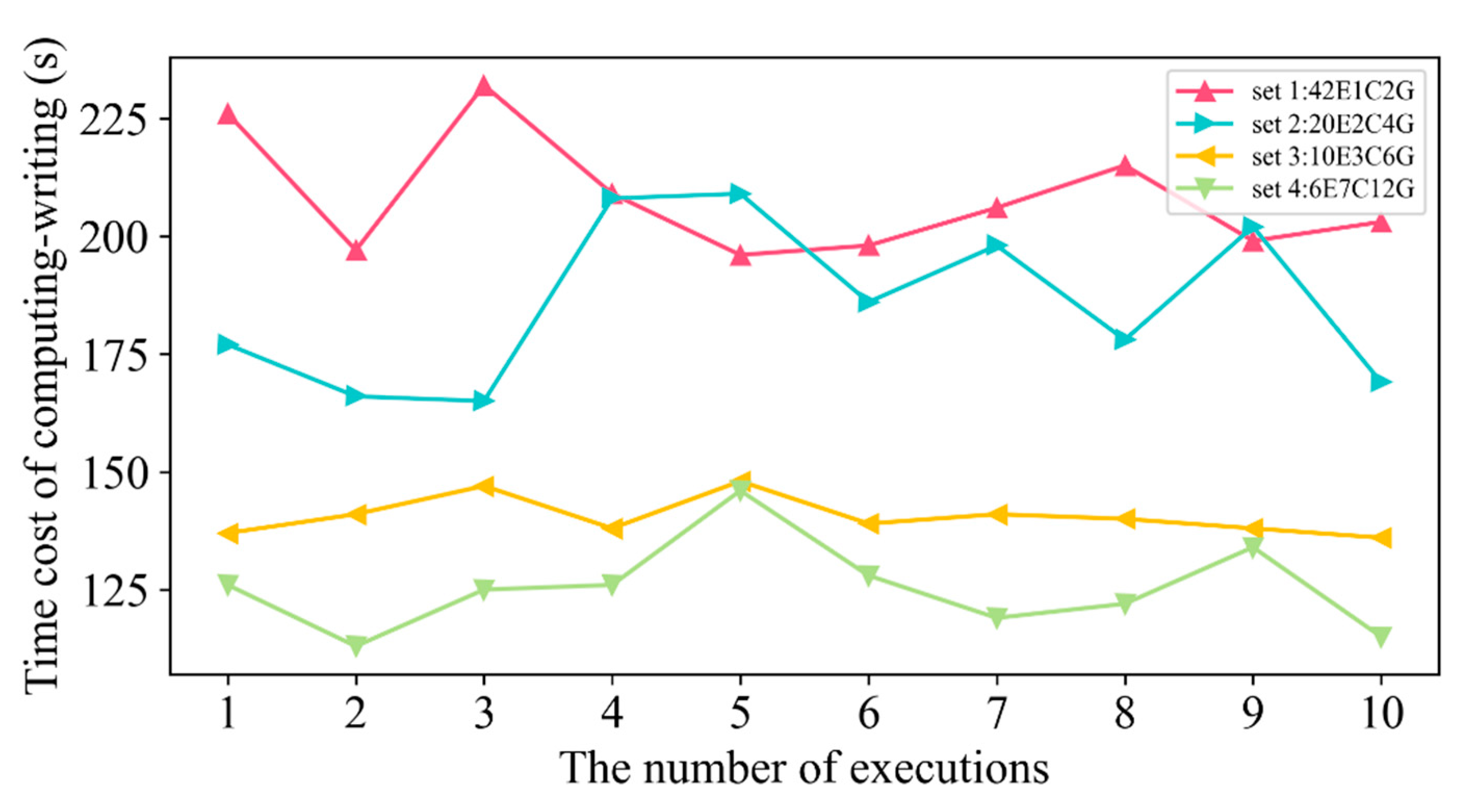
4.3. Time Cost of Scalable Computing Resources

As mentioned in Section 3, the system we implemented possesses 48 vcores and 144GB memory. All data required for processing were concentrated in one place and closely coupled with the processing resources to guarantee efficient development and convenient access. All nodes were used not only for distributed storage of data, but also for data processing. All these resources were used for the OS, K8s management, HDFS on K8s, and computing. Thus, the computing resources that we can lease must not include the resources occupied by the OS, K8s cluster management, and HDFS. Hence, nearly 42 vcores and 100GB memory resources monitored by Kuboard can be leased for computing. According to official documents relating to Spark performance tuning [62], the numbers of executors and cores, and the executor memory, are the three main factors that may affect the performance of Spark-based applications.
In this study, four different configuration sets were designed as follows: (1) 42 executors with 2GB memory and one vcore each as set 1 (42E1C2G); (2) 20 executors with 4GB memory and two vcores each as set 2 (20E2C4G); (3) 10 executors with 6GB memory and three vcores as set 3 (10E3C6G); and (4) six executors with 12GB memory and seven vcores as set 4 (6E7C12G). These four configuration sets can use almost all the computing vcores and free memory of the cluster, but are unable to fully use all of the computing vcores and free memory. For example, we can theoretically assign 10 executors with 8GB memory and four vcores in set 3. This is because nodes 3, 5, and 6 only have a total of eight vcores and 16 GB memory. As mentioned above, some resources must be kept for the basic running of the cluster, such as OS, cluster manager, and HDFS. Therefore, if two executors with 8GB memory and four vcores use resources on one node, nodes 3, 4, or 5, for example, will not have enough resources to lease. Thus, it is worth noting that when designing a Spark on K8s cluster with HDFS, the computing vcores and memory should be as large as the physical machine resources to avoid the waste of resources.
In computing-writing jobs of the daily NDVI calculation, four flatMap stages, three RDD collect stages, and one RDDWriter stage are included. RDD collect and RDDWriter stages result in slow progress, which increases the time cost of the Spark computing framework. The time cost of computing-writing jobs under four different configuration sets (512-pixel tile size) are shown in Figure 6. We found that the time cost increases with the increase in the number of executors under the same algorithm complexity.

4.4. Time Cost of Sliding Window Processing

To investigate the performance of the system in spatial computation for RS big data, the Sliding Window Algorithm (SWA) was selected for this study. Focal operations, including MEAN, MEDIAN, MODE, SUM, STANDARD_DEVIATION, MIN, MAX, SLOPE, and ASPECT, were performed in GeoPySpark by executing a given operation on a neighborhood throughout each tile in the layer. We chose the MEAN operation and an int16 data type of the TiledRasterLayer in the 3 × 3, 5 × 5, 7 × 7, and 9 × 9 sliding windows (SWs) under the three different computing resources, namely, 20 executors with 4GB memory and two vcores (20E2C4G), 10 executors with 4GB memory and two vcores (10E2C4G), and five executors with 4GB memory and two vcores (5E2C4G). Each given SW experiment was executed five times, and the execution time of processing was recorded, as shown in Figure 7(a1–a3). We also repeated all the tests in a float32 data type of the TiledRasterLayer in different SWs, as illustrated in Figure 7(b1–b3). The int16 and float32 data type of the raster layer had the same grid size and resolution. The results illustrate that the average time costs of the float32 data type are higher than those of the int16 data type by about 9.2 s (58.625–49.42), 4.35 s (59.27–54.92), and 4.25 s (59.74–55.49) in all sliding window executions under the configurations of 20E2C4G, 10E2C4G, and 5E2C4G, respectively. The efficiency of computing-writing is little affected by the size of the SW in the parallel computing paradigm under the same computing resources.

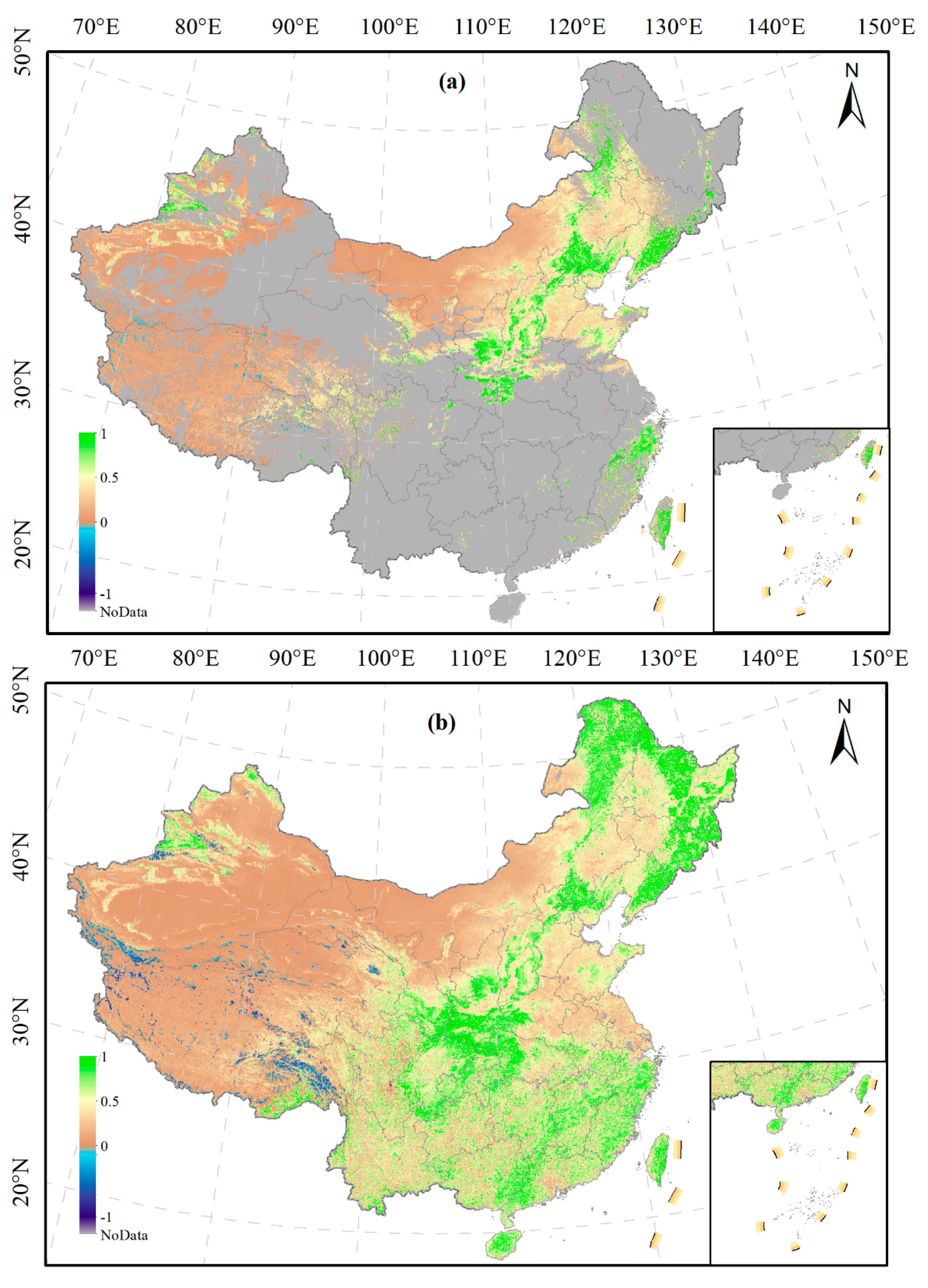
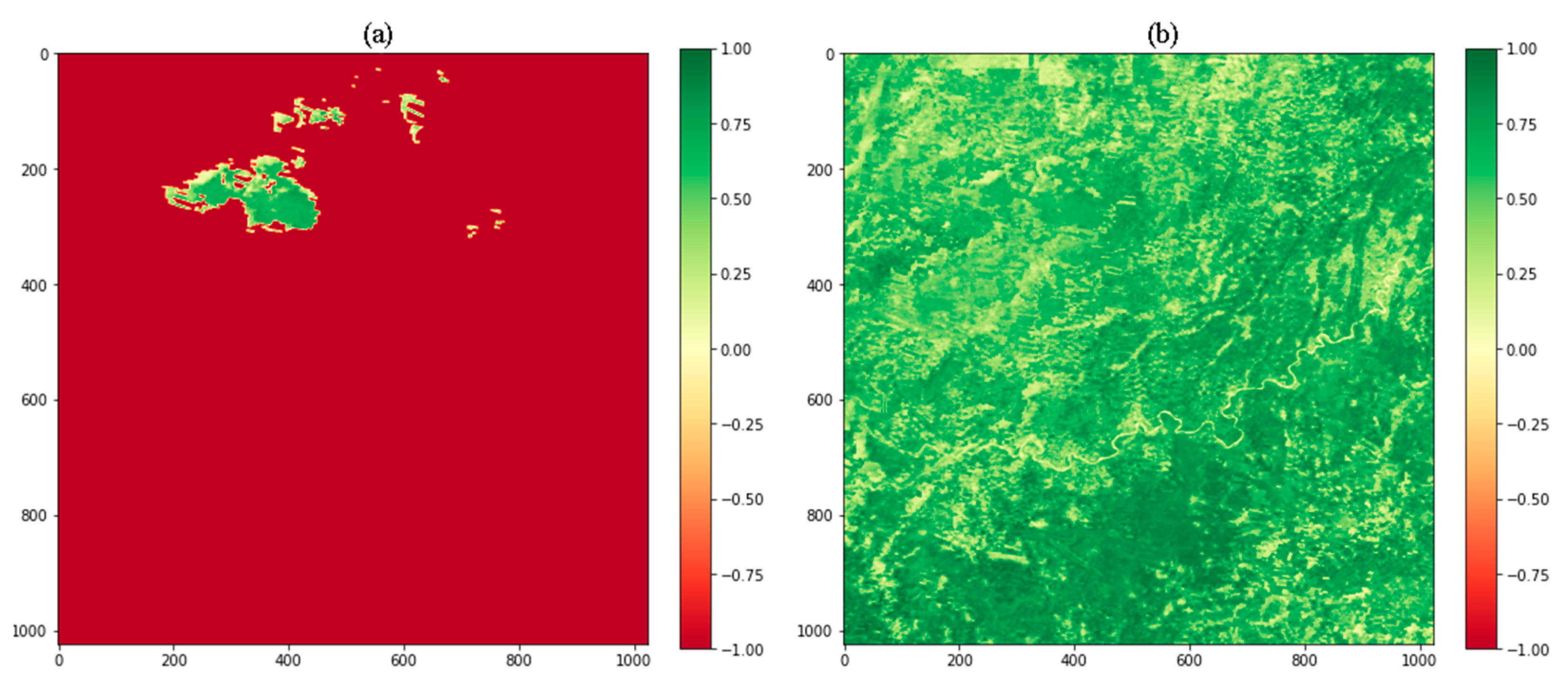
4.5. Multi-Scale Visualization

In this work, we used the GeoPySpark raster data processing package, which can easily obtain information from the TiledRasterLayer catalog at a point or for any defined box scale. We took the visualization of the NDVI calculation results on 14 June 2020 as an example. The NDVI distribution in the whole study area and the specified tile scale (e.g., a tile having a size of 1024 × 1024 pixels) can be easily visualized in the system, as shown in Figure 8 and Figure 9. Therefore, our system can be used to easily view and visualize the multi-scale information relevant to users through the user interface of the web browser.

5. Discussion

The results of this study indicate that the tile-oriented programming model can easily implement parallel computing of RS big data without destroying the spatial structure of the raster data. The raster layers can be abstracted as many small-size tiles, and a computing task can be divided into many small tile computing tasks, which can be assigned scalable computing resources (SEC). To investigate the factors that affect the efficiency of the system, we carried out several experiments after considering the hardware and computing paradigm. As a result, we found that the tile size plays an important role in parallel computing. When the tile size became smaller, the time cost was shorter. This is because the greater number of tiles generated can completely utilize the distributed computing resources. However, this does not mean the smaller tile size is better, and the stable time costs appear at a tile size of 512 pixels. The reason for this is that more time is spent on the counting of the HadoopRDDWriter (Resilient Distributed Dataset, RDD) stage for smaller size tiles, and on the flatMap operation of CutTiles stages for larger size tiles. Therefore, the size of the tile portion should not be too small or too big. Our experiments obtained results that were similar to those of previous studies [18,21], but there were still some divergences.
The computing resources is another vital factor that influences the computing efficiency. The number of computing tasks is decided by the number of vcores of SECs. For a simple computing complexity, the greater the number of containers that are leased, the more the driver manager will maintain the computing status of all executors and the greater the data movement in the shuffle progress. Therefore, a larger number of vcores of executors does not provide better results. Due to the implementation of the HDFS storage in the K8s computing nodes, the time costs are slightly inconsistent under the same computing resources, complexity of algorithm, and tile size because of the RS images stored in the same computing nodes.
The complexity of RS data processing algorithms also affects the performance of the computing-writing stage. The average time cost of a band-wise algorithm such as the NDVI algorithm was 187 s under 20E2C4G computing resources, and the average time cost of SW was nearly 50 s under the same computing resources. Because the NDVI algorithm contains four raster bands, the time cost of each band was almost 47 s. Thus, we found that the complex algorithm of spatial computing needs more time than the simple band-wise algorithm, but the difference was not as obvious in the parallel computing paradigm.
The data type is also a factor that can have a considerable effect on the computational time cost and storage space. The storage space of the RS layer having the same grid will double in float32 and quadruple in float64 compared with the int16 data type. Similarly, the computing time will increase when the NDVI value is converted from int16 into the float32 data type by expanding 10,000 times and rounding as an integer. Therefore, the data type may be transformed from float to integer to improve the computing performance and to save storage space when the accuracy of processing result is not (or is slightly) affected within an acceptable range.
The hardware of the physical servers may have an effect on the system. A server with stronger CPU rate will speed up a computing task, and a weaker CPU will slow the task. Therefore, we built the system on several nodes virtualized in heterogeneous physical servers. In this case, the less powerful nodes reduce the efficiency of the cluster, as in the case of the “Cask Effect”, and any shortage affects the efficiency of the whole cluster. This also indicates that all computing tasks are balance loaded in distributed SECs according to the task scheduling mechanism of Spark on K8s.

6. Conclusions

In this study, we explored the state-of-the-art technologies for analysis and processing of RS big data, such as the storage, computing, and visualization of massive raster datasets generated from EOS. To improve the overall efficiency of the system, we adopted several novelty technological strategies. At the stage of loading data, we used HDFS on K8s architecture to avoid a huge volume of RS data movement in computing nodes. Hence, the time cost during the RS data storage is lower in the same node with computing nodes. Although the homogeneous physical server in a whole cluster is very effective, the distributed parallel platforms are usually built on several existing heterogenous servers. At the stage of computing, when the tasks were scheduled in the clusters excluding less powerful nodes, the time cost of the computing-writing stage was more stable. In our system, as mentioned in Section 3, the less powerful nodes hosted by the R005 platform are connected in the platform through a less powerful network. Therefore, the performance of the cluster is lower in the collecting and shuffling operations with huge data transmission among the nodes. Moreover, the tile-oriented programing model is quite efficient for large scales of the RS raster layer. The tile size is a crucial factor that affects the time cost in the computing-writing stages, and tiles cannot be too big or too small. Tiles that are too big cannot completely utilize the parallel computing resources, whereas tiles that are too small need more time to collect the results. The number and vcores of SECs are another key factor that has an impact on the capability in the computing-writing stages. For the band-oriented RS algorithm, such as the NDVI calculation, the complexity of computing is not highly intensive; therefore, increasing the computing resources does not improve the performance. Additionally, we assembled flexible packages of Python in Docker images, such as GDAL, GeoPySpark, and Matplotlib, which provided a convenient environment for RS data analysis and visualization at multiple scales. Therefore, we believe that the system proposed in this study can be easily transplanted to other big data platforms, such as AWS, Azure, Google GCP, Aliyun, and Tencent Cloud, based on open-access Docker images pushed to a public repository. In summary, the system we explored is clearly suitable for RS big data processing.
This work also has some shortcomings that will need to be addressed in the future. Our future work will investigate these issues, such as developing a multi-user analysis system for RS big data, upscaling or downscaling RS data pre-processing based on the pyramid class in GeoPySpark, and providing a cloud Tile Map Service (TMS) directly from both GeoPySpark RDDs and the tile catalog.

Author Contributions

Conceptualization, J.G. and J.H.; methodology, J.G.; software, J.G.; validation, J.G., J.H. and C.H.; formal analysis, J.G.; investigation, J.H.; resources, C.H.; data curation, J.G.; writing—original draft preparation, J.G.; writing—review and editing, J.G. and J.H.; visualization, J.G.; supervision, C.H.; project administration, J.G.; funding acquisition, C.H. All authors have read and agreed to the published version of the manuscript.

Funding

This research was funded in part by National Natural Science Foundation of China, grant number 42130113; in part by Strategic Priority Research Program of the Chinese Academy of Sciences “CAS Earth Big Data Science Project”, grant number XDA19040504; and in part by the Basic Research Innovative Groups of Gansu province, China, grant number 21JR7RA068.

Institutional Review Board Statement

Not applicable.

Informed Consent Statement

Not applicable.

Data Availability Statement

The Docker images of the Jupyter notebook and the pyspark executor in this study are available online from registry.cn-hangzhou.aliyuncs.com/guojf/spark-notebook:rf-geopyspark-pyproj [61] and registry.cn-hangzhou.aliyuncs.com/guojf/spark-py:geopyspark [61], respectively. (accessed on 28 November 2021).

Acknowledgments

We are grateful to LocationTech Labs, who provided the GeoPySpark library for this research. We would also like to thank NASA, who provided Cuprite data for the experimental validation.

Conflicts of Interest

The authors declare no conflict of interest.

Abbreviations

The following abbreviations are used in this manuscript:
CMCloud Mask
DNDataNode of HDFS
DPCDistributed Parallel Computing
EOEarth Observation
EOSEarth Observing System
FOSSFree and Open-Source Software
GDALGeospatial Data Abstraction Library
GEEGoogle Earth Engine
HDFSHadoop Distributed File System
HPCHigh-Performance Computing
JEODPPJRC Earth Observation Data and Processing Platform
JRCJoint Research Center
LXCLinux Container
MODISModerate Resolution Imaging Spectroradiometer
NDVINormalized Difference Vegetation Index
NNNameNode of HDFS
ODCOpen Data Cube
QCQuality Control
RDDResilient Distributed Datasets
SDSpark Driver
SECSpark Executor Containers
SEPALSystem for Earth Observation Data Access, Processing and Analysis for Land Monitoring
SHSentinel Hub
VMNVirtual Machine Node
VMsVirtual Machines
YARNYet Another Resource Negotiator

References

  1. Deren, L.; Liangpei, Z.; Guisong, X. Automatic analysis and mining of remote sensing big data. Acta Geod. Cartogr. Sin. 2014, 43, 1211. [Google Scholar]
  2. Ma, Y.; Wu, H.; Wang, L.; Huang, B.; Ranjan, R.; Zomaya, A.; Jie, W. Remote sensing big data computing: Challenges and opportunities. Future Gener. Comput. Syst. 2015, 51, 47–60. [Google Scholar] [CrossRef] [Green Version]
  3. Skytland, N. Big data: What is nasa doing with big data today. Open. Gov. Open Access Artic. 2012. Available online: https://www.opennasa.org/what-is-nasa-doing-with-big-data-today.html (accessed on 28 November 2021).
  4. Gamba, P.; Du, P.; Juergens, C.; Maktav, D. Foreword to the special issue on “human settlements: A global remote sensing challenge”. IEEE J. Sel. Top. Appl. Earth Obs. Remote Sens. 2011, 4, 5–7. [Google Scholar] [CrossRef]
  5. Stromann, O.; Nascetti, A.; Yousif, O.; Ban, Y. Dimensionality Reduction and Feature Selection for Object-Based Land Cover Classification based on Sentinel-1 and Sentinel-2 Time Series Using Google Earth Engine. Remote Sens. 2020, 12, 76. [Google Scholar] [CrossRef] [Green Version]
  6. Müller, M.; Bernard, L.; Brauner, J. Moving code in spatial data infrastructures–web service based deployment of geoprocessing algorithms. Trans. GIS 2010, 14, 101–118. [Google Scholar] [CrossRef]
  7. Camara, G.; Assis, L.F.; Ribeiro, G.; Ferreira, K.R.; Llapa, E.; Vinhas, L. Big earth observation data analytics: Matching requirements to system architectures. In Proceedings of the 5th ACM SIGSPATIAL International Workshop on Analytics for Big Geospatial Data, Burlingame, CA, USA, 31 October 2016; pp. 1–6. [Google Scholar]
  8. Gomes, V.C.F.; Queiroz, G.R.; Ferreira, K.R. An Overview of Platforms for Big Earth Observation Data Management and Analysis. Remote Sens. 2020, 12, 1253. [Google Scholar] [CrossRef] [Green Version]
  9. Mell, P.; Grance, T. The NIST Definition of Cloud Computing; National Institute of Standards and Technology: Gaithersburg, MD, USA, 2011.
  10. Mutanga, O.; Kumar, L. Google Earth Engine Applications. Remote Sens. 2019, 11, 591. [Google Scholar] [CrossRef] [Green Version]
  11. White, T. Hadoop: The Definitive Guide; O’Reilly Media, Inc.: Newton, MD, USA, 2012. [Google Scholar]
  12. Jo, J.; Lee, K.-W. High-performance geospatial big data processing system based on MapReduce. ISPRS Int. J. Geo-Inf. 2018, 7, 399. [Google Scholar] [CrossRef] [Green Version]
  13. Cary, A.; Sun, Z.; Hristidis, V.; Rishe, N. Experiences on processing spatial data with mapreduce. In Proceedings of the International Conference on Scientific and Statistical Database Management, New Orleans, LA, USA, 2–4 June 2009; pp. 302–319. [Google Scholar]
  14. Eldawy, A.; Mokbel, M.F. A demonstration of spatialhadoop: An efficient mapreduce framework for spatial data. Proc. VLDB Endow. 2013, 6, 1230–1233. [Google Scholar] [CrossRef] [Green Version]
  15. Giachetta, R. A framework for processing large scale geospatial and remote sensing data in MapReduce environment. Comput. Graph. 2015, 49, 37–46. [Google Scholar] [CrossRef]
  16. Aji, A.; Wang, F.; Vo, H.; Lee, R.; Liu, Q.; Zhang, X.; Saltz, J. Hadoop-GIS: A high performance spatial data warehousing system over MapReduce. In Proceedings of the VLDB Endowment International Conference on Very Large Data Bases, Trento, Italy, 26–30 August 2013. [Google Scholar]
  17. Quirita, V.A.A.; da Costa, G.A.O.P.; Happ, P.N.; Feitosa, R.Q.; da Silva Ferreira, R.; Oliveira, D.A.B.; Plaza, A. A new cloud computing architecture for the classification of remote sensing data. IEEE J. Sel. Top. Appl. Earth Obs. Remote Sens. 2016, 10, 409–416. [Google Scholar] [CrossRef]
  18. Huang, W.; Meng, L.; Zhang, D.; Zhang, W. In-memory parallel processing of massive remotely sensed data using an apache spark on hadoop yarn model. IEEE J. Sel. Top. Appl. Earth Obs. Remote Sens. 2016, 10, 3–19. [Google Scholar] [CrossRef]
  19. Wang, L.; Ma, Y.; Yan, J.; Chang, V.; Zomaya, A.Y. pipsCloud: High performance cloud computing for remote sensing big data management and processing. Future Gener. Comput. Syst. 2018, 78, 353–368. [Google Scholar] [CrossRef] [Green Version]
  20. Warmerdam, F. The geospatial data abstraction library. In Open Source Approaches in Spatial Data Handling; Springer: Berlin/Heidelberg, Germany, 2008; pp. 87–104. [Google Scholar]
  21. Lan, H.; Zheng, X.; Torrens, P.M. Spark Sensing: A Cloud Computing Framework to Unfold Processing Efficiencies for Large and Multiscale Remotely Sensed Data, with Examples on Landsat 8 and MODIS Data. J. Sens. 2018, 2018, 2075057. [Google Scholar] [CrossRef]
  22. Jonnalagadda, V.S.; Srikanth, P.; Thumati, K.; Nallamala, S.H.; Dist, K. A review study of apache spark in big data processing. Int. J. Comput. Sci. Trends Technol. IJCST 2016, 4, 93–98. [Google Scholar]
  23. Ghatge, D. Apache spark and big data analytics for solving real world problems. Int. J. Comput. Sci. Trends Technol. 2016, 4, 301–304. [Google Scholar]
  24. Rathore, M.M.; Son, H.; Ahmad, A.; Paul, A.; Jeon, G. Real-time big data stream processing using GPU with spark over hadoop ecosystem. Int. J. Parallel Program. 2018, 46, 630–646. [Google Scholar] [CrossRef]
  25. Tian, F.; Wu, B.; Zeng, H.; Zhang, X.; Xu, J. Efficient identification of corn cultivation area with multitemporal synthetic aperture radar and optical images in the google earth engine cloud platform. Remote Sens. 2019, 11, 629. [Google Scholar] [CrossRef] [Green Version]
  26. Sun, Z.; Chen, F.; Chi, M.; Zhu, Y. A spark-based big data platform for massive remote sensing data processing. In Proceedings of the International Conference on Data Science, Sydney, Australia, 8–9 August 2015; pp. 120–126. [Google Scholar]
  27. Docker. Docker Overview. Available online: https://docs.docker.com/get-started/overview (accessed on 19 November 2021).
  28. Bhimani, J.; Yang, Z.; Leeser, M.; Mi, N. Accelerating big data applications using lightweight virtualization framework on enterprise cloud. In Proceedings of the 2017 IEEE High Performance Extreme Computing Conference (HPEC), Waltham, MA, USA, 12–14 September 2017; pp. 1–7. [Google Scholar]
  29. Sollfrank, M.; Loch, F.; Denteneer, S.; Vogel-Heuser, B. Evaluating docker for lightweight virtualization of distributed and time-sensitive applications in industrial automation. IEEE Trans. Ind. Inform. 2020, 17, 3566–3576. [Google Scholar] [CrossRef]
  30. Zhang, Q.; Liu, L.; Pu, C.; Dou, Q.; Wu, L.; Zhou, W. A comparative study of containers and virtual machines in big data environment. In Proceedings of the 2018 IEEE 11th International Conference on Cloud Computing (CLOUD), San Francisco, CA, USA, 2–7 July 2018; pp. 178–185. [Google Scholar]
  31. Cloud Native Computing Foundation. Overview. Available online: https://kubernetes.io (accessed on 19 November 2021).
  32. Thurgood, B.; Lennon, R.G. Cloud computing with Kubernetes cluster elastic scaling. In Proceedings of the 3rd International Conference on Future Networks and Distributed Systems, Paris, France, 1–2 July 2019; pp. 1–7. [Google Scholar]
  33. Vithlani, H.N.; Dogotari, M.; Lam, O.H.Y.; Prüm, M.; Melville, B.; Zimmer, F.; Becker, R. Scale Drone Mapping on K8S: Auto-scale Drone Imagery Processing on Kubernetes-orchestrated On-premise Cloud-computing Platform. In Proceedings of the GISTAM, Prague, Czech Republic, 7–9 May 2020; pp. 318–325. [Google Scholar]
  34. Jacob, A.; Vicente-Guijalba, F.; Kristen, H.; Costa, A.; Ventura, B.; Monsorno, R.; Notarnicola, C. Organizing Access to Complex Multi-Dimensional Data: An Example From The Esa Seom Sincohmap Project. In Proceedings of the 2017 Conference on Big Data from Space, Toulouse, France, 28–30 November 2017; pp. 205–208. [Google Scholar]
  35. Huang, W.; Zhou, J.; Zhang, D. On-the-Fly Fusion of Remotely-Sensed Big Data Using an Elastic Computing Paradigm with a Containerized Spark Engine on Kubernetes. Sensors 2021, 21, 2971. [Google Scholar] [CrossRef]
  36. Guo, Z.; Fox, G.; Zhou, M. Investigation of data locality in mapreduce. In Proceedings of the 2012 12th IEEE/ACM International Symposium on Cluster, Cloud and Grid Computing (ccgrid 2012), Washington, DC, USA, 13–16 May 2012; pp. 419–426. [Google Scholar]
  37. Hoyer, S.; Hamman, J. xarray: ND labeled arrays and datasets in Python. J. Open Res. Softw. 2017, 5, 10. [Google Scholar] [CrossRef] [Green Version]
  38. Soille, P.; Burger, A.; De Marchi, D.; Kempeneers, P.; Rodriguez, D.; Syrris, V.; Vasilev, V. A versatile data-intensive computing platform for information retrieval from big geospatial data. Future Gener. Comput. Syst. 2018, 81, 30–40. [Google Scholar] [CrossRef]
  39. Open Data Cube. Available online: https://www.sentinel-hub.com/ (accessed on 2 January 2022).
  40. Eldawy, A. SpatialHadoop: Towards flexible and scalable spatial processing using mapreduce. In Proceedings of the 2014 SIGMOD PhD Symposium, Snowbird, UT, USA, 22–27 June 2014; pp. 46–50. [Google Scholar]
  41. AS Foundation. Running Spark on Kubernetes. Available online: http://spark.apache.org/docs/latest/running-on-kubernetes.html (accessed on 10 September 2020).
  42. Bouffard, J.; McClean, J. What Is GeoPySpark? Available online: https://geopyspark.readthedocs.io/en/latest/ (accessed on 19 November 2021).
  43. Zaharia, M.; Chowdhury, M.; Das, T.; Dave, A.; Ma, J.; McCauly, M.; Franklin, M.J.; Shenker, S.; Stoica, I. Resilient distributed datasets: A fault-tolerant abstraction for in-memory cluster computing. In Proceedings of the 9th {USENIX} Symposium on Networked Systems Design and Implementation ({NSDI} 12), San Jose, CA, USA, 25–27 April 2012; pp. 15–28. [Google Scholar]
  44. Stefanakis, E. Web Mercator and raster tile maps: Two cornerstones of online map service providers. Geomatica 2017, 71, 100–109. [Google Scholar] [CrossRef]
  45. Dungan, W., Jr.; Stenger, A.; Sutty, G. Texture tile considerations for raster graphics. In Proceedings of the 5th Annual Conference on Computer Graphics and Interactive Techniques, New York, NY, USA, 23–25 August 1978; pp. 130–134. [Google Scholar]
  46. C Foundation. Intro to Ceph. Available online: https://docs.ceph.com/en/latest/cephfs/index.html (accessed on 29 November 2021).
  47. TL Foundation. Storage Classes. Available online: https://kubernetes.io/docs/concepts/storage/storage-classes/ (accessed on 29 November 2021).
  48. TL Foundation. Persistent Volumes. Available online: https://kubernetes.io/docs/concepts/storage/persistent-volumes/ (accessed on 29 November 2021).
  49. AS Foundation. HDFS Architecture Guide. Available online: https://hadoop.apache.org/docs/r1.2.1/-hdfs_design.pdf (accessed on 16 September 2021).
  50. Chen, C.P.; Zhang, C.-Y. Data-intensive applications, challenges, techniques and technologies: A survey on Big Data. Inf. Sci. 2014, 275, 314–347. [Google Scholar] [CrossRef]
  51. Azavea Inc. What Is GeoTrellis? Available online: https://geotrellis.io/documentation (accessed on 20 December 2019).
  52. Hunter, J.D. Matplotlib: A 2D graphics environment. Comput. Sci. Eng. 2007, 9, 90–95. [Google Scholar] [CrossRef]
  53. TL Foundation. What Is Helm? Available online: https://helm.sh/docs (accessed on 29 November 2021).
  54. Pete, L. Haproxy Ingress. Available online: https://haproxy-ingress.github.io/ (accessed on 28 November 2021).
  55. Ghaderpour, E.; Ben Abbes, A.; Rhif, M.; Pagiatakis, S.D.; Farah, I.R. Non-stationary and unequally spaced NDVI time series analyses by the LSWAVE software. Int. J. Remote Sens. 2020, 41, 2374–2390. [Google Scholar] [CrossRef]
  56. Zhao, Y. Principles and Methods of Remote Sensing Application Analysis; Science Press: Beijing, China, 2003; pp. 413–416. [Google Scholar]
  57. Vermote, E.F.; Roger, J.C.; Ray, J.P. MODIS Surface Reflectance User’s Guide. Available online: https://lpdaac.usgs.gov/documents/306/MOD09_User_Guide_V6.pdf (accessed on 29 November 2021).
  58. Ackerman, S.; Frey, R. MODIS atmosphere L2 cloud mask product. In NASA MODIS Adaptive Processing System; Goddard Space Flight Center: Greenbelt, MD, USA, 2015. [Google Scholar]
  59. Rouse, J.W.; Haas, R.H.; Schell, J.A.; Deering, D.W. Monitoring vegetation systems in the Great Plains with ERTS. NASA Spec. Publ. 1974, 351, 309. [Google Scholar]
  60. Gazul, S.; Kiyaev, V.; Anantchenko, I.; Shepeleva, O.; Lobanov, O. The conceptual model of the hybrid geographic information system based on kubernetes containers and cloud computing. Int. Multidiscip. Sci. GeoConference SGEM 2020, 20, 357–363. [Google Scholar]
  61. Aliyun. Container repository service. Available online: https://cn.aliyun.com (accessed on 28 November 2021).
  62. Foundation, A.S. Tuning Spark. Available online: http://spark.apache.org/docs/latest/tuning.html#tuning-spark (accessed on 15 September 2021).
Figure 1. The architecture of the proposed scalable computing resources big data framework. Kubectl provides users with a command-line interface to interact with K8s clusters. Kubelet is the primary “node agent” that runs on each node. A node is a virtual machine. A pod is the smallest deployable computing unit that users can create and manage in K8s. ZooKeeper maintains highly reliable distributed coordination of HDFS. NN and DN represent NameNode and DataNode of HDFS, respectively.
Remotesensing 14 00521 g001
Figure 2. Procedure of NDVI generation. Hexagons represent the HDFS directory where images reside. Rectangles represent bands of images. The green rectangle represents the final NDVI indices.
Remotesensing 14 00521 g002
Figure 3. Time cost in the same configuration of SparkContext: (a) all nodes are included in scheduling; (b) only efficient nodes are included in scheduling. CM represents cloud mask data, QA represents quality assessment data, RED and NIR represent the red and near-infrared bands of the MODIS09GQ products, respectively.
Remotesensing 14 00521 g003
Figure 4. Average time cost for different tile sizes under the same configuration of SparkContext.
Remotesensing 14 00521 g004
Figure 5. Time cost of computing-writing for different tile sizes under the same configuration of SparkContext.
Remotesensing 14 00521 g005
Figure 6. Time cost of computing-writing under different configuration of SparkContext.
Remotesensing 14 00521 g006
Figure 7. Time cost of computing-writing of different data type under different configuration of SparkContext: (a1a3) show the time costs of the int16 data type in 3 × 3, 5 × 5, 7 × 7, and 9 × 9 sliding windows; (b1b3) show the time costs of the float32 data type in 3 × 3, 5 × 5, 7 × 7, and 9 × 9 sliding windows. The 20E2C4G represents 20 SEC, 2 vcores, and 4GB memory of SparkContext, and 10E2C4G, 5E2C4G also represent different configurations of SparkContext.
Remotesensing 14 00521 g007
Figure 8. Time series NDVI information of the mainland China area: (a) the NDVI calculation result of 14 June 2020; (b) the time series NDVI reconstruction result of 14 June 2020.
Remotesensing 14 00521 g008
Figure 9. Time series NDVI information of a tile scale having a user-defined size: (a) a tile of NDVI calculation result of 14 June 2020; (b) a tile of time series NDVI reconstruction result of 14 June 2020.
Remotesensing 14 00521 g009
Table 1. Specification of each cluster node of the experiment environment.
NodesMachinesSpecificationActor
Node 1VMN (Hosed on FusionServer R006)8 vcores CPUs, 32GB memory, and 500G diskNode of K8s; NameNode (NN) of HDFS; Kuboard
Node 2VMN (Hosted on FusionServer R006)8 vcores CPUs, 32GB memory, and 500G diskMaster of K8s, DataNode (DN) of HDFS
Node 3VMN (Hosed on FusionServer R006)8 vcores CPUs, 16GB memory, and 1074G diskNode of K8s; NN of HDFS; OSD of CephFS
Node 4VMN (Hosed on FusionServer R006)8 vcores CPUs, 16GB memory, and 1074G diskNode of K8s; DN of HDFS;
OSD of CephFS
Node 5VMN (Hosted on FusionServer R005)8 vcores CPUs, 16GB memory, and 1050G diskNode of K8s; DN of HDFS;
OSD of CephFS
Node 6VMN (Hosted on FusionServer R005)8 vcores CPUs, 32GB memory, and 2.9T diskNode of K8s; DN of HDFS;
OSD of CephFS
Table 2. The software used in the platform.
ObjectSoftwareVersion
Virtual machine nodeDocker19.03.13
Ceph15.2.6
K8s1.19.2
Kuboard2.0.5.5
Docker imageHadoop2.7.3
Python3.7.3
spark-bin-hadoop2.4.6
GDAL3.1.4
Proj6.3.2
Table 3. The main packages of Python integrated in Docker images.
Docker ImagePackageVersion
spark-notebookJupyter Notebook6.2.0
pyspark2.4.5
geopyspark0.4.3
shapely1.7.1
py4j0.10.7
matplotlib3.3.4
pandas0.25.3
numpy1.19.5
snuggs1.4.7
spark-pypyspark2.4.5
geopyspark0.4.3
shapely1.7.1
numpy1.19.5
py4j0.10.9.1
pyproj2.2.2
six1.15.0
snuggs1.4.7
Publisher’s Note: MDPI stays neutral with regard to jurisdictional claims in published maps and institutional affiliations.

