Optimizing Urban LiDAR Flight Path Planning Using a Genetic Algorithm and a Dual Parallel Computing Framework

Abstract

This paper introduces a genetic algorithm (GA) and a beam tracing algorithm incorporated within a dual parallel computing framework to optimize urban aerial laser scanning (ALS) missions to maximize vertical façade data capture, as needed for many three-dimensional reconstruction and modeling workflows. The optimization employs a low-density point cloud from the site of interest as a spatial representation of the urban scene. The GA is suitable for LiDAR flight path optimization due to its capability of handling open-ended problems that have many solutions. However, GAs require evaluating a very large number of candidates. The use of an initial point cloud allows realistic modeling of the urban environment in the optimization at the cost of high data input volumes. To cope with the computational and data demands, a dual parallel computing framework was devised. The parallel computing framework consists of two layers of parallelization. In the upper layer, multiple evaluators work in parallel and in conjunction with a main multi-threading GA optimizer to perform GA operations and evaluate the flight paths. In the lower layer, to evaluate assigned flight paths, each evaluator distributes its data and computation to multiple executors, which can reside on multiple physical nodes of a distributed-memory computing cluster. In addition to parallelism, the data partitioning on the lower layer allows out-of-core computation. Namely, data partitions are efficiently transferred between disks and memory so that only relevant subsets of data are kept in the main memory. The objective of the proposed method is threefold: (1) search for flight paths that yield the highest numbers of vertical points, (2) create a means to explicitly consider the detailed spatial configuration of urban environments, and (3) assure that the proposed optimization strategy is fast and can scale to large problem sizes. Multiple experiments were conducted and demonstrated the success of the proposed method. Converged results were achieved after dozens of generations within two hours. Two flight paths identified by the GA as the most and the least optimal candidates were deployed in real flight missions. The optimal flight path captured 16% more vertical points than the least optimal one, slightly higher than the 13% predicted. Both layers of parallelization were efficient: 13.1/16 for the lower layer and 3.2/4 for the upper layer. The two complementary layers of parallelization allowed flexible and efficient use of distributed computing resources to reduce the runtime. The scalability of the proposed approach was successfully demonstrated up to a data size of 460 million points. The optimization results were realistic and aligned well with the test flight results.

1. Introduction

Light detection and ranging (LiDAR) is a technology that uses light, most commonly from a laser, to detect and measure distance to objects. LiDAR sensors can be deployed on an aerial platform (e.g., fixed wing aircraft, helicopter, or drone) to form an aerial laser scanning (ALS) system for topographic, biomass, or urban mapping. In addition to a LiDAR sensor, an ALS system requires a scanning mechanism and a system to capture the platform’s position and orientation [1]. ALS typically produces explicitly georeferenced, three-dimensional (3D) sampling point data collectively known as a point cloud. ALS is increasingly adopted in large-scale 3D mapping at national, regional, and municipal levels [2,3]. Typical ALS missions result in 0.5–10 points/m${}^2$, which is standard for topographic mapping [4]. Examples include New York City’s topobathymetric LiDAR dataset [5], the United States 3D Elevation Program’s datasets [6], and the Netherlands’ national LiDAR datasets [7]. However, much higher point densities (e.g., >50 points/m${}^2$) can be achieved in a single pass, such as the 3D mapping of Vienna in Austria at 50 points/m${}^2$ [8] and the mapping of Duursche in the Netherlands at 70 points/m${}^2$ [9]. A pair of exceptionally dense examples are the 2007 and 2015 ALS mapping of Dublin, Ireland (i.e., 225 and 335 points/m${}^2$, respectively) conducted by Laefer et al. [10,11]. High density ALS mapping enables many downstream applications that are not viable with low density data such as the detection of small objects. Since aerial LiDAR adoption is rapidly becoming the preferred method by local and national governments for large-scale 3D mapping, this paper exclusively considers LiDAR scans to the exclusion of imagery-based approaches.

As ALS technologies advance and continue to be adopted, efforts to harness the usefulness of ALS data are increasingly threatened by the data’s expanded scale, intensified density, and enhanced complexity. To keep pace with these data challenges, LiDAR data processing software need improvement in both performance and scalability. Performance refers to the capability of a software to solve a problem in a short amount of time. Scalability refers to the software’s ability to cope with growth in data volumes, complexity, and/or workload. Parallel computing is an efficient solution to achieve performance and scalability [12] by executing multiple, simultaneous tasks closely cooperating to solve a problem [13]. Parallel computing has been explored for post-acquisition LiDAR data analysis and processing (e.g., [14,15,16,17,18]). In this paper, a different perspective is taken. Parallel computing is employed for optimizing data acquisition. Specifically, a dual parallel computing framework is introduced to facilitate ALS flight path planning in dense urban environments to optimize vertical façade coverage.

Mapping dense urban environments requires specific considerations since the majority of standard practices in airborne LiDAR data acquisition were developed for topographic mapping. For instance, flight line directions must be planned to alleviate occlusions caused by tall features and to maximize building façade data capture. Such problems do not arise frequently in topographic mapping but must be addressed to achieve comprehensive mapping of dense urban environments. Herein flight path planning is formulated as a geometric problem to be optimized with a genetic algorithm (GA). GAs solve open-ended optimization problems that have multiple solutions by using natural selection inspired processes. Attractively, GAs optimization does not require a priori assumptions about a fitness function’s characteristics (e.g., unimodality, continuity, existence of derivatives).

A biologically inspired operator critical in every GA is selection [19]. For dense urban mapping, candidate LiDAR flight paths (i.e., candidate solutions) are chosen based on the number of points generated on vertical surfaces. As that computation is expensive and repeatedly required for every flight path, the speed of the computation dictates the feasibility of the GA. To address that, this research proposes two layers of parallelization. On the upper layer, multiple flight path candidates of the same generation are evaluated simultaneously. This layer is straightforward since GAs are inherently parallelizable. On the lower layer, the evaluation of each flight path candidate is conducted using a novel algorithm that strategically partitions the data for parallel processing in a distributed-memory computing cluster. The two layers of parallelization enable fast and scalable GA-based LiDAR flight path optimization.

In particular, this research makes the following contributions:

• Introduces a beam casting algorithm that uses a pre-existing point cloud to realistically predict results of new LiDAR scans;
• Presents a data parallelism strategy that allows the beam casting to be performed in parallel and at scale using a distributed-memory computing cluster;
• Incorporates the beam casting algorithm and a genetic algorithm within a dual parallel computing framework for fast and scalable optimization;
• Rigorously evaluates the accuracy of the proposed optimization strategy through actual test flights;
• Systematically assesses the computational performance of the proposed computing framework.

Section 2 of the paper discusses the background and related work in LiDAR flight mission planning and existing uses of parallel computing for LiDAR data analysis. Section 3 presents the proposed method in detail. The results of the optimization and the computational efficiency of the proposed method are presented in Section 4 and further discussed in Section 5, before conclusions are provided in Section 6.

2. Background and Related Work

This section encapsulates background and previous work related to LiDAR flight mission planning and uses of parallel computing for LiDAR data analysis.

2.1. LiDAR Flight Mission Planning

LiDAR flight mission planning is the process of determining sensor settings (e.g., scan angle, scan frequency, pulse rate) and flight settings (e.g., platform, flight altitude, speed, flight map), among other parameters to deliver project requirements. Common requirements include LiDAR point density, distribution, and accuracy. The ASPRS’s Manual of Airborne Topographic LiDAR [20] provides guidelines for LiDAR flight mission planning. One key component is to equate the along-track and the cross-track point density to achieve ultimate uniform sampling. A balance between the along- and cross-track densities is desirable and can be achieved by properly setting the flight speed, pulse rate, and scan rate. With respect to urban mapping, the manual recommends an increase in the overlap between adjacent flight swaths (i.e., sidelap) to account for the presence of tall buildings or other tall features in the urban environment, but no consideration is made for vertical data capture, as the guidelines were written for topographic mapping to map the ground surface between the buildings and not the buildings themselves. In fact, vertical surface coverage is never mentioned.

Following these general guidelines, historically urban LiDAR missions were flown with parallel flight lines (Figure 1a). Prominent examples from fixed-wing aircraft include New York’s Post Sandy LiDAR survey [21] and the Netherland’s national scans [7]. The approach has been adopted for unmanned aircraft, as well [22]. In a radical departure from this, Hinks et al. [23] first introduced the concept of vertical LiDAR density and proposed an innovative strategy to reinvision urban flight missions to maximize vertical LiDAR data capture. The proposed flight pattern (Figure 1b) employs two sets of parallel flight lines orthogonal to each other, oriented 45${}^{\circ }$ from the dominant street grid, and having a minimum 67% sidelap. These were proposed as additions to the common along- and cross-track horizontal density estimation.

In 2014, Dashora et al. [24] introduced a genetic algorithm to minimize LiDAR flight time and, hence, data acquisition costs. In that research, three scanner parameters (scan angle, scan frequency, and pulse frequency) and three flight parameters (direction, altitude, and speed) were optimized to achieve a minimum flight duration including the time required for transition between flight lines. The mathematical relationship between the optimizable parameters and the project requirements (i.e., horizontal point density) was established assuming a flat, horizontal terrain. The six parameters were represented as six genes composing a chromosome representing a flight plan candidate in the GA implementation. Converged results were achievable with 200 generations—each had between 60 and 600 flight plan candidates. From this,  Dashora et al. [24] concluded that GAs were effective for LiDAR flight mission planning and capable of taking into account a large number of variables.

2.2. Parallel Computing for LiDAR Data Analysis

Given the sheer size of data that LiDAR projects typically produce, the use of parallel computing to accelerate analyses and cope with the increasing data volumes is inevitably important. Most LiDAR software, including CloudCompare, Point Cloud Library, and PDAL [25,26,27] provide some level of parallelism, even though parallel supports are often partial. There is a large body of LiDAR related research that has investigated both main types of parallel systems: shared memory and distributed memory. In a shared-memory system, all computing cores share access to the computer’s memory. A parallel program that can employ that type of system is called a multi-threading program. In a distributed-memory system, each core has its private memory and functions similar to an autonomous computer called a node. Computing nodes in a distributed-memory system exchange data through explicit communication (e.g., message passing) over a network. Compared to shared-memory systems, distributed-memory systems are more difficult to program and, typically, are not as fast due to significantly higher communication overheads. However, distributed-memory systems can be scaled more easily and far less expensively [28]. Thus, building a large-capacity distributed-memory system is easier and less expensive than building a shared-memory system of the same capacity.

Notably, all parallel functions in CloudCompare, Point Cloud Library, and PDAL are multi-threading in nature and were designed to run on a shared-memory computer. Critically those functions cannot scale beyond a single computer. Examples of research on multi-threading LiDAR analysis algorithms include the parallel Delaunay triangulation algorithm by Wu et al. [29], the point cloud registration algorithm by Martinez et al. [15], and the spatial segmentation algorithm by Che and Olsen [30]. The efficiency of multi-threading parallelism was favorably reported in all of the research. The use of distributed-memory systems for LiDAR data analysis has also attracted much interest. For example, Zhang et al. [31] and Bodenstein et al. [32] independently introduced two different spatial clustering algorithms that exploit the high scalability of distributed-memory systems. Both cited examples followed the explicit parallel programming approach and used the Message Passing Interface framework [33]. With that approach, programmers must explicitly instruct how the different cores should perform their tasks and coordinate with other cores. Major complexities, such as avoiding race and deadlock, must be specifically addressed. Explicit parallel programming is the most powerful method, but it is complex.

A simpler way to program distributed-memory systems is to use frameworks such as MapReduce [34]. The framework abstracts away the actual complexity of parallel programming and exposes a simple interface that programmers use to formulate their computational problems. Such an approach is simple, more accessible but usually less computationally efficient. The two common MapReduce implementations are Hadoop MapReduce  [35] and Spark [36]. Both have been extensively explored for LiDAR data analysis. For example, Krishnan et al. [14] introduced a MapReduce algorithm for transforming LiDAR point clouds into digital elevation models. In that research, the Hadoop MapReduce implementation of the algorithm performed favorably against a baseline C++ parallel implementation that ran on a single-node, shared-memory computer. Given the same low-end hardware setting, the MapReduce solution was easier to implement and was faster for out-of-core computing. The C++ baseline implementation only outperformed the MapReduce counterpart when it had access to sufficient memory to keep all data in-core. Krishnan et al. [14] also noted that a large memory (e.g., 512 GB) computer was much more expensive than a 10-node cluster of lower-end (i.e., off-the-shelf commodity) computers. Spark, a successor of Hadoop MapReduce, is typically 10–100 s times faster due to its more efficient memory usage. In addition, Spark provides a richer interface so that applications need not follow the rigid structure of one map and one reduce function as per the original MapReduce framework. The use of Spark for LiDAR point cloud analysis is seen in various research (e.g., [16,18,37,38,39,40]). In all of those cases, parallel computing was used for post-acquisition data analysis.

3. Methodology

This research demonstrates how low-density scans can be used in a dual parallel computing framework with a GA to optimize urban ALS missions to maximize vertical façade data capture, as needed for many 3D reconstruction and modeling workflows. While building upon the vertical coverage priorities of Hinks et al. [23], this paper transforms the potential for more complete data coverage by employing a metaheuristic approach. This is performed by substituting the idealized mathematical forms used by Hinks et al. [23] for actual geometric representations of the real natural and built environment based on previously collected, low-density ALS data from publicly accessible sources. In addition, this research focuses on the underlying parallel computing strategy that ensures the efficiency of the proposed GA method.

The structure of the optimization problem lends itself to a reinforcement learning solution as the combinatoric space is too big for brute force enumeration. Reinforcement learning is a stochastic optimization approach that is regularly used in this area. While there are many optimization approaches suitable for such a problem, such as simulated annealing, particle swarm, and q-learning, as shown by Wolpert and Macready [41] there has yet to be established an optimal approach for stochastic solvers. The research presented in this paper does not aim to investigate every optimization approach. Instead, GAs were selected because the types of flight paths an aircraft could take were highly constrained. The selection was also based on the success of GAs in solving difficult optimization problems with large combinatoric search spaces for over 30 years [42]. Herein, a typical GA was implemented to demonstrate how this could be achieved.

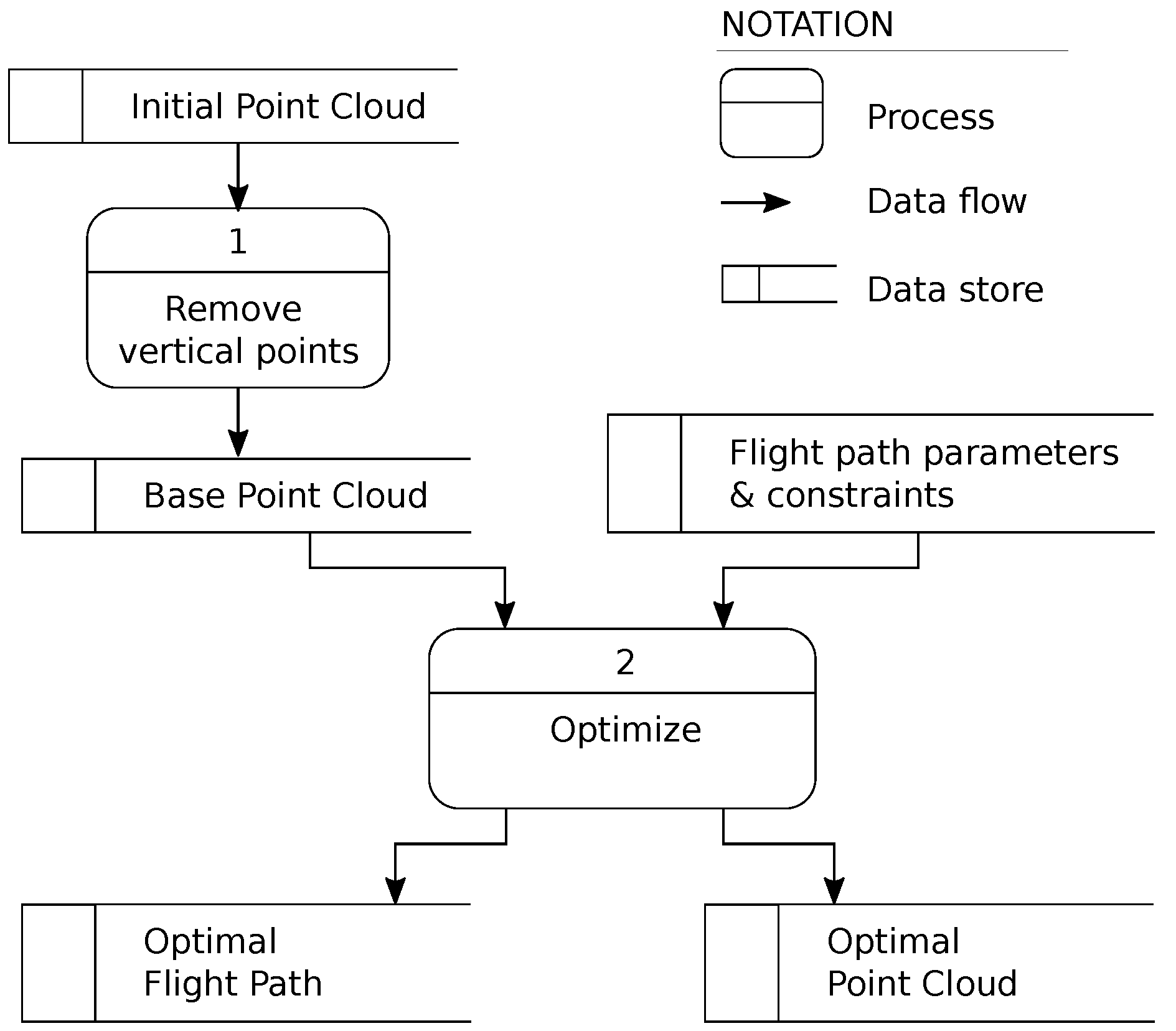
An overview of the data flow and processes employed in the research are presented in Figure 2. In addition to the flight path parameters and constraints, the optimization (Process 2 in Figure 2) requires some knowledge of the target urban environment including at least a rough representation of the street topography and building geometries. In this research, the urban environment is represented as a special kind of point cloud, called a base point cloud. A base point cloud represents the data captured in a manner that is likely to be sub-optimal for vertical surface documentation. To avoid introducing bias into the baseline data through the existence of some vertical data, the proposed approach advocates its wholesale removal. A base point cloud can be obtained by removing points on vertical surfaces from a pre-existing point cloud of the area of interest (Process 1 in Figure 2). Where a pre-existing point cloud is unavailable, a base point cloud can be generated by rasterizing any 3D model of the city [43]. The optimization described in the remainder of this section aims to search for the most optimal flight path in the form of one that yields the largest number of vertical points. The point cloud derived from the optimal flight path is referred to as the optimal point cloud.

3.1. A Genetic Algorithm for LiDAR Flight Path Optimization

The genetic algorithm was devised to maximize vertical surface point generation. Algorithm 1 presents the pseudo-code of a typical GA. Given an initial set of randomly generated flight grids ($G_{\mathrm{initial}}$), new generations of flight grids are iteratively created by biologically inspired processes, including selection, mutation, and crossover. The selection is based on a fitness function that provides a metric to evaluate the quality of an individual (i.e., flight grid) [lines 2 & 8 in Algorithm 1]. In the context of urban LiDAR flight path optimization, the fitness function evaluates a flight grid based on the quantity of vertical points the flight grid generates (further explained in Section 3.2).

Based on the fitness scores (i.e., outputs of the fitness function), two subsets are selected from an original generation ($G_i$) using operations Select_S and Select_O on lines 4 and 5. The first subset (called survivors, $S_i$) derived from function Select_S contains high-performing individuals that are passed unchanged onto the next population (line 4 in Algorithm 1). The second subset derived from function Select_O contains other high-performing individuals that are combined pairwise via a process called crossover to create offspring, $O_i$ (line 5 in  Algorithm 1). The offspring are supposed to inherit good characteristics from the high-performing individuals in the previous population. Subsequently, a small fraction of the offspring, $O_i$, is randomly mutated (line 6 in  Algorithm 1). The mutation process is supposed to create random characteristics absent in the previous population. The survivors, $S_i$, and the offspring, $O_i$, are combined to form the next population, $G_{i+1}$ (line 6 of Algorithm 1). New generations of flight grids are iteratively generated, until the results converge. Namely, the fitness scores are not further improved after (1) a certain number of iterations is reached, (2) the best fitness score exceeds a certain value, or (3) the number of iterations reaches a predefined value. The GA returns the best individual of all flight paths generated.

Algorithm 1 Typical structure of a genetic algorithm

There are many GA implementations that differ slightly. In this research, Jenetics, a Java GA library by Wilhelmstötter [44] was used. Jenetics provides base, domain classes (e.g., Population, Phenotype, Chromosome, and Gene), operation classes (e.g., Alterer and Selector), and Engine classes to connect all components into a GA. A Population is a set of Phenotypes, each of which is a Genotype (i.e., genetic constitution of an individual) with a fitness score. A Genotype is composed of multiple Chromosomes. Each chromosome consists of a set of Genes. A key step in the application of GA to LiDAR flight path optimization is to translate the problem domain into GA concepts.

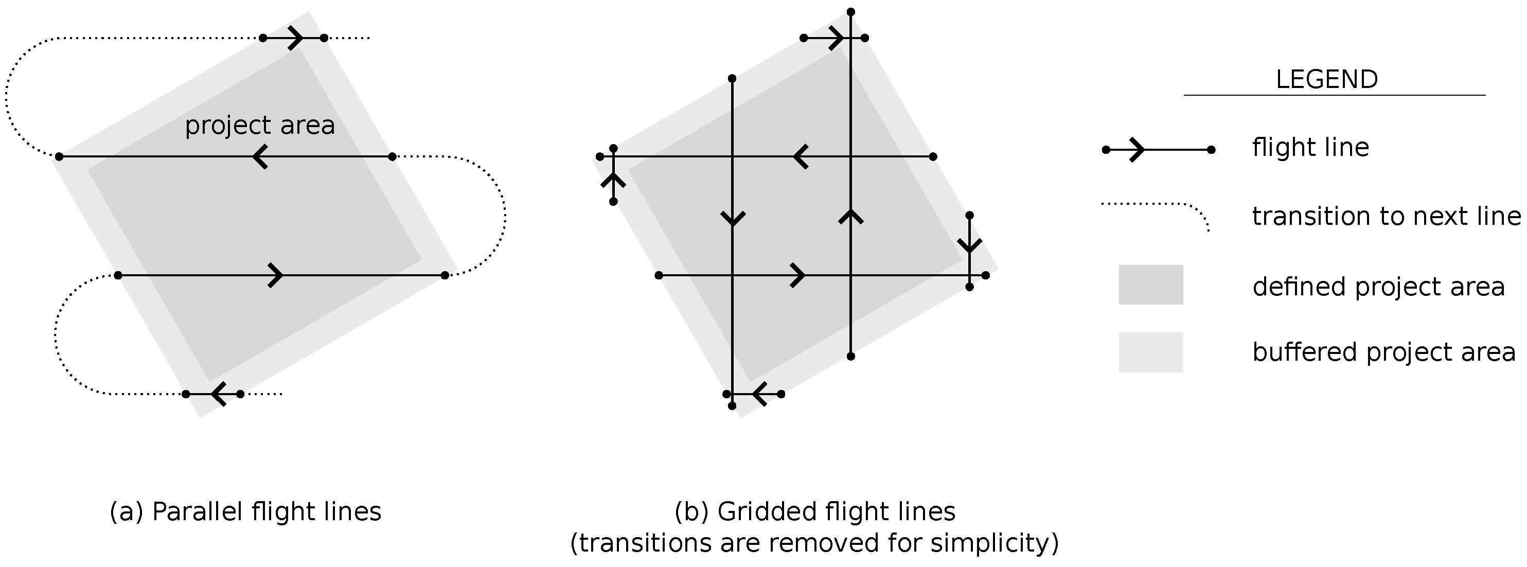
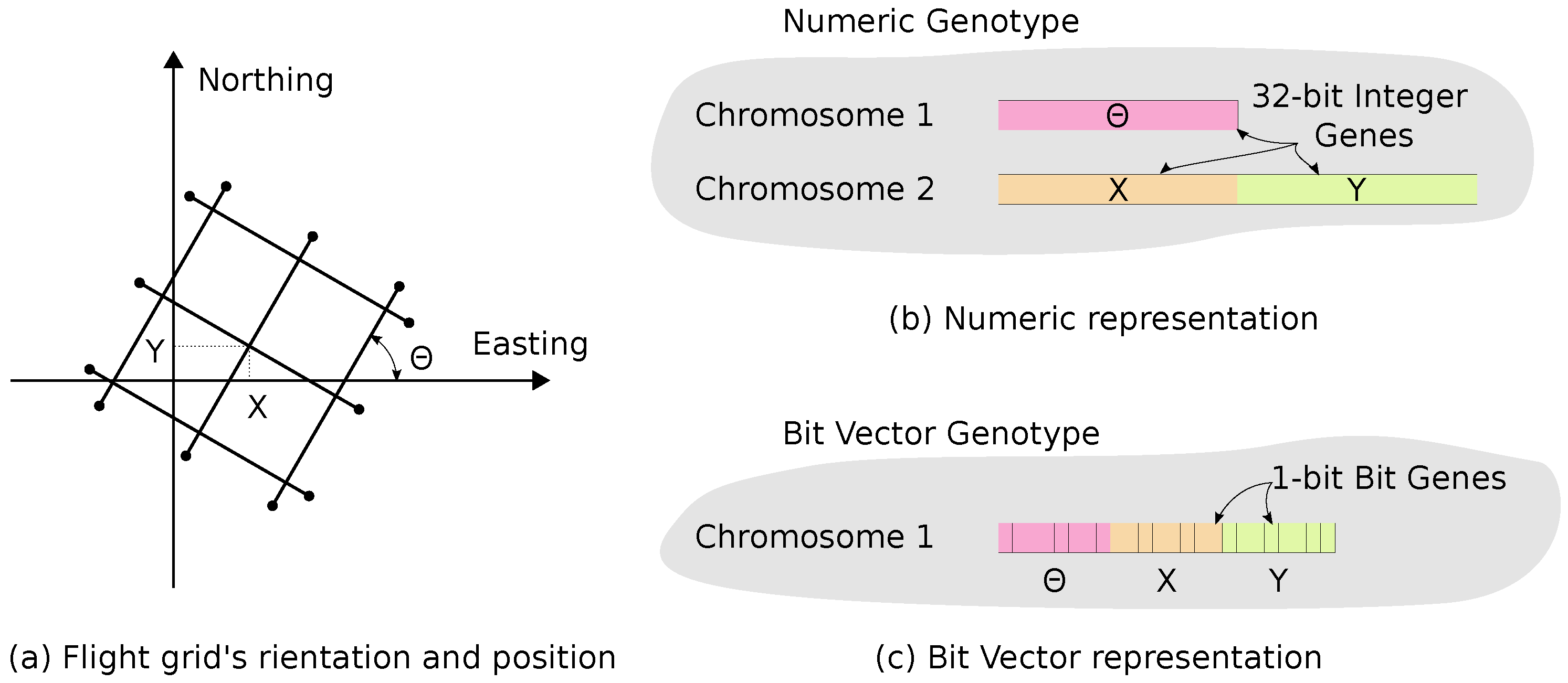
Building upon the work of Hinks et al. [23], a flight grid pattern (Figure 1b) is defined. A flight grid is represented by three numeric parameters $(\mathrm{\Theta },X,Y)$ that define the orientation and position of the flight grid (Figure 3a). All three parameters are bounded, $\mathrm{\Theta }\in [0,90)$, $X\in [-s/2,s/2)$, $Y\in [-s/2,s/2)$; where s is the flight line spacing (Figure 3a). Two different GA representations of flight grids are considered. The first representation (called Numeric) is based on the Integer Chromosome built-in Jenetics. A Genotype (i.e., a flight grid) is composed of two Integer Chromosome (Figure 3b). The first Chromosome consists of a single (32-bit) Integer Gene that represents $\mathrm{\Theta }$. The second Chromosome is comprised of two (32-bit) Integer Genes that represent X and Y. In the second representation (called Bit Vector), each value of $\mathrm{\Theta }$, X, and Y is encoded as a binary string (8-bit integer) and represented as a BitVector Chromosome. A Genotype in this second representation contains only a single Bit Vector Chromosome, which is composed of 32 Bit Genes (Figure 3c). While a Numeric representation is more straightforward, it appears to be less effective, based on some preliminary testing by the authors. Specifically, the BitVector representation allows faster convergence.

In addition to the representations described in this section, the GA implementation requires a definition of a fitness function, which is explained in Section 3.2. Apart from these, all other elements of the GA algorithm (e.g., operation classes and evolution engine) were adopted directly from Jenetics.

3.2. A Beam Tracing Algorithm to Simulate Vertical Points Captured by a LiDAR Flight Path

Given that a significant sidelap (>67%) is allowed between every pair of adjacent flight swaths (i.e., stripes of point data captured by a flight line), sufficient capture of the geometry of horizontal surfaces such as ground and building roofs is trivial [20]. Instead, the main challenge is to capture vertical surfaces such as building façades [23]. As such, the number of points on vertical surfaces that a flight grid generates is a straightforward indicator by which measure how good or bad a flight grid is, in terms of documenting an urban area. This is used as the basis of the fitness score. While the output is simple to understand, computing it is complex, as the simulation requires knowledge of the flight geometry (i.e., altitude, position and orientation of the flight grid), the urban geometry (i.e., buildings and other urban objects), and certain scanner settings (e.g., scan angle, angular resolution). Figure 4 illustrates the spatial model underlying the estimation of the number of vertical points that a flight grid can generate (i.e., the fitness score). The flight geometry is in all cases assumed to be composed of a set of straight flight lines separated by a predetermined, uniform flight line spacing, $s_l$. Each flight line is discretized into a set of way points, spaced $s_w$ apart (Figure 4a). By discretizing the flight lines, the real, continuous movement of the aircraft is modeled as a discrete stepwise traverse across the way points. As previously noted, the urban geometry is represented using a base point cloud, which eliminates the need to model the complex urban environment manually or via a simplified mathematical model, which avoids any inaccuracies that could be introduced through such approaches. A scanner’s settings are usually available in equipment specification sheets and can be input directly into the simulation. Given the spatial model (Figure 4), which encapsulates the flight geometry, urban geometry, and scanner settings, laser beams can be simulated from every way point toward the portion of the base point cloud that intersects the field of view (FOV) corresponding to each way point (Figure 4c). Because the base point cloud only consists of non-vertical points, if a laser beam arrives in the vicinity a point in the base point cloud (beams $b_1$−$b_2$ and $b_4$−$b_{11}$ in Figure 4c), the laser beam is assumed to be incident on a non-vertical surface. If a laser beam does not approach any point in the base point cloud (e.g., beam $b_3$ in Figure 4c), then further computation (detailed in the remainder of this section) is performed to confirm whether the beam strikes a vertical surface.

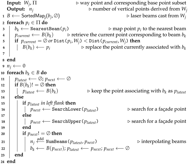
Figure 4c presents a subset $\mathrm{\Pi }$ of the base point cloud P within the FOV of a way point, $W_j$, and the laser beams B cast from this way point. The beam tracing from each way point is performed in the 2D vertical plane containing the way point using Algorithm 2. The laser beams are sorted counter-clockwise based on the beams’ angles to nadir ($b_1$ to $b_{11}$ in Figure 4c, Algorithm 2 line 1). Each point in subset $\mathrm{\Pi }$ is mapped to its nearest laser beam (Algorithm 2, line 3). If multiple points are mapped to the same beam (e.g., $p_1$, $p_2$ and $p_3$ are mapped to $b_1$ in  Figure 4b), the point closest to the way point is kept (e.g., $b_3$). All further points are discarded, as the first point is assumed to obstruct all laser energy. The discarded points are colored in grey in Figure 4c. The logic is represented on lines 4–6 in Algorithm 2.

In the next step (lines 10–23 in Algorithm 2), the laser beams and their corresponding base points are evaluated in their sorting order (i.e., $b_1$ to $b_{11}$, beam set B on line 10 in Algorithm 2). During the evaluation, when a non-empty beam (i.e., a beam that associates to a base point) is encountered (Algorithm 2 line 12), its corresponding base point is recorded (i.e., $p_{latest}$). As  previously mentioned, such a beam is assumed to be incident on a non-vertical surface. When the encountered beam is empty (i.e., the beam does not associate with any base point, Algorithm 2 line 14), the algorithm traces back to the latest recorded base point, $p_{latest}$. In the example in Figure 4c, the first empty beam is $b_3$, and the latest recorded point is $p_4$. The algorithm searches the neighborhood of $p_{latest}$ for structures that resemble building façades (Figure 4d). The search domain differs depending on the relative position of $p_{latest}$, with respect to nadir. If $p_{latest}$ is in the left flank of the FOV (Algorithm 2 line 15), then the algorithm searches the lower part of the neighborhood of $p_{latest}$ (Algorithm 2 line 16). Otherwise, the upper part of the neighborhood is searched (Algorithm 2 line 18). If the search returns another point ($p_{next}$), which together with $p_{latest}$ forms a vertical structure, the number of laser beams striking on the vertical segment $(p_{latest},p_{next})$ is interpolated (line 21 in Algorithm 2). The total number of such vertical laser beams is the output of the beam casting from $W_j$ is calculated (Algorithm 2 line 21). The fitness score of a flight grid is the total number of such beams derived from all way points of the flight grid. Notably, the number of beams is assumed to be equal to the number of points yielded by a flight grid since a beam striking on a façade surface usually results in a single point return. The beam tracing algorithm accounts for both self-shadow and street-shadow based occlusions as defined by Hinks et al. [23]. The use of a base point cloud is designed explicitly to allow a more accurate representation of the complex urban environment and, thus, a more robust measure of the algorithm’s output. The beam casting algorithm in Algorithm 2 and its use in computing the fitness scores for the optimization clearly reflect the objective of the optimization.

Algorithm 2 Beam casting from a specific way point

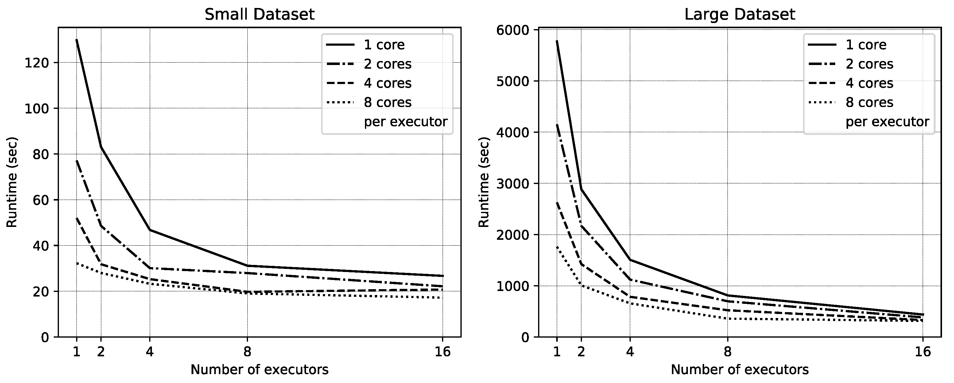
3.3. A Distributed Computing Strategy for Fitness Function Evaluation

The beam tracing introduced in Section 3.2 is not particularly computationally complex, nor does it involve big data. In contrast, the actual computational challenge is in the fitness computation, which comes from two sources. First is that the number of way points can be large. Thus, the beam tracing must be performed thousands or millions of times. Second, the selection of base points inside the FOV of a way point is an expensive process. Matching base points to their corresponding way points is essentially a spatial join between two potentially large datasets, $P\bowtie W$. The point dataset, P, can contain millions or even billions of points depending on the spatial extent and the point density. The number of way points in W can be several thousands or more depending on the flight geometry and the discretization resolution. A base point $p_i\in P$ is joined with way point $w_j\in W$, if the FOV of a $w_j$ contains $p_i$. The join is many-to-many, where a way point is joined with multiple base points, and a base point is joined with multiple way points. Algorithm 3 presents a complete strategy for the fitness score computation that addresses both challenges.

Algorithm 3 Parallel algorithm for computing the fitness score (i.e., the total number of laser beams incident on vertical surfaces) of a flight grid

Algorithm 3 computes the fitness score, n, of a candidate flight grid using the base point cloud, P, and the flight parameters, $F(X,Y,\mathrm{\Theta })$. The algorithm is composed of two stages. Stage 1 (the for loop on lines 2–5 in Algorithm 3) performs $P\bowtie W$ (i.e., base points and way points joint). Stage 2 (the for loop on lines 9–11 in Algorithm 3) performs beam casting for each way point as described in Section 3.2. Between the two stages is the data shuffling operation (i.e., AggregateByKey, line 8 in Algorithm 3), which aggregates base points by their corresponding way points. Both for loops are straightforwardly parallelizable. Each execution of the first for loop takes an individual base point $p_i$, calculates coordinates of the way points $W_j$ corresponding to the given base point and add the way point – base point pairs to $Se{t}_{ij}\left([W_j,p_i]\right)$. The calculation of way point coordinates starts with transforming the coordinate system (lines 3 in Algorithm 3) so that the flight lines are parallel to the coordinate axes.

$$\begin{array}{cc}\hfill lIdx& =\left[\frac{x_i}{s_l}\right]\hfill \end{array}$$

(1a)

$$\begin{array}{cc}\hfill wIdx& =\left[\frac{y_i}{s_w}\right]\hfill \end{array}$$

(1b)

$$\begin{array}{cc}\hfill {\mathsf{\Omega }}_{swath}& =Htan\left({\phi }_{max}\right)\hfill \end{array}$$

(1c)

Consider a set of flight lines parallel to the Y axis as in Figure 5, the algorithm calculates the index of the flight line closest to $p_i$ using Equation (1a). The squared brackets denote rounding to the nearest integer. In the example in Figure 5, the closest flight line to $p_i(x_i=137.2,y_i=0.7)$ is $l_2$ because $lIdx=[x_i/s_l]=[137.2/80.0]=\left[1.715\right]=2$. On the given flight line, the way point closest to $p_i$ is calculated using Equation (1b). In Figure 5, $wIdx=[y_i/s_w]=[0.7/0.5]=\left[1.4\right]=1$. Hence, $p_i$ is closest to way point $w_1$ on flight line $l_2$. In addition to the closest way point, $p_i$ is mapped to way points on other flight lines nearby the closest flight line, as long as the Euclidean distance from $p_i$ to the line calculated in the XY plane is shorter than the expected half swath width. The half swath width (${\mathsf{\Omega }}_{swath}$) is calculated as in Equation (1c) and is constant for the entire flight mission. Function WayPoint on line 4 of Algorithm 2 encapsulates the way point calculation expressed in Equation (1a–1c). Thanks to the coordinate transformation, the spatial mapping of base points to way points becomes the simple arithmetic formulae in Equation (1). More importantly, both of the transformations (i.e., CoordTransform and WayPoint) are performed independently for each base point. As $Se{t}_{ij}\left([W_j,p_i]\right)$ is a distributed dataset, adding the newly computed way point — base point pairs do not require any synchronization among elements of the dataset. Every step in the first for loop is parallel. In the second for loop (lines 9–11 of Algorithm 3), each execution takes an individual way point, $W_j$, and the corresponding base point subset $\mathrm{\Pi }$ to perform the beam casting algorithm described in Algorithm 2 and Section 3.2. Similar to the first for loop, the second for loop is straightforwardly parallelizable since each individual execution is independent.

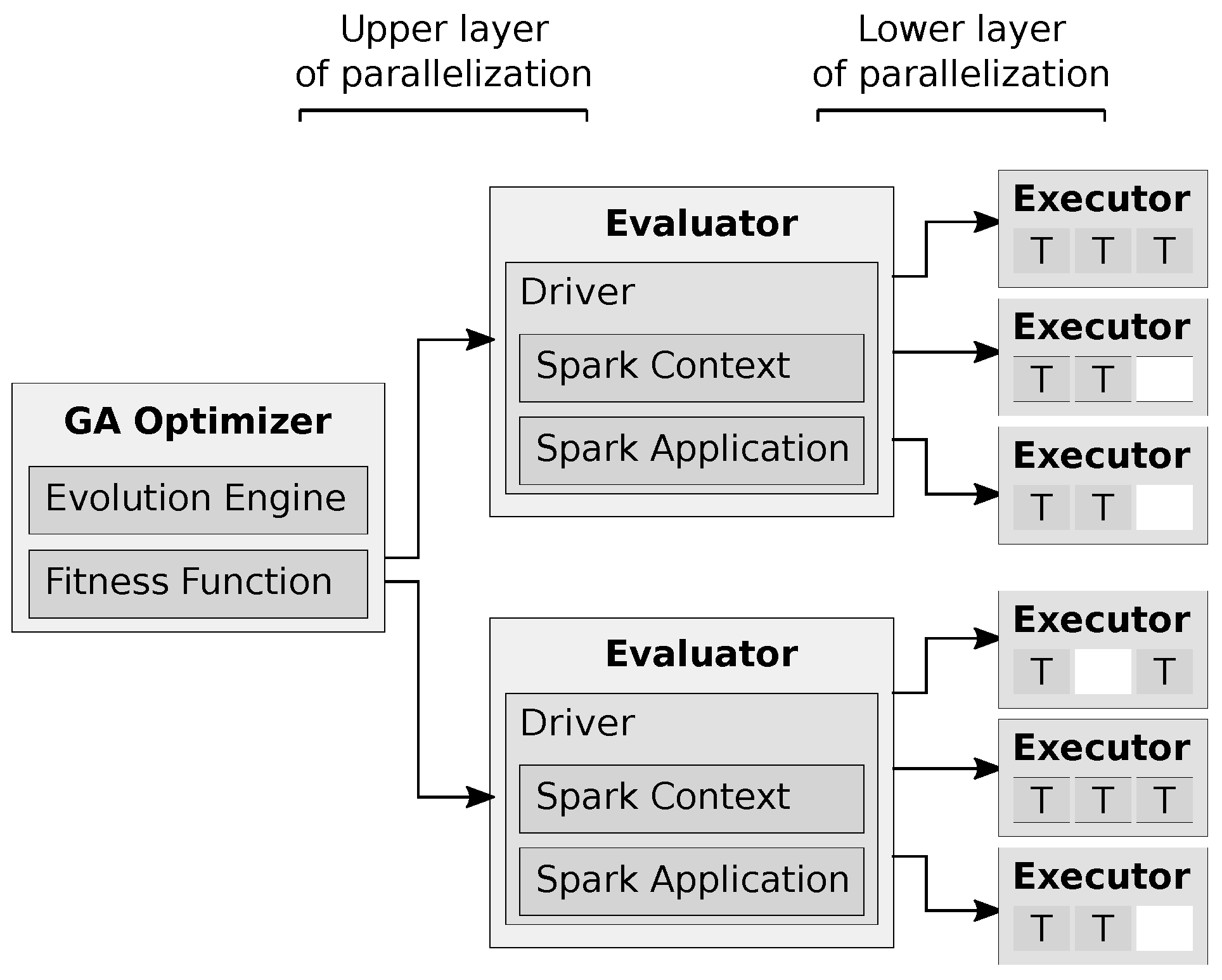
Figure 6 shows the data lineage corresponding to Algorithm 3. All datasets in Algorithm 3 are distributed datasets, called Resilient Distributed Datasets (RDD) in Spark, the distributed computing framework selected to implement the algorithm. Each dataset (e.g., the base point cloud, P) is divided into multiple partitions distributed across multiple executors for parallel transformation and computation. Executors are distributed software processes that can reside on different nodes of a computing cluster. In Figure 6, each rounded box represents a data partition, and each stack of partitions represents an RDD.

Notably, the transformations within Stage 1 and Stage 2 do not require data to be exchanged between partitions, and their data flows are confined to be within the partition boundaries. Thus, no communication between executors or nodes is needed. The CoordTransform and WayPoint transformations in Stage 1 are applied for each base point $p_i$. Similarly, the BeamCasting transformation in Stage 2 is applied on each way point and a limited subset of base points ($\mathrm{\Pi }$) corresponding to the way point. All of those transformations are easily parallelizable, because manipulation of one record is totally independent of other manipulations and side effects. In addition, the amount of data involved in each transformation is limited. Thus, each transformation is performed in memory.

The operation that is not straightforwardly parallelizable is the aggregation of base points by way point that occurs between the two stages. That operation requires physical movement of data between partitions that potentially reside on different nodes. Multiple partitions need to be combined to build partitions for a new RDD. The complex operation is implemented based on the parallel AggregateByKey function in Spark. The AggregateByKey function aggregates data within each partition before shuffling the data between nodes, thereby minimizing data transfer across the cluster. Another operation that needs data transfer across nodes is the final function that gathers the numbers of vertical points from all partitions and computes the final sum. That operation is straightforward and is implemented using the Collect function in Spark.

In summary, the principal strategy behind the fitness score computation is data parallelism. The algorithm is composed of two map transformations and one data shuffling transformation. The datasets are divided into small partitions distributed across multiple executors. During each map transformation, multiple executors work in parallel to apply the same transformation to their data partitions. The data partitions are kept sufficiently small so that every transformation can be performed within the memory space allocated to each executor. The shuffling transformation that occurs between the two map transformations is the most complex part of the algorithm. That shuffling transformation is implemented based on a highly optimized function in Spark (i.e., AggregateByKey). Throughout that algorithm, the computation is decomposed into loosely coupled transformations that are conducted by different executors in a highly independent manner. Expensive communication across executors and nodes is restricted. As such, the algorithm is suitable for being deployed on a distributed-memory cluster in which the computing nodes that host executors do not share a memory space and use an interconnect for their limited communication.

3.4. Multiple Evaluators—An Additional Level of Parallelism

Section 3.2 and Section 3.3 describe the parallel computing strategy that enables the evaluation of one flight grid. That parallelization is herein referred to as the lower layer of parallelization. Atop that, an upper layer of parallelization is introduced by allowing multiple evaluators to simultaneously evaluate the fitness scores of different flight grids. The two layers of parallelization are depicted in Figure 7. The GA optimizer at the upper layer controls the entire optimization process. The GA optimizer is a multi-threading Java process that has one thread performing the GA operations and multiple threads connecting to different parallel evaluators. The setup is aimed for deployment on a distributed environment in which the GA optimizer and the evaluators reside on independent computing nodes that do not share disk or memory spaces. The GA optimizer and the evaluators exchange limited data via socket connections. Such a distributed architecture easily allows scaling the computing resource (e.g., adding more parallel executors) to accommodate increases in the workload (e.g., an increase in input dataset). On the lower layer, each Evaluator is an independent Spark application, which sequentially analyzes its subset of flight grids using multiple, parallel executors of a distributed memory cluster as described in Section 3.3. In addition, each executor can perform multiple, parallel tasks (denoted as T in Figure 7) using multi-threading. The multiple, parallel levels allow an efficient usage of available computing resource to perform the computation rapidly. Compared to the lower layer of parallelization explained in Section 3.2 and Section 3.3, the upper layer of parallelism is more straightforward, because the evaluation of one flight grid is wholly independent of the other flight grids. What could partially impede the parallelism on this layer is the evaluator coordination performed by the GA Optimizer (e.g., assigning flight grids; gathering and synchronizing results). While the upper layer of parallelization can accelerate the optimization more straightforwardly, it does not target the big data challenges addressed by the lower layer. Thus, a combination of the two levels is needed.

4. Results

This section presents the computational experiments that demonstrate the success of the GA optimization strategy and evaluate the computational performance and scalability of the parallel algorithms presented in Section 3. In addition, the accuracy of the proposed method was evaluated based on two actual test flights. The two test flights followed flight grids that were selected based on their prediction of achieving the best and worst outcomes as a function of their having the highest and lowest fitness scores identified by the GA, respectively. The flights were conducted at 300 m above the ground level at a speed of 50 knots. The flight line spacing ($s_l$) was 80 m, which is equivalent to a side lap of 77%. The flights were conducted with a Riegl Q680i scanner with a pulse rate of 400 kHz and an FOV of 60${}^{\circ }$. Those flight and scanner configurations were set as fixed parameters in the GA optimization and the test flights.

A study area of 1km${}^2$ in Sunset Park, New York (Figure 8) was selected based on local flight permissions. The main input of the optimization process was the base point cloud of the area. For this, a publicly available, city-wide LiDAR scan of New York City from 2017 [5] was used. Those data were acquired at 1800 m above the ground level with parallel a flight line pattern (e.g., Figure 1a) and an average sidelap of 60% [3]. The aggregate point density calculated on horizontal surfaces was 11 points/m${}^2$. The total number of base points after vertical point removal was 9,688,794. All computational experiments were performed using a distributed-memory computer cluster of 18 nodes connected with 100 Gb/s Ethernet connection. Each node had 2 × 24 core Intel Xeon [email protected] and 384 GB memory. Strictly speaking, the cluster is hybrid, as it had multiple distributed-memory nodes, each of which had multiple shared-memory cores. The cluster is a shared facility that simultaneously accommodates many other computations apart from the experiments reported in the section.

4.1. GA Optimization Results

To confirm the success of the GA in LiDAR flight path optimization, the GA was executed with two opposing objectives: maximizing and minimizing the fitness function. There were 36 flight grids per generation. The crossover and mutation rates were 0.8 and 0.05, respectively. Two flight grids were selected from each generation as survivors. As in any stochastic solver, there is no way to know a priori which parameters are optimal for a new problem space. The initially selected parameters were set based on practical experience and trial and error. Regarding the specific number of survivors, if less than one survivor is kept, a convergence may be harder to achieve as elite candidates are lost during the evolution process. If too many survivors (e.g., 50% of the population) are kept, the optimization may not be able to explore the search space and may easily become caught in local maxima.

The evolution processes corresponding to the two opposite objectives are presented in Figure 9a. Each rotated bell curve represents the fitness score distribution of a generation. The blue curves represent the GA progress when the objective was maximization. The orange curves correspond to the minimization. As evident from Figure 9a, the GA operators successfully drove the fitness scores towards the defined objectives. The blue curves progressed upwards, while the orange curves progressed downwards. While Figure 9a shows all 32 generations tested, the results converged from the 10th generation for both the maxi- and minimization. The executions resulted in the most and the least optimal flight grids, as shown in Figure 9b,c, respectively. The difference in vertical point yield between the most and least optimal flight grids was projected to be approximately 13%. The most optimal flight grid was nearly diagonal to the main street axes (Figure 9b) versus the least optimal flight grid, which was nearly orthogonal (Figure 9c). This result agreed with the previous finding by Hinks et al. [23] even though Hinks et al. [23] arrived at that conclusion via simplistic geometric modeling. The agreement of the two approaches is attributable to the dominant rectilinear layout of the street axes in the study areas. In the remainder of the paper, the most optimal flight grid is referred to as the Diagonal flight grid and the least optimal as the Orthogonal flight grid.

To understand the actual effectiveness of the Diagonal and Orthogonal flight grids identified by the GA in capturing vertical surface structures, the two flight grids were flown on 11 May 2019, as part of a single mission. The point clouds derived from the two flights are herein referred to as the Diagonal and Orthogonal point clouds. The point density histograms of the two point clouds are shown in Figure 10. The point density was calculated using the local point density index [45], which took into account the local surface orientation.

Compared to the Orthogonal point cloud, the Diagonal point cloud had more points on vertical surfaces (indicated as V in Figure 10). With respect to the point density on horizontal surfaces, the Diagonal point cloud had more higher-density points (270 points/m${}^2$) and fewer lower-density points (250 points/m${}^2$) [indicated as H in Figure 10]. To quantify the actual difference, the number of vertical points in the two point clouds were counted. A point was considered vertical if its local fitting surface was within 10${}^{\circ }$ from a perfectly vertical plane. According to that analysis, the Diagonal point cloud had 16% more vertical points compared to the Orthogonal point cloud. That level of difference was slightly higher than the 13% predicted by the proposed algorithm (Figure 9a). Given that the study area is populated with mostly low-rise to medium-rise buildings, the 16% gain in vertical points is significant. If the study was conducted in a metropolitan area with taller buildings and narrower alleyways, the higher effectiveness of the Diagonal flight grid would be even more notable.

Figure 11 and Figure 12 provide a more detailed analysis of the vertical point densities of the Diagonal and Horizontal point clouds. Figure 11 shows the point distribution on two building façades A and B, which both faced a narrow alleyway. Such façades are susceptible to street occlusion and are typically missed by high-altitude ALS flights. Façade A is particularly challenging, because the space between the roof edges over the alleyway, where laser beams could enter to capture the façade, was only 1.3 m wide. Nevertheless, both façades were captured with reasonable densities and completeness in the Diagonal flight grid, as well as a significantly higher density than in the Orthogonal, as observable in both the visualization and histograms. Compared to the Orthogonal flight grid, the Diagonal flight grid captured 24% and 61% more vertical points on façades A and B, respectively. This translated to a significant difference in average vertical point density.

Shown in Figure 12 are the North-East and South-West façades of the Brooklyn Army Terminal (BAT), a standalone building with no tall structures nearby. So, unlike façades A and B in Figure 11, the BAT façades were not susceptible to street occlusion. For these façades, the advantage of the Diagonal flight was less dramatic. While the Diagonal flight grid captured 18% more vertical points on the North-East façade (see point density histogram), the density distribution was less uniform, as the façade was at the edge of a Diagonal flight grid flight line. In fact, on the South-West façade, the Diagonal flight grid captured 7% less vertical points.

While not every façade was better captured by the Diagonal flight grid, the overall higher effectiveness of the Diagonal flight grid compared to the Orthogonal flight grid was observed in both the overall statistics of the complete datasets and from most specific detailed observations. The Diagonal flight grid captured 16% more vertical points than the Orthogonal flight grid. That 16% difference was slightly higher than the 13% predicted by the algorithms presented in Section 3. Nevertheless, the results satisfactorily substantiated the accuracy of the proposed methodology. The remainder of the section analyzes the computational efficiency of the proposed algorithms.

4.2. Performance Evaluation

The GA executions shown in Figure 9 took 99 and 65 min for maximizing and minimizing the objective functions, respectively. In each execution, four evaluators were used. Each evaluator had four executors with four cores. The numbers of evaluators, executors, and cores were selected based on the computational experiments presented later in this subsection. The total runtime of less than 2 h makes the proposed method practical and feasible for an actual flight planning. Given the two layers of parallelization, more computing resource can be flexibly added to speed up the optimization as needed. In the following subsections, the efficiency of the two layers of parallelization is analyzed in detail.

4.2.1. Lower Layer of Parallelization

To evaluate the efficiency of the lower layer of parallelization, different numbers of executors and cores were used to compute the fitness score of a fixed flight grid. The runtimes of the fitness score computations are presented in Figure 13 (Small Dataset) and

Table 1. Efficiency of the lower level of parallelization—Small Dataset.

			Num. Executors
			1	2	4	8	16
num. cores per executor	1	Runtime (s)	130	83	47	31	27
		Speedup	—	1.6	2.8	4.2	4.9
	2	Runtime (s)	77	49	30	28	22
		Speedup	1.7	2.7	4.3	4.6	5.8
	4	Runtime (s)	52	32	25	20	21
		Speedup	2.5	4.1	5.1	6.6	6.2
	8	Runtime (s)	32	28	23	19	17
		Speedup	4.0	4.6	5.6	6.8	7.5

. The reported runtimes captured the entire process from the time each Spark job was submitted until it terminated. In addition to the net computing time, all overheads such as the time required for the cluster management system to allocate resources, release resources, and clean up temporary data were included. In general, the runtime reduced when more executors and cores were added. The speedup factors in Table 1 measure the reduction in runtime when more resources are used. The speedup factors were calculated as $S=T_{serial}/T_{e,c}$, where $T_{serial}$ is the serial runtime (1 executor, 1 core) and $T_{e,c}$ is the runtime corresponding to a parallel execution that uses e executors and n cores. The speedup factors in Table 1 were low. In particular, the runtime reduced only 4.9 times when the number of executors increased by 16 times (given one core per executor). In an ideal scenario, an increase of resource by n times should result in n times reduction in runtime. While such an ideal speedup is rarely achievable in practice [13], the factor of 4.9/16 is low. The low efficiency is attributable to the small size of the input base point cloud (i.e., under 10 million points). The net computing time for the small dataset was in the range of under 40 s when multiple executors and cores were used. That computing time was comparable to the overheads. While parallelism did reduce the net computing time, it did not affect the overheads. Thus, the efficiency of the parallel solution was hidden when the test dataset was small.

To confirm the actual efficiency of the proposed parallel algorithm for flight grid evaluation, an experiment was conducted for an additional area 46 times larger than the study area (see Appendix A). The large study area shown in Figure A1 is located in Brooklyn, New York and encloses the Sunset Park site shown in Figure 8. The number of base points was over 460 million points. The runtimes for the large experiment are reported in Figure 13 (Large Dataset) and

Table 2. Efficiency of the lower level of parallelization—Large Dataset.

			Num. Executors
			1	2	4	8	16
num. cores per executor	1	Runtime (s)	5771	2884	1507	812	439
		Speedup	—	2.0	3.8	7.1	13.1
	2	Runtime (s)	4151	2171	1121	697	383
		Speedup	1.4	2.7	5.1	8.3	15.1
	4	Runtime (s)	2627	1423	785	522	331
		Speedup	2.2	4.1	7.4	11.0	17.4
	8	Runtime (s)	1762	1008	657	359	315
		Speedup	3.3	5.7	8.8	16.1	18.3

. The overheads were insignificant relative to the net computing time. Thus the efficiency of the parallel algorithms appeared much more clearly. A speedup factor of 13.1 was achieved when increasing the number of executors from 1 to 16 (given one core per executor). Adding more executors resulted in a higher level of efficiency compared to adding cores. For example, the speedup was 7.1 when increasing the number of executors by 8 times, while the speedup was only 3.3 when octupling the number of cores. Among all tests conducted, the highest speedup factor was 18.3 when 16 executors and 8 cores per executor were used. The result successfully demonstrated the efficiency of the lower layer of parallelization.

4.2.2. Upper Layer of Parallelization

Similar to the lower layer, the upper layer of parallelization was evaluated by varying the number of evaluators and observing the runtime. To avoid the randomness of the GA process, the experiments were conducted for a fixed generation of 36 flight grids. Each evaluator was given four executors and each had four cores. Figure 14 and

Table 3. Efficiency of the upper level of parallelization.

	Num. Evaluators
	1	2	3	4
Runtime (s)	454	282	186	144
Speedup	—	1.6	2.4	3.2

show the results of the experiments. The runtime reduced when more evaluators were added. The speedup factors were 1.6, 2.4, and 3.2 when the number of evaluators increased by 2, 3, and 4 times, respectively. In the current implementation, while the number of flight grids was distributed evenly among evaluators, there was occasionally an observable imbalance in response time between evaluators. At the end of each GA generation, all faster evaluators had to wait for the slowest evaluator, before the GA operators could generate the next generation. A significant imbalance in response time between evaluators could impede the efficiency of the upper layer of parallelization. Such imbalance could be alleviated by a more sophisticated load balancer, which may allocate tasks based on the actual response of the evaluators to minimize wait time. Nevertheless, having this upper level provides additional control of the total level of parallelism. In the particular case of the small dataset experiment, adding three more evaluators (each with four executors) was more efficient than adding the same number of executors directly to the one existing evaluator. With the same amount of computing resource (i.e., 16 executors × 4 cores), the former approach resulted in a reduction of 1.2 times in runtime (Table 1), while the latter approach resulted in a reduction of 3.2 times (Table 3). The combination of both levels of parallelization resulted in a maximum overall efficiency factor of 32.5/64. In particular, the evaluation of one grid without parallelism (i.e., one evaluator, one executor, and one core) took 130 s (Table 1), whereas the evaluation of 32 grids with four evaluators, four executors, and four cores took 144 s (Table 3). The speedup factor is calculated as $130/\frac{144}{32}$ = 32.5, while the total number of parallel cores is $4\times 4\times 4=64$.

5. Discussion

This paper introduces a novel, scalable, and computationally efficient method to optimize LiDAR flight path planning for specific objectives within a dense urban environment. The proposed method employs a genetic algorithm, a dual parallel computing framework, and low-density, publicly accessible data sets. This enabled optimization to be objectively based on real-world characteristics of individual geo-locations. This was demonstrated herein for maximizing vertical point density acquisition, in which a 16% increase in vertical point yield was obtained even in a region dominated by low-rise structures and relatively wide streets, which meant that there was a relatively sparsity of vertical façade areas to be documented compared to a central business district and that there was a low level of street shadowing since the street widths provided significant separation in that direction. Thus, as expected in such a region, the selected cases showed that achieving reasonable vertical coverage for unoccluded, standalone structures could be possible with little consideration to flight path orientation (Figure 12). However, even under these relatively undemanding conditions, when structures (even relatively low-rise ones) were closely spaced, achieving full coverage was problematic (especially on the lowest stories) without a directed data acquisition scheme (Figure 11). As such, in high-density areas, with narrower streets or a more mixed condition of building heights and street widths, some form of the diagonal grid would be expected to produce even more dramatic results.

While the Sunset Park case furnished a quantifiable demonstration of the potential benefits of the optimization, the exercise highlighted several more fundamental contributions. The first is the incorporation of a multi-objective framework with a low-density base point cloud. While the current optimization included only a handful of variables and imposed extremely limited ranges on them because of aviation authority flight restrictions and the imposition of a set of parallel lines to be followed by a manned aircraft, this is not necessarily reflective of the future aerial LiDAR. The past decade has shown rapidly growing capacities and commercial options of unmanned autonomous vehicles as individual units and swarms (e.g., [46,47,48]). The proposed framework could be further developed for planning complex flight paths that may be composed of curved and/or non-parallel flight lines as often seen in UAV mapping. A different algorithm could be substituted for the beam tracing algorithm in the framework to model data collected by complex sensor systems which may include multiple, independent sensors of different types (e.g., LiDAR and hyperspectral).

The GA was demonstrated in this research as being effective in searching for optimal flight grids based on their ability to capture vertical surfaces. However, that specific application does not reflect the capability of the proposed computing framework. Since GAs are known for their ability to incorporate multiple optimization objectives, the main computing framework can be amended and connect to different flight path evaluators to optimize for multiple objectives. The use of a base point cloud that is generated from a publicly accessible, sparse point cloud captured by typical, high-altitude ALS missions as the primary geometric input for the optimization allows for a more realistic representation of the actual, complex, urban configuration, which contributes to the ultimate accuracy of the outputs. In areas where no pre-existing point cloud is available, the proposed approach can use a synthetic point cloud generated from any 3D models of the area of interest. Many methods such as the 3D rasterization presented by Zlatanova et al. [43] are readily available for generating such a synthetic point cloud.

Achieving useful outcomes in a reasonable time frame would not have been possible without the dual layers of parallelization, which offered a flexible and efficient means to connect multiple distributed software and hardware components to rapidly evaluate large numbers of flight grids for the optimization. The upper layer of parallelization connected the GA optimizer to multiple evaluators, which worked in parallel to evaluate different subsets of flight grids. The lower layer of parallelization allowed each evaluator to use multiple executors and cores to speed up its computation. The upper layer is robust and is independent of the flight patterns and optimization objectives. However, the parallelization strategy on the lower layer relies on a parallel, regularly spaced flight line pattern. A different parallelization strategy may be needed when more complex flight scenarios and/or different objectives are required (e.g., when using a swarm of drones). Nevertheless, the out-of-core approach introduced in this paper is particularly effective in handling a large, base point cloud for planning data capture of an extensive project area. The combination of the multiple parallelization strategies and the out-of-core approach assure both computational performance and scalability of the proposed method.

While access to a high-end computing cluster is critical to the success of this research, the proposed approach does not necessarily dependent on such accessibility. Where no suitable on-premise computing facility is readily available, cloud computing can be an option. With cloud computing, one or multiple computing clusters can be requested on-demand, for the exact duration of the optimization. The distributed architecture introduced in the paper can harvest the collective capacities of multiple clusters that are geographically distributed. That powerful feature is important when the problem size is large and reduction of computational time is critical.

6. Conclusions

The computational strategy introduced in this paper makes three significant contributions for the planning of aerial LiDAR flight path planning and, more generally, of the management of these types of processes. The first is the data partitioning strategies, which allow efficient use of the cluster memory and disk spaces. As the data are divided into small partitions, only relevant data subsets have to be kept in memory at a specific stage of the computation. This feature is often referred to as out-of-core computation, which is particularly important when data are too large to fit in the computer memory space. The second is the algorithm that leverages the distributed-memory architecture to assure scalability. The third significant contribution is the dual layers of parallelization, which allows flexible uses of multiple computing nodes and cores to reduce the computational time. That ability is critical in the processing efficiency.

The success of the GA application and the parallel computing strategies were rigorously evaluated through several empirical studies conducted for a 1 km${}^2$ area in Sunset Park, Brooklyn, New York. The most and least optimal flight grids identified by the GA were flown in May 2019. The comparison of the point clouds obtained from the flight grids demonstrated the higher effectiveness of the optimal flight grid compared to its counterpart (i.e., 16% more vertical points—slightly higher than the 13% predicted). The GA executions for the study area took under 2 h. Both layers of parallelization were efficient, with the efficiency of the lower layer of parallelization 13.1/16 and that of the upper layer 3.2/4. For the lower layer of parallelization, multiple cores can be added to each executor to further speedup the computation, even though adding cores is not as efficient as adding executors. The two complementary layers of parallelization allow more flexible and efficient use of computing resources. While the flight grid setting in this research was restricted to three optimizable parameters, the GA is very capable of handling many more design parameters. Thus, the proposed approach has strong potential for optimizing more complex flight missions, such as those conducted with small unmanned aircrafts and with a range of equipment capabilities (e.g., different ranges and/or fields of view) or multiple sensors.

References

1. Petrie, G.; Toth, C. Introduction to laser ranging: Profiling, and scanning. In Topographic Laser Ranging and Scanning: Principles and Processing; Shan, J., Toth, C.K., Eds.; CRC Press—Taylor & Francis Group: Boca Raton, FL, USA, 2008; Chapter 1. [Google Scholar]
2. Vo, A.; Laefer, D.; Bertolotto, M. Airborne laser scanning data storage and indexing: State of the art review. Int. J. Remote Sens. 2016, 37, 6187–6204. [Google Scholar] [CrossRef] [Green Version]
3. Stanley, M.H.; Laefer, D.F. Metrics for aerial, urban lidar point clouds. ISPRS J. Photogramm. Remote Sens. 2021, 175, 268–281. [Google Scholar] [CrossRef]
4. Heidemann. Lidar base specification (ver. 1.3). In U.S. Geological Survey Standards—Collection and Delineation of Spatial Data; Number October; U.S. Geological Survey: Reston, VA, USA. Available online: https://pubs.er.usgs.gov/publication/tm11B4 (accessed on 7 April 2020). [CrossRef] [Green Version]
5. New York City Department of Information Technology & Telecommunications (DoITT). Topobathymetric LiDAR Data (2017). 2019. Available online: https://data.cityofnewyork.us/City-Government/Topobathymetric-LiDAR-Data-2017-/7sc8-jtbz (accessed on 30 August 2021).
6. Sugarbaker, L.; Constance, E.; Heidemann, H.K.; Jason, A.; Lucas, V.; Saghy, D.; Stoker, J. The 3D Elevation Program Initiative: A Call for Action; Technical Report; U.S. Geological Survey: Reston, VA, USA, 2014. [CrossRef] [Green Version]
7. AHN. Actueel Hoogtebestand Nederland. 2020. Available online: https://www.ahn.nl/ (accessed on 30 July 2021).
8. Höfle, B.; Hollaus, M. Urban vegetation detection using high density full-waveform airborne lidar data-combination of object-based image and point cloud analysis. Int. Arch. Photogramm. Remote Sens. Spat. Inf. Sci. 2010, 38, 281–286. [Google Scholar]
9. Rahman, M.; Kadir, W.; Rasib, A.; Ariffin, A.; Razak, K.; Estate, R.; Baharu, J. Integration of high density airborne LiDAR and high spatial resolution image for land cover classification. In Proceedings of the IEEE Geoscience and Remote Sensing Symposium (IGARSS), Melbourne, Australia, 21–26 July 2013; pp. 2927–2930. [Google Scholar]
10. Laefer, D.; O’Sullivan, C.; Carr, H.; Truong-Hong, L. Aerial Laser Scanning (ALS) Data Collected over an Area of around 1 Square km in Dublin City in 2007; UCD Digital Library: Dublin, Ireland, 2014. [Google Scholar] [CrossRef]
11. Laefer, D.; Abuwarda, S.; Vo, A.; Truong-Hong, L.; Gharibi, H. 2015 Aerial Laser and Photogrammetry Survey of Dublin City Collection Record; NYU Spatial Data Repository: New York, NY, USA, 2017. [Google Scholar] [CrossRef]
12. Lastovetsky, A.L. Parallel Computing on Heterogeneous Networks; John Wiley & Sons: Hoboken, NJ, USA, 2008; Volume 24. [Google Scholar]
13. Pacheco, P. Parallel hardware and parallel software. In An Introduction to Parallel Programming; Morgan Kaufmann: Burlington, MA, USA, 2011; Chapter P2; pp. 15–77. [Google Scholar]
14. Krishnan, S.; Crosby, C.; Nandigam, V.; Phan, M.; Cowart, C.; Baru, C.; Arrowsmith, R. OpenTopography: A services oriented architecture for community access to LiDAR topography. In Proceedings of the 2nd International Conference on Computing for Geospatial Research & Applications—COM.Geo ’11, Washington, DC, USA, 23–25 May 2011; ACM Press: New York, NY, USA, 2011; pp. 1–8. [Google Scholar] [CrossRef]
15. Martinez, J.L.; Reina, A.J.; Morales, J.; Mandow, A.; García-Cerezo, A.J. Using multicore processors to parallelize 3D point cloud registration with the Coarse Binary Cubes method. In Proceedings of the 2013 IEEE International Conference on Mechatronics (ICM), Vicenza, Italy, 27 February–1 March 2013; pp. 335–340. [Google Scholar]
16. Li, Z.; Hodgson, M.; Li, W. A general-purpose framework for parallel processing of large-scale LiDAR data. Int. J. Digit. Earth 2017, 11, 26–47. [Google Scholar] [CrossRef]
17. Vo, A.; Laefer, D.; Smolic, A.; Zolanvari, S. Per-point processing for detailed urban solar estimation with aerial laser scanning and distributed computing. ISPRS J. Photogramm. Remote Sens. 2019, 155, 119–135. [Google Scholar] [CrossRef]
18. Vo, A.; Laefer, D. A Big Data approach for comprehensive urban shadow analysis from airborne laser scanning point clouds. ISPRS Ann. Photogramm. Remote Sens. Spat. Inf. Sci. 2019, IV-4/W8, 111–116. [Google Scholar] [CrossRef] [Green Version]
19. Katoch, S.; Chauhan, S.S.; Kumar, V. A review on genetic algorithm: Past, present, and future. Multimed. Tools Appl. 2021, 80, 8091–8126. [Google Scholar] [CrossRef]
20. Morton, B.; Young, J. Guidelines for LiDAR data collections. In Manual of Topographic LiDAR; Renslow, M., Ed.; American Society of Photogrammetry and Remote Sensing: Bethesda, MD, USA, 2012; Chapter 5. [Google Scholar]
21. U.S. Geological Survey. 2013–2014 U.S. Geological Survey CMGP LiDAR: Post Sandy (New York City); NOAA Office for Coastal Management: Charleston, SC, USA, 2014. Available online: https://www.fisheries.noaa.gov/inport/item/49891 (accessed on 30 August 2021).
22. Alsadik, B.; Remondino, F. Flight planning for LiDAR-based UAS mapping applications. ISPRS Int. J. Geo-Inf. 2020, 9, 378. [Google Scholar] [CrossRef]
23. Hinks, T.; Carr, H.; Laefer, D.F. Flight optimization algorithms for aerial LiDAR capture for urban infrastructure model generation. J. Comput. Civ. Eng. 2009, 23, 330–339. [Google Scholar] [CrossRef] [Green Version]
24. Dashora, A.; Lohani, B.; Deb, K. Method of flight planning for airborne LiDAR using genetic algorithms. J. Appl. Remote Sens. 2014, 8, 083576. [Google Scholar] [CrossRef]
25. Girardeau-Montaut, D.; Roux, M.; Marc, R.; Thibault, G. Change detection on points cloud data acquired with a ground laser scanner. Int. Arch. Photogramm. Remote Sens. Spat. Inf. Sci. 2005, 36, W19. [Google Scholar]
26. Rusu, R.; Cousins, S. 3D is here: Point Cloud Library (PCL). In Proceedings of the 2011 IEEE International Conference on Robotics and Automation, Shanghai, China, 9–13 May 2011; pp. 1–4. [Google Scholar] [CrossRef] [Green Version]
27. Hobu, Inc. PDAL—Point Data Abstraction Library. 2021. Available online: https://pdal.io/ (accessed on 30 August 2021).
28. Kleppmann, M. Reliable, scalable, and maintainable applications. In Designing Data-Intensive Applications—The Big Ideas behind Reliable, Scalable, and Maintainable Systems; O’Reilly Media: Sebastopol, CA, USA, 2017; pp. 3–22. [Google Scholar]
29. Wu, H.; Guan, X.; Gong, J. ParaStream: A parallel streaming Delaunay triangulation algorithm for LiDAR points on multicore architectures. Comput. Geosci. 2011, 37, 1355–1363. [Google Scholar] [CrossRef]
30. Che, E.; Olsen, M.J. Multi-scan segmentation of terrestrial laser scanning data based on normal variation analysis. ISPRS J. Photogramm. Remote Sens. 2018, 143, 233–248. [Google Scholar] [CrossRef]
31. Zhang, J.; Wu, G.; Hu, X.; Li, S.; Hao, S. A parallel k-means clustering algorithm with mpi. In Proceedings of the IEEE 2011 Fourth International Symposium on Parallel Architectures, Algorithms and Programming, Tianjin, China, 9–11 December 2011; pp. 60–64. [Google Scholar]
32. Bodenstein, C.; Gotz, M.; Riedel, M. Analysis of 3D point clouds using a parallel DBSCAN clustering algorithm. Innov. Supercomput. Dtschl. 2015, 3, 33–35. [Google Scholar]
33. Walker, D.W.; Dongarra, J.J. MPI: A standard message passing interface. Supercomputer 1996, 12, 56–68. [Google Scholar]
34. Dean, J.; Ghemawat, S. MapReduce: Simplified data processing on large clusters. Commun. ACM 2008, 51, 107–113. [Google Scholar] [CrossRef]
35. Apache Hadoop. 2021. Available online: https://hadoop.apache.org/ (accessed on 1 September 2021).
36. Apache Spark. 2021. Available online: https://spark.apache.org/ (accessed on 1 September 2021).
37. Brédif, M.; Vallet, B.; Ferrand, B. Distributed dimensionality-based rendering of LiDAR point clouds. Int. Arch. Photogramm. Remote Sens. Spat. Inf. Sci. 2015, XL-3/W3, 559–564. [Google Scholar] [CrossRef] [Green Version]
38. Liu, K.; Boehm, J.; Alis, C. Change detection of mobile LIDAR data using cloud computing. In International Archives of the Photogrammetry, Remote Sensing and Spatial Information Sciences-ISPRS Archives; International Society of Photogrammetry and Remote Sensing: Prague, Czech Republic, 2016; Volume 41, pp. 309–313. [Google Scholar]
39. Liu, S.; Tang, J.; Wang, C.; Wang, Q.; Gaudiot, J.L. Implementing a cloud platform for autonomous driving. arXiv 2017, arXiv:1704.02696. [Google Scholar]
40. Alis, C.; Boehm, J.; Liu, K. Parallel processing of big point clouds using Z-Order-based partitioning. In International Archives of the Photogrammetry, Remote Sensing and Spatial Information Sciences-ISPRS Archives; International Society of Photogrammetry and Remote Sensing: Prague, Czech Republic, 2016; Volume 41, pp. 71–77. [Google Scholar]
41. Wolpert, D.H.; Macready, W.G. No free lunch theorems for optimization. IEEE Trans. Evol. Comput. 1997, 1, 67–82. [Google Scholar] [CrossRef] [Green Version]
42. Goldberg, D.E.; Holland, J.H. Genetic algorithms and machine learning. Mach. Learn. 1988, 3, 95–99. [Google Scholar] [CrossRef]
43. Zlatanova, S.; Nourian, P.; Gonçalves, R.; Vo, A. Towards 3D raster GIS: On developing a raster engine for spatial DBMS. In Proceedings of the ISPRS WG IV/2 Workshop Global Geospatial Information and High Resolution Global Land Cover/Land Use Mapping, Novosibirsk, Russian, 21 April 2016; pp. 45–60. [Google Scholar]
44. Wilhelmstötter, F. Jenetics: Java Genetic Algorithm Library (2019). 2019. Available online: http://jenetics.io (accessed on 30 August 2019).
45. Vo, A.; Lokugam Hewage, C.N.; Le Khac, N.A.; Bertolotto, M.; Laefer, D. A parallel algorithm for local point density index computation of large point clouds. ISPRS Ann. Photogramm. Remote Sens. Spat. Inf. Sci. 2021, VIII-4/W2-2021, 75–82. [Google Scholar] [CrossRef]
46. Chen, S.; Laefer, D.F.; Mangina, E. State of technology review of civilian UAVs. Recent Patents Eng. 2016, 10, 160–174. [Google Scholar] [CrossRef] [Green Version]
47. Albani, D.; Manoni, T.; Nardi, D.; Trianni, V. Dynamic UAV swarm deployment for non-uniform coverage. In Proceedings of the 17th International Conference on Autonomous Agents and Multiagent Systems, Stockholm, Sweden, 10–15 July 2018; pp. 523–531. [Google Scholar]
48. Zhou, Y.; Rao, B.; Wang, W. UAV Swarm Intelligence: Recent Advances and Future Trends. IEEE Access 2020, 8, 183856–183878. [Google Scholar] [CrossRef]
49. Towns, J.; Cockerill, T.; Dahan, M.; Foster, I.; Gaither, K.; Grimshaw, A.; Hazlewood, V.; Lathrop, S.; Lifka, D.; Peterson, G.; et al. XSEDE: Accelerating scientific discovery. Comput. Sci. Eng. 2014, 16, 62–74. [Google Scholar] [CrossRef]
Figure 1. Comparison of the conventional parallel flight line approach and the gridded flight line approach optimized for mapping dense urban environments.
Remotesensing 13 04437 g001
Figure 2. Flow chart showing the data flow and processes in this research.
Remotesensing 13 04437 g002
Figure 3. Representations of a flight path candidate for GA optimisation in which: (a) is the parameterization of a flight path candidate; (b,c) are two alternative representations: Numeric and BitVector.
Remotesensing 13 04437 g003
Figure 4. Laser beam tracing for estimation of missing vertical points. Red beams denote ones that strike a vertical surface and blue beams denote beams that strike in the vicinity of a base point on a non-vertical surface.
Remotesensing 13 04437 g004
Figure 5. Mapping of base point to way points, where a base point pi is mapped to 3 flight lines l 1 , l 2 , l 3 before being mapped to the way points on the flight lines.
Remotesensing 13 04437 g005
Figure 6. Data lineage corresponding to Algorithm 3, where in Stage 1, no cross-partition exchange is needed as the points within each partition are mapped to their corresponding way points. Subsequently, the data are shuffled among the partitions to aggregate the points by their way points. Ultimately, in Stage 2, the beam tracing algorithm is applied to each point data subset corresponding to individual way points to calculate the fitness score. No cross-partition exchange is needed in Stage 2.
Remotesensing 13 04437 g006
Figure 7. Dual levels of parallelization are shown where the GA optimizer distributes the flight path candidates to different evaluators for fitness score computation. To evaluate a flight path candidate, each evaluator partitions and distributes the work to multiple executors, each of which can use multiple parallel threads.
Remotesensing 13 04437 g007
Figure 8. Plan view of the Sunset Park study area in Brooklyn, NY, USA.
Remotesensing 13 04437 g008
Figure 9. LiDAR flight path optimization results: (a) The evolution of the population fitness scores over 32 generations according to 2 opposite optimization objectives; (b,c) The most and least optimal flight paths derived from the GA optimization, respectively.
Remotesensing 13 04437 g009
Figure 10. Density histograms of the complete Diagonal and Orthogonal point clouds, where the Diagonal point cloud has a higher number of high-density points.
Remotesensing 13 04437 g010
Figure 11. Comparison of acquired vertical data on two façade highly susceptible to street occlusion shows the higher numbers of high-density points in the Diagonal point clouds are observable in both the histogram and the point cloud plots.
Remotesensing 13 04437 g011
Figure 12. Façades not susceptible to street occlusion—the Diagonal flight grids captured more vertical points on the North East façade but less vertical points on the South East façade.
Remotesensing 13 04437 g012
Figure 13. Efficiency of the lower layer of parallelization—overall, the runtime reduced when the numbers of executors and cores increased. The runtime reduction is much more obvious in the experiments using the Large dataset.
Remotesensing 13 04437 g013
Figure 14. Efficiency of the upper layer of parallelization, where the runtime reduced when the number of evaluators increased.
Remotesensing 13 04437 g014