Entropy-Based Non-Local Means Filter for Single-Look SAR Speckle Reduction

Abstract

Speckle is an interference phenomenon that contaminates images captured by coherent illumination systems. Due to its multiplicative and non-Gaussian nature, it is challenging to eliminate. The non-local means approach to noise reduction has proven flexible and provided good results. We propose in this work a new non-local means filter for single-look speckled data using the Shannon and Rényi entropies under the ${\mathcal{G}}^0$ model. We obtain the necessary mathematical apparatus (the Fisher information matrix and asymptotic variance of maximum likelihood estimators). The similarity between samples of the patches relies on a parametric statistical test that verifies the evidence whether two samples have the same entropy or not. Then, we build the convolution mask by transforming the p-value into weights with a smooth activation function. The results are encouraging, as the filtered images have a better signal-to-noise ratio, they preserve the mean, and the edges are not severely blurred. The proposed algorithm is compared with three successful filters: SRAD (Speckle Reducing Anisotropic Diffusion), Lee, and FANS (Fast Adaptive Nonlocal SAR Despeckling), showing the new method’s competitiveness.

1. Introduction

SAR (Synthetic Aperture Radar) images are widely used in many environment monitor applications because they offer some advantages over optical remote sensing images, such as its acquisition capability being independent of sun light or the weather. In SAR imagery, the interference of waves reflected during the acquisition process gives rise to a multiplicative and non-Gaussian noise known as speckle [1], which produces a visual degradation of the image and hinders its interpretation. The purpose of image noise removal is to enhance its automatic understanding without blurring edges and obliterating small details. Reducing speckle is beneficial for SAR image visual interpretation, region-based detection, segmentation and classification, among other applications [2]. However, classical methods for noise reduction are not adequate for SAR denoising since this type of data are heavy-tailed and outlier-prone [3,4]. These features of SAR images make the modeling of the images with suitable statistical distributions essential. In the literature, there exists several probability distribution models to describe SAR data, in [5] a summary of this topic is presented.

The classic Lee filter for SAR image denoising was widespread since it was presented in [6,7]. It is based on performing operations on the value of the pixels, by sliding a window over the image, taking into account the coefficient of variation inside the window. Later it was improved by incorporating the data asymmetry [8].

A similar type of filter is the Maximum a Posteriori (MAP) based filter, which has been used to reduce the noise of single-look SAR images, modeling the a priori distribution of the backscatter with a Gaussian law [9]. Other distributions, such as $\beta$ and $\mathrm{\Gamma }$, were utilized in subsequent works [10,11] with relative success because they are applicable only in homogeneous areas [12]. Moschetti et al. [13] compared MAP filters, modeling the data with the ${\mathcal{G}}^0$, ${\mathcal{G}}^H$, and K distributions.

Perona and Malik [14] proposed the anisotropic diffusion filter. Such an approach had a huge impact on the imaging community because it uses the scale-space and is efficient at edge-preserving but it was developed for Gaussian noise elimination. Thus, this model is not proper for multiplicative speckle noise. Based in this idea, Yu and Acton [15] proposed SRAD (Speckled Reducing Anisotropic Diffusion), a specialized anisotropic diffusion filter for speckled data. It is based on a mathematical modeling of speckle noise that is removed through solving a differential equation in partial derivatives.

Cozzolino et al. [16] proposed the FANS (Fast Adaptive Non-local SAR Despeckling) filter. It is based on wavelets, and it is widely used by the SAR image processing community for its speed and good performance.

Buades et al. [17] introduced the Non-local Means (NLM) approach. These filters use the information of a group of pixels surrounding a target pixel to smooth the image by using a large convolution mask. It takes an average of all pixels in the mask, weighted by a similarity measure between these pixels and the center of the mask. The NLM approach has been utilized in many developments of image filtering. For example, Duval et al. [18] enhanced this idea, highlighting the importance of choosing local parameters in image filtering to balance the bias and the variance of the filter. In addition, Delon and Desolneux [19] addressed the problem of recovering an image contaminated with a mixture of Gaussian and impulse noise, employing an image patch-based method, which relies on the NLM idea. Lebrun et al. [20] proposed a Bayesian version of this approach and Torres et al. [21] built non-local means filters for polarimetric SAR data by comparing samples with stochastic distances between Wishart models. More recently, Refs. [22,23] have approached the comparison of samples using the properties of ratios between observations, and have enhanced the filter performance with anisotropic diffusion despeckling.

Argenti et al. [24] made an extensive review of despeckling methods. The authors compared various algorithms, including non-local, Bayesian, non-Bayesian, total variation, and wavelet-based filters.

Non-local means filters rely on two types of transformations to compare the samples, namely: (i) Pointwise comparisons, e.g., the $L_2$ norm or the ratio of the observations [22] (which requires samples of the same size); and (ii) parameter estimation. In this article, we propose a technique in line with parameter estimation.

This diversity of proposals generates the need of defining criteria to evaluate the quality of speckle filters quantitatively. With this objective, Gómez Déniz et al. [25] proposed the $\mathcal{M}$ index. It is a good choice because it does not require a reference image and is tailored to SAR data.

Due to speckle noise’s stochastic nature, SAR data’s statistical modeling is strategic for image analysis and speckle noise reduction. The multiplicative model is one of the most widely used descriptions. It states that the observed data can be modeled by a random variable Z, which is the product of two independent random variables: X, which describes the backscatter, and Y that models the speckle noise. Yue et al. [26], Yue et al. [27] provide a comprehensive account of the models that arise from this assumption. Following the multiplicative model, Frery et al. [28] introduced the ${\mathcal{G}}^0$ distribution which has been widely used for SAR data analysis. It is referred to as a universal model because of its flexibility and tractability [29]. It provides a suitable way for modeling areas with different degrees of texture, reflectivity, and signal-to-noise ratio.

Three parameters index the ${\mathcal{G}}^0$ distribution: $\alpha$, related to the target texture, $\gamma$, related to the brightness and called scale parameter, and L, the number of looks, which describes the signal-to-noise ratio. The two first may vary among positions, while the latter can be considered the same on the whole image and can be known or estimated.

The entropy, which is a measure of a system’s disorder, is a central concept to information theory [30]. The Shannon entropy has been widely applied in statistics, image processing, and even SAR image analysis [31]. Kullback and Leibler [32] and Rényi [33], among others, studied in depth the properties of several forms of entropy. Two or more random samples may be compared with test statistics based on several forms of entropy, and this is the approach we will follow.

Chan et al. [34] presented the first attempt at using the entropy as the driving measure in a non-local means approach for speckle reduction. In this work we advance this idea by:

• Assessing and solving numerical errors that may appear when inverting the Fisher information matrix;
• Using a smooth transformation between p-values and weights that improves the results;
• Evaluating the filter performance with a metric that takes into account first- and second-order statistics;
• Applications to actual SAR images;
• Comparisons with state-of-the-art filters.

In this work, following the results by Salicrú et al. [35], we develop two statistical tests to evaluate if two random samples have the same entropy. These tests are based on the Shannon and Rényi entropies under the ${\mathcal{G}}^0$ distribution. With this information, we propose a non-local means filter for speckled images noise reduction. We obtain the necessary mathematical apparatus for defining such filters, e.g., the Fisher information matrix of the ${\mathcal{G}}^0$ law, and the asymptotic variance of its maximum likelihood estimators.

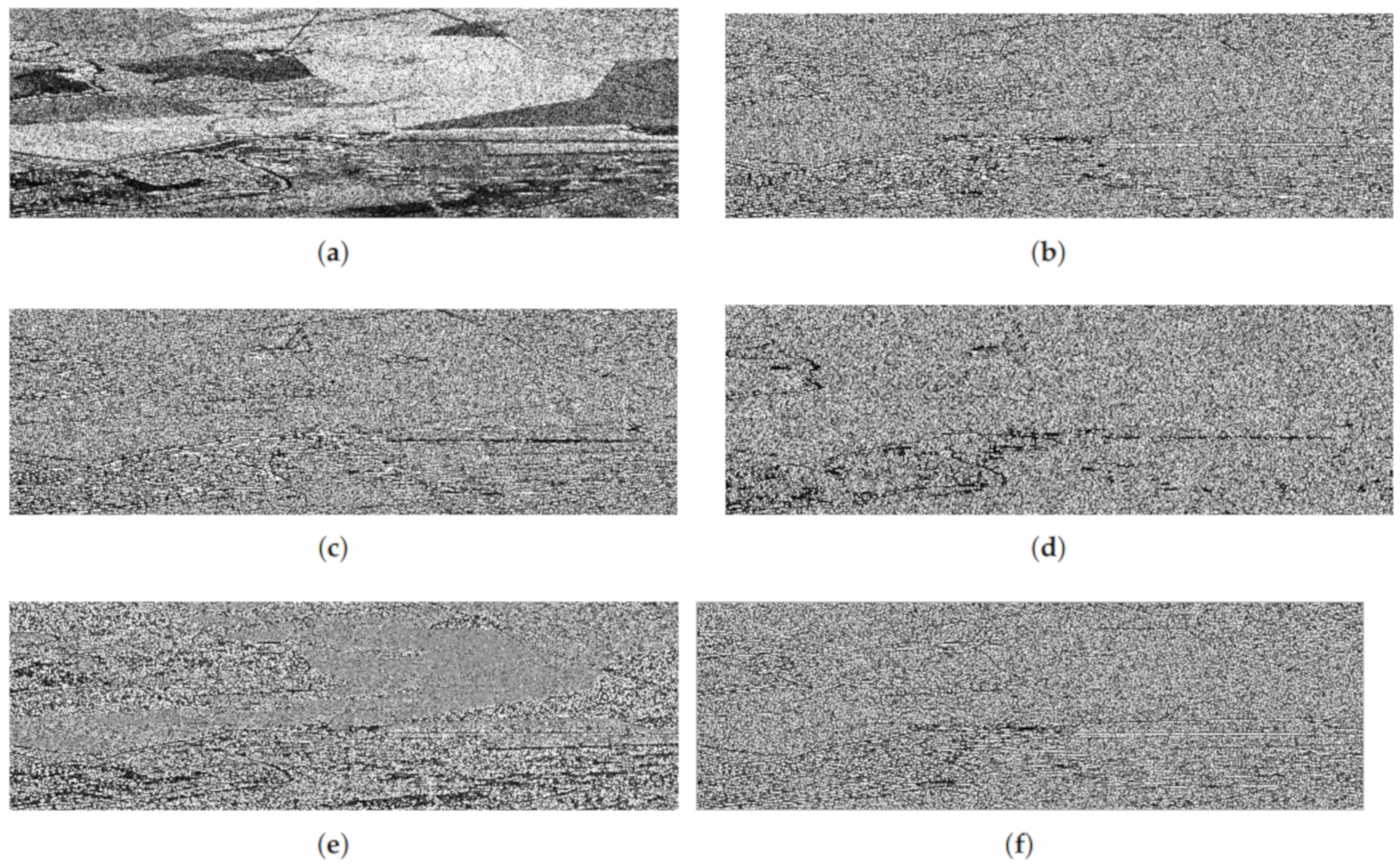
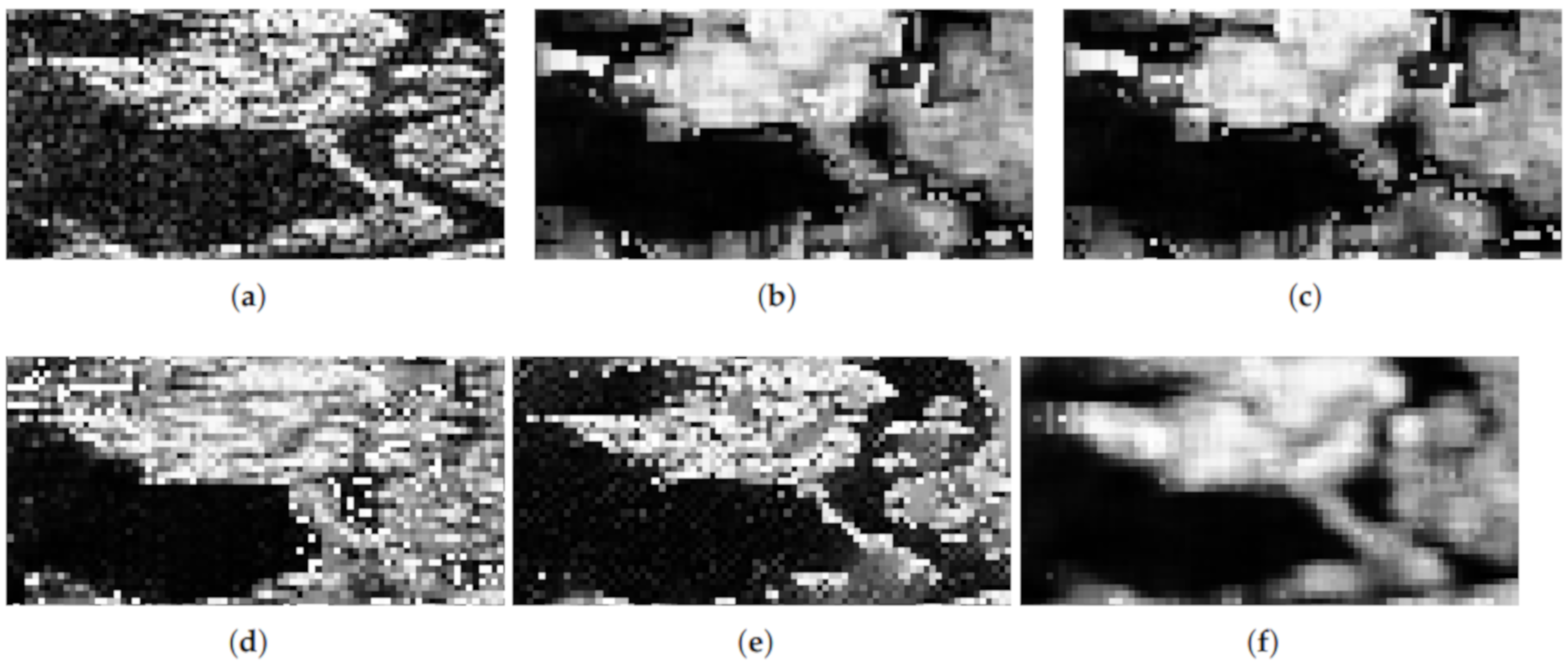
We evaluate these entropy-based non-local means filters’ performance using simulated data and an actual single-look SAR image. The new algorithm results are competitive with Lee, SRAD (Speckle Reducing Anisotropic Diffusion), and FANS (Fast Adaptive Nonlocal SAR Despeckling), and in some cases, they are better. Moreover, we show that building a non-local means filter with a proxy, as the entropy, is a feasible approach.

This article unfolds as follows. In Section 2, some properties of the ${\mathcal{G}}^0$ distribution for intensity format SAR data are recalled, which results in the ${\mathcal{G}}_I^0$ distribution. Section 3 introduces the formulae of Shannon and Rényi entropies under the ${\mathcal{G}}_I^0$ model, the asymptotic entropies distribution, and the hypothesis tests with entropies. In Section 4, the details of the proposal of entropy-based non-local means filters are explained. Section 5 presents measures for assessing the performance of speckle filters. In Section 6, the results of applying the proposed despeckling algorithm to synthetic and actual data along with the results of applying FANS (Fast Adaptive Nonlocal SAR Despeckling), Lee, and SRAD (Speckle Reducing Anisotropic Diffusion) methods are shown. We also assess their relative performance. Finally, in Section 7 some conclusions are drawn. We also assess their relative performance. Finally, in Section 7 some conclusions are drawn. Appendix A provides information about the computational platform and points at the provided code and data.

2. The ${\mathcal{G}}_{\mathbf{I}}^{\mathbf{0}}$ Distribution

Speckle noise follows a Gamma distribution, with density:

$$f_Y(y;L)=\frac{L^L}{\mathrm{\Gamma }\left(L\right)}{y}^{L-1}{e}^{-Ly},$$

denoted by $Y\sim \mathrm{\Gamma }(L,L)$. The physics of image formation imposes $L\ge 1$.

The model for the backscatter X may be any distribution with positive support. Frery et al. [28] proposed using the reciprocal gamma law, a particular case of the generalized inverse Gaussian distribution, which is characterized by the density:

$$f_X(x;\alpha ,\gamma )=\frac{{\gamma }^{-\alpha }}{\mathrm{\Gamma }(-\alpha )}{x}^{\alpha -1}{e}^{-\gamma /x},$$

where $\alpha <0$ and $\gamma >0$ are the texture and the scale parameters, respectively. Under the multiplicative model, the return $Z=XY$ follows a ${\mathcal{G}}_I^0(\alpha ,\gamma ,L)$ distribution, whose density is:

$$f_Z(z;\alpha ,\gamma )=\frac{L^L\mathrm{\Gamma }(L-\alpha )}{{\gamma }^{\alpha }\mathrm{\Gamma }(-\alpha )\mathrm{\Gamma }\left(L\right)}\frac{z^{L-1}}{{(\gamma +zL)}^{L-\alpha }},$$

(1)

where $-\alpha ,\gamma ,z>0$ and $L\ge 1$. The r-order moments of the ${\mathcal{G}}_I^0(\alpha ,\gamma ,L)$ distribution are:

$$E\left(Z^r\right)={\left(\frac{\gamma }{L}\right)}^r\frac{\mathrm{\Gamma }(-\alpha -r)}{\mathrm{\Gamma }(-\alpha )}\frac{\mathrm{\Gamma }(L+r)}{\mathrm{\Gamma }\left(L\right)},$$

(2)

provided $\alpha <-r$, and infinite otherwise. The ${\mathcal{G}}_I^0$ distribution also arises when the observation is described as a sum of a random number of returns [26,36].

We will study the noisiest case which occurs when $L=1$; it is called single-look and expression (1) becomes:

$$f_Z(z;\alpha ,\gamma )=\frac{-\alpha }{\gamma }{\left(\frac{z}{\gamma }+1\right)}^{\alpha -1}.$$

(3)

The expected value is given by:

$$E\left(Z\right)=-{\displaystyle \frac{\gamma }{\alpha +1}},\alpha <-1.$$

(4)

Chan et al. [37], using a connection between this distribution and certain Pareto laws, studied alternatives for obtaining quality samples.

We employed the maximum likelihood approach for parameter estimation. Given the sample $\mathbf{z}=(z_1,\cdots ,z_n)$ of independent and identically distributed random variables with common distribution ${\mathcal{G}}_I^0(\alpha ,\gamma ,1)$ with $(\alpha ,\gamma )\in \mathrm{\Theta }={\mathbb{R}}_{-}\times {\mathbb{R}}_{+}$, a maximum likelihood estimator of $(\alpha ,\gamma )$ satisfies:

$$(\widehat{\alpha },\widehat{\gamma })=arg\underset{(\alpha ,\gamma )\in \mathrm{\Theta }}{max}\mathcal{L}(\alpha ,\gamma ,1,\mathbf{z}),$$

(5)

where $\mathcal{L}$ is the likelihood function given by:

$$\mathcal{L}(\alpha ,\gamma ,L,\mathbf{z})={\left(\frac{L^L\mathrm{\Gamma }(L-\alpha )}{{\gamma }^{\alpha }\mathrm{\Gamma }(-\alpha )\mathrm{\Gamma }\left(L\right)}\right)}^n\prod _{i=1}^n{z}_i^{L-1}{(\gamma +L{z}_i)}^{\alpha -L}.$$

(6)

This leads to $\widehat{\alpha }$ and $\widehat{\gamma }$ such that:

$$\begin{array}{cc}\hfill n\left[{\mathrm{\Psi }}^0(-\widehat{\alpha })-{\mathrm{\Psi }}^0(1-\widehat{\alpha })\right]+\sum _{i=1}^{n}ln\frac{\widehat{\gamma }+z_i^2}{\widehat{\gamma }}& =0,\mathrm{and}\hfill \\ \hfill \frac{n\widehat{\alpha }}{\widehat{\gamma }}-(1-\widehat{\alpha })\sum _{i=1}^n\frac{1}{\widehat{\gamma }+z_i^2}& =0,\hfill \end{array}$$

where ${\mathrm{\Psi }}^0\left(t\right)=dln\mathrm{\Gamma }\left(t\right)/dt$ is the digamma function. We solved this system with numerical routines, using as an initial solution the moments estimators that stem from Equation (2) with $r=1/2,1$.

3. Entropies for the ${\mathcal{G}}_{\mathbf{I}}^{\mathbf{0}}$ Distribution

Entropy is an essential concept in information theory, related to the notion of disorder in statistics [30]. Salicrú et al. [38] proposed the $(h;\mathrm{\Phi })$-entropy class, which generalizes the original concept and facilitates the computation. In this section, the Shannon and Rényi entropies for the ${\mathcal{G}}_I^0$ distribution, in the single-look case, are computed. Let f be a probability density function with support $\mathsf{\Omega }$, and a r-dimensional parameter vector $\theta =({\theta }_1,\cdots ,{\theta }_r)\in \mathrm{\Theta }\subset {\mathbb{R}}^r$, with $\mathrm{\Theta }$ the parameter space. The $(h,\varphi )$-entropy $H_{\varphi }^h(f,\theta )$ of f is given by:

$$H_{\varphi }^h(f,\theta )=h\left[{\int }_{{\Omega }}\varphi \left(f(x,\theta )\right)dx\right],$$

(7)

being $\varphi :\left[0,+\infty \right)\to \mathbb{R}$ concave and $h:\mathbb{R}\to \mathbb{R}$ an increasing function or $\varphi :[0,+\infty )\to \mathbb{R}$ convex and $h:\mathbb{R}\to \mathbb{R}$ a decreasing function [35]. In this work we use Shannon and Rényi entropies, which are obtained making:

• Shannon entropy: $h\left(x\right)=x$ and $\varphi \left(x\right)=-xlnx$; and
• Rényi entropy: $h\left(x\right)={(1-\beta )}^{-1}lnx$ and $\varphi \left(x\right)=x^{\beta }$, with $\beta \in (0,1)$.

The Shannon entropy of a probability density function f with parameters $\theta =({\theta }_1,\cdots ,{\theta }_r)$$\in \mathrm{\Theta }\subset {\mathbb{R}}^r$ is given by:

$$H_S(f,\theta )=-{\int }_{-\infty }^{+\infty }f(z,\theta )lnf(z,\theta )dz.$$

(8)

Then, for the ${\mathcal{G}}_I^0$ distribution, considering $\theta =(\alpha ,\gamma )$ and $L=1$, using Equation (3), we have:

$$\begin{array}{cc}\hfill H_S(f_{{\mathcal{G}}_I^0},\alpha ,\gamma )& =-{\int }_0^{+\infty }-\frac{\alpha }{\gamma }{\left(1+\frac{z}{\gamma }\right)}^{\alpha -1}ln\left[-\frac{\alpha }{\gamma }{\left(1+\frac{z}{\gamma }\right)}^{\alpha -1}\right]dz\hfill \\ \hfill & =\frac{\alpha -1}{\alpha }-ln\frac{-\alpha }{\gamma },\hfill \end{array}$$

(9)

where $-\alpha ,\gamma >0$. The Rényi entropy of order $\beta$, the probability density function f is given by:

$$H_R(f,\theta ,\beta )=\frac{1}{1-\beta }ln\left({\int }_{-\infty }^{+\infty }{\left[f(z,\theta )\right]}^{\beta }dz\right),\beta \in (0,1).$$

(10)

So, for the single look ${\mathcal{G}}_I^0$ distribution, considering $\theta =(\alpha ,\gamma )$, using Equation (3), it becomes:

$$\begin{array}{cc}\hfill H_R(f_{{\mathcal{G}}_I^0},\alpha ,\gamma ,\beta )& =\frac{1}{1-\beta }ln\left({\int }_{-\infty }^{+\infty }{\left[-\frac{\alpha }{\gamma }{\left(1+\frac{z}{\gamma }\right)}^{\alpha -1}\right]}^{\beta }dz\right)\hfill \\ \hfill & =\frac{\beta }{1-\beta }ln\left(\frac{-\alpha }{\gamma }\right)+\frac{1}{1-\beta }ln\left(\frac{\gamma }{\beta (1-\alpha )+1}\right),\hfill \end{array}$$

(11)

where $-\alpha ,\gamma >0$ and the additional restriction $\alpha <-{\beta }^{-1}+1$.

3.1. Asymptotic Entropy Distribution

Pardo et al. [39] obtained the asymptotic behavior of any $H_h^{\varphi }$ entropy indexed by maximum likelihood estimators. We present here a brief explanation of this point, and any interested readers can refer to [35,39,40]. Consider a random sample of size N from the distribution characterized by the probability density function f, with support ${\Omega }$ and a r-dimensional parameter vector $\theta \in \mathrm{\Theta }\subset {\mathbb{R}}^r$, where $\mathrm{\Theta }$ is the parameter space, and the maximum likelihood estimator $\widehat{\theta }=({\widehat{\theta }}_1,{\widehat{\theta }}_2,\cdots ,{\widehat{\theta }}_r)$ of $\theta$ based on a random sample. Then, under mild regularity conditions, holds that:

$$\sqrt{N}\left(H_h^{\varphi }(f,\widehat{\theta })-H_h^{\varphi }(f,\theta )\right)\underset{N\to \infty }{\overset{D}{\to }}\mathcal{N}(0,{\sigma }_H^2\left(\theta \right)),$$

(12)

being ${\sigma }_H^2\left(\theta \right)={\delta }^{T}K{\left(\theta \right)}^{-1}\delta$, where $K\left(\theta \right)$ is the Fisher information matrix of f and $\delta$ is a vector given by:

$$\begin{array}{c}{\displaystyle {\delta }^T=\left(\begin{array}{cccc}{\delta }_1& {\delta }_2& \cdots & {\delta }_r\end{array}\right)\mathrm{with}{\delta }_i=\frac{\partial H_h^{\varphi }\left(\theta \right)}{\partial {\theta }_i},}\\ K\left(\theta \right)=E\left(-\frac{{\partial }^{2}lnf(z,\theta )}{\partial {\theta }^2}\right),\end{array}$$

(13)

and $\mathcal{N}(\mu ,\sigma )$ is the Gaussian distribution with mean $\mu$ and variance ${\sigma }^2$, and ’$\stackrel{D}{\to }$’ denotes convergence in distribution.

We derived closed formulas of the asymptotic variance for the single look ${\mathcal{G}}_I^0$ distribution, in both cases, Shannon and Rényi entropies. From Equation (3), being $f(z;\alpha ,\gamma )$ the probability density function of the ${\mathcal{G}}_I^0$,

$$lnf(z;\alpha ,\gamma )=ln(-\alpha )-ln\gamma +(\alpha -1)ln\left(1+\frac{z}{\gamma }\right),$$

(14)

where $-\alpha ,\gamma >0$. The second-order derivatives are given by:

$$\begin{array}{cc}\hfill \frac{{\partial }^{2}lnf}{\partial {\alpha }^2}& =-\frac{1}{{\alpha }^2},\hfill \end{array}$$

(15)

$$\begin{array}{cc}\hfill \frac{{\partial }^{2}lnf}{\partial \alpha \partial \gamma }& =-\frac{z}{{\gamma }^2+z\gamma },\mathrm{and}\hfill \end{array}$$

(16)

$$\begin{array}{cc}\hfill \frac{{\partial }^{2}lnf}{\partial {\gamma }^2}& ={\displaystyle \frac{1}{{\gamma }^2}}+{\displaystyle \frac{\alpha -1}{{\gamma }^2}}\left[-{\displaystyle \frac{z^2}{{(\gamma +z)}^2}}+{\displaystyle \frac{2z}{z+\gamma }}\right].\hfill \end{array}$$

(17)

Then, the Fisher information matrix for the ${\mathcal{G}}_I^0(\alpha ,\gamma ,1)$ distribution is given by:

$$K(\alpha ,\gamma )=\left(\begin{array}{cc}{\displaystyle \frac{1}{{\alpha }^2}}& {\displaystyle \frac{1}{\gamma (1-\alpha )}}\\ {\displaystyle \frac{1}{\gamma (1-\alpha )}}& {\displaystyle \frac{\alpha }{{\gamma }^2(\alpha -2)}}\end{array}\right),$$

(18)

which is a positive definite matrix, so it can be inverted:

$${\left(\begin{array}{c}K(\alpha ,\gamma )\end{array}\right)}^{-1}=\left(\begin{array}{cc}{(\alpha -1)}^2{\alpha }^2& \alpha \gamma (\alpha -1)(\alpha -2)\\ \alpha \gamma (\alpha -1)(\alpha -2)& {\alpha }^{-1}{\gamma }^2{(\alpha -1)}^2(\alpha -2)\end{array}\right).$$

(19)

We compute the asymptotic variance of the Shannon entropy from (13), (9), and (19). We have that:

$${\delta }_S^T=\left(\begin{array}{cc}{\delta }_1& {\delta }_2\end{array}\right)=\left(\begin{array}{cc}{\displaystyle \frac{\partial H_S(\alpha ,\gamma )}{\partial \alpha }}& {\displaystyle \frac{\partial H_S(\alpha ,\gamma )}{\partial \gamma }}\end{array}\right)=\left(\begin{array}{cc}{\displaystyle \frac{1}{{\alpha }^2}}-{\displaystyle \frac{1}{\alpha }}& {\displaystyle \frac{1}{\gamma }}\end{array}\right),$$

(20)

leading to:

$${\sigma }_{H_S}^2={\displaystyle \frac{{(\alpha -1)}^2\left[(-2+4{\alpha }^3-{\gamma }^2-{\alpha }^2(10+{\gamma }^2)+\alpha (5+2{\gamma }^2))\right]}{{\alpha }^2\left[\alpha (5+2{\gamma }^2)-2-{\gamma }^2-{\alpha }^2(2+{\gamma }^2)\right]}}.$$

(21)

In a similar way, for the Rényi entropy, from (11):

$${\delta }_R^T=\left(\begin{array}{cc}{\displaystyle \frac{\partial H_R(\alpha ,\gamma )}{\partial \alpha }}& {\displaystyle \frac{\partial H_R(\alpha ,\gamma )}{\partial \gamma }}\end{array}\right)=\left(\begin{array}{cc}{\displaystyle \frac{\beta }{1-\beta }}\left({\displaystyle \frac{1}{\alpha }}-{\displaystyle \frac{1}{\beta (\alpha -1)+1}}\right)& {\displaystyle \frac{1}{\gamma }}\end{array}\right),$$

(22)

which results in:

$$\begin{array}{c}{\sigma }_{H_R^{\beta }}^2={\displaystyle \frac{{(\alpha -1)}^2\left[-2+4\beta +4{\alpha }^3{\beta }^2-{\beta }^2(4+{\gamma }^2)\right]}{{\left[1+(\alpha -1)\beta \right]}^2\left[\alpha (5+2{\gamma }^2)-{\alpha }^2(2+{\gamma }^2)-{\gamma }^2-2\right]}}+\\ \frac{\alpha \left[1-10\beta +2{\beta }^2\left(7+{\gamma }^2-{\alpha }^2\beta (-4+\beta (14+{\gamma }^2))\right)\right]}{{\left(1+(\alpha -1)\beta \right)}^2\left(\alpha (5+2{\gamma }^2)-{\alpha }^2(2+{\gamma }^2)-{\gamma }^2-2\right)}.\end{array}$$

(23)

The Fisher information matrix, which is involved in computing both ${\sigma }_{H_S}^2$ and ${\sigma }_{H_R^{\beta }}^2$, is invertible, but it can be ill-conditioned. Writing:

$$\begin{array}{cc}\hfill a& =\frac{1}{{\alpha }^2},\hfill \end{array}$$

(24)

$$\begin{array}{cc}\hfill b& =\frac{1}{\gamma (1-\alpha )},\mathrm{and}\hfill \end{array}$$

(25)

$$\begin{array}{cc}\hfill c& =\frac{\alpha }{{\gamma }^2(\alpha -2)},\hfill \end{array}$$

(26)

then we have its eigenvalues given by:

$${\lambda }_{1,2}=\frac{(a+c)\pm \sqrt{{(a-c)}^2+4b^2}}{2},$$

which are real numbers. Figure 1 shows the values of eingenvalues of the Fisher information matrix for several values of $\alpha$ and $\gamma$ parameters, and $L=1$. Figure 1a,b show the first and second eigenvalues, respectively. It can be observed that the second eigenvalue tends to zero as $\alpha \to -\infty$ for all values of $\gamma$ and then, the matrix inversion becomes unstable for textureless areas, regardless of scale. Frery et al. [41] noticed that maximum likelihood estimates were unstable in some areas of the parameter space and analyzed this issue from the sample size viewpoint.

Figure 1. Plots of the first and second eigenvalues of the Fisher information matrix for several values of $\alpha$ and $\gamma$, $L=1$. (a) First eigenvalue and (b) second eigenvalue.

Such behavior explains why maximum likelihood estimation is numerically unstable in textureless areas, i.e., where the mean number of backscatterers is huge.

3.2. Hypothesis Testing Based on h-$\varphi$ Entropies

Entropies are widely used as feature discrimination [40,42]. In this section, a hypothesis test based on Shannon and Rényi entropies is built. Let $X=\{x_1,\cdots ,x_{N_1}\}$ and $Y=\{y_1,\cdots ,y_{N_2}\}$ be two random samples of sizes $N_1$ and $N_2$, respectively, from the ${\mathcal{G}}_I^0(\alpha ,\gamma ,1)$ distribution and parameters $({\alpha }_1,{\gamma }_1)$ and $({\alpha }_2,{\gamma }_2)$, respectively. We are interested in testing the following hypotheses:

$$\begin{array}{cc}\hfill H_0& :H_{\mathcal{M}}({\alpha }_1,{\gamma }_1)=H_{\mathcal{M}}({\alpha }_2,{\gamma }_2)=v,\hfill \\ \hfill H_1& :H_{\mathcal{M}}({\alpha }_1,{\gamma }_1)\ne H_{\mathcal{M}}({\alpha }_2,{\gamma }_2).\hfill \end{array}$$

(27)

That means, statistical evidence that two random samples have the same entropy is sought or in other words, if the diversity of two independent random samples is equal. Let $({\widehat{\alpha }}_i,{\widehat{\gamma }}_i),i=1,2$. be the maximum likelihood estimator of $({\alpha }_i,{\gamma }_i),i=1,2$. Following the result of Equation (12)  (see [35]) and for a parameter vector of dimension 2, the test statistic has known asymptotic distribution:

$$\frac{\sqrt{N_i}\left(H_{\mathcal{M}}({\widehat{\alpha }}_i,{\widehat{\gamma }}_i)-v\right)}{{\sigma }_{\mathcal{M}}({\widehat{\alpha }}_i,{\widehat{\gamma }}_i)}\underset{N_i\to \infty }{\overset{D}{\to }}\mathcal{N}(0,1),i=1,2$$

(28)

Therefore,

$$\sum _{i=1}^2\frac{N_i{\left(H_{\mathcal{M}}({\widehat{\alpha }}_i,{\widehat{\gamma }}_i)-v\right)}^2}{{\sigma }_{\mathcal{M}}^2({\widehat{\alpha }}_i,{\widehat{\gamma }}_i)}\underset{N_i\to \infty }{\overset{D}{\to }}{\chi }_2^2,$$

(29)

but v is unknown, then the Cochran’s theorem [43] can be applied to obtain:

$$\sum _{i=1}^2\frac{N_i{\left(H_{\mathcal{M}}({\widehat{\alpha }}_i,{\widehat{\gamma }}_i)-v\right)}^2}{{\sigma }_{\mathcal{M}}^2({\widehat{\alpha }}_i,{\widehat{\gamma }}_i)}=\sum _{i=1}^2\frac{N_i{\left(H_{\mathcal{M}}({\widehat{\alpha }}_i,{\widehat{\gamma }}_i)-\overline{v}\right)}^2}{{\sigma }_{\mathcal{M}}^2({\widehat{\alpha }}_i,{\widehat{\gamma }}_i)}+\sum _{i=1}^2\frac{N_i(v-\overline{v})}{{\sigma }_{\mathcal{M}}^2({\widehat{\alpha }}_i,{\widehat{\gamma }}_i)},$$

(30)

being,

$$\overline{v}={\left[\sum _{i=1}^2\frac{N_i}{{\sigma }_{\mathcal{M}}^2({\widehat{\alpha }}_i,{\widehat{\gamma }}_i)}\right]}^{-1}\sum _{i=1}^2\frac{N_i{H}_{\mathcal{M}}({\widehat{\alpha }}_i,{\widehat{\gamma }}_i)}{{\sigma }_{\mathcal{M}}^2({\widehat{\alpha }}_i,{\widehat{\gamma }}_i)}.$$

(31)

Since the second term of the right side of Equation (30) is ${\chi }_1^2$ distributed and the left side of the Equation (30) is ${\chi }_2^2$ distributed, we conclude that:

$$\sum _{i=1}^2\frac{N_i{\left(H_{\mathcal{M}}({\widehat{\alpha }}_i,{\widehat{\gamma }}_i)-\overline{v}\right)}^2}{{\sigma }_{\mathcal{M}}^2({\widehat{\alpha }}_i,{\widehat{\gamma }}_i)}\underset{N_i\to \infty }{\overset{D}{\to }}{\chi }_1^2,$$

(32)

where $\mathcal{M}\in \{S,R\}$ are S and R, the Shannon and Rényi entropy, respectively. We are interested in compare samples of same size $N_1=N_2=N$ then, the test statistic reduces to (see [38,44]):

$$S_{\mathcal{M}}\left(({\widehat{\alpha }}_1,{\widehat{\gamma }}_1),({\widehat{\alpha }}_2,{\widehat{\gamma }}_2)\right)=N\frac{{\left(H_{\mathcal{M}}({\widehat{\alpha }}_1,{\widehat{\gamma }}_1)-H_{\mathcal{M}}({\widehat{\alpha }}_2,{\widehat{\gamma }}_2)\right)}^2}{{\sigma }_{\mathcal{M}}^2({\widehat{\alpha }}_1,{\widehat{\gamma }}_1)+{\sigma }_{\mathcal{M}}^2({\widehat{\alpha }}_2,{\widehat{\gamma }}_2)}.$$

(33)

Then, the null hypothesis can be rejected with significance level $\eta$ if:

$$P({\chi }_1^2>s)\le \eta ,$$

(34)

where s is the observed test statistic. The p-value is $P({\chi }_1^2>s)$, $\mathcal{M}\in \left\{S,R\right\}$.

4. Speckle Reduction by Comparing Entropies

The proposed method for despeckling images is based on testing whether two random samples ${\mathbf{z}}_1\sim {\mathcal{G}}_I^0({\alpha }_1,{\gamma }_1,1)$ and ${\mathbf{z}}_2\sim {\mathcal{G}}_I^0({\alpha }_2,{\gamma }_2,1)$ have the same diversity. We then compare the Shannon and Rényi entropies, which are scalars that depend on the parameters.

Non-local means filters use a large convolution mask of size $d\times d$ with $d=2*n+1$, $n=1,2,\cdots$ taking an average of all pixels in the mask, weighted by a similarity measure between these pixels and the center of the mask.

Let Z be the noisy image of size $m\times m$, then the filtered image $\widehat{X}$ in position $(x,y)$ is given by:

$$\widehat{X}(x,y)=\frac{{\sum }_{i=x-n}^{x+n}{\sum }_{j=y-n}^{y+n}Z(x+i,y+j)w(i,j)}{{\sum }_{i=x-n}^{x+n}{\sum }_{j=y-n}^{y+n}w(i,j)},$$

(35)

where $\widehat{X}$ estimates the noiseless image X, and $w(i,j)$$i,j=1,\cdots ,d$ are the weights.

In our proposal, we build an image filter by computing the mask w in each step of the algorithm, using the test statistic from Equation (27) with significance level $\eta$. For simplicity, we will describe the implementation using square windows, but the user may consider any shape. We defined two sets: The search and the estimation windows. The search window ${\mathbf{W}}_i$ has fixed size $n\times n$ and is centered on every pixel $i=1,\cdots ,m^2$. 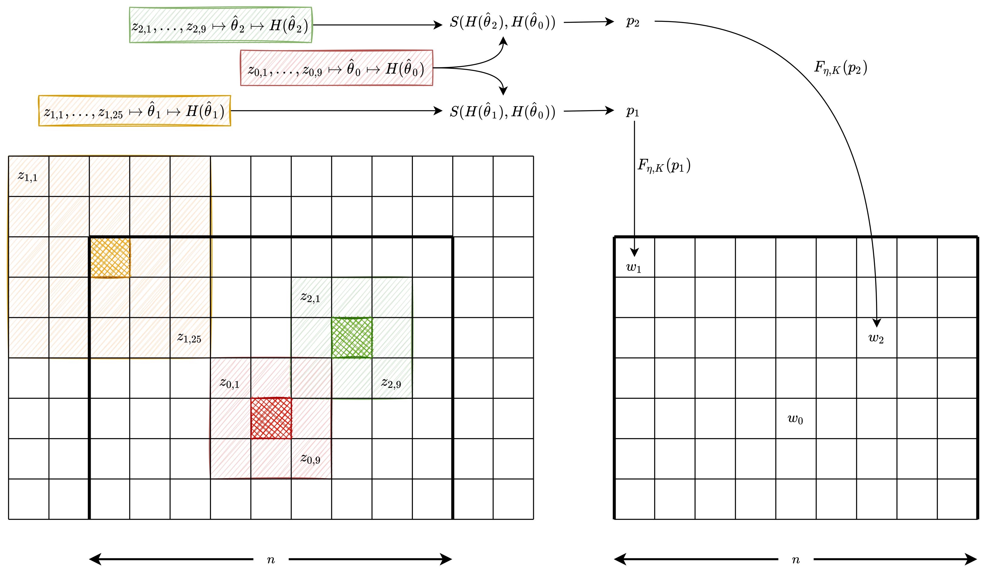At every location of this search window, we define estimation patches around each pixel. These windows may vary in size, e.g., in an adaptive scheme.

Figure 2 illustrates an instance of such implementation with $n=9$. The left grid represents the image, while the right grid shows the mask that will be applied to the central pixel (identified in red cross-hatch).

Figure 2. Left: Search window and estimation patches. Right: Resulting convolution mask to be applied on the search window to compute a single filtered value corresponding to the central pixel (cross-hatched in red).

The central pixel is identified with red cross-hatch, and its estimation window has size $3\times 3$; denote these observations as ${\mathbf{z}}_0=(z_{0,1},z_{0,2},\cdots ,z_{0,9})$. We also show two estimations windows; those corresponding to the pixels identified with orange and green cross-hatches and have, respectively, dimensions $5\times 5$ and $3\times 3$, and their observations are ${\mathbf{z}}_1=(z_{1,1},z_{1,2},\cdots ,z_{1,25})$ and ${\mathbf{z}}_2=(z_{2,1},z_{2,2},\cdots ,z_{2,9})$, respectively.

We compare the pairwise diversities of the samples ${\mathbf{z}}_j$, $j=1,2$, summarized as $S\left(H\left({\widehat{\theta }}_0\right),H\left({\widehat{\theta }}_0\right)\right)$ in Figure 2, with respect to ${\mathbf{z}}_0$ estimating by maximum likelihood the parameters $(\alpha ,\gamma )$ from the ${\mathcal{G}}_I^0$ distribution. We obtain $({\widehat{\alpha }}_0,{\widehat{\gamma }}_0)$ from ${\mathbf{z}}_0$, $({\widehat{\alpha }}_1,{\widehat{\gamma }}_1)$ from ${\mathbf{z}}_1$, and $({\widehat{\alpha }}_2,{\widehat{\gamma }}_2)$ from ${\mathbf{z}}_2$; this step is summarized as ${\mathbf{z}}_j\mapsto {\widehat{\theta }}_j$ in Figure 2. Then, both the Shannon and Rényi entropies are estimated (summarized as ${\widehat{\theta }}_j\mapsto H\left({\widehat{\theta }}_j\right)$) and the test statistic is obtained. The weight $w_1$ ($w_2$ respectively) stems from comparing the samples ${\mathbf{z}}_0$ (${\mathbf{z}}_2$ respectively) and ${\mathbf{z}}_0$. Finally, we transform the observed p-values in the weights $w_1$ and $w_2$ by using a smoothing function.

Each p-value may be used directly as a weight w but, as discussed by Torres et al. [21], such a choice introduces a conceptual distortion. Consider, for instance, the samples ${\mathbf{z}}_1$ and ${\mathbf{z}}_2$. Assume that, when contrasted with the central sample ${\mathbf{z}}_0$, they produce the p-values $p_1=0.05$ and $p_2=0.93$. In this case, the first weight will be significantly smaller than the second one, whereas there is no evidence to reject any of the samples at level $\eta =0.05$. Torres et al. [21] proposed using a piece-wise linear function that maps all values above $\eta$ to 1, a linear transformation of values between $\eta /2$ and $\eta$, and zero below $\eta /2$. 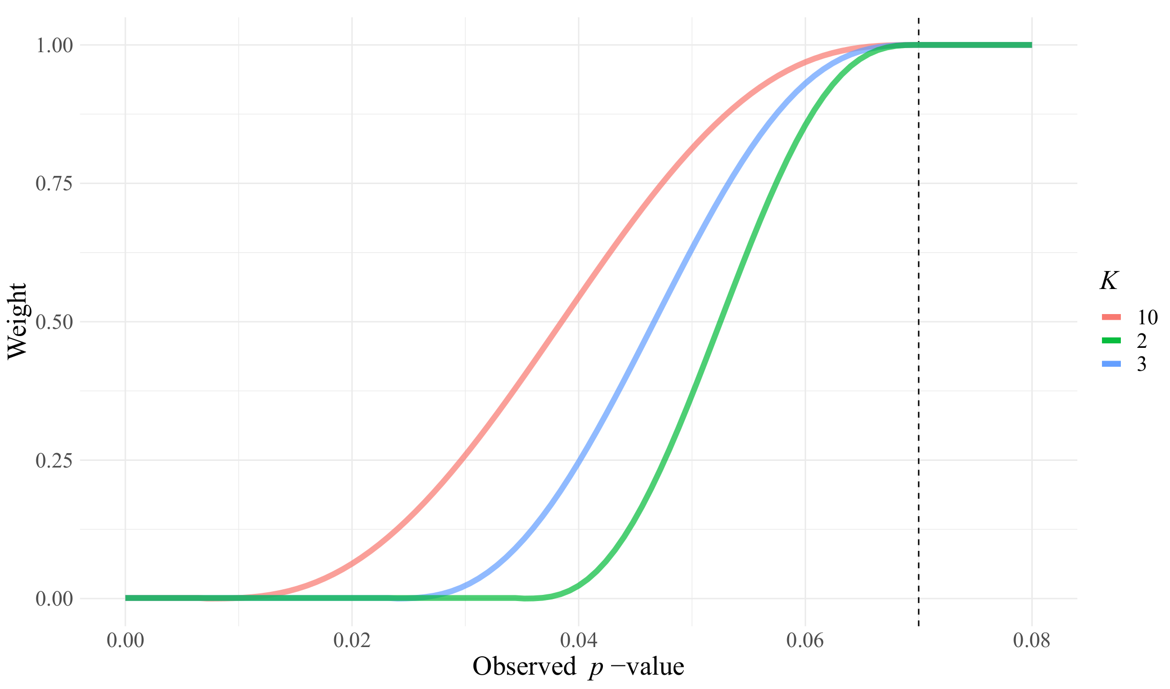In this work, we propose a smooth activating function with zero first- and second-order derivatives at the inflexion points. The “smoother step function” defined by Ebert [45] is given as:

$$f_{\mathrm{smoother}}\left(x\right)=\left\{\begin{array}{cc}0\hfill & \mathrm{if}x<0,\hfill \\ 6x^5-15x^4+10x^3\hfill & \mathrm{if}0\le x\le 1,\hfill \\ 1\hfill & \mathrm{if}x>1.\hfill \end{array}\right.$$

(36)

This function connects in a smooth manner the points $(0,0)$ and $(1,1)$. We modify $f_{\mathrm{smoother}}$ in order to connect $(\eta /K,0)$ and $(\eta ,1)$, for every $K\in \mathbb{N}$, and define the weight w as a function of the observed p-value as the result of the following activating function:

$$F_{\eta ,K}\left(p\right)=f_{\mathrm{smoother}}\left(\frac{p-\eta /K}{\eta -\eta /K}\right).$$

(37)

This function is zero for $p<\eta /K$, and is one above $\eta$. The parameter K controls the transformation’s steepness, as shown in Figure 3. From our experiments, we recommend $K=3$.

Figure 3. Transformation between p-values and weights for $\eta =0.07$ and $K\in \{2,3,10\}$.

Algorithm 1 shows the steps of the method.

Algorithm 1 Despeckling by similarity of entropies.

1: Input: Original noisy image Z of size $m\times m$, d, k, $d>k$ sizes of the large and small sliding windows, respectively 2: for$i=1$$m^2$do 3:    Consider a sliding window ${\mathbf{W}}_i$ of size $n\times n$ around pixel i 4:    Let $z_0^i$ be the central pixel of ${\mathbf{W}}_i$ 5:    Consider a $k\times k$ neighborhood of $z_0^i$, named $W_i^0$ 6:    Compute the maximum likelihood parameter estimates of the ${\mathcal{G}}_I^0$ parameters, $({\widehat{\alpha }}_i^0,{\widehat{\gamma }}_i^0)$, the entropy and the asymptotic variance for the sample $W_i^0$ 7:    for $j=1$ $d^2$ do 8:      Consider $W_i^j$, patches of size $k\times k$ inside the large window ${\mathbf{W}}_i$, corresponding to the neighborhoods of each pixel $z_j\in {\mathbf{W}}_i$, as Figure 2 shows 9:      Compute the estimates $({\widehat{\alpha }}_i^j,{\widehat{\gamma }}_i^j)$, the entropy, and its asymptotic variance of the sample $W_i^j$ 10:      Compute the statistic $S_i^j$, using Equation (33), and $p_i^j$, its p-value using its asymptotic distribution ${\chi }_1^2$ 11:      Compute the (yet to be normalized) weight $w_i^j=F_{\eta ,K}\left(p_j^i\right)$ 12:    end for 13:    Divide all the weights by ${\sum }_{j=1}^{d^2}{w}_i^j$ 14:    Compute the estimated noiseless observation ${\widehat{x}}_i={\sum }_{n\in W_i^j}{w}_i^n{z}_i$ 15: end for 16: return ${\widehat{x}}_i$, $i=1,\cdots ,m^2$

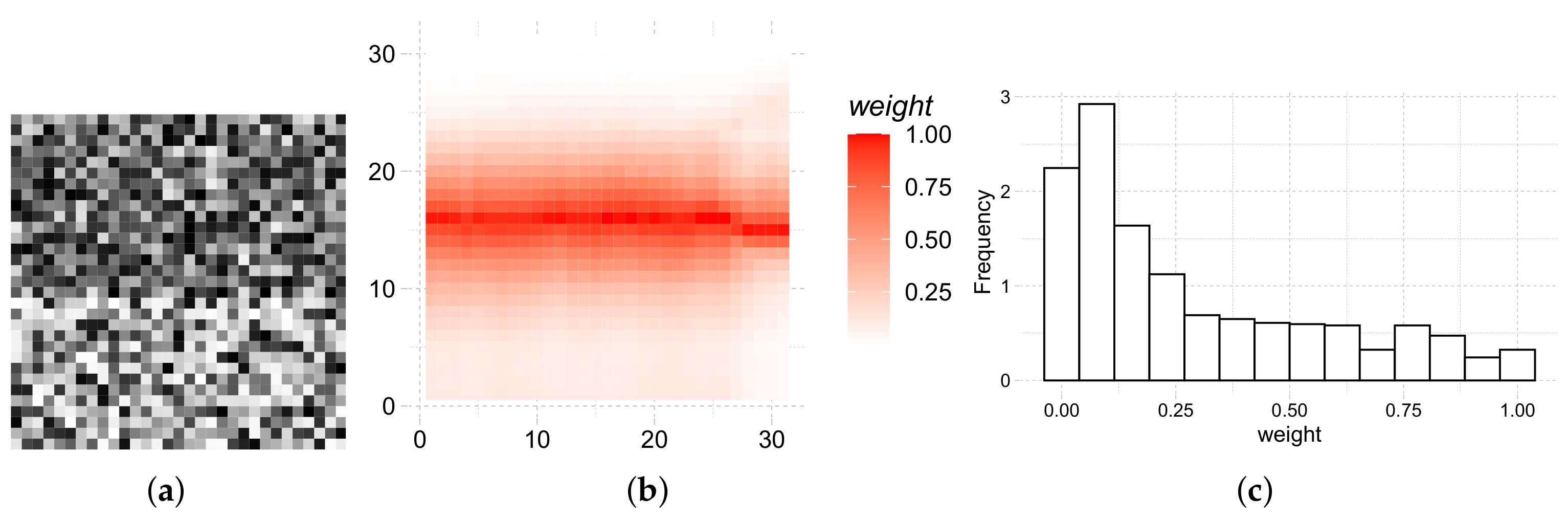
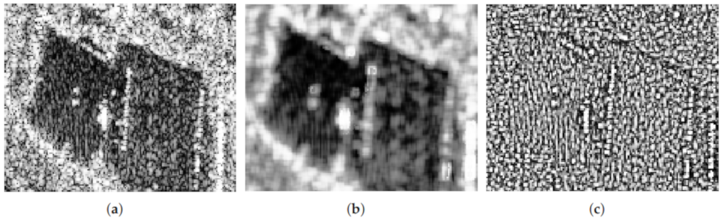
Figure 4 shows the heatmap and histogram of the weights of a sliding window over an edge of the original image. Figure 4a shows the cropping of the image where the weights were computed. Observations on the edge, and close to it have a strong influence on the filtered data, while those far or with a different underlying distribution weigh less.

Figure 4. Original image patch, heat map, and histogram of weights over an edge, before normalization. (a) Original data. (b) Heat map. (c) Histogram of weights.

5. Filter Quality

We used the ratio image, which is the point to point division between the noisy image and the filtered image, to measure noise reduction quality. It is given by $I=Z/\hat{X}$, where Z and $\hat{X}$ are the original and filtered images, respectively. Under the multiplicative model, the perfect filter produces a ratio image I which is pure speckle, i.e., a collection of independent and identically $\mathrm{\Gamma }(1,1)$ distributed random variables, with no presence of patterns or geometric structures.

5.1. First-Order Statistic

The first-order statistic component of the quality measure employs the equivalent number of looks and the mean value over homogeneous areas of the original and filtered images. An effective despeckling method should increase the equivalent number of looks and preserve the mean value. Given a textureless and homogeneous image area with sample mean $\widehat{\mu }$ and sample standard deviation $\widehat{\sigma }$, the equivalent number of looks can be estimated as $\widehat{\mathrm{ENL}}={\widehat{\mu }}^2/{\widehat{\sigma }}^2$. We automatically select N small homogeneous areas $A_i,1\le i\le N$, then the ENL residual for each area $A_i$, is estimated:

$$r_{\widehat{\mathrm{ENL}}}\left(i\right)={\displaystyle \frac{|{\widehat{\mathrm{ENL}}}_Z\left(i\right)-{\widehat{\mathrm{ENL}}}_I\left(i\right)|}{{\widehat{\mathrm{ENL}}}_Z\left(i\right)}},i=1,\cdots ,N,$$

(38)

where ${\widehat{\mathrm{ENL}}}_Z\left(i\right)$ and ${\widehat{\mathrm{ENL}}}_I\left(i\right)$ are the estimated ENL taking the sample from $A_i$ for the original image Z and the ratio image I, respectively. The relative residual due to deviations from the ideal mean, which is 1, is:

$$r_{\widehat{\mu }}\left(i\right)=|1-{\widehat{\mu }}_I\left(i\right)|,i=1,\cdots ,N,$$

(39)

where ${\widehat{\mu }}_I\left(i\right)$ is the mean value for the region $A_i$ in the ratio image. The first-order residual is the sum of those two quantities:

$$r_{\widehat{\mathrm{ENL}},\widehat{\mu }}={\displaystyle \frac{1}{2N}}\sum _{i=1}^N\left(r_{\widehat{\mathrm{ENL}}}\left(i\right)+r_{\mu }\left(i\right)\right).$$

(40)

The perfect filter would produce $r_{\widehat{\mathrm{ENL}},\widehat{\mu }}=0$.

5.2. Second-Order Statistic

The remaining geometrical content in the ratio image I is measured with the homogeneity value from Haralik’s co-occurrence matrices [46], which is given by:

$$h=\sum _{i=1}^M\sum _{j=1}^M{\displaystyle \frac{1}{1+{(i-j)}^2}}p(i,j),$$

(41)

where $p(i,j)$ is the $(i,j)$-th element of the co-occurrence matrix of size $M\times M$. The coefficient h is computed under the null hypothesis, which implies that the probability distribution of the ratio image I is invariant under random permutations. Then, if there is no structure in I, h will not change after permutations.

Let $h_0$ be the homogeneity of the original ratio image I, $h_m,1\le m\le g$ the homogeneity of the m-th permutation of I, and g the total amount of permutations. The absolute value of the relative variation of $h_0$, in percentage can be used as a measure of a distance from the null hypothesis and is given by:

$${\delta }_h=100\left|{\displaystyle \frac{h_0-{\overline{h}}_g}{h_0}}\right|,$$

(42)

where ${\overline{h}}_g=g^{-1}{\sum }_{m=1}^g{h}_m$. As ${\delta }_h$ increases, the larger the geometric structure that will remain in the radio image. Finally, the statistic to measure filter quality proposed in [25] combines ${\delta }_h$ and $r_{\widehat{\mathrm{ENL}},\widehat{\mu }}$ in the following way:

$${\mathcal{M}}_0=r_{\widehat{\mathrm{ENL}},\widehat{\mu }}+{\delta }_h.$$

(43)

The ideal filter produces ${\mathcal{M}}_0=0$, and the lack of quality of a filter can be measured by the observed value of $\mathcal{M}$.

6. Results

In this section, we present the results of applying the proposed filters. We also evaluate them using the metric presented in Section 5. Three of the most successful despeckling methods are SRAD (Speckle Reducing Anisotropic Diffusion) [15], Enhanced Lee [8], and FANS (Fast Adaptive Nonlocal SAR Despeckling) [16] algorithms. We compare their efficiency with the performance of the entropy-based filters. In all cases, the images are equalized for improved visualization.

6.1. Simulated Data

In this Section we present results of applying the filters to simulated data. We consider two phantoms: One with large areas (Figure 5), and another with strips of varying width (Figure 6). The observations deviate from the ${\mathcal{G}}_I^0$ distribution, obtained according to the recommendations presented in [37].

Figure 5. Simulated image generated with ${\mathcal{G}}_I^0(-4,10,1)$, ${\mathcal{G}}_I^0(-4,1,1)$, ${\mathcal{G}}_I^0(-1.5,10,1)$, and ${\mathcal{G}}_I^0(-1.5,1,1)$ laws (top-left, top-right, bottom-left, and bottom-right, respectively), and the result of applying the filters based on Shannon entropy, on Rényi entropy, and with the SRAD (Speckle Reducing Anisotropic Diffusion), Enhanced Lee, and FANS (Fast Adaptive Nonlocal SAR despeckling) filters. (a) Original image. (b) Shannon entropy-filtered image. (c) Rényi entropy-filtered image, $\beta =0.75$. (d) SRAD (Speckle Reducing Anisotropic Diffusion)-filtered image. (e) Lee-filtered image. (f) FANS (Fast Adaptive Nonlocal SAR Despeckling)-filtered image.

Figure 6. Results of applying the proposed filters to the background and stripes image. (a) Phantom image. (b) Shannon entropy filter.

Figure 5 is adequate for assessing the filter performance on large areas. Figure 5a shows the original data, each half of the top of the image was generated with ${\mathcal{G}}_I^0(-4,10,1)$ and ${\mathcal{G}}_I^0(-4,1,1)$ distributions, respectively. Each half of the bottom of the image was generated with ${\mathcal{G}}_I^0(-1.5,10,1)$ and ${\mathcal{G}}_I^0(-1.5,1,1)$ distributions, respectively. Figure 5b shows the filtered image using the Shannon entropy with patches of size $7\times 7$, a sliding window of size $11\times 11$, $\eta =0.15$ and $K=3$. Figure 5c shows the filtered image with Rényi entropy and $\beta =0.75$, patches of size $7\times 7$, a sliding window of size $11\times 11$, $\eta =0.15$, and $K=3$. Table 1 shows the ENL (Equivalent Number of Looks) estimates and the mean value for the original and smoothed images. Figure 5d–f show the results of applying SRAD (Speckle Reducing Anisotropic Diffusion), Enhanced Lee, and FANS (Fast Adaptive Nonlocal SAR Despeckling) filters.

Table 1. Estimates of the ENL (Equivalent Number of Looks) and mean value for images from Figure 5.

Figure	$\widehat{\mathbf{ENL}}$	$\widehat{\mathit{\mu }}$
Figure 5a	$0.53$	$5.48$
Figure 5b	$12.51$	$5.47$
Figure 5c	$13.09$	$5.53$
Figure 5d	$115.92$	$0.00031$
Figure 5e	$210.37$	$61.61$
Figure 5f	$27.71$	$61.74$

Table 1 shows that the estimated ENL increases, while the mean is almost the same.

Table 2 shows the evaluation metrics for each filter. The best method for each metric is highlighted with a gray background. It can be observed that the metric values for the proposed filters are competitive, and the Shannon entropy-based filter is the winner.

Table 2. Filter evaluation metrics for the image of Figure 5a.

Filter	${\mathit{r}}_{\widehat{\mathit{\mu }},\widehat{\mathbf{ENL}}}$	${\mathit{h}}_0$	${\overline{\mathit{h}}}_{\mathit{g}}$	${\mathit{\delta }}_{\mathit{h}}$	${\mathcal{M}}_0$
SRAD	$1.620$	$0.497$	$0.470$	$5.397$	$7.017$
Enhanced Lee	$0.128$	$0.544$	$0.541$	$0.503$	$0.631$
FANS	$0.567$	$0.177$	$0.174$	$1.945$	$2.512$
Shannon Entropy	$0.112$	$0.919$	$0.920$	$0.113$	$0.226$
Rényi Entropy	$0.155$	$0.899$	$0.901$	$0.173$	$0.328$

Figure 7 shows, in a semilogarithmic scale, the pixels values of one column of the original (orange) and filtered (light blue) images for a Shannon entropy-based method (Figure 7a) and Rényi entropy-based method (Figure 7b). The horizontal black straight lines are the theoretical mean of the data computed using Equation (4). Each plot shows two sets of boxplots: One pair to the left, corresponding to the original (orange) and filtered (light blue) values in the darker half of the image, and another pair to the right showing a summary of the original and filtered values in the brighter half. The effect of the filter is noticeable: The spread of the data is reduced, while the transition between halves is sharp, i.e., there is little blurring.

Figure 7. One column image data for the original, Shannon entropy, and Rényi entropy-filtered images. The black horizontal straight lines are the theoretical mean values of the data, in orange the original data, and in light blue the filtered data. (a) Original and Shannon smoothed images. (b) Original and Rényi smoothed images.

Figure 6 shows the results of applying the proposed filters to a phantom image which is adequate for assessing the performance on relatively small features. This phantom was proposed by Gomez et al. [47].

The image has $500\times 500$ pixels, and is divided in four blocks: Upper left, upper right, bottom left, and bottom right. Table 3 shows the background and stripes parameters in each block. Notice that in the left half the background and stripes have the same mean value. This is a challenging situation for any filter.

Table 3. Parameters of the simulated data in Figure 6a.

		Left		Right
		$\mathbf{\alpha }$	$\mathbf{\gamma }$	$\mathbf{\alpha }$	$\mathbf{\gamma }$
Top	Background	$-2$	1	$-2$	5
	Stripes	$-10$	9	$-2$	50
Bottom	Background	$-3$	20	$-3$	10
	Stripes	$-9$	80	$-6$	250

The ability of the filter based on the Shannon entropy to distinguish areas with the same mean but different roughness is noticeable in Figure 6. The edges between areas are also well preserved. For the sake of brevity, we omit the results produced by the filter based on the Rényi entropy, because they are similar.

Table 4 and Table 5 show the estimated ENL, mean values, and evaluation metrics for these images. It can be observed the filter ability to increase the equivalent number of looks while preserving the mean value.

Table 4. Estimates of the ENL and mean value for images from Figure 6.

Figure	$\widehat{\mathbf{ENL}}$	$\widehat{\mathit{\mu }}$
Figure 6a	$0.45$	$1.3$
Figure 6b	$20.05$	$1.12$

Table 5. Filter evaluation metrics for the actual data of Figure 6.

Filter	${\mathit{r}}_{\widehat{\mathit{\mu }},\widehat{\mathbf{ENL}}}$	${\mathit{h}}_0$	${\overline{\mathit{h}}}_{\mathit{g}}$	${\mathit{\delta }}_{\mathit{h}}$	${\mathcal{M}}_0$
Shannon Entropy	$0.05$	$0.9223$	$0.9238$	$0.16$	$0.210$
Rényi Entropy	$0.11$	$0.927$	$0.928$	$0.15$	$0.270$

6.2. Data from Actual Sensors

Figure 8 shows the results of applying the despeckling method to actual data. Figure 8a corresponds to the original image. Figure 8b,c are the results of applying the despeckling method with Shannon entropy and with Rényi entropy, respectively. The used parameters are: $n=11$, $k=7$, $\eta =0.15$, $\beta =0.75$, and $K=3$.

Figure 8. Original image and filtered version with the Shannon entropy, Rényi entropy, FANS (Fast Adaptive Nonlocal SAR Despeckling), SRAD (Speckle Reducing Anisotropic Diffusion) and Enhanced Lee filters. (a) Original HH (Horizontal-Horizontal polarization) data. (b) Smoothed image with the Shannon entropy. (c) Smoothed image with the Rényi entropy $\beta =0.75$. (d) Smoothed image with the FANS (Fast Adaptive Nonlocal SAR Despeckling) filter. (e) Smoothed image with the SRAD (Speckle Reducing Anisotropic Diffusion) filter. (f) Smoothed image with the Enhanced-Lee filter.

Figure 8d shows the result of applying the FANS (Fast Adaptive Nonlocal SAR Despeckling) filter, Figure 8e shows the SRAD (Speckle Reducing Anisotropic Diffusion) filter, and Figure 8f shows the Lee filter. Figure 9 shows the ratio images; Figure 8b–f correspond to Shannon entropy, Rényi entropy, FANS (Fast Adaptive Nonlocal SAR Despeckling), as well as SRAD (Speckle Reducing Anisotropic Diffusion) and Lee filters, respectively.

Figure 9. Original and ratio images. (a) Original HH (Horizontal-Horizontal polarization) data. (b) Ratio image from the Shannon entropy filter. (c) Ratio image from the Rényi entropy filter. (d) Ratio image from the FANS (Fast Adaptive Nonlocal SAR Despeckling) filter. (e) Ratio image from the SRAD (Speckle Reducing Anisotropic Diffusion) filter. (f) Ratio image from the Lee filter.

Table 6 and Table 7 show the estimated ENL, mean values, and evaluation metrics for these images. Note the filter ability to increase the equivalent number of looks while preserving the mean value.

Table 6. Estimates of the ENL and mean value for images from Figure 8.

Figure	$\widehat{\mathbf{ENL}}$	$\widehat{\mathit{\mu }}$
Figure 8a	$0.495$	$0.0016$
Figure 8b	$7.056$	$0.0013$
Figure 8c	$0.745$	$0.0015$
Figure 8d	$0.38$	$0.011$
Figure 8e	$2.92$	$0.0015$
Figure 8f	$10.55$	$0.003$

Table 7. Filter evaluation metrics for the actual data of Figure 8.

Filter	${\mathit{r}}_{\widehat{\mathit{\mu }},\widehat{\mathbf{ENL}}}$	${\mathit{h}}_0$	${\overline{\mathit{h}}}_{\mathit{g}}$	${\mathit{\delta }}_{\mathit{h}}$	${\mathcal{M}}_0$
SRAD	$81.412$	$0.999$	$0.999$	$0.002$	$81.414$
Enhanced Lee	$0.206$	$0.550$	$0.546$	$0.675$	$0.880$
FANS	$0.535$	$0.211$	$0.195$	$7.561$	$8.096$
Shannon Entropy	$0.392$	$0.997$	$0.996$	$0.185$	$0.411$
Rényi Entropy	$0.387$	$0.997$	$0.997$	$0.014$	$0.402$

Figure 10 shows details of the original and filtered images. Visually, Shannon, Rényi, and Enhanced Lee provide the best speckle reduction. Regarding detail preservation, SRAD (Speckle Reducing Anisotropic Diffusion) seems the best one. The Shannon filter seems to provide the best balance between speckle reduction and detail preservation. Figure 11 shows the ratio images of these details and confirms our previous comments.

Figure 10. Details of the original and filtered images. (a) Original HH (Horizontal-Horizontal polarization) data. (b) Smoothed image with the Shannon entropy. (c) Smoothed image with the Rényi entropy $\beta =0.75$. (d) Smoothed image with the FANS (Fast Adaptive Nonlocal SAR Despeckling) filter. (e) Smoothed image with the SRAD filter. (f) Smoothed image with the Enhanced Lee filter.

Figure 11. Details of the original and ratio images. (a) Original HH (Horizontal-Horizontal polarization) data. (b) Ratio image from the Shannon entropy filter. (c) Ratio image from the Rényi Entropy filter. (d) Ratio image from the FANS (Fast Adaptive Nonlocal SAR Despeckling) filter. (e) Ratio image from the SRAD (Speckle Reducing Anisotropic Diffusion) filter. (f) Ratio image from the Enhanced Lee filter.

Figure 12a shows an intensity single-look L-band HH (Horizontal-Horizontal) polarization E-SAR image. This image has a complex structure, which is challenging to filter. There are structures with strong return embedded in the central dark areas. The result of applying the filter based on the Shannon entropy with a search window of side 9 and patches of side 5 is shown in Figure 12b. This filter reduces the speckle drastically while preserving the structures. Notice, in particular, that the filter enhances subtle differences within the dark areas, and that it does not smear the edges between them and the surrounding brighter region. In Figure 12 we show the ratio image. It is noteworthy that, in spite of the complexity of the image, there is little remaining structure. This result suggests that most of the relevant information has been retained in the filtered image.

Figure 12. Results of applying the filter based on the Shannon entropy to an actual image from the E-SAR sensor. (a) Actual image with a corner reflector. (b) Smoothed image. (c) Ratio image.

Table 8 presents the quantitative analysis results of applying the Shannon and Rényi filters to the image shown in Figure 12a. The results are similar, with a slight advantage of the Shannon filter over the Rényi. This relative improvement is related to the preservation of structure.

Table 8. Filter evaluation metrics for the actual data of Figure 12a.

Filter	${\mathit{r}}_{\widehat{\mathit{\mu }},\widehat{\mathbf{ENL}}}$	${\mathit{h}}_0$	${\overline{\mathit{h}}}_{\mathit{g}}$	${\mathit{\delta }}_{\mathit{h}}$	${\mathcal{M}}_0$
Shannon Entropy	$0.18$	$0.31$	$0.27$	$13.20$	$13.40$
Rényi Entropy	$0.17$	$0.37$	$0.32$	$13.51$	$13.68$

7. Conclusions and Future Work

We proposed a new non-local means filter for single-look speckled data based on the asymptotic distribution of the Shannon and Rényi entropies for the ${\mathcal{G}}_I^0$ distribution.

The similarity between the diversities of the central window and the patches is based on a statistical test that measures the difference between the entropies of two random samples. If two samples have the same distribution in a neighborhood, then there are no image edges, the diversity is lower, and the zone can be blurred to reduce speckle. This approach does not require using patches of equal sizes, and they can even vary along the image. The mask for speckle noise reduction is built with a smoothing function depending on the computed p-value.

We tested our proposal in simulated data and an actual single-look image, and we compared it with three other successful filters. The results are encouraging, as the filtered image has a better signal-to-noise ratio, it preserves the mean, and the edges are not severely blurred. Although the filter based on the Rényi entropy is attractive due to its improved flexibility (the parameter $\beta$ can be tuned), it produces very similar results to those provided by the use of the Shannon entropy that is simpler to implement.

In future works, we will assess this filter’s performance with several criteria in cases of contaminated data, and we will consider other measures, as the Kullback–Leibler distance.

References

- Oliver, C.; Quegan, S. Understanding Synthetic Aperture Radar Images; SciTech Publishing: Raleigh, NC, USA, 2004. [Google Scholar]
- Duskunovic, I.; Heene, G.; Philips, W.; Bruyland, I. Urban area detection in SAR imagery using a new speckle reduction technique and Markov random field texture classification. Int. Geosci. Remote. Sens. Symp. 2000, 2, 636–638. [Google Scholar] [CrossRef]
- Gambini, J.; Cassetti, J.; Lucini, M.; Frery, A. Parameter Estimation in SAR Imagery using Stochastic Distances and Asymmetric Kernels. IEEE J. Sel. Top. Appl. Earth Obs. Remote Sens. 2015, 8, 365–375. [Google Scholar] [CrossRef]
- Rojo, J. Heavy-tailed densities. Wiley Interdiscip. Rev. Comput. Stat. 2013, 5, 30–40. [Google Scholar] [CrossRef]
- Gao, G. Statistical modeling of SAR images: A survey. Sensors 2010, 10, 775–795. [Google Scholar] [CrossRef]
- Lee, J.S. Digital Image Enhancement and Noise Filtering by Use of Local Statistics. IEEE Trans. Patternanalysis Mach. Intell. 1980, 2, 165–168. [Google Scholar] [CrossRef]
- Lee, J.S. Refined filtering of image noise using local statistics. Comput. Graph. Image Process. 1981, 15, 380–389. [Google Scholar] [CrossRef]
- Lee, J.S.; Wen, J.H.; Ainsworth, T.L.; Chen, K.S.; Chen, A.J. Improved sigma filter for speckle filtering of SAR imagery. IEEE Trans. Geosci. Remote. Sens. 2009, 47, 202–213. [Google Scholar]
- Kuan, D.; Sawchuk, A.; Strand, T.; Chavel, P. Adaptive restoration of images with speckle. IEEE Trans. Acoust. Speech Signal Process. 1987, 35, 373–383. [Google Scholar] [CrossRef]
- Lopes, A.; Nezry, E.; Touzi, R.; Laur, H. Maximum a posteriori speckle filtering and first order texture models in SAR images. In Proceedings of the 10th Annual International Symposium on Geoscience and Remote Sensing, College Park, MD, USA, 20–24 May 1990; pp. 2409–2412. [Google Scholar]
- Touzi, R. A review of speckle filtering in the context of estimation theory. IEEE Trans. Geosci. Remote Sens. 2002, 4, 2392–2404. [Google Scholar] [CrossRef]
- Lattari, F.; Gonzalez Leon, B.; Asaro, F.; Rucci, A.; Prati, C.; Matteucci, M. Deep Learning for SAR Image Despeckling. Remote Sens. 2019, 11, 1532. [Google Scholar] [CrossRef]
- Moschetti, E.; Palacio, M.G.; Picco, M.; Bustos, O.H.; Frery, A.C. On the use of Lee’s protocol for speckle-reduncing techniques. Lat. Am. Appl. Res. 2006, 36, 115–121. [Google Scholar]
- Perona, P.; Malik, J. Scale-space and edge detection using anisotropic diffusion. IEEE Trans. Pattern Anal. Mach. Intell. 1990, 12, 629–639. [Google Scholar] [CrossRef]
- Yu, Y.; Acton, S.T. Speckle Reducing Anisotropic Diffusion. IEEE Trans. Image Process. 2002, 11, 1260–1270. [Google Scholar]
- Cozzolino, D.; Parrilli, S.; Scarpa, G.; Poggi, G.; Verdoliva, L. Fast Adaptive Nonlocal SAR Despeckling. IEEE Geosci. Remote. Sens. Lett. 2014, 11, 524–528. [Google Scholar] [CrossRef]
- Buades, A.; Coll, B.; Morel, J. A review of image denoising algorithms, with a new one. Multiscale Model. Simul. 2005, 4, 490–530. [Google Scholar] [CrossRef]
- Duval, V.; Aujol, J.F.; Gousseau, Y. A Bias-Variance Approach for the Nonlocal Means. SIAM J. Imaging Sci. 2011, 4, 760–788. [Google Scholar] [CrossRef]
- Delon, J.; Desolneux, A. A Patch-Based Approach for Removing Impulse or Mixed Gaussian-Impulse Noise. SIAM J. Imaging Sci. 2013, 6, 1140–1174. [Google Scholar] [CrossRef]
- Lebrun, M.; Buades, A.; Morel, J. A Nonlocal Bayesian Image Denoising Algorithm. SIAM J. Imaging Sci. 2013, 6, 1665–1688. [Google Scholar] [CrossRef]
- Torres, L.; Sant’Anna, S.J.S.; Freitas, C.C.; Frery, A.C. Speckle Reduction in Polarimetric SAR Imagery with Stochastic Distances and Nonlocal Means. Pattern Recognit. 2014, 47, 141–157. [Google Scholar] [CrossRef]
- Ferraioli, G.; Pascazio, V.; Schirinzi, G. Ratio-Based Nonlocal Anisotropic Despeckling Approach for SAR Images. IEEE Trans. Geosci. Remote. Sens. 2019, 57, 7785–7798. [Google Scholar] [CrossRef]
- Aghababaei, H.; Ferraioli, G.; Vitale, S.; Zamani, R.; Schirinzi, G.; Pascazio, V. Non Local Model Free Denoising Algorithm for Single and Multi-Channel SAR Data. IEEE Trans. Geosci. Remote. Sens. 2021, in press. [CrossRef]
- Argenti, F.; Lapini, A.; Bianchi, T.; Alparone, L. A tutorial on speckle reduction in synthetic aperture radar images. IEEE Geosci. Remote. Sens. Mag. 2013, 1, 6–35. [Google Scholar] [CrossRef]
- Gómez Déniz, L.; Ospina, R.; Frery, A.C. Unassisted Quantitative Evaluation of Despeckling Filters. Remote Sens. 2017, 9, 389. [Google Scholar] [CrossRef]
- Yue, D.X.; Xu, F.; Frery, A.C.; Jin, Y.Q. SAR Image Statistical Modeling Part I: Single-Pixel Statistical Models. IEEE Geosci. Remote. Sens. Mag. 2021, 9, 82–114. [Google Scholar] [CrossRef]
- Yue, D.X.; Xu, F.; Frery, A.C.; Jin, Y.Q. SAR Image Statistical Modeling Part II: Spatial Correlation Models and Simulation. IEEE Geosci. Remote. Sens. Mag. 2021, 9, 115–138. [Google Scholar] [CrossRef]
- Frery, A.; Müller, H.; Yanasse, C.; Sant’Anna, S. A model for extremely heterogeneous clutter. IEEE Trans. Geosci. Remote. Sens. 1997, 35, 648–659. [Google Scholar] [CrossRef]
- Mejail, M.; Jacobo-Berlles, J.C.; Frery, A.C.; Bustos, O.H. Classification of SAR images using a general and tractable multiplicative model. Int. J. Remote. Sens. 2003, 24, 3565–3582. [Google Scholar] [CrossRef]
- Shannon, C.E. A mathematical theory of communication. Bell Syst. Tech. J. 1948, 27, 379–423. [Google Scholar] [CrossRef]
- Nascimento, A.D.C.; Frery, A.C.; Cintra, R.J. Detecting Changes in Fully Polarimetric SAR Imagery With Statistical Information Theory. IEEE Trans. Geosci. Remote. Sens. 2019, 57, 1380–1392. [Google Scholar] [CrossRef]
- Kullback, S.; Leibler, R.A. On Information and Sufficiency. Ann. Math. Stat. 1951, 22, 79–86. [Google Scholar] [CrossRef]
- Rényi, A. On Measures of Entropy and Information. Proceedings of the Fourth Berkeley Symposium on Mathematical Statistics and Probability, Volume 1: Contributions to the Theory of Statistics; University of California Press: Berkeley, CA, USA, 1961; pp. 547–561. [Google Scholar]
- Chan, D.; Gambini, J.; Frery, A.C. Speckle Noise Reduction In SAR Images Using Information Theory. In Proceedings of the 2020 IEEE Latin American GRSS & ISPRS Remote Sensing Conference (LAGIRS), Santiago, Chile, 22–26 March 2020; pp. 456–461. [Google Scholar] [CrossRef]
- Salicrú, M.; Morales, D.; Menéndez, M.L.; Pardo, L. On the Applications of Divergence Type Measures in Testing Statistical Hypotheses. J. Multivar. Anal. 1994, 51, 372–391. [Google Scholar] [CrossRef]
- Yue, D.X.; Xu, F.; Frery, A.C.; Jin, Y.Q. A Generalized Gaussian Coherent Scatterer Model for Correlated SAR Texture. IEEE Trans. Geosci. Remote. Sens. 2020, 58, 2947–2964. [Google Scholar] [CrossRef]
- Chan, D.; Rey, A.; Gambini, J.; Frery, A.C. Sampling from the distribution. Monte Carlo Methods Appl. 2018, 24, 271–287. [Google Scholar] [CrossRef]
- Salicrú, M.; Menéndez, M.L.; Pardo, L. Asymptotic distribution of (h;ϕ)-entropy. Commun. Stat. Theory Methods 1993, 22, 2015–2031. [Google Scholar] [CrossRef]
- Pardo, L.; Morales, D.; Salicrú, M.; Menéndez, M. Large sample behavior of entropy measures when parameters are estimated. Commun. Stat. Theory Methods 1997, 26, 483–501. [Google Scholar] [CrossRef]
- Frery, A.C.; Cintra, R.J.; Nascimento, A.D.C. Entropy-Based Statistical Analysis of PolSAR Data. IEEE Trans. Geosci. Remote. Sens. 2013, 51, 3733–3743. [Google Scholar] [CrossRef]
- Frery, A.C.; Cribari-Neto, F.; de Souza, M.O. Analysis of minute features in speckled imagery with maximum likelihood estimation. EURASIP J. Adv. Signal Process. 2004, 2004, 375370. [Google Scholar] [CrossRef]
- Wang, T.; Guan, S.U.; Liu, F. Entropic Feature Discrimination Ability for Pattern Classification Based on Neural IAL. In Advances in Neural Networks—ISNN 2012; Wang, J., Yen, G.G., Polycarpou, M.M., Eds.; Springer: Berlin/Heidelberg, Germany, 2012; pp. 30–37. [Google Scholar] [CrossRef]
- Cochran, W.G. The distribution of quadratic forms in a normal system, with applications to the analysis of covariance. Math. Proc. Camb. Philos. Soc. 1934, 30, 178–191. [Google Scholar] [CrossRef]
- Nascimento, A.D.C.; Horta, M.M.; Frery, A.C.; Cintra, R.J. Comparing Edge Detection Methods Based on Stochastic Entropies and Distances for PolSAR Imagery. IEEE J. Sel. Top. Appl. Earth Obs. Remote. Sens. 2014, 7, 648–663. [Google Scholar] [CrossRef]
- Ebert, D. Texturing & Modeling: A Procedural Approach; Morgan Kaufmann: San Francisco, CA, USA, 2003. [Google Scholar]
- Haralick, R.M.; Shanmugam, K.; Dinstein, I. Textural features for image classification. IEEE Trans. Syst. Man, Cybern. 1973, 3, 610–621. [Google Scholar] [CrossRef]
- Gomez, L.; Alvarez, L.; Mazorra, L.; Frery, A.C. Fully PolSAR image classification using machine learning techniques and reaction-diffusion systems. Neurocomputing 2017, 255, 52–60. [Google Scholar] [CrossRef]
- R Core Team. R: A Language and Environment for Statistical Computing; R Foundation for Statistical Computing: Vienna, Austria, 2016. [Google Scholar]
Publisher’s Note: MDPI stays neutral with regard to jurisdictional claims in published maps and institutional affiliations. |
© 2022 by the authors. Licensee MDPI, Basel, Switzerland. This article is an open access article distributed under the terms and conditions of the Creative Commons Attribution (CC BY) license (https://creativecommons.org/licenses/by/4.0/).