Abstract
Migratory insects constitute a valuable component of atmospheric and terrestrial biomass, and their migratory behavior provides abundant information for insect management and ecological effect assessment. Effective monitoring of migratory insects contributes to the evaluation and forecasting of catastrophic migration events, such as pest outbreaks. With a large-scale monitoring technique using S-band weather radar, the insect density is estimated based on the linear relationship between radar reflectivity and the average radar cross-section (RCS) of the insects. However, the average RCS model neglects the morphological and observation parameters of the insects, which reduces the estimation accuracy. In this paper, we established an insect-equivalent RCS model based on the joint probability distribution of “body length–incident angle”. Then, we observed and extracted the morphological and observational parameters of the migratory insects by conducting a 69-day field experiment, using a Ku-band fully polarimetric entomological radar, in Dongying, Shandong Province, China. Finally, combined with the experimental results and the simulated scattering characteristics of individual insects with different body lengths, the typical insect-equivalent RCS model was established. The RCS of the model fluctuates between 0.233 mm2 and 0.514 mm2, with different incident angles. Our results lay a data foundation for the quantitative analysis of insects by weather radar.
1. Introduction
In order to find a more favorable living environment, insects often need to migrate [1]. Migrating insects are a crucial part of the migratory biomass in the atmosphere and even on land, and their migration provides abundant information for insect management and ecological effect evaluation [2]. In addition, the most rampant explosive pests in the world are migratory insects, and their migratory flight also poses a serious threat to the grain yield of all countries. Therefore, it is of great economic significance to effectively monitor migratory insects and establish an early warning system [3]. However, due to their small size and high flight altitude at night, traditional monitoring methods, such as optical instrument observation and aerial netting, are not able to achieve effective monitoring [4]. Currently, radar has become an effective method of detecting and tracking migratory insects, due to its all-day and all-weather working advantages [5]. According to the monitoring scale, radar monitoring technology can be divided into small-scale individual fine monitoring of insect body length, body width and wing flutter frequency via dedicated entomological radar, and large-scale insect macro-monitoring of migration intensity and density by weather radar [6,7]. For large-scale population monitoring methods, a way to accurately quantify the insects needs further research.
In 1970, scientists observed animal migration through weather radar echo data [8], which opened the door to studying aerial ecology with the help of weather radar. The quantitative estimation method of airborne migratory organisms using weather radar is mainly to analyze the correlation between radar reflectivity and traditional monitoring results [9,10]. In 1998, the authors of [11] obtained the quantitative estimation model for migratory birds for the first time by fitting the relationship between radar reflectivity factor and bird migration rate, observed by telescope. In 2003, the authors of [12] found a linear relationship between radar reflectivity and bird density by joint observation of X-band radar and weather radar and ascertained that the average radar cross-section (RCS) of birds was 17.5 cm2. In 2012, through the analysis of a weather radar-scattering mechanism, it was clearly indicated that a linear relationship existed between weather radar reflectivity, flying animal density and average RCS [13]. Taking into account the linear relationship between them, obtaining an average RCS is one of the key factors in estimating the insect quantity. In order to accurately obtain an average RCS, we need to study its RCS scattering characteristics.
The RCS of insects is affected by the distribution of parameters (morphology, orientation, etc.) and the RCS of an individual insect. The main methods for obtaining the RCS of an individual insect are experimental measurement and simulation. In terms of experimental measurement, in 1966, the authors of [14] measured the RCS of 10 insects with different body axis ratios. The results show that the RCS of insects increases with an increase in size, and the RCS is related to the incident angle. Subsequently, experimental results were refined continuously. In 1989, the author of [15] measured and found that the polarization pattern of insects was a symmetrical curve, with a maximum value appearing near the insect body axis, parallel to the polarization direction and a minimum value appearing near the insect body axis, perpendicular to the polarization direction. When the insect mass increased, a sub-maximum value appeared near the insect body axis, perpendicular to the polarization direction. In terms of simulation, water spheres were usually used to replace insects of the same qualities to study the scattering characteristics in the early stage [16]. Since the perfect symmetry of the sphere target was inconsistent with the measured data of insects, a water ellipsoid was subsequently used in insect simulation modeling [17]. In addition, the model medium is also one of the decisive factors affecting the accuracy of the simulation. In 2018, the authors of [18] conducted simulation analysis on models of different geometric parameters and media, and the results showed that the simulation results of the ellipsoid model from a mixture of chitin and hemolymph were the closest to the measured insect results [18]. In 2019, our team used spinal-cord simulation media in the study of insect target multi-frequency RCS, and the subsequent comparison between three groups of different media simulations and measured data showed that the simulation results of the spinal ellipsoid are the most appropriate for the measured data [6].
At the same time, research on the distribution of insect parameters has also continued to progress. The traditional methods of obtaining the distribution of the insect parameters, such as aerial net trapping, insect lamp trapping, etc., are all indirect [19]. These methods will interfere with or even destroy the migration behavior of the insects, which will affect the observation results and make it impossible to obtain behavioral information such as direction, speed, etc. [20,21]. The emergence of entomological radar in the 1960s completely reversed the dilemma of migrating insects research [17]. Early entomological radar setups could only observe the insect quantity in a small area and their common orientation behavior but could not measure individual insect parameters [17]. The emergence of vertical-looking radar (VLR) in the 1990s gave entomological radar setups the ability to measure the axis orientation, weight, and wing frequency [22], but problems such as large retrieval errors and an inability to extract body length were still not eliminated [7,23]. To solve the current problem of measuring biological parameters with VLR, our team developed a Ku-band, fully polarimetric entomological radar with a coherent system that can perform high-precision body axis orientation, body length and body weight estimation, and identify large insects in the resonance region. This solves the disadvantages of the traditional VLR measurement of biological parameters [6,24].
Research on the RCS of an individual insect and the relevant insect parameters provides a powerful tool for studying insect scattering characteristics. However, the variation range of morphological and observation parameters among individuals results in the complexity of the overall scattering characteristics of insects. Therefore, it is difficult to establish a unified RCS model to obtain the average RCS. In 2020, when retrieving the migration density of mayflies, Phillip et al. simulated the RCS values of fixed body parameters at different incident angles, but only took the average value of different incident angles as the final average RCS model for insects. The disadvantage of this model was that the incident angle is not taken as a variable and the influence of the morphological parameters was not considered [25]. The consideration of influence and the importance of observation parameters is a complex problem when establishing the average RCS model for insects. In this regard, we were inspired by the research on meteorological targets. In the field of meteorology, raindrop spectrum distribution is often used to record the distribution of the number of raindrops per unit volume with diameter [26]; the empirical relationship between radar reflectivity factor and precipitation intensity can be established by the raindrop spectrum. In view of this, we decided to establish a corresponding distribution model, based on the measured morphological and observation parameters, and then applied the distribution model to the average RCS.
In order to solve the problem that the previous average RCS model for insects neglected the distribution of morphological and observation parameters, we established an insect-equivalent RCS model. The model describes the scattering characteristics of insects more precisely. The contribution of this paper mainly includes three aspects.
- 1.
- Based on the long-term monitoring data from Ku-band fully polarimetric entomological radar, we obtained the probability distribution model for the body length and orientation of migratory insects.
- 2.
- We established an insect-equivalent RCS model, based on the joint probability distribution of “body length and incident angle”.
- 3.
- Based on the proposed model and the measured parameters of migratory insects, we simulated the RCS scattering characteristics of typical insects.
In Section 2, the entomological radar data and ideal insect RCS simulation data are introduced in detail. In Section 3, the scattering characteristics of individual insects and the basic principle of density retrieval are introduced. The extraction of parameter distribution and the establishment method of an insect-equivalent RCS model are described in detail. In Section 4, the results of parameter probability distributions and the simulation of the insect-equivalent RCS model are presented. In Section 5 and Section 6, the results are discussed and conclusions are offered.
2. Materials
2.1. Entomological Radar Data
From 14 June 2021 to 21 August 2021, 24 h per day, we conducted a long-term monitoring test of migratory insects in Dongying City, Shandong Province, using a Ku-band fully polarimetric entomological radar setup. The schematic diagram of long-term monitoring is shown in Figure 1. Figure 1b shows that all the nearby experimental sites are farmland, where the aggregation of insects is conducive to the experiment.
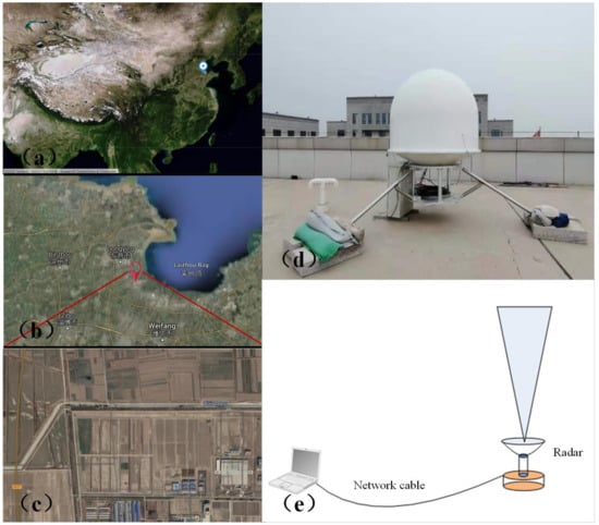
Figure 1.
Schematic of the experimental monitoring test setup for migratory insects: (a) radar site location (Dongying, Shandong, China. Review number: GS(2018)4786). (b) Magnified radar site location. (c) Schematic diagram of the radar observation area. (d) The Ku-band fully polarimetric entomological radar. (e) Vertical observation. (The Chinese in the figure means the name of location).
In this experiment, the vertical observation sampling mode of radar was selected (Figure 1d), and the main parameters of the entomological radar are shown in Table 1.

Table 1.
Main entomological radar parameters.
We took the insect body length as the consideration standard of morphological parameters, and the incident angle as the consideration standard of observation parameters. The specific algorithms come from our team and are introduced as follows.
For the extraction of body length, our team proposed a retrieval method of insect body length based on polarization invariants by using insect data measured in a microwave anechoic chamber. In this method, the Ku-band fully polarimetric entomological radar is used to obtain the target scattering matrix, and the body length of the target is retrieved using the eigenvalue of the scattering matrix and an empirical equation [7].
The fitting empirical equation of body length is a third-order polynomial, as follows:
where is the determinant value of the Graves power matrix, and is the body length in mm.
For the extraction of orientation, based on the research on the RCS characteristics of insect body axis orientation polarization, our team proposed a body axis orientation retrieval method based on fully polarimetric radar [27,28]. For insects with a small body length, compared with radar wavelength, when the polarization direction of the electromagnetic wave is parallel to the insect body axis, the RCS of the insects reaches the maximum.
The direction of maximum RCS of insects is shown as follows:
where S is the scattering matrix of the measurement target, is one of the eigenvalues of the target Graves power matrix, is the Graves power matrix, and are the four components of the Graves power matrix. means that the researcher should take the real part of the complex number.
We further processed the raw data of body length and orientation, as explained in a later section.
2.2. Ideal Insect RCS Simulation
The main methods to obtain the RCS of an individual insect are experimental measurement and simulation. However, to assess field sample insects with different morphological parameters and measure their scattering characteristics is impractical. In this section, we used FEKO (version: 2017.1), an electromagnetic simulation software, to simulate the RCS of an individual insect and establish a database of the scattering characteristics of insects.
We used the ellipsoid spinal cord model for electromagnetic scattering simulation [6]. The density of the spinal cord medium is 1.038 g/cm3 and the relative dielectric constant, at 2.8 GHz, is . Previously, our team measured 183 insects from 22 species in a darkroom experiment, and the results showed that the average value of insect axial ratio was 3.8599 [29]. In order to further simplify the simulation modeling, the body axis ratio of the ellipsoidal insect model was set as 4:1. The schematic diagram of the ellipsoid model is shown in Figure 2.
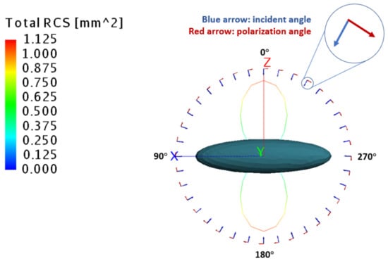
Figure 2.
Simulation modeling and results for an individual insect.
The simulation was set to a monostatic condition. Since this model was used to analyze the linear relationship between RCS and weather radar reflectivity, the incident wave frequency was set to 2.8 GHz in the weather radar band [30]. The polarization angle is shown in Figure 2. What is noteworthy is that when the incident angle is perpendicular to the long axis of the ellipsoid (0° in Figure 2), the polarization angle is parallel to the long axis. Due to the symmetry of the ellipsoid target, the RCS values of any plane around the long axis of the ellipsoid are correspondingly equal. Therefore, we set the incident angle to rotate once clockwise around the xz axis (Figure 2); the step length is 10°, and the z axis is 0°. Figure 2 shows the simulation results of an ellipsoid model with a body length of 15 mm. The blue arrow in Figure 2 is the incident angle, and the red arrow is the polarization angle. Only one excitation source was set for each simulation, and 36 simulations with different incident angles were carried out. Figure 2 shows the incidence angle, polarization angle and radar backscatter cross-sections for 36 simulations around the xz axis. The colored curve is composed of the backscattering cross-sections corresponding to 36 simulations, and its color corresponds to the color bar in the upper left corner.
According to the simulation results in Figure 2, the individual insect is obviously affected by the incident angle and is symmetrically distributed. The RCS of an individual insect reaches the minimum at the head (tail), the maximum at the abdomen (back), and the RCS ratio between the abdomen (back) and the head (tail) reaches 2.5 times. This shows that different incident angles will lead to great differences in RCS.
We performed the electromagnetic simulation described above on individual insects with a body length ranging from 2 mm–26 mm (1 mm step length), then established a database. The ratio of the maximum target size to the wavelength of this database is within the range of 0.019–0.243. However, as there is only qualitative analysis without strict limits for the division into Rayleigh region, resonance region and optical region of ellipsoid targets, we conduct analysis through the data in Figure 3.
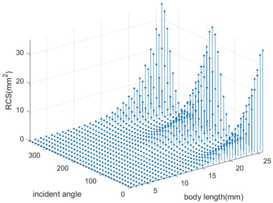
Figure 3.
Schematic diagram of RCS database of individual insects.
According to the results of Figure 3, in terms of body length, the RCS of individual insects increases exponentially as the body length increases. In terms of incident angle, 0°, 180° and 360° in the figure represent an incident from the angle of the abdomen (back), while 90° and 270° represent an incident from the direction of the head (tail). According to the results, it is found that the insect RCS fluctuates as a cosine with incident angle and reaches the maximum value in the direction of the abdomen (back), and the minimum value in the direction of the head (tail).
3. Methods
The accurate establishment of the average RCS model for insects is the premise of density retrieval according to the radar echo intensity. In this section, we mainly describe how to obtain the average RCS, considering morphological and observation parameters. First, we introduce the scattering characteristics of individual insects and the basic principle of density retrieval. Second, we extract the body length and orientation distribution. Finally, we establish an insect-equivalent RCS model, based on the joint probability distribution model of “body length–incident angle”.
3.1. Scattering Characteristics of Individual Insects
The scattering characteristics of individual insects are determined by insect morphology and the insect dielectric constant. The complexity of its structure and components leads to the complexity of RCS calculation. Therefore, simplified models are generally used to study the scattering characteristics of individual insects. For general species of migratory insects, the ellipsoid equivalent model of spinal cord medium can be used to establish their scattering characteristics [17]. For weather radar and other long-range observation radars, the working wavelength of an insect is small. The RCS can be calculated using the Rayleigh scattering function as follows [31]:
where is the wave number, is wavelength; is relative permittivity; is a complex relationship derived from the scattered electric field and the incident electric field (more details can be found in [31]); and , respectively, represent the semi-major axis and semi-minor axis of the ellipsoid target; is the angle between the built-in electric field unit vector and the incident wave unit vector.
The schematic diagram of the radar observation ellipsoid target is shown in Figure 4. The built-in electric field is calculated from the incident field, which can be decomposed into (Figure 4) and (Figure 4). Thus, the built-in electric field vector could be expressed as a vector sum, weighted by and . The unit vector of the long axis of the ellipsoid is expressed as:
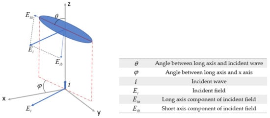
Figure 4.
Schematic diagram of radar observation ellipsoid target.
The unit vector of the short axis of the ellipsoid can be subtracted from the unit vector of the incident electric field and the unit vector of the long axis:
where parameters and are shown in Figure 4.
The above derivation shows that the vector direction of the incident field component is determined by the incident angle, so the built-in electric field is also related to the incident angle.
In summary, according to Equation (4), assuming that the insect medium is the same and the radar parameters are the same, the scattering characteristics of individual insects are closely related to the target’s morphological parameters (body length, body width) and observation parameters (incident angle).
3.2. Retrieval Principle of Insects
The meteorological target is analyzed through the scattering mechanism of the weather radar. The meteorological target (such as cloud and rain) can be assumed to be an isotropic-scattering spherical target with smaller wavelength scale relative to the working wavelength of weather radar. The cumulative RCS per unit volume is called radar reflectivity, expressed as [13]:
In Equation (7), assuming that the cluster targets are uniformly distributed in the radar sampling volume, if is used to represent the average RCS of an individual target in a unit volume, and is the number density of cluster targets, the radar reflectivity can be expressed as:
The radar reflectivity is essentially the total RCS of the particle swarm target per unit volume. Equation (8) can be applied to the density retrieval of insects. Therefore, first, we need to accurately obtain the average RCS of insects.
3.3. Extraction of Parameters Distribution
With respect to the raindrop spectrum, we designed a set of algorithms to process the raw data of body length and orientation. The flow chart of the insect parameter distribution model acquisition algorithm is shown in Figure 5. Firstly, the outliers of body length (2 mm–26 mm) and orientation (−90–90°) retrieval data over 24 h were eliminated. Secondly, the histogram statistics were carried out. Thirdly, the normalized square statistical results were fitted using the “cftool” toolbox in MATLAB (version: 9.9.0.1444674) and we retained the fitting results with a determination coefficient greater than 0.8. Fourthly, the outliers greater than 1 standard deviation of the retained fitting parameters were removed, and finally, the parameters were averaged to extract the insect length distribution and orientation distribution.
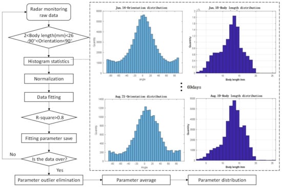
Figure 5.
Flow chart of insect parameter distribution model acquisition algorithm.
In the “Data fitting” step of the flowchart in Figure 5, the fitting basis functions of the body length distribution (Equation (9)) and the orientation distribution (Equation (10)) are as follows:
where is the body length, is the orientation, and are the coefficients to be fitted. The fitting principle of cftool is to find the optimal solution of the coefficient, based on the “basis” function.
For the orientation distribution, we need to consider the following two points:
- Different from body-length distribution, the orientation of insects can vary during the migration process. Therefore, we can only find the distribution rule of insects on both sides of the orientation corresponding to the maximum distribution value (OMDV, in Equation (10)) through curve fitting, but the OMDV cannot be regarded as a fixed value. For example, Figure 6 shows the two orientation probability distribution models of OMDV at 90° and 180°. The shape factors of the two Gaussian distributions are the same, except for the fact that the OMDV is in different positions. Therefore, OMDV is a variable in the model.
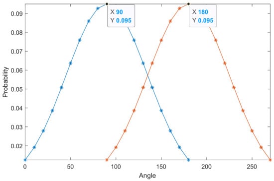 Figure 6. Comparison of orientation distribution of different OMDV. The blue curve represents an orientation distribution of OMDV at 90° and the red curve represents an orientation distribution of OMDV at 180°.
 - The incident angle of an individual insect is determined by the radar-transmitting wave angle and the insect orientation. When the radar-transmitting wave parameters are fixed, the change of the target incident angle is only related to the orientation. Thus, we can convert the orientation to the incident angle using Equation (11). The geometric relationship is shown in Figure 7. Then, the OMDV can be converted to the incident angle corresponding to the maximum distribution value (IAMDV).
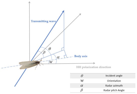 Figure 7. The geometric relationship between orientation and incident angle.
3.4. Parametric Equivalent RCS Model
According to Equation (8), the total RCS can be expressed as:
where is the total RCS of insects; ΔV is the detection volume, is the RCS of an individual insect; is the insect quantity, and is the average RCS of insects.
In order to consider the influence of the morphological and observation parameters proposed in Equation (4), we introduced the body length and incident angle in Section 3.3 into Equation (12).
We established an insect-equivalent RCS model to calculate the average RCS. Equation (12) can be rewritten as follows:
where is the RCS of an individual insect, is its incident angle and is its insect body length, is the incident angle, and is the insect body length.
The establishment process of the insect-equivalent RCS model is shown in Figure 8.
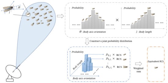
Figure 8.
Schematic diagram of the insect-equivalent RCS model.
The body length and incident angle distributions are continuous functions. However, since it is impractical to extract continuous parameters in actual modeling, the discretization and normalization of the continuous equation are indispensable. The probability distribution model of body length and incident angle are as follows:
It is assumed that the body length normalization vector is expressed as and the incident angle normalization vector is expressed as :
where is the probability that the incident angle of insects is m and is the probability that the body length of insects is .
In order to fuse the normalized distribution characteristics of body length and incident angle, a joint probability distribution model of “body length–incident angle” was obtained by multiplying the transpose of and :
where represents the probability wherein the incident angle is m and the body length is n.
After obtaining the joint probability distribution model of “body length–incident angle”, we need to obtain the RCS values of individual insects at various incident angles and body lengths through electromagnetic simulation or experimental measurement. Since the body length probability distribution is fixed and the incident angle probability distribution changes with IAMDV, we established the equivalent RCS model with incidence angle as an independent variable and average RCS as a dependent variable. Then, the final insect-equivalent RCS model is expressed as:
where and , respectively, represent the probability and the RCS of the individual insect with a corresponding incident angle and body length.
4. Results
4.1. Body Length Probability Distribution Model
The body length distribution results from 69 days of monitoring data are shown as follows:
The body length range of 2–26 mm (1 mm step length) was selected to establish the body length probability distribution model (Equation (14)); the results are shown in Figure 9, where the probability ranges from 0.0002 at 2 mm body length, increasing to a maximum of 0.1334 at 14 mm body length, declining to at 26 mm body length.
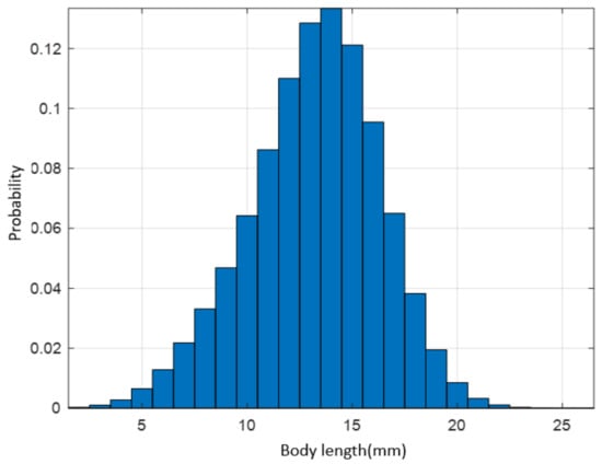
Figure 9.
Probability model of insect body-length distribution.
4.2. Incident Angle Probability Distribution Model
The orientation distribution results from 69 days of monitoring data are shown as follows:
Converting the OMDV into the IAMDV, the incident angle distribution was expressed as:
Taking 9 values on both sides of IAMDV in step 10°, the incident angle probability distribution model with different IAMDV was established.
4.3. Simulation of Insect-Equivalent RCS Model
Putting the body length probability distribution vector and the incident angle probability distribution into Equation (18), we produced the joint probability distribution model. The probability of each point in the joint probability distribution model was weighted with the RCS of the corresponding insect individual, and finally, the insect-equivalent RCS model with different IAMDV is expressed as:
where is the probability of body length l and incident angle in the joint probability distribution model; is the RCS of the body length and incident angle ; is the IAMDV.
Due to the symmetry of the ellipsoid model, this section only calculates the equivalent RCS with IAMDV in the range of 90–180° (Table 2) and extends to 0–360°.
Table 2.
The insect-equivalent RCS with IAMDV in the range of 90–180°.
With the IAMDV as the independent variable and the equivalent RCS as the dependent variable, the insect-equivalent RCS model based on the cosine Equation is as follows:
where is the incident angle corresponding to the maximum distribution value (IAMDV).
The insect-equivalent RCS model is shown in Figure 10.
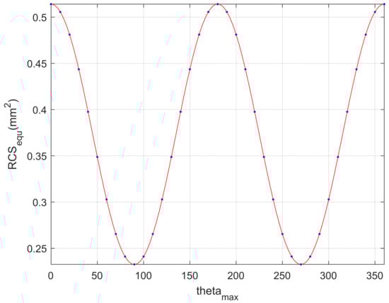
Figure 10.
The insect-equivalent RCS model.
The SSE (sum of the squared errors) of the fitting is only , which proves that the fitting effect is excellent. The maximum value and minimum value of the equivalent RCS were 0.233 mm2 and 0.514 mm2, respectively, with a difference of 0.281 mm2, indicating that the incident angle has some effect on the equivalent RCS of insects.
5. Discussion
We used a self-developed fully polarimetric entomological radar to extract the body length and orientation of raw data and drew them into the insect-equivalent RCS model by establishing probability distribution models. Since the body-length distribution of a given type of insect is relatively fixed, we set the body length probability distribution to a constant. The incident angle of insects can vary during the migration process, so we regard the incident angle as a variable. The dynamic joint probability distribution and the corresponding RCS of individual insects are weighted and summed to obtain the equivalent RCS model. The independent variable and the dependent variable of this model are the incident angle and the average RCS, respectively.
Another way to obtain the average RCS is through the joint observation of weather radar and entomological (bird) radar [12]. Firstly, the reflectivity is obtained by weather radar, then the quantity is obtained by entomological (bird) radar, and finally, the average RCS is obtained according to Equation (8). Compared with this method, our method adds body length and orientation distribution parameters and reduces the systematic error caused by two kinds of radar measurement. Theoretically, our method improves the calculation accuracy of average RCS. Since research on the attitude angles of migratory insects is rare, the model assumed the body axes of the insects are in the horizontal plane. With the development of fine-scale entomological radar monitoring techniques, the model still needs to be improved in the future.
Subsequently, since we currently have no way to achieve full coverage of entomological radars in various regions, we obtained an equivalent RCS model that conforms to the characteristics of the local migrating insects through long-term observation, which ensures the feasibility of the model in practical application. The insect-equivalent RCS model can be combined with weather radar data, which may explain the “dumbbell-like” phenomenon [22] of the weather radar data graph and can compensate for the inaccuracy of weather radar density retrieval. This work will be significant in the development of weather radar insect detection and quantification.
6. Conclusions
To address the problem that morphological parameters and observation parameters are not considered in the current average RCS model for insects, this paper established an insect-equivalent RCS model based on the joint probability distribution of “body length and incident angle”. We used a Ku-band fully polarimetric entomological radar to retrieve the 69-day monitoring data from 14 June 2021 to 21 August 2021 in Dongying, Shandong Province, to extract the parameters of insects and simulate the equivalent RCS model, and finally calculated the typical equivalent RCS model, consistent with the local migration characteristics of insects. The maximum and minimum values of the equivalent RCS in the model are 0.233 mm2 and 0.514 mm2, respectively, indicating that the variation of the insect morphological and observation parameters assuredly causes the fluctuation of insect-equivalent RCS. Therefore, the anisotropy of insect scattering characteristics should be considered when using weather radar for the quantitative estimation of insects. Our results lay a data foundation for the quantitative analysis of insects by weather radar.
Author Contributions
Methodology, R.W., X.K. and K.C.; software, X.K.; validation X.K. and K.C.; resources, K.C.; writing—original draft preparation, X.K.; retrieval of entomological radar data, W.L.; writing—review and editing, R.W., X.K., K.C., H.M., S.W., Z.S., W.L., Y.L. and C.H. All authors have read and agreed to the published version of the manuscript.
Funding
This research was funded by the National Natural Science Foundation of China under Grant No. 31727901, 62001021, and the Major Scientific and Technological Innovation Project under Grant No. 2020CXGC010802.
Conflicts of Interest
The authors declare no conflict of interest.
References
- Holland, R.A.; Wikelski, M.; Wilcove, D.S. How and why do insects migrate? Science 2006, 313, 794–796. [Google Scholar] [CrossRef] [Green Version]
- Satterfield, D.A.; Sillett, T.S.; Chapman, J.W.; Altizer, S.; Marra, P.P. Seasonal insect migrations: Massive, influential, and overlooked. Front. Ecol. Environ. 2020, 18, 335–344. [Google Scholar] [CrossRef]
- Melnikov, V.M.; Istok, M.J.; Westbrook, J.K. Asymmetric Radar Echo Patterns from Insects. J. Atmos. Ocean. Technol. 2015, 32, 659–674. [Google Scholar] [CrossRef]
- Jiang, Y.; Liu, J.; Zeng, J. Using vertical-pointing searchlight-traps to monitor population dynamics of the armyworm Mythimna separate(Walker) in China. Chin. J. Appl. Entomol. 2016, 53, 191–199. [Google Scholar]
- Bridge, E.S.; Thorup, K.; Bowlin, M.S.; Chilson, P.B.; Diehl, R.H.; Fleron, R.W.; Hartl, P.; Kays, R.; Kelly, J.F.; Robinson, W.D.; et al. Technology on the Move: Recent and Forthcoming Innovations for Tracking Migratory Birds. Bioscience 2011, 61, 689–698. [Google Scholar] [CrossRef] [Green Version]
- Wang, R.; Hu, C.; Liu, C.J.; Long, T.; Kong, S.Y.; Lang, T.J.; Gould, P.J.L.; Lim, J.; Wu, K.M. Migratory Insect Multifrequency Radar Cross Sections for Morphological Parameter Estimation. IEEE Trans. Geosci. Remote Sens. 2019, 57, 3450–3461. [Google Scholar] [CrossRef]
- Hu, C.; Li, W.D.; Wang, R.; Long, T.; Liu, C.J.; Drake, V.A. Insect Biological Parameter Estimation Based on the Invariant Target Parameters of the Scattering Matrix. IEEE Trans. Geosci. Remote Sens. 2019, 57, 6212–6225. [Google Scholar] [CrossRef]
- Gauthreaux, S.A., Jr. Weather Radar Quantification of Bird Migration. Bioscience 1970, 20, 17–19. [Google Scholar] [CrossRef]
- Cui, K.; Hu, C.; Wang, R.; Sui, Y.; Mao, H.F.; Li, H.Y. Deep-learning-based extraction of the animal migration patterns from weather radar images. Sci. China-Inf. Sci. 2020, 63, 140304. [Google Scholar] [CrossRef] [Green Version]
- Hu, C.; Cui, K.; Wang, R.; Long, T.; Ma, S.Q.; Wu, K.M. A Retrieval Method of Vertical Profiles of Reflectivity for Migratory Animals Using Weather Radar. IEEE Trans. Geosci. Remote Sens. 2020, 58, 1030–1040. [Google Scholar] [CrossRef]
- Gauthreaux, S.A.; Belser, C.G. Displays of bird movements on the WSR-88D: Patterns and quantification. Weather Forecast. 1998, 13, 453–464. [Google Scholar] [CrossRef]
- Diehl, R.H.; Larkin, R.P.; Black, J.E. Radar observations of bird migration over the Great Lakes. Auk 2003, 120, 278–290. [Google Scholar] [CrossRef]
- Chilson, P.B.; Frick, W.F.; Stepanian, P.M.; Shipley, J.R.; Kunz, T.H.; Kelly, J.F. Estimating animal densities in the aerosphere using weather radar: To Z or not to Z? Ecosphere 2012, 3, 1–19. [Google Scholar] [CrossRef]
- Hajovsky, R.; Deam, A.; LaGrone, A. Propagation, Radar reflections from insects in the lower atmosphere. IEEE Trans. Antennas Propag. 1966, 14, 224–227. [Google Scholar] [CrossRef]
- Aldhous, A.C. An Investigation of the Polarisation Dependence of Insect Radar cross Sections at Constant Aspect. Ph.D. Thesis, Cranfield University, Bedford, UK, 1989. [Google Scholar]
- Vaughn, C.R. Birds and insects as radar targets—A review. Proc. IEEE 1985, 73, 205–227. [Google Scholar] [CrossRef]
- Murton, R.K.; Wright, E.N. The Problems of Birds as Pests: Proceedings of a Symposium Held at the Royal Geographical Society, London, on 28 and 29 September 1967; Elsevier: New York, NY, USA, 2013; pp. 53–86. [Google Scholar]
- Mirkovic, D.; Stepanian, P.M.; Wainwright, C.E.; Reynolds, D.R.; Menz, M.H.M. Characterizing animal anatomy and internal composition for electromagnetic modelling in radar entomology. Remote Sens. Ecol. Conserv. 2019, 5, 169–179. [Google Scholar] [CrossRef]
- Rui, W.; Weidong, L.; Cheng, H.; Muyang, L.; Huafeng, M. Insect Biological Parameters Estimation Method and Field Quantitative Experiment Verification for Fully Polarimetric Entomological Radar. J. Signal Processing 2021, 37, 199–208. [Google Scholar] [CrossRef]
- Townes, H. A light-weight Malaise trap. Entomol. News 1972, 83, 239–247. [Google Scholar]
- Macaulay, E.D.M.; Tatchell, G.M.; Taylor, L.R. The rothamsted insect survey 12-metre suction trap. Bull. Entomol. Res. 1988, 78, 121–129. [Google Scholar] [CrossRef]
- Drake, V.A.; Reynolds, D.R. Radar Entomology: Observing Insect Flight and Migration; Cabi: Wallingford, UK, 2012. [Google Scholar]
- Hu, C.; Li, W.D.; Wang, R.; Long, T.; Drake, V.A. Discrimination of Parallel and Perpendicular Insects Based on Relative Phase of Scattering Matrix Eigenvalues. IEEE Trans. Geosci. Remote Sens. 2020, 58, 3927–3940. [Google Scholar] [CrossRef]
- Teng, Y.; Rui, W.; Muyang, L.; Cheng, H. Research on the Design and Calibration of Wideband Fully Polarized Vertical Insect Radar. J. Signal Processing 2021, 37, 222–233. [Google Scholar] [CrossRef]
- Stepanian, P.M.; Entrekin, S.A.; Wainwright, C.E.; Mirkovic, D.; Tank, J.L.; Kelly, J.F. Declines in an abundant aquatic insect, the burrowing mayfly, across major North American waterways. Proc. Natl. Acad. Sci. USA 2020, 117, 2987–2992. [Google Scholar] [CrossRef] [PubMed]
- Marshall, J. The distribution of raindrops with size. J. Atmos. Sci. 1948, 5, 165–166. [Google Scholar] [CrossRef]
- Hu, C.; Li, W.; Wang, R.; Liu, C.; Zhang, T.; Li, W. Accurate Insect Orientation Extraction Based on Polarization Scattering Matrix Estimation. IEEE Geosci. Remote Sens. Lett. 2017, 14, 1755–1759. [Google Scholar] [CrossRef]
- Muyang, L.; Rui, W.; Teng, Y.; Cheng, H. Influence of Channel Imbalance on Insect Orientation Estimation in Fully Polarimetric Radar. J. Signal Processing 2021, 37, 177–185. [Google Scholar] [CrossRef]
- Kong, S.Y.; Hu, C.; Wang, R.; Zhang, F.; Wang, L.J.; Long, T.; Wu, K.M. Insect Multifrequency Polarimetric Radar Cross Section: Experimental Results and Analysis. IEEE Trans. Geosci. Remote Sens. 2021, 59, 6573–6585. [Google Scholar] [CrossRef]
- Doviak, R.J.; Zrnic, D.S.; Sirmans, D.S. Doppler weather radar. Proc. IEEE 1979, 67, 1522–1553. [Google Scholar] [CrossRef]
- Ishimaru, A. Wave Propagation and Scattering in Random Media; Academic Press: New York, NY, USA, 1978; Volume 1, pp. 407–460. [Google Scholar]
Publisher’s Note: MDPI stays neutral with regard to jurisdictional claims in published maps and institutional affiliations. |
© 2022 by the authors. Licensee MDPI, Basel, Switzerland. This article is an open access article distributed under the terms and conditions of the Creative Commons Attribution (CC BY) license (https://creativecommons.org/licenses/by/4.0/).