Hyperspectral Image Restoration via Spatial-Spectral Residual Total Variation Regularized Low-Rank Tensor Decomposition

Abstract

To eliminate the mixed noise in hyperspectral images (HSIs), three-dimensional total variation (3DTV) regularization has been proven as an efficient tool. However, 3DTV regularization is prone to losing image details in restoration. To resolve this issue, we proposed a novel TV, named spatial domain spectral residual total variation (SSRTV). Considering that there is much residual texture information in spectral variation image, SSRTV first calculates the difference between the pixel values of adjacent bands and then calculates a 2DTV for the residual image. Experimental results demonstrated that the SSRTV regularization term is powerful at changing the structures of noises in an original HSI, thus allowing low-rank techniques to get rid of mixed noises more efficiently without treating them as low-rank features. The global low-rankness and spatial–spectral correlation of HSI is exploited by low-rank Tucker decomposition (LRTD). Moreover, it was demonstrated that the l_2,1 norm is more effective to deal with sparse noise, especially the sample-specific noise such as stripes or deadlines. The augmented Lagrange multiplier (ALM) algorithm was adopted to solve the proposed model. Finally, experimental results with simulated and real data illustrated the validity of the proposed method. The proposed method outperformed state-of-the-art TV-regularized low-rank matrix/tensor decomposition methods in terms of quantitative metrics and visual inspection.

1. Introduction

Hyperspectral imagery (HSI) is composed of numerous narrow spectral bands typically in the range of 400 nm to 2500 nm. Due to its rich spectral information, it can better reflect the reflectance information of ground objects; therefore, it has been widely used in precise agriculture, mineral detection, environment monitoring, urban planning, and so on [1]. Unfortunately, because of facility restrictions, atmospheric conditions, and other unknown factors during the collection process [2], HSI of a real scene is degraded by various noises, such as gaussian noise, impulse noise, stripe, and deadlines. The existence of noise not only reduces visual quality but also limits the processing accuracy in subsequent applications, e.g., unmixing [3], classification [4,5], and target detection [6]. Consequently, restoration of HSI is a critical preprocessing step for effective applications.

A large number of restoration techniques has hitherto been developed for HSI. Filtering-based methods are commonly used because of simplicity [7,8]. However, most of these methods are effective only for a particular noise using a specific filter; the restoration performance is limited for mixed noise. Another popular approach is statistical-based methods [9] usually with the assumption that the noise obeys some probability distribution. In recent years, optimization-based HSI restoration methods have emerged; these methods consider HSI denoising as an optimization problem consisting of regularization and data-fidelity terms. The regularization term helps to exploit prior knowledge about the underlying properties of HSI and noise; therefore, an accurate description of the regularization is prerequisite to good results under ill-posed conditions.

In optimization-based methods, an HSI can be restored by the one dimensional (1D) vector method [10], two dimensional (2D) matrix method [11], or 3 dimensional (3D) tensor method [12,13,14]. In these methods, the HSI is treated as vectors, grayscale matrices, or three-order tensors, respectively. Even though the 1D and 2D methods are always faster, the restoration results are unsatisfactory because they ignore the inherited spectral and spatial correlation of a HSI. To address this issue, various methods to incorporate the prior knowledge of such correlations have been proposed. For instance, a wavelet shrinkage method applied in both spatial and spectral domains was proposed in [15]. Zhao et al. [16] proposed a sparse representation method to jointly utilize the spatial-spectral information of HSI. Considering the differences between spectral noise and spatial information, Yuan et al. [17] proposed a spectral-spatial adaptive total variation model. With the advent of tensor technology, which conveniently deals with the spectral and spatial domain of a HSI simultaneously, increasingly more studies are devoted to tensor-based restoration methods.

A typical HSI has low rank properties. It was claimed in [12] that HSI $\mathcal{X}$ Xhas a specific correlation in both spatial dimensions by observing the obvious decaying trends of the singular value changes of unfolding matrices X₍₁₎ and X₍₂₎, which also indicate that they are low-rank matrices. From the linear mixture point, HSI shows strong spectral correlation, and the mode-3 unfolding matrix X₍₃₎ is a low-rank matrix. As the collected HSIs from real scenes are inevitably contaminated by various noise, they could destroy the low-rank property. Based on the low rank assumption, a low-rank matrix recovery (LRMR) model was proposed in [2] to remove the mixed noise, where an HSI was decomposed into a low-rank part and a sparse part to represent a clean HSI and sparse noises, respectively. Even LRMR can remove Gaussian and sparse noise simultaneously; this method considers only the local similarity within patches. Subsequently, numerous non-convex norms have been proposed to formulate the low-rank property instead of the nuclear norm, for example, γ-norm [18] and weighted Schatten p-norm [19,20]. However, there are three weaknesses with these methods. Firstly, these methods need to reshape the original 3D HSI into a 2D matrix, which will destroy the spectral correlation. Secondly, computational cost is high because one has to compute the matrix singular value decomposition (SVD) in each of the iterations in optimization. Thirdly, the low rank property exists in both spectral and spatial domains [12], but these methods consider the low rank property in the spatial domain and spectral domain separately. Consequently, to utilize the global low-rank property and spatial–spectral correlation of HSI, methods based on the low-rank tensor decomposition (LRTD) have been proposed for HSI restoration [12,13,14]. One major challenge is local, structured sparse noise such as stripes or deadlines. Since these noises are regarded as the low rank component, the low-rank constraint will fail to remove them.

In addition to the low rank property of HSI, it also has a piecewise smooth structure as a natural image in the spatial domain, which can be exploited by total variation (TV) regularization methods [21,22,23,24,25]. For example, He et al. [21] combined band-by-band TV (BTV) regularization with low-rank matrix factorization (LRMF) to improve restoration performance. While BTV is useful to characterize spatial piecewise smoothness, it does not consider spectral correlation of HSI.

To overcome spatial over-smoothing of TV methods, many methods incorporate spectral correlation. For example, Yuan et al. [17] introduced a spectral-spatial adaptive hyperspectral TV (SSAHTV), which realized the band and spatial adaptive denoising process automatically. Zheng et al. [22] extended it to a band group-wise version. Similar approaches that explicitly evaluate spectral correlation in addition to spatial piecewise-smoothness include the spatial-spectral TV (SSTV) [23], anisotropic SSTV (ASSTV) [24], and Cross Total Variation (CrTV) [25]. In the design of SSTV and ASSTV, spatial correlation is interpreted as spectral piecewise smoothness and is evaluated by the l₁ norm of local differences along the spectral direction, resulting in computationally efficient optimization. Specifically, to evaluate spatial and spectral piecewise smoothness simultaneously, SSTV focuses on local spatial-spectral differences. However, as this method ignores direct local spatial differences, the restored HSI tends to have artifacts, especially in highly noisy scenarios. While ASSTV handles both local spatial and spectral differences directly in parallel, it often produces spectrally over-smoothed images because it strongly suppresses the l₁ norm of direct spectral differences for HSI. SSAHTV can adaptively estimate the denoising strength according to different spatial properties and different noise intensity in bands.

The other method is three-dimensional spectral-spatial TV (3DSSTV, or 3DTV for brief) and its variants. The 3DTV [26] is defined as

$$\Vert \mathcal{X}{\Vert }_{3\mathrm{DTV}} = w_1{D}_h\mathcal{X} + w_2{D}_v\mathcal{X} + w_3{D}_p\mathcal{X} = \sum _{i,j,k}(w_1\left|x_{i + 1,j,k} - x_{i,j,k}\right| + w_2\left|x_{i,j + 1,k} - x_{i,j,k}\right| + w_3\left|x_{i,j,k + 1} - x_{i,j,k}\right|$$

(1)

The $D_h$, $D_v,$ and $D_p$ are difference operators along the horizontal, vertical, and spectral directions, respectively. The $w_1,w_{2,} \mathrm{and} w_3$ are the weights corresponding with $D_h$, $D_v,$ and $D_p$. The 3DTV has been combined with LRTD [26] and t-SVD [27] to remove mixed noise in HSI. In general, the combination of a low-rank tensor and 3DTV regularization restoration model achieves better results. It is noteworthy that the 3DTV is different from the aforementioned SSTV. The SSTV is defined as the TV of the unfolding matrix of HSI, as such SSTV indeed belongs to 2DTV.

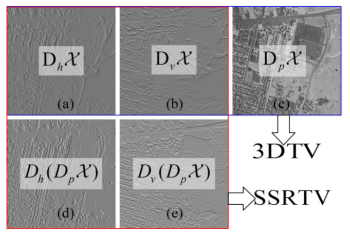
Although the 3DTV defined in Equation (1) considered both spatial and spectral smoothness, there still is one problem. The difference images in 3DTV, which are calculated by $D_h$, $D_v,$ and $D_p,$ are presented in Figure 1. Figure 1a–c shows the images of $D_h\mathcal{X},$ $D_v\mathcal{X},$ and $D_p\mathcal{X}$ for real Urban dataset $\mathcal{X}$, respectively. The 3DTV along the spectrum considers that the content of the adjacent bands is close to each other, and the variation of $D_p\mathcal{X}$ is sparse. However, it can be observed from Figure 1c that the variation along spectrum $D_p\mathcal{X}$ still leaves lots of details. 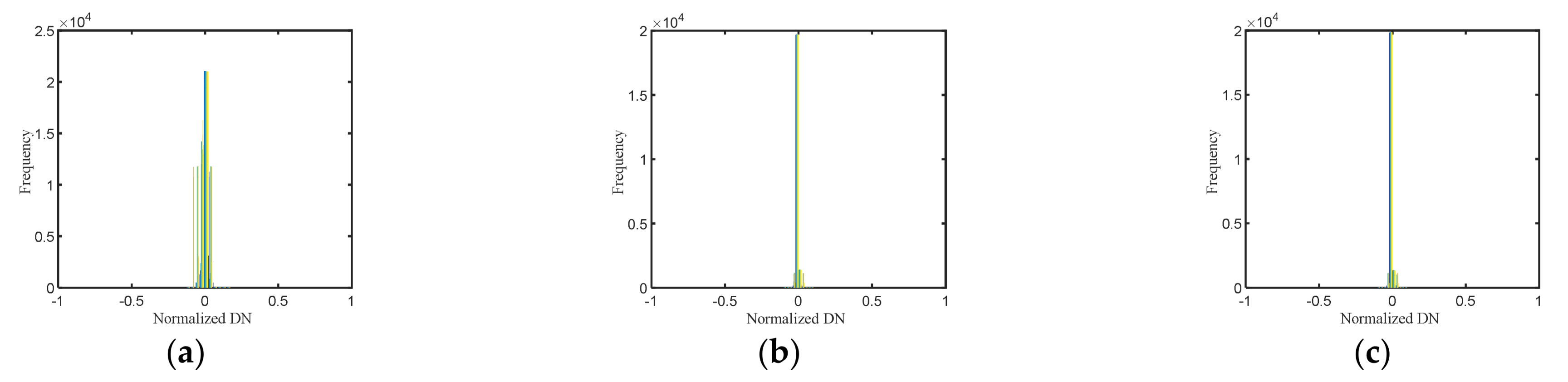Therefore, the real value of 3DTV in HSI is relatively large (see Figure 2a).

Figure 2 shows the histograms of $D_p\mathcal{X}$, $D_h\left(D_p\mathcal{X}\right),$ and $D_v\left(D_p\mathcal{X}\right)$, respectively. The more detailed the image is, the larger the real 3DTV norm is. Therefore, if 3DTV is minimized as a constraint condition for HSI restoration, there is a great possibility of loss of image details, with a sub-optimal effect. To overcome the aforementioned drawbacks and effectively utilize the prior knowledge on HSI, we proposed a Spatial-Spectral Residual Total Variation (SSRTV) regularization technique for HSI restoration. The SSRTV is designed to evaluate two types of local differences: direct local spatial differences ($D_h\mathcal{X},D_v\mathcal{X}$) and local spatial-spectral differences ($D_h\left(D_p\mathcal{X}\right),D_v\left(D_p\mathcal{X}\right)$) in a unified manner with a balancing weight. This design resolves the drawbacks of the existing TV regularization techniques mentioned above. Generally speaking, $D_h\left(D_p\mathcal{X}\right) \mathrm{and} D_v\left(D_p\mathcal{X}\right)$ are calculated with the 2DTV on the residual image $D_p\mathcal{X}$. Then, the local correlation within the bands is actually considered, which would promote a much stronger sparsity than $D_p\mathcal{X}$ (see Figure 1d,e, and the corresponding histograms in Figure 2b,c). $D_h\left(D_p\mathcal{X}\right) \mathrm{and} D_v\left(D_p\mathcal{X}\right)$ are expressed as:

$$D_h\left(D_p\mathcal{X}\right) = \Vert D_h{\mathcal{M}}_1\Vert = {\sum }_{i,j,k}\left|{\mathcal{M}}_{i + 1,j,k} - {\mathcal{M}}_{i,j,k}\right|$$

(2)

$$D_v\left(D_p\mathcal{X}\right) = \Vert D_v{\mathcal{M}}_1\Vert = {\sum }_{i,j,k}\left|{\mathcal{M}}_{i,j + 1,k} - {\mathcal{M}}_{i,j,k}\right|$$

(3)

where ${\mathcal{M}}_{i,j,k} = {\mathcal{X}}_{i,j,k + 1} - {\mathcal{X}}_{i,j,k}$ is the difference of band k + 1 and k for pixel at spatial location (i, j).

Although the SSRTV defined here looks similar to the Hybrid Spatio-Spectral Total Variation (HSSTV) in reference [28], there are essential differences between them. In fact, the $D_h\left(D_{p}u\right) \mathrm{and} D_v\left(D_{p}u\right)$ in HSSTV mean $D_h\left(D_p{\mathcal{X}}_{\left(1\right)}\right)$ and $D_v\left(D_p{\mathcal{X}}_{\left(2\right)}\right)$, where ${\mathcal{X}}_{\left(1\right)}$ and ${\mathcal{X}}_{\left(2\right)}$ are the unfolding matrices along the horizontal (mode-1) and vertical (mode-2).

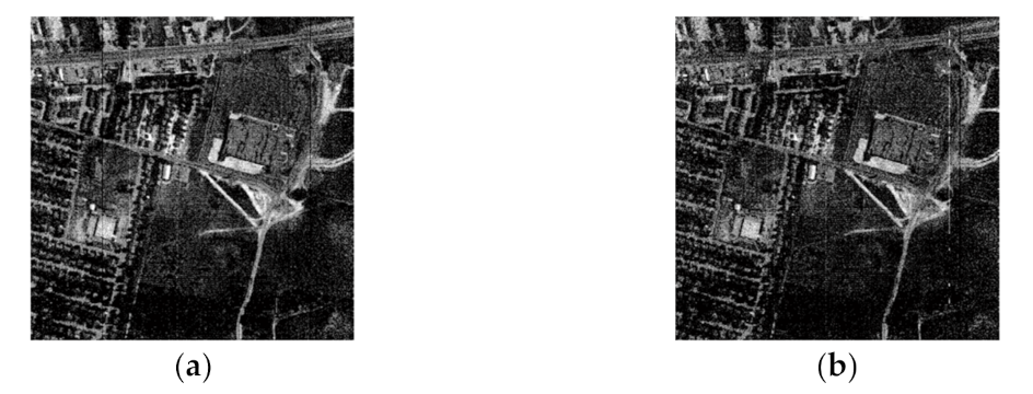
In addition, the deadlines, stripes, and impulse noises were assumed to be sparse [2]. Among these sparse noises, the stripes or deadlines showed a certain directional characteristic, as shown in Figure 3. When the sparse noises at the same place occurred in most of the bands, they were treated as the low-rank component and could not be removed by the low-rank-based method [21].

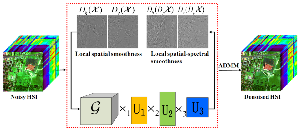
To remove the mixed noise in the HSI, we designed a spatial domain spectral Residual Total Variation regularization approach combined with LRTD (LRTDSSRTV). Figure 4 presents the flowchart of our method.

It was found that SSRTV is totally different from the previous TV regularization in [25,29]. Our proposed HSI restoration method combined SSRTV with the low-rank Tucker decomposition framework. To summarize, the major contributions of this paper are as follows.

(1)

We designed a Spatial-Spectral Residual Total Variation (SSRTV) to better capture both the direct spatial and spatial-spectral piecewise smoothness of HSI. This can overcome disadvantages of previous TV methods, that is, the low-rank regularization fails to remove the structured sparse noise.

(2)

The SSRTV was incorporated into the LRTD model to separate the underlying clean HSI from its degraded version with mixed noise. LRTD was adopted to preserve the global spatial and spectral correlation of HSI and restore the clean low-rank HSI.

(3)

The classical higher-order orthogonal iteration (HOOI) algorithm [30] was adopted to achieve the Tucker decomposition efficiently, without bringing an extra computational burden. By using alternating direction method of multipliers (ADMM), our method was split into several simpler sub-problems. Compared with the methods based on low-rank matrix/tensor decomposition, the experimental results with the simulations and real data validated the proposed method.

The remaining contents are organized as follows. In Section 2, we present notations for tensor operations. Our restoration model and its optimization are described in Section 3. The effectiveness of the proposed method was verified by the experiments of simulated data sets and real remote sensing data sets, shown in Section 4. Finally, the conclusions are drawn, and outlook is presented in Section 5.

2. Notations and Preliminaries

In tensor algebra, a tensor is a multi-linear mapping defined on a Cartesian product of some vector spaces and some dual spaces. The order of a tensor is defined as the number of its dimensions or modes. For example, scalar, vector, and matrix are zero-order tensor, one-order tensor, and two-order tensor, respectively. The corresponding representations are a lowercase letter, lowercase boldface letter, and capitalized boldface letter. For instance, the $x$, x, and X are scalar, vector, and matrix, respectively. An N-order (N ≥ 3) tensor is denoted by a capitalized calligraphic letter, i.e., $\mathcal{X}$. The HSI data cube is a three-order tensor. For an N-dimensional real valued tensor $\mathcal{X}\in {ℝ}^{I_1 \times I_2 \times \cdots \times I_N}$, we used $x_{i_1,i_2,\cdots ,i_N}$ to represent its element at location ($i_1,i_2,\cdots ,i_N$), and its Nth dimension is also called Nth mode. By fixing all the indices but the nth index, we obtained the mode-n fibers. By arranging all the mode-n fibers as columns, we obtained a matrix denoted by ${\mathcal{X}}_{\left(n\right)}$ or $X_{\left(n\right)}\in {ℝ}^{I_n \times {\prod }_{k = 1,k\ne n}^N{I}_k}$. This process is also called the mode-n matrixing of $\mathcal{X}$ or unfolding along mode-n. The multi-linear rank of $\mathcal{X}$ is an array ($r_1,r_2,\cdots ,r_N$) and r_i = rank (X_(i)), I = 1, 2, …, N.

The inner product of two tensors $\mathcal{X}$ and $\mathcal{Y}$ was calculated by $\langle \mathcal{X},\mathcal{Y}\rangle = {\sum }_{i_1,i_2,\cdots ,i_N}{x}_{1,i_2,\cdots ,i_N} \cdot y_{i_1,i_2,\cdots ,i_N}$. The l₁-norm of tensor $\mathcal{X}$ was calculated as ${\Vert \mathcal{X}\Vert }_1 = {\sum }_{i_1,i_2,\cdots ,i_N}\left|x_{i_1,i_2,\cdots ,i_N}\right|$. The l_2,1-norm of matrix X was calculated as ${\Vert X\Vert }_{2,1} = {\sum }_{j = 1}^J\sqrt{{\sum }_{i = 1}^I\left|x_{i,j}^2\right|}$. The tensor-matrix product by mode-n was defined as ${\left(\mathcal{Y}{\times }_n\mathbf{U}\right)}_{i_1\cdots i_{n - 1},i_{n + 1},\cdots ,i_N}={\sum }_{i_n}{x}_{i_1,i_2,\cdots ,i_N} \cdot u_{j,i_n}$. For more information of tensor algebra, please refer to [30].

3. Proposed Model

3.1. Observation Model with Mixed Noise

From the mathematics view, the HSI may be contaminated by additive and multiplicative noise. In this work, we considered mainly the additive noise, including Gaussian, impulse, stripe, and deadlines [2]. The multiplicative noise can be transformed into additive noise with the Logarithmic transformation [31]. The Gaussian noise was caused by poor lighting and/or high temperature of the imaging sensors, meanwhile the sparse noise can be introduced by mechanical imperfection of push-broom sensors, e.g., deadlines and stripes. Following the most popular HSI restoration model [12,32], the HSI degraded by mixed noise was formulated in the following:

$$\mathcal{Y} = \mathcal{X} + \mathcal{S} + \mathcal{N}$$

(4)

In model (4), $\mathcal{Y},\mathcal{X},\mathcal{S},\mathcal{N}\in {ℝ}^{m \times n \times b}$ are all three-order tensors, and they denote the observed degraded HSI, latent clean HSI, the sparse noise (e.g., impulse, stripe, and deadlines), and Gaussian noise, respectively. The size m × n × b indicates that the HSI has b spectral bands and the resolution of each band grayscale image is m × n. The existence of noise will hinder the understanding of HSI. The purpose of restoration focuses on removing the noise from an observed noisy image $\mathcal{Y}$ and restoring a latent image $\mathcal{X}$. This pre-processing can improve the awareness level and further processing of his.

Recovering $\mathcal{X}$ from $\mathcal{Y}$ with Equation (4) is a difficult ill-condition problem [12,32]. To tackle this problem, a typical practice is to exploit the priors of all involved variables. The general mixed noise restoration model for HSIs can be formulated as

$$\underset{\mathcal{X},\mathcal{S}}{argmin}R\left(\mathcal{X}\right) + \rho R\left(\mathcal{S}\right) + \gamma R\left(\mathcal{N}\right) \mathrm{s}.\mathrm{t}. \mathcal{Y} = \mathcal{X} + \mathcal{S} + \mathcal{N}$$

(5)

where $R\left(\mathcal{X}\right)$, $R\left(\mathcal{S}\right)$, and $R\left(\mathcal{N}\right)$ are the regularization terms to model the priori with respect to a clean HSI $\mathcal{X}$, sparse noise $\mathcal{S},$ and Gaussian noise $\mathcal{N}$, respectively. Parameters ρ and γ are the positive regularization parameters that maintain the trade-off between the three regularization terms. Since the Gaussian noise $\mathcal{N}$ is typically depicted by l₂ norm and $\mathcal{N} = \mathcal{Y} - \mathcal{X} - \mathcal{S}$, the Equation (5) can be transformed to its equivalent form

$$\underset{\mathcal{X},\mathcal{S}}{argmin}R\left(\mathcal{X}\right) + \rho R\left(\mathcal{S}\right) \mathrm{s}.\mathrm{t}. \Vert \mathcal{Y} - \mathcal{X} - {\mathcal{S}\Vert }_F^2\le {\sigma }^2$$

(6)

Here, σ² is a parameter related to the density of Gaussian noise.

3.2. Directional Structure Sparse Priori of S

For non-Gaussian noise such as deadlines, stripes, and impulse noises, they are generally considered as having a sparse property [2], and the sparseness property for the sparse noise $\mathcal{S}$ is characterized by l₁ norm ${\Vert \mathcal{S}\Vert }_1$ [12,32,33,34]. The directional characteristic of stripes and deadlines show that they have structure sparse property, as shown in Figure 3. While the l₁ norm cannot depict this structure sparse property, the l_2,1-norm is a sparsity-inducing norm defined as the l₁-norm of the columns of matrix. It has the advantage of being rotation invariant when compared with the traditional l₁ norm [35]. It has been demonstrated in [36] that the l_2,1-norm is more robust with respect to outliers, especially for structure sparse noise, such as stripes and deadlines [35]. In this paper, we extended the l_2,1 norm of a matrix to impose sparsity, that is ${\Vert \mathcal{X}\Vert }_{2,1} = {\sum }_{k = 1}^b{\sum }_{j = 1}^n\sqrt{{\sum }_{i = 1}^m\left|x_{i,j,k}^2\right|}$. Therefore, mathematically, the objective function can be written as follows:

$$\underset{\mathcal{X},\mathcal{S}}{min}R\left(\mathcal{X}\right) + \rho {\Vert \mathcal{S}\Vert }_{2,1},\mathrm{s}.\mathrm{t}. \Vert \mathcal{Y} - \mathcal{X} - {\mathcal{S}\Vert }_F^2\le {\sigma }^2$$

(7)

3.3. Low-Rank Priori of HSI

In light of the linear mixture model [37], HSI shows strong spectral correlation. Based on this assumption, the mode-3 unfolding matrix ${\mathcal{X}}_{\left(3\right)}$ is a low-rank matrix. Besides, by observing the notable descent of the singular value curves of mode-1 unfolding matrix ${\mathcal{X}}_{\left(1\right)}$ and mode-2 unfolding matrix ${\mathcal{X}}_{\left(2\right)}$, it was reported in [12] that HSI also showed strong spatial correlation. To jointly consider the correlations of HSI in both spatial and spectral domains, the low-rank Tucker decomposition was utilized to aggregate the factor matrix of a clean HSI $\mathcal{X}$: $R_1\left(\mathcal{X}\right) = \Vert \mathcal{X} - \mathcal{G}{\times }_1{\mathbf{U}}_1{\times }_2{\mathbf{U}}_2{\times }_3{\mathbf{U}}_3\Vert {}_F^2$, where factorization matrices ${\mathbf{U}}_1\in {ℝ}^{m \times r_1}$(with rank r₁), ${\mathbf{U}}_2\in {ℝ}^{n \times r_2}$(with rank r₂), and ${\mathbf{U}}_3\in {ℝ}^{b \times r_3}$(with rank r₃) are orthogonal in both spatial modes and spectral modes, respectively, and $\mathcal{G}\in {ℝ}^{r_1 \times r_2 \times r_3}$ is called the core tensor.

Restoring HSI by combining LRTD with 3DTV regularization, considering global spatial-spectral correlation and spatial-spectral smoothness, the restored HSI achieved satisfactory results [12]. Nevertheless, there are still some problems. The 3DTV-regularized-based model explores the sparse priori of the spatial-spectral difference images. However, the variation along the spectral domain still left lots of details. Therefore, the real value of 3DTV in HSI was relatively large. To effectively utilize a priori knowledge for HSI restoration, we proposed a new TV regularization technique to simultaneously evaluate the direct local spatial differences and local spatial-spectral differences, which is expected to resolve the drawbacks of the existing TV regularization techniques.

3.4. SSRTV Regularization

Our new regularization technique for HSI restoration is named SSRTV. It is defined as

$$\mathrm{SSRTV}\left(\mathcal{X}\right) = w_1{D}_h\mathcal{X} + w_2{D}_v\mathcal{X} + w_3\left[D_h\left(D_p\mathcal{X}\right) + D_v\left(D_p\mathcal{X}\right)\right]$$

(8)

The $D_h$, $D_v,$ and $D_p$ are the same difference operators as in Equation (1). The $D_h{D}_p\left(·\right)$ and $D_v{D}_p\left(·\right)$ are defined in Equations (2) and (3). They are local spatial-spectral differences of $\mathcal{X}$, as shown in Figure 1 (box with dotted, red lines). The weights w₁, w_2, and w₃ are used to balance the importance of spatial-spectral piecewise smoothness and direct spatial piecewise smoothness.

Different from $D_p\mathcal{X}$ in 3DTV, to obtain $D_h\left(D_p\mathcal{X}\right) and D_v\left(D_p\mathcal{X}\right)$, the difference of pixels in the same spatial position of adjacent bands is calculated first. Then, 2DTV is calculated for the residual image $D_p\mathcal{X}$. Due to the similarity between adjacent bands, the two-dimensional gradient of the residual image is more sparse than the two-dimensional gradient of the original image most likely, which leads to the minimum real norm value in the noise-free HSI. On the other hand, due to the disorder of noise, the obtained norm value of a noisy HSI is bound to be much larger than that of the noise-free HSI. Therefore, if the regularization term is minimized, the image details can be maintained with high probability while removing noise.

3.5. Model Proposal and Optimization

Traditional 3DTV only considers the spatial-spectral piecewise smoothness. As a result, the similar sparse noise in adjacent bands would be treated as a low-rank component and failed to be removed. Based on this observation, we put forward a spatial domain spectral residual total variation-regularized low-rank tensor decomposition (LRTDSSRTV) method. The low-rank tensor Tucker decomposition is used to keep the global spatial-spectral correlation. Except for the direct spatial difference $D_h\left(\mathcal{X}\right) \mathrm{and} D_v\left(\mathcal{X}\right)$, the spatial difference of spectral difference $D_h\left(D_p\mathcal{X}\right) \mathrm{and} D_v\left(D_p\mathcal{X}\right)$ in SSRTV regularization can change the structure of sparse noise. The restoration model combining SSRTV with LRTD is given as follows:

$$\underset{\mathcal{X},\mathcal{S}}{argmin}\rho {\Vert \mathcal{S}\Vert }_{2,1} + w_1{D}_h\left(\mathcal{X}\right) + w_2{D}_v\left(\mathcal{X}\right) + w_3\left[D_h\left(D_p\mathcal{X}\right) + D_v\left(D_p\mathcal{X}\right)\right]$$

$$\mathrm{s}.\mathrm{t}. \mathcal{X} = \mathcal{G}{\times }_1{\mathit{U}}_1{\times }_2{\mathit{U}}_2{\times }_3{\mathit{U}}_3,{\mathit{U}}_k^T{\mathit{U}}_k = \mathit{I},\Vert \mathcal{Y} - \mathcal{X} - {\mathcal{S}\Vert }_F^2\le {\sigma }^2$$

(9)

In Equation (9), we fully exploit the priors of the clean HSI component and noise component. The LRTD is utilized to maintain the spatial-spectral correlation of HSI, while the SSRTV is used to exploit local spatial-spectral smoothness of HSI. The tensor formulation with l_2,1-norm is utilized to separate the sparse noise, and the Gaussian noise is eliminated by the Frobenius norm.

Due to the non-differential property of the model (9), an alternate updating scheme was presented. We introduced the ADMM [38] to optimize it. By introducing auxiliary variables $\mathcal{Z}$ and D_k (k = 1, 2, 3, 4, 5), a new objective function can be written as,

$$\underset{\mathcal{X},\mathcal{S},D_1,D_2,D_3,D_4,D_5}{min}\rho {\Vert \mathcal{S}\Vert }_{2,1} + \tau \{w_1\Vert D_1\Vert {}_1 + w_2\Vert D_2\Vert {}_1 + w_3\left[\Vert D_4\Vert {}_1 + \Vert D_5\Vert {}_1\right]$$

$$\mathrm{s}.\mathrm{t}. \mathcal{X} = \mathcal{G}{\times }_1{\mathit{U}}_1{\times }_2{\mathit{U}}_2{\times }_3{\mathit{U}}_3,\mathcal{X} = \mathcal{Z},D_1 = D_h\mathcal{Z},D_2 = D_v\mathcal{Z},D_3 = D_p\mathcal{Z},D_4 = D_h{D}_3,D_5 = D_v{D}_3$$

(10)

All the constraints except $\mathcal{X} = \mathcal{G}{\times }_1{\mathit{U}}_1{\times }_2{\mathit{U}}_2{\times }_3{\mathit{U}}_3$ were taken into account, and the Augmented Lagrangian form of (10) is given by

$$\begin{gathered} \mathcal{L}\left(\mathcal{X},\mathcal{S},\mathcal{G},{\mathbf{U}}_i,\mathcal{Q},{\Lambda }_j\right) = \rho {\Vert \mathcal{S}\Vert }_{2,1} + \tau \left\{w_1\Vert D_1\Vert {}_1 + w_2\Vert D_2\Vert {}_1 + w_3\left[\Vert D_4\Vert {}_1 + \Vert D_5\Vert {}_1\right]\right\} \\ +\frac{\mu }{2}(\Vert D_1 - D_h\mathcal{Z} + {\Lambda }_1\Vert {}_F^2 + \Vert D_2 - D_v\mathcal{Z} + {\Lambda }_2\Vert {}_F^2 + \Vert D_3 - D_p\mathcal{Z} + {\Lambda }_3\Vert {}_F^2 + \end{gathered}$$

$$\Vert D_4 - D_h{D}_3 + {\Lambda }_4\Vert {}_F^2 + \Vert D_5 - D_v{D}_3 + {\Lambda }_5\Vert {}_F^2 + \Vert \mathcal{Y} - \mathcal{X} - \mathcal{S} + {\Lambda }_6\Vert {}_F^2 + \Vert \mathcal{X} - \mathcal{Z} + {\Lambda }_7\Vert {}_F^2)$$

(11)

where ${\mathit{U}}_i^T{\mathit{U}}_i = \mathit{I}$ (i = 1; 2; 3), $\mu$ is the penalty parameter, and Λ_j (j = 1; 2; 3; 4; 5; 6; 7) is the Lagrange multipliers related to corresponding variables.

Problem (11) is a multi-objective optimization problem. All variables involved in (11) cannot be jointly optimized. By using ADMM, variables in (11) can be alternatively optimized with an individual, solvable subproblem while keeping the others fixed. Following this arrangement, we decomposed (11) into six independent subproblems and their corresponding solutions are presented.

(1) Update $\mathcal{G}$, ${\mathit{U}}_i,$ and $\mathcal{X}$. All the terms related to $\mathcal{X}$ were extracted from (11), and we obtained

$$\underset{\mathcal{X}}{argmin}\frac{\mu }{2}(\Vert \mathcal{Y} - \mathcal{X} - \mathcal{S} + {\Lambda }_6\Vert {}_F^2 + \Vert \mathcal{X} - \mathcal{Z} + {\Lambda }_7\Vert {}_F^2)$$

(12)

Combining with the constraints $\mathcal{X} = \mathcal{G}{\times }_1{\mathit{U}}_1{\times }_2{\mathit{U}}_2{\times }_3{\mathit{U}}_3$ and ${\mathit{U}}_i^T{\mathit{U}}_i = \mathit{I}$ (i = 1; 2; 3), the problem (12) can be transformed into its equivalent form:

$$\underset{\mathcal{G},{\mathit{U}}_j}{argmin}\mu (\Vert \mathcal{G}{\times }_1{\mathit{U}}_1{\times }_2{\mathit{U}}_2{\times }_3{\mathit{U}}_3 - {\frac{\left(\mathcal{Y} - \mathcal{S} + \mathcal{Z} + {\Lambda }_6 - {\Lambda }_7\right)}{2}\Vert }_F^2)$$

(13)

By using the higher-order orthogonal iteration (HOOI) algorithm [30], it was easy to get the nuclear tensor $\mathcal{G}$ and factor matrix ${\mathit{U}}_j$. Then, $\mathcal{X}$ can be updated by $\mathcal{X} = \mathcal{G}{\times }_1{\mathit{U}}_1{\times }_2{\mathit{U}}_2{\times }_3{\mathit{U}}_3$.

(2) Update $\mathcal{S}$: All the terms related to $\mathcal{S}$ are given by

$$\underset{\mathcal{S}}{argmin}\rho {\Vert \mathcal{S}\Vert }_{2,1} + \frac{\mu }{2}\Vert \mathcal{Y} - \mathcal{X} - \mathcal{S} + {\Lambda }_6\Vert {}_F^2$$

(14)

Let $\mathcal{Y} - \mathcal{X} + {\Lambda }_6 = \mathcal{C}$, following [36]; then, $\mathcal{S}$ can be updated by the following rule

$$\mathcal{S}\left(:,j,k\right)=\left\{\begin{array}{cc}\frac{\Vert \mathcal{C}\left(:,j,k\right)\Vert - \frac{\rho }{\mu }}{\Vert \mathcal{C}\left(:,j,k\right)\Vert }\Vert \mathcal{C}\left(:,j,k\right)\Vert ,& \mathit{if}\frac{\rho }{\mu } < \Vert \mathcal{C}\left(:,j,k\right)\Vert \\ 0,& \mathrm{otherwise}\end{array}\right.$$

(3) Update D₁:

$$\underset{D_1}{argmin}\tau w_1\Vert D_1\Vert {}_1 + \frac{\mu }{2}\Vert D_1 - D_h\mathcal{Z} + {\Lambda }_1\Vert {}_F^2$$

(15)

This is a soft-thresholding problem. The close-form solution is

$$D_1 = \mathcal{T}\left(D_h\mathcal{Z} - {\Lambda }_1,\frac{\tau w_1}{\mu }\right)$$

(16)

where $\mathcal{T}\left(a,b\right) = \mathrm{sign}\left(a\right) \cdot \mathit{max}(\left|a\right| - b,0)$.

Similarly, the D₂, D_4, and D₅ can be updated by

$$D_2 = \mathcal{T}\left(D_h\mathcal{Z} - {\Lambda }_2,\frac{\tau w_2}{\mu }\right)$$

(17)

$$D_4 = \mathcal{T}\left(D_h{D}_3 - {\Lambda }_4,\frac{\tau w_3}{\mu }\right)$$

(18)

$$D_5 = \mathcal{T}\left(D_v{D}_3 - {\Lambda }_5,\frac{\tau w_3}{\mu }\right)$$

(19)

(4) Update D₃:

$$\underset{D_3}{argmin}\frac{\mu }{2}\left(\Vert D_3 - D_p\mathcal{Z} + {\Lambda }_3\Vert {}_F^2 + \Vert D_4 - D_h{D}_3 + {\Lambda }_4\Vert {}_F^2 + \Vert D_5 - D_v{D}_3 + {\Lambda }_5\Vert {}_F^2\right)$$

(20)

This is a quadratic optimization problem, and it is equivalent to solving the following linear system is:

$$\left(\mathbf{1} + D_h^T{D}_h + D_v^T{D}_v\right)D_3 = D_p\mathcal{Z} - {\Lambda }_3 + D_h^T\left(D_4 + {\Lambda }_4\right) + D_v^T\left(D_5 + {\Lambda }_5\right)$$

(21)

By using the fast Fourier transform (FFT), the closed form solution of (21) is

$$D_3 = {\mathcal{F}}^{ - 1}\left\{\frac{\mathcal{F}\left[D_p\mathcal{Z} - {\Lambda }_3 + D_h^T\left(D_4 + {\Lambda }_4\right) + D_v^T\left(D_5 + {\Lambda }_5\right)\right]}{\mathbf{1} + \mathcal{F}{(D_h)}^{\ast }\mathcal{F}\left(D_h\right) + \mathcal{F}{(D_v)}^{\ast }\mathcal{F}\left(D_v\right)}\right\}$$

(22)

where $\mathcal{F}\left(·\right)$ and ${\mathcal{F}}^{ - 1}\left(·\right)$ represent the 3D FFT and the inverse 3D FFT, respectively. The symbols T and * respectively represent the operators of transpose and complex conjugate.

(5) Update $\mathcal{Z}$:

$$\underset{\mathcal{Z}}{argmin}\frac{\mu }{2}\left(\Vert D_1 - D_h\mathcal{Z} + {\Lambda }_1\Vert {}_F^2 + \Vert D_2 - D_v\mathcal{Z} + {\Lambda }_2\Vert {}_F^2 + \Vert D_3 - D_p\mathcal{Z} + {\Lambda }_3\Vert {}_F^2 + \Vert \mathcal{X} - \mathcal{Z} + {\Lambda }_7\Vert {}_F^2\right)$$

(23)

This is also a quadratic optimization problem, and the corresponding linear system is

$$\left(\mathbf{1} + D_h^T{D}_h + D_v^T{D}_v + D_p^T{D}_p\right)\mathcal{Z} = \left(\mathcal{X} + {\Lambda }_7\right) + D_h^T\left(D_1 + {\Lambda }_1\right) + D_v^T\left(D_2 + {\Lambda }_2\right) + D_p^T\left(D_3 + {\Lambda }_3\right)$$

(24)

It is easy to get the closed form solution in (25) by 3D FFT,

$$\mathcal{Z} = {\mathcal{F}}^{-1}\left\{\frac{\mathcal{F}\left(\mathcal{X} + {\Lambda }_7 + \mathit{\Delta }\right)}{\left(1 + D\right)}\right\}$$

(25)

where $D = \mathcal{F}{(D_h)}^{\ast }\mathcal{F}\left(D_h\right) + \mathcal{F}{(D_v)}^{\ast }\mathcal{F}\left(D_v\right) + \mathcal{F}{(D_p)}^{\ast }\mathcal{F}\left(D_p\right)$ and $\mathit{\Delta } = D_h^T\left(D_1 + {\Lambda }_1\right) + D_v^T\left(D_2 + {\Lambda }_2\right) + D_p^T\left(D_3 + {\Lambda }_3\right)$.

(6) Update Multipliers: On the basis of the augmented Lagrange multiplier algorithm [39], the Lagrange multipliers Λ_i (i = 1, 2, 3, 4, 5, 6, 7) can be updated as follows:

$${\Lambda }_1 = {\Lambda }_1 + \mu \left(D_1 - D_h\mathcal{Z}\right)$$

(26)

$${\Lambda }_2 = {\Lambda }_2 + \mu \left(D_2 - D_v\mathcal{Z}\right)$$

(27)

$${\Lambda }_3 = {\Lambda }_3 + \mu \left(D_3 - D_p\mathcal{Z}\right)$$

(28)

$${\Lambda }_4 = {\Lambda }_4 + \mu \left(D_4 - D_h{D}_3\right)$$

(29)

$${\Lambda }_5 = {\Lambda }_5 + \mu \left(D_5 - D_v{D}_3\right)$$

(30)

$${\Lambda }_6 = {\Lambda }_6 + \mu \left(\mathcal{Y} - \mathcal{X} - \mathcal{S}\right)$$

(31)

$${\Lambda }_7 = {\Lambda }_7 + \mu \left(\mathcal{X} - \mathcal{Z}\right)$$

(32)

The pseudocode in Algorithm 1 summarizes the above optimization process. In the LRTDSSRTV solver, the inputs are the noisy image $\mathcal{Y}$, regularization parameters ρ and τ, the weights w_i s, estimated rank (r₁, r₂, r₃) for Tucker decomposition, the stopping criteria ε, the maximum iteration k_max, μ_max = 10⁶, and η = 1.5. More details and discussions are presented in Section 4.

Algorithm 1: Optimization Process for LRTDSSRTV Solver

Input: Noisy image $\mathcal{Y}$, regularization parameters ρ and τ, the weights wi s, estimated rank (r1, r2, r3) for Tucker decomposition, the stopping criteria ε, the maximum iteration kmax, μmax = 106, and η = 1.5.

1: Initialize: Let $\mathcal{X}$ = $\mathcal{Y}$, Di = 0 (i = 1, 2, 3, 4, 5), Λj = 0 (j = 1, 2, 3, 4, 5, 6, 7), current iteration k = 0, and μmax = 106

2: while not converged do

3: Update $\mathcal{G}$ and ${\mathbf{U}}_i$ via (13) and then $\mathcal{X}=\mathcal{G}{\times }_1{\mathbf{U}}_1{\times }_2{\mathbf{U}}_2{\times }_3{\mathbf{U}}_3$.

4: Compute $\mathcal{S}$ via (14).

5: Update D1, D2, D4, D5 via (16)–(19).

6: Compute D3 via 3D FFT (22).

7: Update $\mathcal{Z}$ via 3D FFT (25)

8: Compute the Lagrange multipliers Λj by (26)–(32).

9: Update the penalty parameter μ = min{ημ, μmax}.

10: Check the convergence condition k < kmax and $\frac{\Vert {\mathcal{X}}^{\left(k + 1\right)} - {\mathcal{X}}^{\left(k\right)}\Vert {}_F^2}{\Vert {\mathcal{X}}^{\left(k\right)}\Vert {}_F^2} \le \epsilon$.

11: end while

Output: The restoration result $\mathcal{X}$.

4. Experimental Results and Analysis

In this section, the simulated and real datasets were adopted to evaluate the proposed LRTDSSRTV solver. To better validate the advantages of the LRTD and SSRTV regularization, we selected five representative advanced methods to compare, including low-rank matrix recovery (LRMR) [2], the combination of low-rank matrix factorization with TV regularization (LRTV) [21], anisotropic spatial-spectral TV regularization with low-rank tensor decomposition (LRTDTV) (http://gr.xjtu.edu.cn/web/dymeng/3, (accessed on 12 June 2021)) [12], the spatial-spectral TV model (SSTV) (https://sites.google.com/view/hkaggarwal/publications (accessed on 12 June 2021)) [23], and Weighted Group Sparsity-Regularized Low-Rank Tensor Decomposition(LRTDGS) (http://www.escience.cn/people/yongchen/index.html (accessed on 12 June 2021)) [32]. LRMR imposes spectral low-rankness in spatial patches. LRTV combines a low-rank constraint of the unfolding matrix with HSI and BTV. LRTDTV jointly considers 3DTV and Tucker decomposition. SSTV applies 1-D total variation on the spectral domain. LRTDGS introduces weighted group sparse regularization to improve the group sparsity of the spatial difference image. According to the authors’ suggestions, we carefully tuned the parameters involved in the compared methods to guarantee optimal results. While for the parameters in our method, a detailed discussion of parameter selection is presented in Section 4. In addition, all the bands of the HSI were normalized within the range of [0, 1] for easy numerical calculation and visualization, and the HSI was transformed to original grayscale level after restoration.

4.1. Experiment with Simulated Data

(1) Experimental Setting: In this section, we evaluated the robustness of a simulated clean Indian Pines’ dataset with synthetic noise. This dataset contained 224 bands; each band was a grayscale image of 145 × 145 pixels. It was widely used in [12,21,40]. This dataset was firstly used in [2], which was generated from the real Indian Pines’ dataset. The reflectance values of all the pixels were mapped to [0; 1] through linear transform.

To simulate complicated noise cases in a real scene, six representative types of noise were added. The rules for adding noise were as follows:

Case 1: A zero-means Gaussian noise. In a real scene, the noise density in each band should be different. Therefore, we added randomly selected noise variances to each band within the range of [0, 0.25].

Case 2: Different intensities of Gaussian noise to each band, as in Case 1. Additionally, we added deadlines from bands 141 to 170. The number of the deadline in each band was randomly selected between 3 and 10, and the deadline’s width was randomly generated from 1 to 3 pixels.

Case 3: Gaussian noise was added in the same way as in case 2. Additionally, the impulse noise was added to all bands and the percentages were randomly selected within the range of [0, 20%].

Case 4: On the basis of case 3, we added stripes to bands 161 to 190; the number of stripes in each band was randomly selected in the range of 10 to 30.

Case 5: The deadline was added in the same way as in case 2, and the stripe noise was added as in case 4. Additionally, the impulse noise was also added, and the percentages were varied from 0 to 50% for each band.

Case 6: All the considered noises were added to simulate the most severe noise situation. Gaussian noise, stripes, and impulse noise were added in the same way as in case 4. Additionally, 30 bands were randomly chosen to add deadlines, and the number of deadline were randomly selected from 3 to 10.

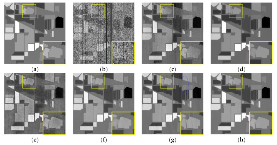
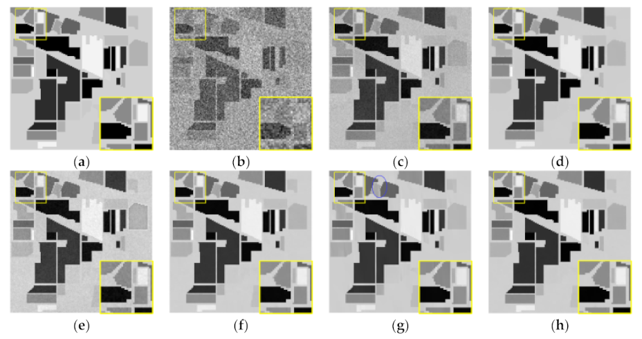
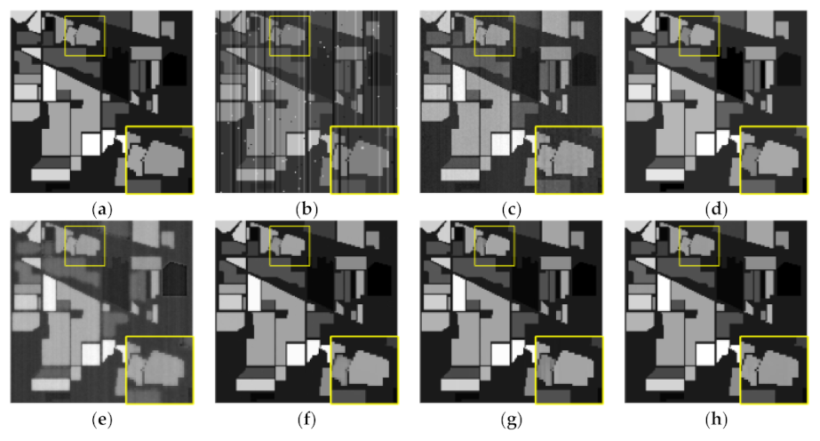
(2) Visual Comparison: One important outcome of restoration is to improve the visual quality. To illustrate, we show three representative cases, 1, 5, and 6, in Figure 5, Figure 6 and Figure 7, respectively, with the restoration results for bands 46, 168, and 162. For better visualization, we provided a zoom with yellow boxes. It can be observed that the denoised result of (c) LRMR and (e) SSTV did not completely eliminate the noise in the presented results (see the zoom boxes). Restoration results of (d) LRTV, (f) LRTDTV, and (g) LRTDGS were satisfactory, completely removing all noises. However, the details of some areas in the image of LRTV and LRTDTV were blurred (see the zoom boxes). Some striped artifacts were observed from the zoom boxes with the result of (g) LRTDGS. Additionally, there was obvious noise in the result of SSTV, as observed in Figure 7e. By contrast, the proposed LRTDSSRTV method can remove all kinds of noises and maintain an image feature and detail with better visual quality than the comparison methods. This is due to the simultaneous consideration of both spatial spectral piecewise smoothness and direct spatial piecewise smoothness in SSRTV.

(3) Quantitative Comparison: Four objective quantitative evaluation indices (QEI) were used to compare the results of all the methods in each simulated experiment, including peak signal-to-noise ratio (PSNR) [dB] index, the structural similarity (SSIM) index [41], erreur relative globale adimensionelle de synthese (ERGAS; relative dimensionless global error in synthesis in English), and the spectral angle mapper (SAM) [42]. For the PSNR and SSIM, we showed the average values (or means) of all the HSI bands, denoted by MPSNR and MSSIM, respectively. The higher values of MPSNR and MSSIM or the lower values of ERGAS and SAM represented better restoration results.

The values of four QEIs of all the methods under the simulated six different noise cases are presented in

Table 1. Quantitative comparison of all comparison methods on the simulated indian pines in six different noise cases.

Noise Case	Evaluation Index	Noise	LRMR	LRTV	SSTV	LRTDTV	LRTDGS	LRTDSSRTV
CASE 1	MPSNR (dB)	20.373	33.265	37.053	32.117	39.957	40.216	41.895
	MSSIM	0.3896	0.8978	0.9834	0.8587	0.9912	0.9939	0.9963
	ERGAS	380.198	48.91	47.303	60.23	24.371	24.306	23.561
	SAM	0.3201	0.0366	0.0403	0.0445	0.0149	0.0149	0.0136
CASE 2	MPSNR (dB)	18.972	33.294	36.268	31.616	38.582	39.456	40.818
	MSSIM	0.3953	0.9073	0.9838	0.8649	0.9888	0.9933	0.9958
	ERGAS	346.025	47.540	46.265	60.061	30.873	25.216	23.529
	SAM	0.2906	0.0364	0.0369	0.0449	0.0217	0.0174	0.0157
CASE 3	MPSNR (dB)	12.782	32.603	36.103	31.002	37.702	39.141	39.891
	MSSIM	0.2183	0.8928	0.9816	0.8472	0.9866	0.9936	0.9921
	ERGAS	500.499	50.092	56.685	63.562	30.005	25.254	24.130
	SAM	0.4001	0.0376	0.0435	0.0473	0.0185	0.0165	0.0173
CASE 4	MPSNR (dB)	12.725	32.423	36.033	30.886	37.3536	38.897	39.963
	MSSIM	0.2167	0.8902	0.9814	0.8432	0.9859	0.9928	0.9934
	ERGAS	502.705	3.227	3.597	4.069	2.094	1.612	1.539
	SAM	0.4014	0.0387	0.0460	0.0482	0.0217	0.0171	0.0166
CASE 5	MPSNR (dB)	11.296	36.425	37.382	37.157	39.465	41.419	44.403
	MSSIM	0.1946	0.9481	0.9804	0.9587	0.9886	0.9938	0.9949
	ERGAS	624.857	39.753	89.326	40.931	40.974	28.466	25.653
	SAM	0.4908	0.0301	0.0638	0.0252	0.0264	0.0120	0.0108
CASE 6	MPSNR (dB)	12.589	32.124	34.739	30.768	37.427	38.102	38.963
	MSSIM	0.2140	0.8889	0.9748	0.8420	0.9855	0.9903	0.9926
	ERGAS	509.281	54.096	72.748	66.103	35.117	30.921	27.102
	SAM	0.4079	0.0414	0.0584	0.0495	0.0246	0.0221	0.0193

. The best values among the comparison methods are highlighted in bold, while the suboptimal values are underlined. By comparison, we can see that the tensor-based methods (LRTDTV, LRTDGS and LRTDSSRTV) by and large performed better than the matrix-based methods. The main reason is that LRTD can capture the global correlation both in spatial and spectral dimensions. In comparison with LRTDTV and LRTDGS, our method shows superiority in all QEIs under almost all cases. The reason is that the 3DTV norm used in LRTDTV calculates and sums the gradient values in three directions at the same time, and the actual norm results are relatively large. Therefore, minimizing 3DTV as a constraint condition for HSI restoration would tend to lose image details during restoration. For the group sparsity used in LRTDGS, it strengthens the spatial constraints while failing to explore the spectral constraint. Our method remedies the deficiency and makes an improvement in all QEIs for the Indian Pines’ dataset.

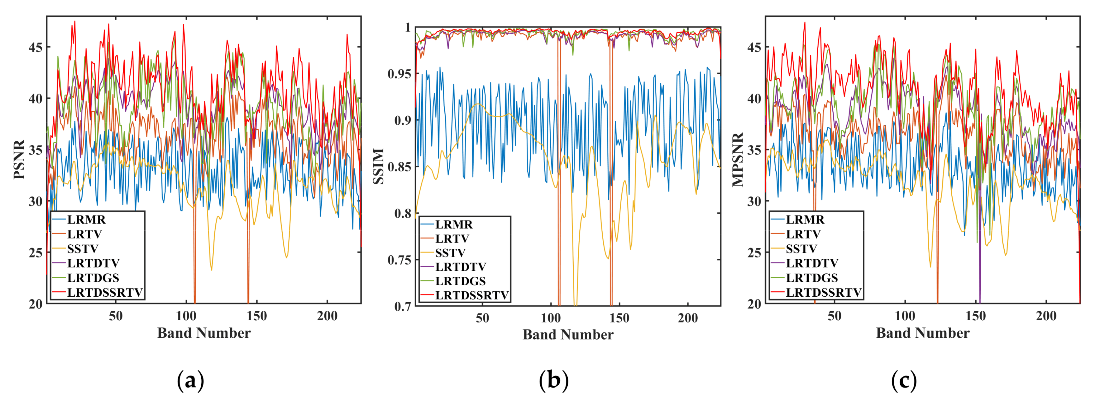
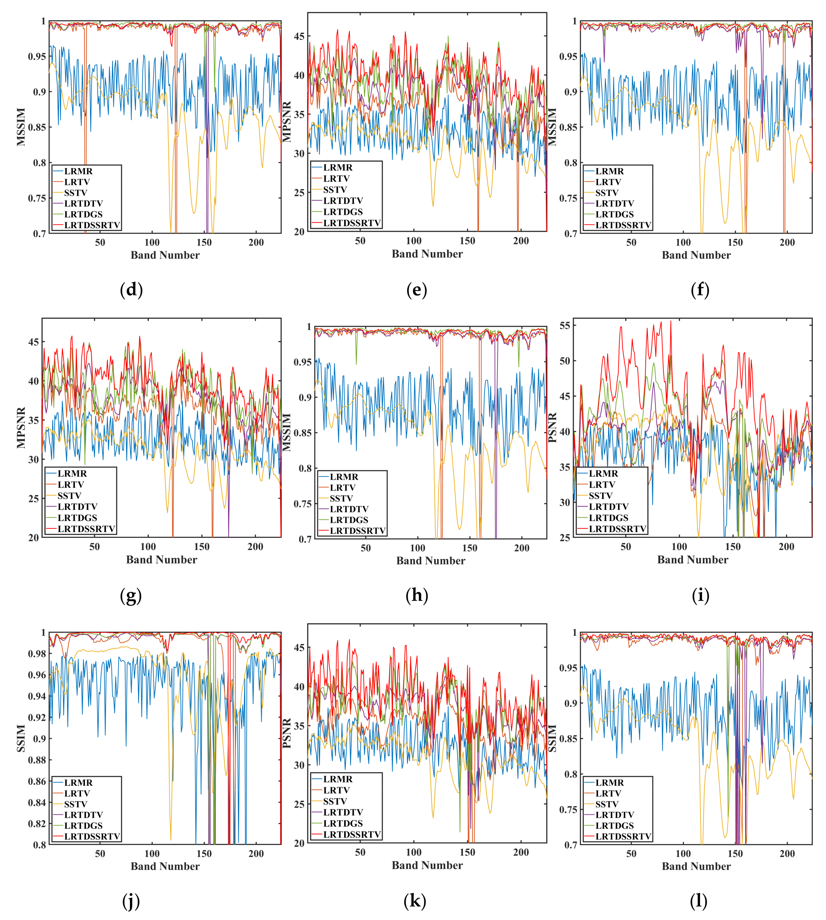
To take a close look at the PSNR and SSIM values of each band. Figure 8 shows the corresponding curves of these two QEIs in six cases. It is observed that the PSNR and SSIM values of LRMR and SSTV were obviously lower than other four methods. Although the PSNR and SSIM values of LRTV were higher than LRMR and SSTV, this indicates that LRTV can get better denoised results in the spatial domain. We can see that the spectral distortion of LRMR is still serious in Table 1. Compared with LRTDTV and LRTDGS, the proposed LRTDSSRTV method achieved much higher SSIM and PSNR values for almost all the bands.

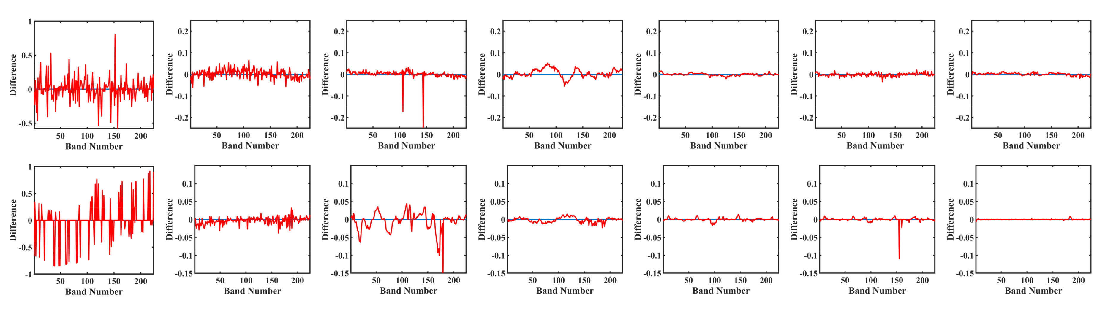
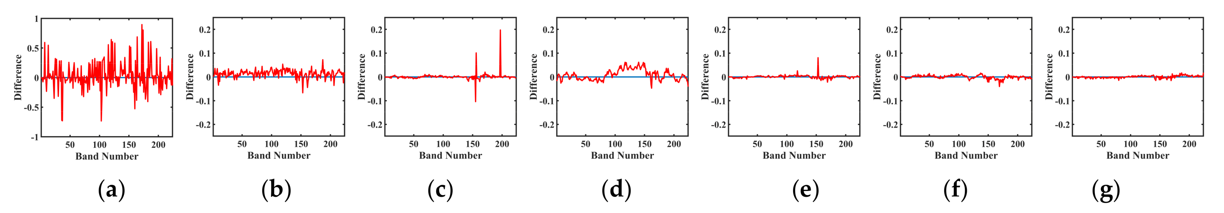
To further illuminate the qualitative comparison in terms of spectral information, the spectral difference between the original spectrums and the restored ones at different locations under cases 1, 5, and 6 are presented in Figure 9. The horizontal axis in Figure 9 denotes band number, while the vertical axis denotes the spectral difference. It can be seen from Figure 9 that the LRTD-based methods (LRTDTV, LRTDGS, and our method) achieved better spectral fidelity than other three methods. This phenomenon indicates that the global LRTD can efficiently preserve the spatial-spectral correlation of HSI. However, compared with LRTDTV and LRTDGS, the spectral differences of our method were the smallest. This result is consistent with the values of the ERGAS index in Table 1.

4.2. Real-World Data Experiments

In this section, we conducted experiments with two real case datasets. One is the Airborne Visible/Infrared Imaging Spectrometer (AVIRIS) Indian Pines’ dataset and the other is the Hyperspectral Digital Imagery Collection Experiment (HYDICE) urban dataset. Before processing, the pixel value was also normalized to [0, 1] band by band.

4.2.1. AVIRIS Indian Pines’ Dataset

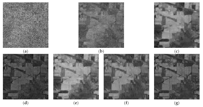
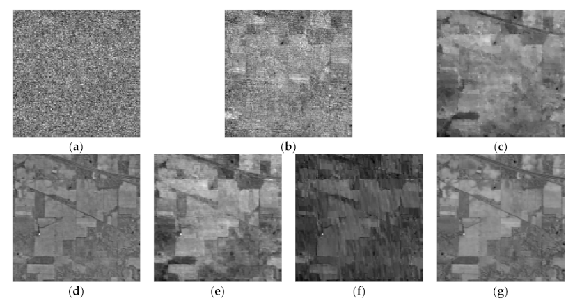
The spatial resolution of this dataset was 145 × 145, and it contained 220 bands. The noises existing in this dataset were mainly Gaussian and impulse noises. For brevity, two typical bands, 104 and 150, were selected to show the restoration results of different methods. Figure 10a and Figure 11a correspond to the original bands 104 and 150, respectively. It was found that these two bands were both severely degraded by mixed noise. Therefore, the useful information was almost completely corrupted. After restoration, there were some noises in the results of LRMR. Even the LRTV could remove the noise, but the edges were over-smoothed. The same situation happened in the results of SSTV, LRTDTV, and LRTDGS. Especially, the details of LRTDGS were blurred seriously, as shown in Figure 11f. Compared with TV regularization methods, our method performed the best in removing noise and preserving edges and local details.

4.2.2. HYDICE Urban Dataset

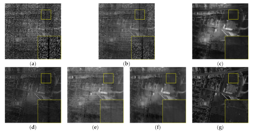
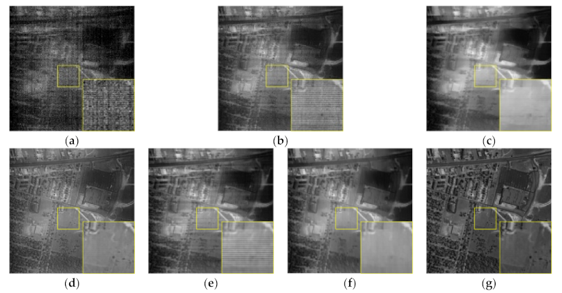
The spatial resolution of this dataset was 307 × 307, and it contained 210 bands. The noise in this dataset was more complicated than in the AVIRIS Indian Pines’ Dataset. Except for the Gaussian noise, deadlines, impulse noise, and stripes, it may also have been degraded by water absorption, atmosphere, and some other unknown noises. For brevity and readability, two representative noise bands were chosen to compare the denoising performance. The original bands, 108 and 208, and their corresponding denoised results are shown in Figure 12, Figure 13 and Figure 14, respectively. Figure 12a and Figure 14a represent the original bands, 108 and 208, respectively. There were mixed noise and bias illumination, which changed the image contrast, in these two bands. Figure 12b–g and Figure 14b–g were the denoised results with different restoration methods. It can be seen from the zoom boxes in Figure 12b–g that there were still a few stripes existing in the results of the methods LRMR, LRTV, SSTV, and LRTDTV. Even though LRTDGS can remove most noise, it resulted in a blurred edge in some regions. It can be seen from Figure 14a that there were obvious deadlines in the original band. All the five compared methods failed to eliminate the deadlines, and LRMR also failed to remove other noises. A benefit of the SSRTV regularization and global LRTD, as shown in Figure 12g and Figure 14g, our method removed not only mixed noises but also bias illumination. By comparison, the LRTV and LRTDTV just considered the $D_h\mathcal{X} \mathrm{and} D_v\mathcal{X}$. Therefore, they could not completely get rid of the bias illumination. Both SSTV and LRTDSSRTV considered the $D_h\left(D_p\mathcal{X}\right),D_v\left(D_p\mathcal{X}\right)$, and the bias illumination was removed, as shown in Figure 12d and Figure 14g, while the visual quality of SSTV was not as good as that of LRTDSSRTV for failing to consider $D_h\mathcal{X} \mathrm{and} D_v\mathcal{X}$ in SSTV.

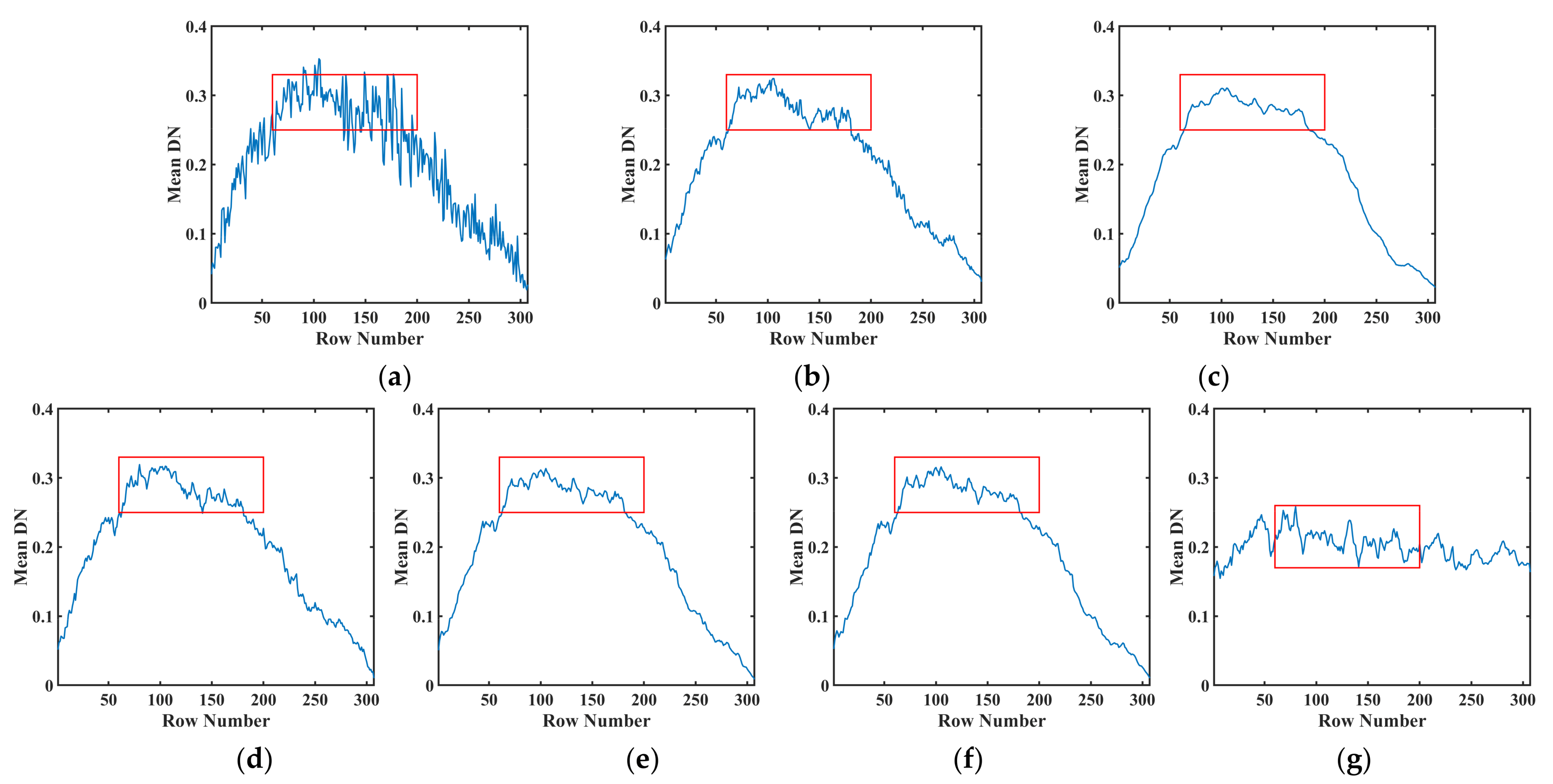
To further compare the restoration results, the mean digital number (MDN) corresponding to Figure 12 and Figure 14 is shown in Figure 13 and Figure 15, respectively. The horizontal axis represents the row number and the vertical axis denotes the MDN of each row. It can be seen from Figure 12a that rapid fluctuations occurred in the curve for the existence of stripes and other noises. It is observed from Figure 13b–g that the fluctuations were reduced by all the methods. As shown in Figure 13b–e, due to the stripes in the image, there were some minor fluctuations in the curve, which is consistent with the restoration results shown in Figure 12b–e. Figure 12f shows the smoothed result of LRTDGS, which can also be confirmed from Figure 13f. By contrast, the proposed method achieved more reasonable mean profile results, as shown in Figure 13g.

4.3. Classification Performance Comparison

To further compare the performance of different denoising methods and the influence of denoising on classification application, real dataset, Indian pines, used in Section 4.2, was selected. The effectiveness of the proposed algorithm and its influence on classification were verified by comparing the classification accuracy with the basic threshold classifier (BTC) [43].

To compare the classification accuracy of different algorithms obtained by the classifier, three common evaluation indicators were used here: (1) Overall Accuracy (OA), that is, the number of correctly classified samples was divided by the number of test samples. OA is obtained by using 10% of the samples of each class for training and the remaining 90% for testing; (2) average accuracy (AA), namely, the average of classification accuracy of all available categories; and © Kappa coefficient (Ka), which is a statistical measure of the consistency between the final classification map and the real classification map. The formula of Kappa is as follows:

$$\mathrm{Kappa} = \frac{N{\sum }_{j = 1}^m{x}_{jj} - {\sum }_{j = 1}^m(x_{j + }{x}_{ + j})}{N^2 - N{\sum }_{j = 1}^m(x_{j + }{x}_{ + j})}$$

(33)

where m is the column number of error matrix, $x_{jj}$ represents the element in the position of column j, and line j in the error matrix. The $x_{j + }$ is the sum of row j in the error matrix. The $x_{ + j}$ is the sum of column j in the error matrix. N is the number of test samples.

The larger the values of Kappa (no unit), OA (given in percentage form), and AA (given in percentage form), the better the classification effect of the algorithm. The Indian pines’ dataset contains 16 classes, and the specific class names can be found on the website http://www.ehu.eus/ccwintco/index.php?title=Hyperspectral_Remote_Sensing_Scenes (accessed on 12 June 2021).

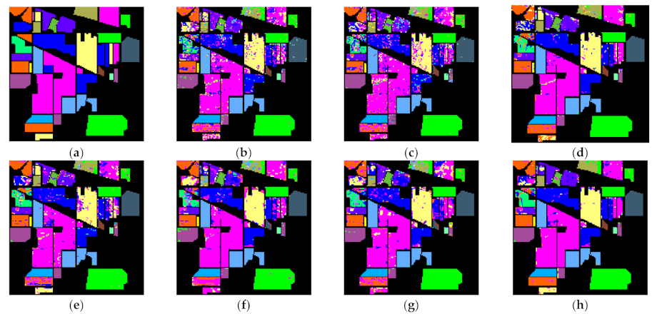
Figure 16b shows the classification map obtained by applying BTC on the original Indian Pines’ data set. Figure 16c–h shows the classification map obtained by applying BTC after denoising on the Indian Pines’ data set using LRMR, LRTV, SSTV, LRTDTV, LRTDGS, and SSRTV. It was observed that BTC was seriously affected by noise on the original data, which made the classification accuracy low. Different denoising methods reduced this effect more or less and improved the classification accuracy. Compared with other algorithms, the proposed algorithm showed a more excellent performance.

Table 2. Classification indexes of Indian pines and the denoised results by different methods.

Index	Original	LRMR	LRTV	SSTV	LRTDTV	LRTDGS	LRTDSSRTV
OA	79.24	81.39	81.99	86.99	86.64	87.08	91.11
AA	78.37	80.97	81.14	86.95	85.58	87.01	90.34
Ka	0.7621	0.7712	0.7731	0.8336	0.7884	0.7944	0.8982

shows the indices by using BTC to classify the original Indian pines’ data and the denoised data. Three indices after denoising by all methods increased more or less. Different denoising results had different degrees of improvement in classification accuracy. For example, the denoising results of the LRMR method still contained a large amount of noise, so the Ka, OA, and AA values only increased by about 2%, 2%, and 0.01%, respectively. The Ka, OA, and AA values of the proposed algorithm increased about 12%, 12%, and 0.13%, respectively. Obviously, the proposed algorithm significantly improved the classification accuracy.

5. Discussion

(1)

Parameters’ selection

In this section, we will address how to determine the parameters in our experiments with systematical analysis. The choosing of parameters was based on the simulated experiment in the Indian pines’ dataset.

In our model, there were two regularization parameters, ρ and τ; one penalty parameter, μ; three weight parameters, w₁, w₂, and w₃; and Tucker rank (r₁, r₂, r₃) among the three HSI modes. For penalty parameter μ, it was first initialized as μ = 10⁻² and updated by μ = min (ημ, μ_max), where η = 1.5 and μ_max = 10⁶. This strategy of determining the variable µ has been widely used in the ALM-based method [12], which can facilitate the convergence of the algorithm.

For the Tucker rank (r₁, r₂, r₃), following the same strategy proposed in [32], we set r₁ and r₂ as 80% of the width and height of each band image, respectively. In our simulated experiments, we set r₃ = 10. In the real data experiments, the r₃ was estimated by HySime [44].

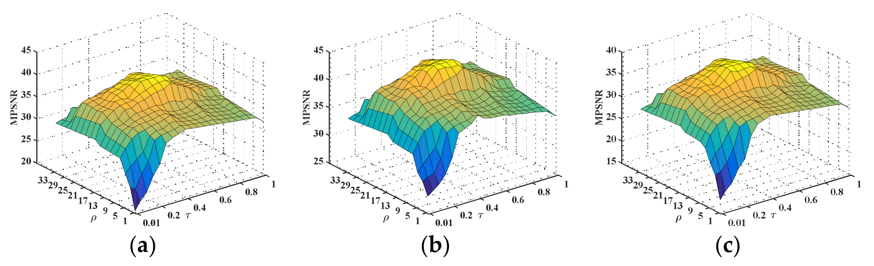
The parameter ρ corresponded to the sparse term. It was set as $\Vert \rho \Vert = \frac{100 \times C}{\sqrt{mn}}$ by default in the following experiments according to [12,32], where m and n were the width and height of each band image of HSI and C was a parameter that needed to be carefully tuned. Therefore, we jointly tuned the parameters ρ and τ. We also chose the simulated cases 1, 5, and 6 to present the sensitivity analyses of these two parameters, and the MPSNR was used as the evaluation index. Figure 17 shows the MPSNR values as ρ varied in the set [1, 3, 5, 7, 9, 11, 13, 15, 17, 19, 21, 23, 25, 27, 29, 31, 33] and τ varied in the set [0.01, 0.05, 0.1, 0.15, 0.2, 0.25, 0.3, 0.35, 0.4, 0.45, 0.5, 0.55, 0.6, 0.65, 0.7, 0.75, 0.8, 0.85, 0.9, 0.95, 1]. From this figure, we can see that the MPSNR values had similar change trends in the three cases, indicating that these two parameters were effective and robust for different noisy cases. Additionally, it can be observed that the MPSNR values were higher when the value of ρ was changed from 17 to 25 and τ was changed from 0.4 to 0.6. Consequently, it was suggested that the parameters ρ and τ were separately chosen from these ranges according to different noise cases.

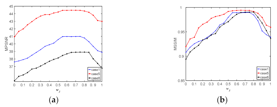
The weighted parameters, w₁, w_2, and w_3, were used to balance the weights of spatial TV and SSRTV. It was demonstrated in [12] that the two weights of spatial TV can be set the same; so, we set w₁ = w₂ = 1. Then, we tuned the weight of SSRTV in the range of 0 to 1. The parameter w₃ was crucial in keeping the balance of the local spatial smoothness and local spatial-spectral smoothness. Figure 18 plots the curves of MPSNR and MSSIM values with respect to parameter w₃; it can be observed that when the parameter w₃ was in the range of 0.6 to 0.8, the MPSNR and MSSIM achieved the best values. Therefore, we set w₃ = 0.7 in all the experiments.

(2)

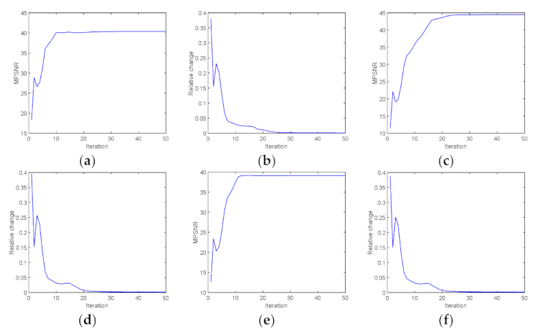
Convergence Analysis

Due to the non-convex constraint of LRTD, our solver was a non-convex optimization problem. Therefore, it was hard to get the globally optimal solution, and theoretical proof of the convergence was hard to guarantee. Nevertheless, to promote convergence of the algorithm, we employed the ALM-based optimization [39] strategy to update the penalty parameter μ in each iteration. Additionally, we illustrated the convergence of our solver by means of empirical analysis. The MPSNR and the relative change of the $\frac{\Vert {\mathcal{X}}^{(k + 1)} - {\mathcal{X}}^{\left(k\right)}\Vert \stackrel{2}{F}}{\Vert {\mathcal{X}}^{\left(k\right)}\Vert \stackrel{2}{F}}$ values gain versus the iteration number under case 1, case 5, and case 6 in the simulated experiment are presented in Figure 18. It can be recognized that, with the increasing of iterations, even if there were significant jumps in all the subfigures in Figure 19, the MPSNR values increased rapidly before gradually stabilizing to a value, and the relative change converged to zero after about 20 iterations. This clearly illustrated the convergent behavior of the proposed LRTDSSRTV solver.

(3)

Operation time analysis

To validate the feasibility and effectiveness of our method, we present the running time of all the compared methods on the real data experiments in

Table 3. Average operation time of different methods under simulated dataset and real dataset (in second).

Dataset	LRMR	LRTV	SSTV	LRTDTV	LRTDGS	LRTDSSRTV
Indian pines	49	93	648	358	263	380
Urban	343	593	2016	768	516	797

. All the experiments were carried out in MATLAB R2016a using a desktop of 16-GB RAM, with Intel Core i5-4590H [email protected] GHz. As shown in Table 3, our method was not the fastest, but the running time was acceptable and our method performed better. In the future, we will design a more effective algorithm to speed up our method.

6. Conclusions

We proposed a new low-rank tensor decomposition-based spatial domain spectral residual total variation-regularized technique for mixed noise removal of HSI. Different from the existing TV regularization methods, both the direct spatial and spatial-spectral piecewise smoothness of an HSI were evaluated by SSRTV, leading to an effective way to remove Gaussian noise for HSI. Additionally, the global spatial-spectral correlation of clean HSI among all bands was described via low-rank tensor decomposition, which can aid in isolating the sparse noise from the clean HSI. Moreover, the l_2,1 norm was more effective for removing the sparse noise, especially the structure sparse noise. We also formulated SSRTV-regularized HSI restoration as a constrained non-convex optimization problem and developed an efficient algorithm based on ADMM. Experimental results on mixed noise removal based on simulated data and real data validated the efficiency and utility of SSRTV. In the future, we will attempt to exploit more potential priori for the difference image to further improve the HSI restoration results.

References

1. Bioucas-Dias, J.M.; Plaza, A.; Camps-Valls, G.; Scheunders, P.; Nasrabadi, N.; Chanussot, J. Hyperspectral remote sensing data analysis and future challenges. IEEE Geosci. Remote Sens. Mag. 2013, 1, 6–36. [Google Scholar] [CrossRef] [Green Version]
2. Zhang, H.; He, W.; Zhang, L.; Shen, H.; Yuan, Q. Hyperspectral Image Restoration Using Low-Rank Matrix Recovery. IEEE Trans. Geosci. Remote Sens. 2014, 52, 4729–4743. [Google Scholar] [CrossRef]
3. Sun, L.; Wu, Z.; Xiao, L.; Liu, J.; Wei, Z.; Dang, F. A novel l 1/2 sparse regression method for hyperspectral unmixing. Int. J. Remote Sens. 2013, 34, 6983–7001. [Google Scholar] [CrossRef]
4. Sun, L.; Wang, S.; Wang, J.; Zheng, Y.; Jeon, B. Hyperspectral classification employing spatial–spectral low rank representation in hidden fields. J. Ambient. Intell. Humaniz. Comput. 2017, 1–12. [Google Scholar] [CrossRef]
5. Wu, Z.; Shi, L.; Li, J.; Wang, Q.; Sun, L.; Wei, Z.; Plaza, J.; Plaza, A. GPU Parallel Implementation of Spatially Adaptive Hyperspectral Image Classification. IEEE J. Sel. Top. Appl. Earth Obs. Remote Sens. 2017, 11, 1131–1143. [Google Scholar] [CrossRef]
6. Xu, Y.; Wu, Z.; Li, J.; Plaza, A.; Wei, Z. Anomaly Detection in Hyperspectral Images Based on Low-Rank and Sparse Representation. IEEE Trans. Geosci. Remote Sens. 2016, 54, 1990–2000. [Google Scholar] [CrossRef]
7. Bollenbeck, F.; Backhaus, A.; Seiffert, U. A multivariate wavelet-PCA denoising-filter for hyperspectral images. In Proceedings of the 2011 3rd Workshop on Hyperspectral Image and Signal Processing: Evolution in Remote Sensing (WHISPERS), Lisbon, Portugal, 6–9 June 2011; pp. 1–4. [Google Scholar]
8. Heo, A.; Lee, J.-H.; Choi, E.-J.; Choi, W.-C.; Kim, S.H.; Park, D.-J. Noise reduction of hyperspectral images using a joint bilateral filter with fused images. In Proceedings of the SPIE—The International Society for Optical Engineering, Orlando, FL, USA, 20 May 2011; p. 80481R. [Google Scholar]
9. Liu, X.; Bourennane, S.; Fossati, C. Denoising of Hyperspectral Images Using the PARAFAC Model and Statistical Performance Analysis. IEEE Trans. Geosci. Remote Sens. 2012, 50, 3717–3724. [Google Scholar] [CrossRef]
10. Green, A.; Berman, M.; Switzer, P.; Craig, M. A transformation for ordering multispectral data in terms of image quality with implications for noise removal. IEEE Trans. Geosci. Remote Sens. 1988, 26, 65–74. [Google Scholar] [CrossRef] [Green Version]
11. Elad, M.; Aharon, M. Image denoising via sparse and redundant representations over learned dictionaries. IEEE Trans. Image Processing 2006, 15, 3736–3745. [Google Scholar] [CrossRef] [PubMed]
12. Wang, Y.; Peng, J.; Zhao, Q.; Leung, Y.; Zhao, X.-L.; Meng, D. Hyperspectral Image Restoration Via Total Variation Regularized Low-Rank Tensor Decomposition. IEEE J. Sel. Top. Appl. Earth Obs. Remote Sens. 2018, 11, 1227–1243. [Google Scholar] [CrossRef] [Green Version]
13. Karami, A.; Yazdi, M.; Asli, A.Z. Noise Reduction of Hyperspectral Images Using Kernel Non-Negative Tucker Decomposition. IEEE J. Sel. Top. Signal Processing 2011, 5, 487–493. [Google Scholar] [CrossRef]
14. Peng, Y.; Meng, D.; Xu, Z.; Gao, C.; Yang, Y.; Zhang, B. Decomposable Nonlocal Tensor Dictionary Learning for Multispectral Image Denoising. In Proceedings of the 2014 IEEE Conference on Computer Vision and Pattern Recognition, Columbus, OH, USA, 24–27 June 2014; pp. 2949–2956. [Google Scholar]
15. Othman, H.; Qian, S.-E. Noise reduction of hyperspectral imagery using hybrid spatial-spectral derivative-domain wavelet shrinkage. IEEE Trans. Geosci. Remote Sens. 2006, 44, 397–408. [Google Scholar] [CrossRef]
16. Zhao, Y.-Q.; Yang, J. Hyperspectral Image Denoising via Sparse Representation and Low-Rank Constraint. IEEE Trans. Geosci. Remote Sens. 2015, 53, 296–308. [Google Scholar] [CrossRef]
17. Yuan, Q.; Zhang, L.; Shen, H. Hyperspectral Image Denoising Employing a Spectral–Spatial Adaptive Total Variation Model. IEEE Trans. Geosci. Remote Sens. 2012, 50, 3660–3677. [Google Scholar] [CrossRef]
18. Chen, Y.; Guo, Y.; Wang, Y.; Wang, D.; Peng, C.; He, G. Denoising of Hyperspectral Images Using Nonconvex Low Rank Matrix Approximation. IEEE Trans. Geosci. Remote Sens. 2017, 55, 5366–5380. [Google Scholar] [CrossRef]
19. Xie, Y.; Qu, Y.; Tao, D.; Wu, W.; Yuan, Q.; Zhang, W. Hyperspectral image restoration via iteratively regularized weighted Schatten p-norm minimization. IEEE Trans. Geosci. Remote Sens. 2016, 54, 4642–4659. [Google Scholar] [CrossRef]
20. Xie, Y.; Gu, S.; Liu, Y.; Zuo, W.; Zhang, W.; Zhang, L. Weighted Schatten p-norm minimization for image denoising and background subtraction. IEEE Trans. Image Processing 2016, 25, 4842–4857. [Google Scholar] [CrossRef] [Green Version]
21. He, W.; Zhang, H.; Zhang, L.; Shen, H. Total-Variation-Regularized Low-Rank Matrix Factorization for Hyperspectral Image Restoration. IEEE Trans. Geosci. Remote Sens. 2016, 54, 178–188. [Google Scholar] [CrossRef]
22. Zheng, X.; Yuan, Y.; Lu, X. Hyperspectral Image Denoising by Fusing the Selected Related Bands. IEEE Trans. Geosci. Remote Sens. 2018, 57, 2596–2609. [Google Scholar] [CrossRef]
23. Aggarwal, H.K.; Majumdar, A. Hyperspectral Image Denoising Using Spatio-Spectral Total Variation. IEEE Geosci. Remote Sens. Lett. 2016, 13, 442–446. [Google Scholar] [CrossRef]
24. He, W.; Zhang, H.; Shen, H.; Zhang, L. Hyperspectral Image Denoising Using Local Low-Rank Matrix Recovery and Global Spatial–Spectral Total Variation. IEEE J. Sel. Top. Appl. Earth Obs. Remote Sens. 2018, 11, 713–729. [Google Scholar] [CrossRef]
25. Sun, L.; Jeon, B.; Zheng, Y.; Wu, Z. A Novel Weighted Cross Total Variation Method for Hyperspectral Image Mixed Denoising. IEEE Access 2017, 5, 27172–27188. [Google Scholar] [CrossRef]
26. Fan, H.; Li, C.; Guo, Y.; Kuang, G.; Ma, J. Spatial–Spectral Total Variation Regularized Low-Rank Tensor Decomposition for Hyperspectral Image Denoising. IEEE Trans. Geosci. Remote Sens. 2018, 56, 6196–6213. [Google Scholar] [CrossRef]
27. Huang, Z.; Li, S.; Fang, L.; Li, H.; Benediktsson, J.A. Hyperspectral Image Denoising With Group Sparse and Low-Rank Tensor Decomposition. IEEE Access 2017, 6, 1380–1390. [Google Scholar] [CrossRef]
28. Takeyama, S.; Ono, S.; Kumazawa, I. Mixed Noise Removal for Hyperspectral Images Using Hybrid Spatio-Spectral Total Variation. In Proceedings of the 2019 IEEE International Conference on Image Processing (ICIP), Taipei, Taiwan, 22–25 September 2019; pp. 3128–3132. [Google Scholar]
29. Yuan, Y.; Zheng, X.; Lu, X. Spectral–Spatial Kernel Regularized for Hyperspectral Image Denoising. IEEE Trans. Geosci. Remote Sens. 2015, 53, 3815–3832. [Google Scholar] [CrossRef]
30. Kolda, T.; Bader, B.W. Tensor Decompositions and Applications. SIAM Rev. 2009, 51, 455–500. [Google Scholar] [CrossRef]
31. Huang, Y.-M.; Yan, H.-Y.; Zeng, T. Multiplicative Noise Removal Based on Unbiased Box-Cox Transformation. Commun. Comput. Phys. 2017, 22, 803–828. [Google Scholar] [CrossRef]
32. Chen, Y.; He, W.; Yokoya, N.; Huang, T.-Z. Hyperspectral Image Restoration Using Weighted Group Sparsity-Regularized Low-Rank Tensor Decomposition. IEEE Trans. Cybern. 2019, 50, 3556–3570. [Google Scholar] [CrossRef] [PubMed]
33. Zhu, R.; Dong, M.; Xue, J.-H. Spectral Nonlocal Restoration of Hyperspectral Images With Low-Rank Property. IEEE J. Sel. Top. Appl. Earth Obs. Remote Sens. 2015, 8, 3062–3067. [Google Scholar] [CrossRef]
34. He, W.; Zhang, H.; Zhang, L.; Shen, H. Hyperspectral Image Denoising via Noise-Adjusted Iterative Low-Rank Matrix Approximation. IEEE J. Sel. Top. Appl. Earth Obs. Remote Sens. 2015, 8, 3050–3061. [Google Scholar] [CrossRef]
35. Xu, H.; Caramanis, C.; Sanghavi, S. Robust PCA via Outlier Pursuit. IEEE Trans. Inf. Theory 2012, 58, 3047–3064. [Google Scholar] [CrossRef] [Green Version]
36. Liu, G.; Lin, Z.; Yan, S.; Sun, J.; Yu, Y.; Ma, Y. Robust Recovery of Subspace Structures by Low-Rank Representation. IEEE Trans. Pattern Anal. Mach. Intell. 2013, 35, 171–184. [Google Scholar] [CrossRef] [PubMed] [Green Version]
37. Bioucas-Dias, J.M.; Plaza, A.; Dobigeon, N.; Parente, M.; Du, Q.; Gader, P.; Chanussot, J. Hyperspectral Unmixing Overview: Geometrical, Statistical, and Sparse Regression-Based Approaches. IEEE J. Sel. Top. Appl. Earth Obs. Remote Sens. 2012, 5, 354–379. [Google Scholar] [CrossRef] [Green Version]
38. Boyd, S.; Parikh, N.; Chu, E. Distributed Optimization and Statistical Learning via the Alternating Direction Method of Multipliers. Found. Trends Mach. Learn. 2010, 3, 1–122. [Google Scholar] [CrossRef]
39. Feng, P.; Ling, B.W.; Lei, R.; Chen, J. Singular spectral analysis-based denoising without computing singular values via augmented Lagrange multiplier algorithm. IET Signal Processing 2019, 13, 149–156. [Google Scholar] [CrossRef]
40. Wang, Q.; Wu, Z.; Jin, J.; Wang, T.; Shen, Y. Low rank constraint and spatial spectral total variation for hyperspectral image mixed denoising. Signal Processing 2018, 142, 11–26. [Google Scholar] [CrossRef]
41. Wang, Z.; Bovik, H.C.; Sheikh, H.R.; Simoncelli, E.P. Image Quality Assessment: From Error Visibility to Structural Similarity. IEEE Trans. Image Processing 2004, 13, 600–612. [Google Scholar] [CrossRef] [Green Version]
42. Kong, X.; Zhao, Y.; Xue, J.; Chan, J.C.-W.; Kong, S.G. Global and Local Tensor Sparse Approximation Models for Hyperspectral Image Destriping. Remote Sens. 2020, 12, 704. [Google Scholar] [CrossRef] [Green Version]
43. Toksoz, M.A.; Ulusoy, I. Hyperspectral Image Classification via Basic Thresholding Classifier. IEEE Trans. Geosci. Remote Sens. 2016, 54, 4039–4051. [Google Scholar] [CrossRef]
44. Bioucas-Dias, J.; Nascimento, J. Hyperspectral Subspace Identification. IEEE Trans. Geosci. Remote Sens. 2008, 46, 2435–2445. [Google Scholar] [CrossRef] [Green Version]
Figure 1. Examples of differences between 3DTV and SSTV with Band 115 of real Urban dataset. The 3DTV calculates the L1 norm of spatial-spectral differences (blue line). SSRTV evaluates the L1 norm of both direct spatial and spatial-spectral residual differences (red line). The D h X , D v X and D p X in (ac) respectively represent differences of X along the horizontal, vertical, and spectral directions. The D h D p X and D v D p X in (d) and (e) represent differences of D p X along the horizontal and vertical directions.
Remotesensing 14 00511 g001
Figure 2. The histogram of (a) D p X , (b) D h D p X ,   and (c) D v D p X .
Remotesensing 14 00511 g002
Figure 3. Illustration of deadlines and stripes in Urban data. (a) Band 204. (b) Band 206.
Remotesensing 14 00511 g003
Figure 4. The flowchart of the LRTDSSRTV model.
Remotesensing 14 00511 g004
Figure 5. Denoised results of all the methods: (a) Original band 46. (b) Noisy band under case 1. (c) LRMR. (d) LRTV. (e) SSTV. (f) LRTDTV. (g) LRTDGS. (h) LRTDSSRTV.
Remotesensing 14 00511 g005
Figure 6. Denoised results of all the methods: (a) Original band 168. (b) Noisy band in case 5. (c) LRMR. (d) LRTV. (e) SSTV. (f) LRTDTV. (g) LRTDGS. (h) LRTDSSRTV.
Remotesensing 14 00511 g006
Figure 7. Denoised results of all the methods: (a) Original band 162. (b) Noisy band in case 6. (c) LRMR. (d) LRTV. (e) SSTV. (f) LRTDTV. (g) LRTDGS. (h) LRTDSSRTV.
Remotesensing 14 00511 g007
Figure 8. Detailed PSNR/SSIM evaluation of all the methods for each band: (a,b) Case 1, (c,d) Case 2, (e,f) Case 3, (g,h) Case 4, (i,j) Case 5, (k,l) Case 6.
Remotesensing 14 00511 g008aRemotesensing 14 00511 g008b
Figure 9. From top to bottom are the differences between the original spectrum and the restoration results of locations (86, 75), (55, 90), and (115, 102) in the spatial domain on the Indian Pines’ dataset in cases 1, 5, and 6, respectively. (a) Noisy. (b) LRMR. (c) LRTV. (d) SSTV (e) LRTDTV. (f) LRTDGS. (g) LRTDSSRTV.
Remotesensing 14 00511 g009aRemotesensing 14 00511 g009b
Figure 10. Restoration results of all comparison methods for band 104 of the real Indian Pines’ dataset. (a) Original. (b) LRMR. (c) LRTV. (d) SSTV. (e) LRTDTV. (f) LRTDGS. (g) LRTDSSRTV.
Remotesensing 14 00511 g010
Figure 11. Restoration results of all comparison methods for band 150 of the real Indian Pines’ dataset. (a) Original. (b) LRMR. (c) LRTV. (d) SSTV. (e) LRTDTV. (f) LRTDGS. (g) LRTDSSRTV.
Remotesensing 14 00511 g011
Figure 12. Restoration results of all comparison methods for band 108 of the real Urban dataset. (a) Original. (b) LRMR. (c) LRTV. (d) SSTV. (e) LRTDTV. (f) LRTDGS. (g) LRTDSSRTV.
Remotesensing 14 00511 g012
Figure 13. Spectral signatures’ curve of band 108 for the real Urban dataset estimated by different methods: (a) Original. (b) LRMR. (c) LRTV. (d) SSTV. (e) LRTDTV. (f) LRTDGS. (g) Proposed.
Remotesensing 14 00511 g013
Figure 14. Restoration results of all comparison methods for band 208 of the real Urban dataset. (a) Original. (b) LRMR. (c) LRTV. (d) SSTV. (e) LRTDTV. (f) LRTDGS. (g) LRTDSSRTV.
Remotesensing 14 00511 g014
Figure 15. Spectral signatures’ curve of band 208 for the real Urban dataset estimated by different methods: (a) Original. (b) LRMR. (c) LRTV. (d) SSTV. (e) LRTDTV. (f) LRTDGS. (g) LRTDSSRTV.
Remotesensing 14 00511 g015
Figure 16. Classification map on Indian pines’ dataset, (a) true values, (b) before denoising, (c) LRMR, (d) LRTV, (e) SSTV, (f) LRTDTV, (g) LRTDGS, (h) SSRTV.
Remotesensing 14 00511 g016
Figure 17. Sensitivity analysis between parameters ρ and τ using the simulated Indian Pines’ dataset. (a) Case 1. (b) Case 5. (c) Cases 6.
Remotesensing 14 00511 g017
Figure 18. Performance with weight parameter w3. (a) MPSNR value vs. w3, (b) MSSIM value vs. w3.
Remotesensing 14 00511 g018
Figure 19. MPSNR and relative change values versus the iteration number of LRTDSSRTV: (a,b) for case 1; (c,d) for case 5; (e,f) for case 6.
Remotesensing 14 00511 g019