Article

Analysis of Permafrost Distribution and Change in the Mid-East Qinghai–Tibetan Plateau during 2012–2021 Using the New TLZ Model

Graduate School of Science and Engineering, Ibaraki University, Hitachi 316-8511, Ibaraki, Japan
*
Author to whom correspondence should be addressed.
Remote Sens. 2022, 14(24), 6350; https://doi.org/10.3390/rs14246350
Submission received: 20 November 2022 / Revised: 9 December 2022 / Accepted: 13 December 2022 / Published: 15 December 2022
(This article belongs to the Special Issue Remote Sensing and Land Surface Process Models for Permafrost Studies)

Abstract

:
The monitoring of permafrost is important for assessing the effects of global environmental changes and maintaining and managing social infrastructure, and remote sensing is increasingly being used for this wide-area monitoring. However, the accuracy of the conventional method in terms of temperature factor and soil factor needs to be improved. To address these two issues, in this study, we propose a new model to evaluate permafrost with a higher accuracy than the conventional methods. In this model, the land surface temperature (LST) is used as the upper temperature of the active layer of permafrost, and the temperature at the top of permafrost (TTOP) is used as the lower temperature. The TTOP value is then calculated by a modified equation using precipitation–evapotranspiration (PE) factors to account for the effect of soil moisture. This model, referred to as the TTOP-LST zero-curtain (TLZ) model, allows us to analyze subsurface temperatures for each layer of the active layer, and to evaluate the presence or absence of the zero-curtain effect through a time series analysis of stratified subsurface temperatures. The model was applied to the Qinghai–Tibetan Plateau and permafrost was classified into seven classes based on aspects such as stability and seasonality. As a result, it was possible to map the recent deterioration of permafrost in this region, which is thought to be caused by global warming. A comparison with the mean annual ground temperature (MAGT) model using local subsurface temperature data showed that the average root mean square error (RMSE) value of subsurface temperatures at different depths was 0.19 degrees C, indicating the validity of the TLZ model. A similar analysis based on the TLZ model is expected to enable detailed permafrost analysis in other areas.

1. Introduction

Permafrost is generally defined as rocks and soils rich in ice with a temperature of below zero degrees [1,2]. As an important component of the cryosphere, one of the five global spheres, permafrost covers a large global land surface area [3], and approximately 50 × 106 km2 of the global land surface soil undergoes a freeze–thaw transition every year [4]. Permafrost, seasonal permafrost, and ephemeral permafrost are classified according to the time period during which the permafrost remains frozen. Permafrost is defined when the freezing period lasts for more than two years [5]. The active layer is defined as the layer of rock and soil above the permafrost layer that melts in the warm season and freezes in the cold season. The deepening of the active layer is considered to be a sign of permafrost degradation [6,7]. The active layer is also the main site of hydrothermal, gaseous and energy exchange between permafrost and the outside world [8,9]. The energy exchange in the active layer of permafrost is influenced by many factors such as vegetation cover, snow cover, air temperature, geotechnical properties, soil moisture, unfrozen water content, precipitation, evapotranspiration, and geomorphology [10,11,12].
In recent years, global warming caused by the greenhouse effect has directly led to the deepening of the active layer of permafrost over large areas, and warnings of permafrost degradation have been issued [13,14,15,16]. The remarkable hydrothermal energy changes in the active layer have led to the degradation of the permafrost [17,18], as well as to a series of environmental problems, such as a significant reduction in the area of vegetation [19], a decrease in the microbial diversity and stability of the soil, an increase in the emission of organic matter containing carbon elements in the soil [20,21,22,23], an increase in precipitation [24,25], and warmer winters [26]. Therefore, based on an accurate grasp of the variation patterns in temperature and soil factors, it is important to carry out high-resolution spatial mapping, long-period dynamic monitoring, and a high-frequency analysis of permafrost-related changes in the thickness of the active permafrost layer.
In the early 1990s, permafrost research was mainly carried out by teams in the field [27], using field surveys and boreholes to obtain local data based on the distribution and nature of permafrost, but this approach is limited by geographical and economic factors, which hinder long-period permafrost research across a wide area. Such small-scale and limited field data restrict the study of permafrost to a crude planimetric stage during this period. To address the limitations of fieldwork, scientists have proposed a variety of physical, empirical, semi-empirical, and semi-physical models for permafrost research based on the principles of physics and prior research experience. With the continued development and improvement of remote sensing technology in the 21st century, the research method of combining semi-empirical and semi-physical models with remote sensing data has become the most popular approach to permafrost research. In particular, the following permafrost models and the recent examples of permafrost research are most representative of this approach: the Stefan model [28,29], the Nelson model [30,31,32,33,34], the Kudryavtsev model [35,36], the mean annual ground temperature (MAGT) model [37,38], the temperature at the top of the permafrost (TTOP)-MAAT model [39,40,41,42,43,44,45,46,47], the LST–zero-curtain model [48,49,50,51], etc. These models are applicable to the study of permafrost at different temporal and spatial scales, and each has its own advantages and limitations.
The Stefan model [28] was first proposed by Josef Stefan in 1891 to study the freezing and thawing process of Arctic lake ice to calculate its thickness, and in 1943, Berggren [29] studied soil ice instead of pure lake ice, using the parameters and properties of the soil to calculate the thickness of the active layer in the permafrost region to derive the general permafrost distribution. In 1983, Nelson et al. introduced a freeze–thaw index factor based on Stefan’s permafrost model and proposed the Nelson model [30] or the Nelson freeze–thaw index model. However, this model struggles to determine the unfrozen water content of soils on a large spatial scale. In the following decades, Nelson et al. carried out a series of factor improvements to the Nelson model [31,32,33,34], which made the Nelson model more applicable at high latitudes without taking into account the influence of vegetation and snow. Overall, the Stefan and Nelson models are large-scale permafrost distribution prediction models that are mainly influenced by soil properties, elevation and latitude and longitude. In practice, however, the distribution of permafrost is also influenced to a large extent by climatic and geographic factors at small and medium scales, and the applicability of these two models is not particularly high for studies of permafrost distribution that require a high accuracy.
In 1974, Kudryavtsev proposed the Kudryavtsev model [35] based on the influence of climate and temperature on permafrost to address the shortcomings of the Stefan model in permafrost research. The Kudryavtsev model analyzes the permafrost system in layers according to the thermal condition of the soil, taking into full consideration the influence of temperature and soil water content on the permafrost. This model advantageously takes into account the heat transfer processes between the soil and the atmosphere in the permafrost region in a more comprehensive way. This model has been used in the Kuparuk region of northern Alaska, USA [36], but it is less commonly used than other models for permafrost research, mainly because the number of parameters required in the model can easily lead to errors in the simulation between layers.
The MAGT model [37] was proposed by Nan et al. in 2005 in a study on the prediction of future permafrost distribution in the Tibetan Plateau region, where MAGT can be generally understood as the ground temperature at the depth where the annual difference in permafrost ground temperature is zero. This model is based on decades of borehole measurements along the eastern part of the Qinghai–Tibetan Plateau, and was developed by linearly regressing the temperature data at different depths with the latitude and elevation information of the study area, as the threshold value to distinguish between permafrost and non-permafrost. The MAGT model was successfully applied in subsequent studies on permafrost distribution on the Tibetan Plateau by Qin et al. [15] in 2017 and Aalto et al. [38] in 2018. The advantages of this model are that it is based on long-period ground temperature data at different depths and takes into account the geographic information of the Tibetan Plateau region. The model results are more reliable and can be used to compare the results of other models for a permafrost analysis in the Tibetan Plateau region. The model is, however, not applicable to areas where there are no actual measurement data.
The TTOP model, proposed by Smith and Riseborough in 1996, is a semi-empirical and semi-physical analysis model for permafrost that analyzes the energy balance and conversion relationship between permafrost and climate [39]. Using the temperature difference between the ground temperature and air temperature and the different thermal conductivity of the soil during freezing and thawing periods, the model analyzes the relationship between temperature and air temperature at the top of the permafrost layer in multi-year permafrost from the perspective of negative temperature displacement after removing the effects of vegetation cover and snow cover. In 2002, Riseborough corrected the TTOP model for the freezing period [40], and in the following two decades, the TTOP model was successfully applied in Canada [41], Norway [42], the Daxinganling in northeastern China [43], the Qinghai–Tibetan Plateau in China [44,45,46], and the Northern Hemisphere as a whole [47]. The TTOP model, compared to the Stefan and Nelson models, fully takes into account soil properties and the freeze–thaw state of the permafrost. Compared to the Stefan and Nelson models, the TTOP model takes into account the influence of temperature, vegetation and snow cover, and can be applied to small- and medium-scale permafrost studies. Compared to the MAGT model, the TTOP model has a higher applicability in the absence of measured data. However, in previous studies [41,42,43,44,45,46,47], satellite data and measurements of the land surface temperature (LST), air temperature, vegetation impact, snow impact, soil properties and other parameters used in the TTOP model were mostly large-scale observations with a low resolution, rather than daily monitoring data or high-resolution observations, and there is room for improvement in the processing of the data. Moreover, the soil thermal conductivity used assumes that the soil water content is saturated, but in fact, due to the annual freeze–thaw state of the active layer and differences in precipitation and evapotranspiration, the soil water content is not constant even if the soil composition does not change. Additionally, the TTOP model mostly combines the annual average air temperature in the range of 2–10 m to determine the presence of permafrost, and the wide spatial range of temperature is prone to observation errors. These are the areas where the TTOP model needs to be improved.
In 2020, Gillespie et al. proposed to identify and map the geothermal isothermal period during freeze–thaw of active permafrost, i.e., the zero-curtain period, using MODIS LST images, and use it as a key interval for permafrost determination [48]. In this study, this approach is referred to as the LST–zero-curtain model. In the science of permafrost, the physical phenomenon that keeps the active layer of permafrost at or near 0 °C for a certain period of time due to the latent heat of the soil during the freezing or thawing process is called the zero-curtain effect [49]. When the zero-curtain effect occurs in the freezing (autumn) or thawing (spring) period of the active permafrost layer, the energy that would change the soil temperature does not directly change the temperature of the active soil, but rather freezes the groundwater or melts the ground ice in the active layer [50]. Therefore, the length of time that the zero-curtain phenomenon is maintained in the freezing or thawing period of each year, where the freezing period is generally much longer than the thawing period in the same year, can be used to characterize the presence or stability of permafrost. The use of the zero-curtain effect to characterize permafrost largely excludes the influence of geographic properties, such as soil, ice, and water heat conductivity. For example, Gillespie et al. demonstrated that the zero-curtain period was consistently identified in MODIS LST data based on the principle of the zero-curtain effect by spatially transforming the temperature of long-period LST with a 2–40 cm subsurface in the permafrost zone of the Atacama Andes, Chile [48]. The LST–zero-curtain model pioneered a new approach to identify and map permafrost using long-period MODIS LST images. However, the average thickness of most active permafrost layers is about 3 m [52]. In Gillespie et al.’s study, the zero-curtain effect was estimated by the LST–zero-curtain model at only about 40 cm below ground level without completely removing the influence of vegetation and snow [48], which should be improved in accuracy, because the zero-curtain effect may occur deeper below the ground, also often covered by vegetation or snow. In addition, the determination of the zero-curtain from the LST alone may introduce errors because it does not take into account the lower-limit temperature. This means that the LST–zero-curtain model has some limitations, and there is room for improvement.
As mentioned above, both the TTOP model and the LST–zero-curtain model have been successfully used to analyze permafrost distribution by characterizing soil energy changes through temperature differences, but they have several problems that must be resolved. Therefore, this study proposes a TTOP LST–zero-curtain (TLZ) model that changes the upper-limit temperature from the ground air-temperature used in the conventional TTOP models to LST and uses a modified TTOP as the lower-limit temperature. This model is expected to be able to determine the zero-curtain effect with a higher accuracy than the conventional LST–zero-curtain model. To validate the model, we applied it to the mid-east part of the Qinghai–Tibetan Plateau and discuss the results.

2. Materials and Methods

2.1. Study Area and Data Sources

The Qinghai–Tibetan Plateau is the source of the Yangtze and Yellow Rivers, and large amounts of snow and glaciers nurture these rivers. This plateau has an area of 1.05 × 10⁶ to 1.5 × 10⁶ km2 [53] and is the largest plateau-type permafrost distribution area in Asia, as well as the largest and highest permafrost distribution area in the world [54]. This plateau has unique geographical and climatic attributes. From north to south, it can be divided into a plateau cold climate zone, plateau cold zone, plateau temperate zone, and subtropics and tropics. The vegetation distribution from northwest to southeast comprises grassland, meadow, shrubland and forest, and most areas have a large daily difference in temperature and precipitation gradually increases from north to south. Therefore, the plateau is also known as an initiation zone of climate change [55], and the stability and sustainability of permafrost in this region have immeasurable practical significance for climate and environmental balance in Asia and through the world.
The Qinghai–Tibetan Plateau is a combination of plateau surface, swamp, water system and many mountain ranges, including the world’s highest peak of Mount Everest. There are dozens of large and small mountain ranges, which run in a north–south and east–west direction. The overall terrain shows a trend of low southeast and high northwest, and the average altitude of the northwest region exceeds 5000 m [56], which is not convenient for long-period continuous geographic observation research. Compared with the northwest part of the plateau, the mid-east part of the plateau is relatively dense in human activities, with less forest distribution, more precipitation, relatively gentle topographic changes and a concentration of China Meteorological Data Service Centre (CMDC) stations. These stations provide a large amount of measured meteorological data that can be used for validation, compared to the other areas of the plateau. We therefore selected the H25V05 tile of MODIS products included in the mid-east area as the study area.
In Figure 1, the blue polygon indicates the study area, and the red asterisks indicate the locations of the CMDC stations. The area spans from 73°19′ to 104°47′E longitude and 26°00′ to 39°47′N latitude (about 300–1500 km north–south and about 2800 km east–west) [57] and has 54 CMDC stations. We also divided the study area into six subareas, A, B, C, D, E and F, as shown in the figure.
The main data that we used were a variety of MODIS products and various data observed by CMDC stations. All of the MODIS products used were downloaded from the National Aeronautics and Space Administration (NASA) website (https://ladsweb.modaps.eosdis.nasa.gov/ (accessed on 7 July 2022)). The used CMDC data were meteorological and subsurface data that were obtained from the site of the China Meteorological Administration (http://data.cma.cn/en (accessed on 7 July 2022)).

2.2. Methodology

2.2.1. Modification of the TTOP Model

In the J model proposed by Johansen in 1975, soil thermal conductivity was obtained by integrating the effects of saturation correlation coefficient, soil thermal conductivity at saturation, and dry soil thermal conductivity [58], and many investigators used the value of the J model in permafrost analysis using TTOP for the Tibetan Plateau. In the J model, a saturated soil water content was assumed, and the effects of other organic matter and the ice and water mixtures in the soil were considered in classified types of soil. There are more than 30 improved models for the J model in recent years, which are mainly based on the dry soil thermal conductivity, although the soil water content has a great influence on the soil thermal conductivity.
There are three main destinations of precipitation in permafrost areas in general: the first is absorbed by vegetation and snow cover, the second is absorbed by the residual soil in the active layer, and the third is converted to groundwater seepage. The component that really affects soil thermal conductivity is the net soil water content remaining in the active layer soil [59]. Therefore, in the present study, we propose a modified TTOP model that includes the relevant net water content effect of the active layer for each of the thawing and freezing periods using the soil water content, precipitation, and evapotranspiration measured by the China Meteorological Administration. We also consider the influence of absorption by the vegetation and snow layers and the influence of groundwater seepage. In this model, the precipitation-evapotranspiration (PE) factors pet and pef for each of the freezing and thawing periods are added on the basis of the J model to dynamically reflect the water content factors; therefore, this model is expected to more accurately express the year-to-year variation of the soil thermal conductivity. The modified TTOP is expressed as:
T T O P = A t   ·   C t   ·   s t   ·   p e t A f   ·   C f   ·   s f   ·   p e f s f   ·   p e f   ·   Y
where subscripts t and f indicate thawing and freezing periods, respectively, Y is the number of days per year (365 or 366), A is cumulative temperature factor, C is reciprocal of vegetation or snow cover fraction, s is soil thermal conductivity [W/m/°C], and pe is the PE factor. The soil thermal conductivity corrected by the PE factors can be given by St = ts × pet and Sf = tf × pef (referred to as corrected soil thermal conductivity).
The value of At is given by the sum of all daily mean temperatures above 0 °C, and that of Af is given by the sum of all absolute daily mean temperatures below 0 °C, when daily temperature data for the entire year of interest are available for the location of interest.
The PE factors are given by:
p e t = w t p t ( e t + c t + g t ) = w t s w t
p e f = w f p f ( e f + c f + g f ) = w f s w f
where w is net soil water content, respectively, p is precipitation, e is potential soil evapotranspiration, c is vegetation or snow cover influence factor, g is groundwater seepage factor, and sw is saturated soil water content.
The values of st and sf in the study area can be referred to as the reported values in the J model as shown by Table 1 [58]. We employed the maximum (=2.92) and minimum (=1.15) values, except for organic matter, in the table for st and sf in the analysis of this study.

2.2.2. Permafrost Analysis Based on the TLZ Model

The TLZ model described in the following step 4 enables the location of pixels to be mapped where the zero-curtain effect is present and the approximate depth at which this effect occurs. Based on this model, the permafrost analysis in this study was conducted as follows:
  • The annual TTOP for each pixel in the study area was calculated (all TTOP values described in this section were determined by the modified formula presented in Section 2.2.1). Pixels with an annual TTOP > 0 were assumed to be non-permafrost, and only permafrost pixels that had an annual TTOP < 0 were processed thereafter.
  • Based on the annual temperature data for the study area, the thawing season was set from May to September and the freezing season from October to April. Then, seasonal TTOP (TTOPt, TTOPf) for each season was calculated for each permafrost pixel. Pixels that satisfied “TTOPt < 0 < TTOPf” were assumed to melt in summer and freeze in winter during the course of a year, e.g., it can be assumed that the zero-curtain phenomenon occurs. Therefore, only pixels that satisfy this condition were extracted, and others were excluded. Note that among the excluded pixels, those that satisfy TTOPf < 0 can be regarded as stable permafrost because they have not thawed during the summer.
  • During the thawing period, the ice melts, so the LST has an overall positive value. Conversely, during the freezing season, the ice freezes, and LST has a negative value as a whole. Therefore, although it is affected by errors, coverage, and daily variations in LST, the overall relationship can be assumed to be “TTOPt < 0 and LST > 0” for the thawing period and “TTOPf > 0 and LST < 0” for the freezing period. Therefore, only pixels satisfying these conditions were extracted, and others were excluded.
  • For the pixels extracted in (3), we assume that the subsurface temperature between the ground surface and the lower surface of the active layer linearly varied between LST and the seasonal TTOP, and calculated the depth at which the subsurface temperature was within 0 ± 0.1 °C (since the signs of the seasonal TTOP and LST are opposite, a solution must exist), where a uniform depth (3 m) was assumed for the depth below the active layer in the study area, based on the study by Wang et al. [52]. The determined depth can be treated as the zero-curtain depth. In this study, this approach is referred to as the TLZ model. Figure 2 shows a conceptual diagram of the TLZ model.
Details of the above procedure are described in the next section.

2.3. Data Used and Parameter Determination

2.3.1. Cumulative Temperature Factor (At and Af)

In order to determine the cumulative temperature factors At and Af in the thawing and freezing periods in the TTOP model, Kukkonen et al. (2020) used a method involving extreme monthly temperatures [60]. Although this method takes into account a certain degree of temperature amplitude, there is still a large error due to the analysis of the annual freeze–thaw temperature using only two months of data. Essentially, there is a difference between the annual variation in extreme temperatures and the annual mean temperature, which is more evident in the multi-year study cycle. In addition, temperature data given to 54 meteorological stations were obtained from the daily temperature data observed by the China’s Fengyun meteorological satellite, and are inevitable small periods of missing data and data anomalies.
In the present paper, for a higher accuracy, we prepared the air temperature data as follows. First, the 54 CMDC stations were divided into six groups corresponding to subareas A, B, C, D, E, and F in Figure 1, and for each group, air temperature data within 2–10 m of the ground surface for 2012–2021 were collected. Missing temperature data were supplemented using averages of 3 days for each group after the removal of outliers. Next, these data were used for calculation of the mean annual air temperature value in the study area for each year from 2012 to 2021. In this calculation, spatial interpolation was performed by establishing buffers for the temperature at 54 stations, using the thin plate spline method [61]. Finally, we performed a positive and negative cumulative temperature calculations on the air temperature data with the error values removed and determined the At and Af factors.

2.3.2. Reciprocal of Vegetation Cover Fraction (Ct)

In order to analyze the permafrost region in the Daxinganling Mountains, China, Zhang et al. [43] used the TTOP model. However, since vegetation effects during freezing and thawing were determined using the MODIS 500/1000 m annual land cover product (MCD12Q1) with only 17 land cover types of the International Geosphere–Biosphere Programme (IGBP), the monthly or daily changes in vegetation cover were not fully considered. Moreover, the IGBP-based land cover types should be reclassified in order to adjust to each study area. Thus, in the present study, we calculated the fraction of vegetation cover (FVC) used for determination of Ct from the normalized difference vegetation index (NDVI) and the enhanced vegetation index (EVI) for each month in the MODIS 250 m/16 day vegetation indices products (MOD13Q1 and MYD13Q1) using the following equation [62]:
FVC = ( V I V I s ) ( V I v V I s )
where VI is vegetation index (NDVI or EVI), and subscripts s and v indicate pure soil and pure vegetation pixels, respectively. Since the confidence interval was set to 0.5% to 99.5%, pixels with soil type accumulation less than 0.5% were dealt as pure soil, and those with grass type accumulation greater than 99.5% were dealt as pure vegetation. The FVC values obtained for NDVI and EVI were combined by the element dichotomous model [62], and the obtained FVC value was used.

2.3.3. Reciprocal of Snow Cover Fraction (Cf)

In the aforementioned study by Zhang et al. [43], since the snow depth was assumed to be a value less than 30 cm and the annual snow factor was set uniformly by a constant value [43], temporal and spatial changes in snow cover were not considered. On the other hand, Jiang et al. (2022) used MODIS surface reflectance daily L2G global 500 m and 1 km products (MOD09GA and MYD09GA) to analyze snow cover in the water tower region, resulting in the root mean square error (RMSE) of 0.14 [63]. Following their study, we used the same products to calculate the fraction of snow cover (FSC) used to determine Cf. In this calculation, we adopted the multiple endmember spectral mixture analysis–automatic–selected endmembers (MESMA-ASE) method proposed by Jiang et al. [63], which provides a reasonable unmixing result by adjusting the type and number of snow endmember spectra of each pixel iteratively based on all endmember combinations in the spectral library.

2.3.4. PE Factors (pet and pef)

The PE factors can be calculated from values of net soil water content, precipitation, potential soil evapotranspiration, vegetation or snow cover influence factor, and groundwater seepage factor in thawing and freezing periods. The net soil water content was given from half-hourly in situ measurements at different depths (5 cm, 50 cm, 150, and 200 cm) by CMDC in the period from 2012 to 2021, the precipitation was given from daily in situ measurements by CMDC in that period, and the evapotranspiration was given from monthly data that CMDC reanalyzed and reprocessed the MODIS/Terra net evapotranspiration 8-day L4 global 500 m SIN grid product (MOD16A2). The vegetation and snow cover influence factors were calculated from FVC and FSC values, respectively. The groundwater seepage factor was given as a constant value by averaging the multiple sets of measurements by Tarnawski et al. (2015) for soil thermal conductivity [64], because in situ measurements were not conducted in the study area.

2.3.5. LST

The LST data used in zero-curtain analysis were given by the MODIS LST/E daily L3 global 1 km SIN grid products (MOD11A1 and MYD11A1) in the period from 2012 to 2021. Data that were missing due to some MODIS observation issues (e.g., Day 50 to 58 in 2016) were supplemented by MODIS LST/E 8-day 1 km products (MOD11A2 and MYD11A2). After supplementing, we combined the MOD11A1 and MYD11A1 datasets, and the daily mean LST maps obtained for the period were used. In order to compare the overall change of LST between 2012 and 2021, the maximum, minimum, mean and standard deviation of LST were calculated and outputted in graphs on a yearly basis.

2.4. Validation Data and Method for Soil Thermal Conductivity

We used the measured soil thermal conductivity data obtained from previous studies based on different research methods to improve the J-model as sample data and performed relevant pre-processing such as resampling and recalculated. The sample data include: McInnes (1981) [65], Hopmans and Dane (1986) [66], Campbell et al. (1994) [67], Côté and Konrad (2005) [68], Kasubuchi et al. (2007) [69], Lu et al. (2007) [70], Chen et al. (2008) [71], Tarnawski et al. (2012) [72], Tarnawski et al. (2015) [64], and McCombie et al. (2017) [73]. The total number of data is 128, of which 64 are in the thawing period and 64 in the freezing period. Those soil types are consistent with any of the types in Table 1, except for organic matter.
The preprocessing was performed considering the differences in soil properties between thawed and frozen soil. The thawed soil samples have a range of properties, including soil particle density, soil porosity, soil dry density, and soil moisture content. In this study, we set the soil particle density to 2500–3000 kg∙m−3, soil porosity coefficient to 0.03–0.07 m, soil dry density to 400–2400 kg∙m−3, and soil water content per unit volume of soil to 0–1, and then determined the range of soil thermal conductivity for the thawed soil samples. The frozen soil samples have soil properties, including temperature, soil bulk density, soil porosity, and unfrozen water content. In this study, we set the temperature in the range from −37 to −1 °C, soil bulk density to 900–2300 kg∙m−3, soil porosity coefficient to 0.02–0.06 m, and unfrozen water content per unit volume of soil to 0–1, and then determined the soil thermal conductivity range for the frozen soil samples. The unfrozen water contents in different frozen soil sample data were adjusted by converting the known water content in each sample and then calculating the ice and unfrozen water content saturation in its corresponding volume based on temperature and empirical equations. For this, the unfrozen water content per unit volume is 0 and 1 for the ice and unfrozen water content saturation, respectively.
Next, we calculated the minimum, maximum, mean, and standard deviation of soil thermal conductivity for thawed and frozen soils determined from the sample data, and used them as validation data for soil thermal conductivity. Similarly, we calculated the statistics of soil thermal conductivity St and Sf with the PE factors in the period 2012–2021 and compared them with those of the validation data.

2.5. Application and Evaluation of TLZ Model

The TLZ model analysis was performed as follows. First, we classified each pixel based on a TTOP value (Equation (1)) as permafrost if TTOP < 0, as transitional permafrost if 0 < TTOP < 0.5, as seasonal permafrost if 0.5 < TTOP < 1.5, and as short-term permafrost/non-permafrost if TTOP > 1.5. Next, the time and location for the occurrence of the zero-curtain effect were determined by a combination of TTOP and LST and analyzed. We then evaluated the stability of each permafrost area by the duration of the zero-curtain effect. Permafrost areas where the zero-curtain effect lasted (a) 1–2 weeks, (b) 2–3 weeks, (c) 3–4 weeks, and (d) 4 or more weeks were classified as (a) unstable, (b) ordinary stable, (c) very stable, and (d) extremely stable, respectively. By adding three classes of (e) transitional, (f) seasonal and (g) short-term/non-permafrost areas, we evaluated the study area by seven permafrost classes based on the TLZ model.
Furthermore, the MAGT model based on the subsurface temperature data measured twice per day at 27 CMDC stations near the center of the study area was employed for the evaluation of the TLZ model. First, we used subsurface temperature data at depths of 30, 50, 60, and 300 cm at each station to determine daily mean subsurface temperatures among 27 stations at each depth for the period 2012–2021. We then calculated the MAGT values by averaging them at each depth for each year and comparing them to the annual average of the subsurface temperature estimates obtained by the TLZ model.

3. Results

3.1. Obtained Factors

3.1.1. Cumulative Temperature Factors (At and Af)

Figure 3 shows daily changes in the air temperature obtained in the six groups (A, B, C, D, E, and F) for the period from 2012 to 2021. Group F shows the largest annual variation in temperature, while Group A shows the smallest. The differences between these groups depend primarily on elevation. Group A, located to the northwest of the study area, is above 4000 m elevation, while Group F, located to the southeast, is near 3600 m elevation.
Figure 4 shows the cumulative temperature factors in the thawing and freezing periods for each year from 2012 to 2021 calculated after removing anomalies from air temperature data, as shown in Figure 3. I can be seen that At values (thawing period) are smaller than Af values (freezing period), and the former have an increasing trend, while the latter has a decreasing trend from 2012 to 2021.

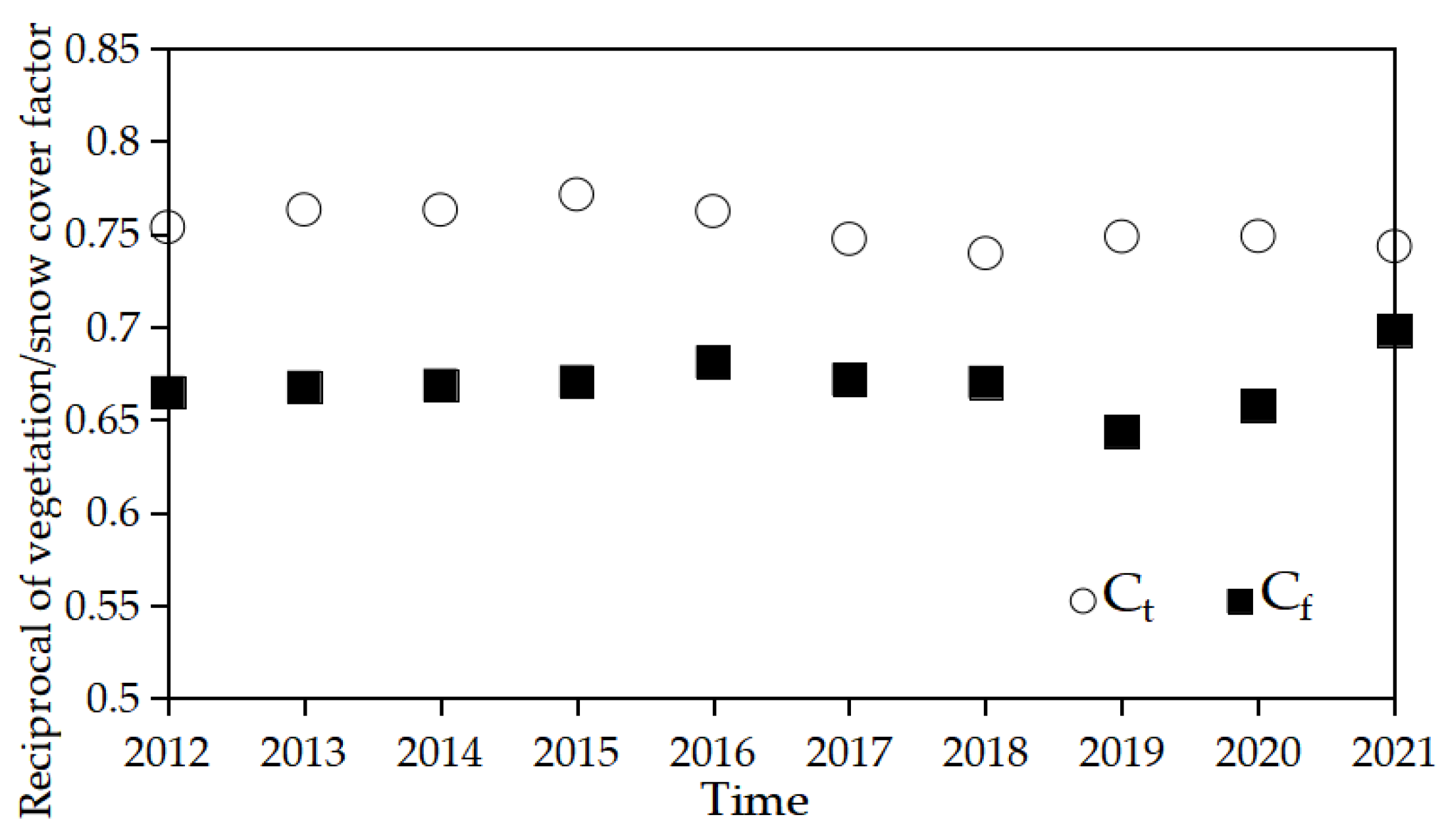
3.1.2. Reciprocals of Vegetation and Snow Cover Factors (Ct and Cf)

Figure 5 shows the reciprocals of vegetation and snow cover factors, Ct and Cf, for each year from 2012 to 2021, calculated from the FVC and FSC values, respectively. It can be seen that vegetation and snow cover throughout the study area generally remained at low levels throughout this period, indicating little variation.

3.1.3. PE Factors (pet and pef)

Figure 6 displays the PE factors for each year as points with each interpolation curve. The pet factor is larger than pef throughout the period, but only in 2013 is pef larger, most likely due to reduced precipitation.

3.1.4. Corrected Soil Thermal Conductivities (St and Sf)

Figure 7 compares the box plots of the soil thermal conductivity between the validation values (64 samples for each period) and the values calculated with the PE factors for the thawing and freezing periods, where each box indicates ± 3σ. It can be seen that the validation and calculated values correlate well—95.7% and 96.3% of the calculated values met the three sigma criteria of the validation values in the thawing and freezing periods, respectively. Because the maximum value of the calculated values is close to the soil thermal conductivity under the net moisture content state after adding the PE factor, and the maximum value of the validation values is essentially the soil thermal conductivity under the saturated moisture content state, the maximum value of the calculated values is smaller than that of the validation values.

3.2. Application and Evaluation of TLZ Model

3.2.1. Permafrost Classification Maps with Four Classes

Figure 8 shows permafrost distributions classified into four classes (permafrost, transitional permafrost, seasonal permafrost, and short-term/non-permafrost) for each year from 2012 to 2021 using the modified TTOP values. Figure 9 shows the total count of pixels for each class for each year. It can be seen that permafrost areas fluctuate and decrease year by year and change to transitional permafrost. It can be also seen that both seasonal permafrost areas, and short-term/non-permafrost areas are stable during this period, but the latter tend to transform into the former.

3.2.2. Statistics of LST Maps

Figure 10 displays the maximum, minimum and mean of the LST maps obtained for each year from MODIS LST products. The LST tends to increase throughout the period, and this is especially evident in the maximum and minimum values. This can be partially attributed to global warming as well as effects associated with changes in vegetation and snow cover.

3.2.3. Mean Subsurface Temperatures at Different Depths

Figure 11 demonstrates the mean subsurface temperatures at the depths of 10, 20, 30, 40, 50 and 60 cm from 2012 to 2021 by the TLZ model, as a function of time. Figure 12 shows those values for 2012, which indicates that the zero-curtain effect was seen at the depths of 30, 50, and 60 cm below ground; however, this effect was not seen at 40 cm depth due to a lack of data. As shown in Figure 12, the subsurface temperatures at different depths in the thawing period (early April to mid-June) intersect the zero line for a brief period lasting no longer than 1 week; therefore, the zero-curtain effect in the thawing period cannot easily be used as a measure of the existence and stability of permafrost. On the other hand, the zero-curtain effect in the freezing period (mid-October to mid-November) is maintained for a longer period (about 3 or 4 weeks) and can be used as a measure to determine the existence and stability of permafrost.

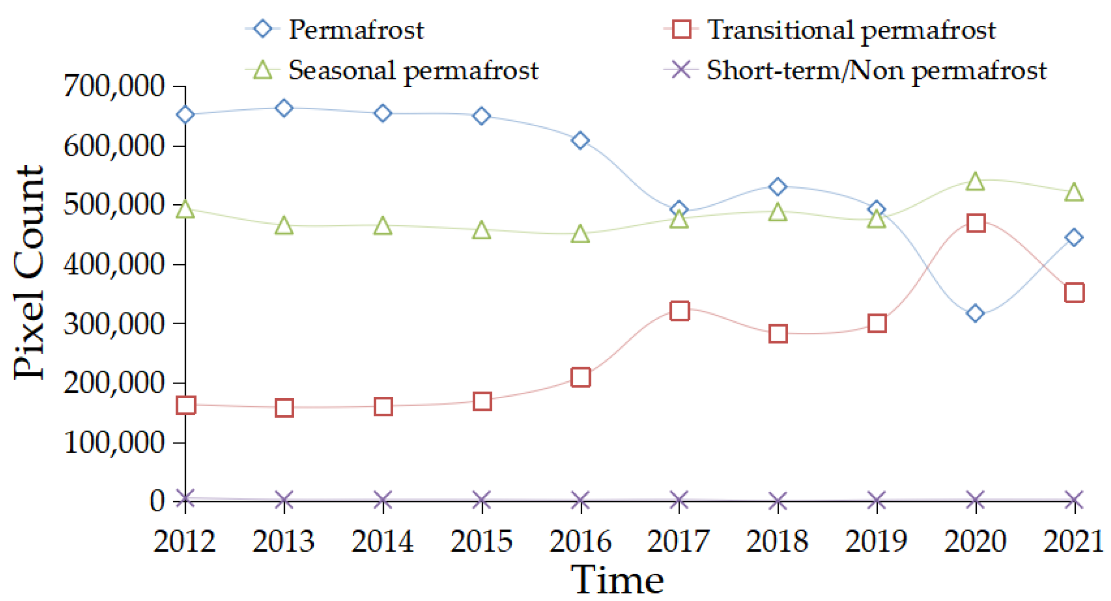
3.2.4. Permafrost Classification Maps with Seven Classes

Figure 13 shows permafrost distributions classified into seven classes (extremely stable, very stable, ordinary stable, unstable, transitional, seasonal, and short-term/non-permafrost), obtained by combining the TLZ model with the results of Figure 8. Figure 14 displays the total pixel count of each permafrost type as a function of time. From these figures, we can conclude the following.
  • Extremely and very stable classes slightly decreased during the study period. These decreases were mainly caused by changes from extremely to very stable classes, and very to ordinary stable classes, respectively.
  • Transitional class clearly increased in the period due to changes from ordinary stable and unstable classes.
  • Seasonal and short-term/non-permafrost classes did not show a significant change during the study period, while the former shows a somewhat large increase between 2019 and 2020.

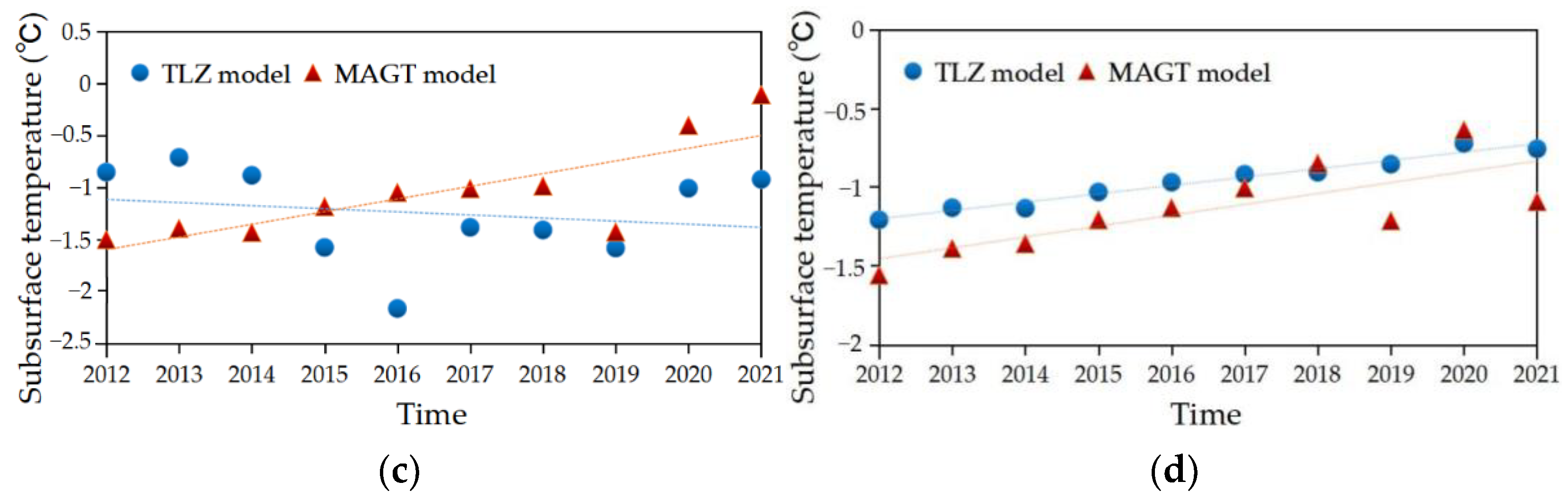
3.2.5. Comparison with the MAGT Model

Figure 15 shows daily mean subsurface temperatures among 27 CMDC stations at 30, 50, 60, and 300 cm depths for the period from 2012 to 2021. In Figure 16, the MAGT values calculated from these data are compared with the annual means of subsurface temperatures estimated by the TLZ model in the period for each depth. Table 2 gives the standard error, mean absolute error, and RMSE of subsurface temperatures by the TLZ model with reference to the MAGT-based values for four depths. Their mean values are 0.25, 0.27, and 0.19, respectively, all much smaller than 1, indicating that the TLZ model results of this study are highly accurate.

4. Discussion

Permafrost analysis requires data and a model that are both valid and accurate. In order to perform more valid and accurate permafrost analysis in the Qinghai–Tibetan Plateau region, we first proposed a modified TTOP model incorporating the PE factors and then proposed a TLZ model to classify permafrost in detail based on zero-curtain effects by combining the modified TTOP with LST data.
In the permafrost mapping of the study area with the modified TTOP model, it was found that the main change in the permafrost type occurred between permafrost and transitional permafrost, and seasonal permafrost increased in the period of 2012–2021. Overall, the permafrost trend in the period shows a more pronounced degradation trend, but permafrost shows two small rebounds in 2018 and 2021. As a result of analyzing the climatic conditions in 2018 and 2021, the greenhouse effect continued in the study area and the mean air-temperature still increased in both years, but there were fewer extreme weather events. The mean values of precipitation and snowfall were relatively stable, and the vegetation had developed to a certain extent, which may be the reason for the delayed degradation of permafrost in both years. The mean value of TTOP in the freezing period was higher than that in the thawing period because the active layer releases heat to the outside during the freezing period, increasing the temperature at the contact between the active layer and the permafrost layer.
In the zero-curtain analysis based on the TLZ model, it was found that the zero-curtain effect only exists in the freezing period of the active layer (mid-October to mid-November in this study), and the existence and stability of permafrost can only be investigated during the zero-curtain effect in the freezing period. These results are the same as those of a previous study by Gillespie et al. The difference between our study and the study of Gillespie et al. [48] is the depth at which the zero-curtain effect occurs. Our results, as shown in Figure 12, reveal that the zero-curtain effect occurs at 30, 50, and 60 cm, while in the previous study by Gillespie et al., the zero-curtain effect mainly occurred at 15, 25, and 30 cm. The most likely causes of this difference are the differences in soil properties between our study area (Qinghai–Tibetan Plateau region in Asia) and their study area (Chilean region in South America) and differences in how zero-curtain effects are determined. Gillespie et al. judged the zero-curtain effect based only on LST, but we determined the zero-curtain effect based on the combination of LST and TTOP using the TLZ hierarchical algorithm. Because the zero-curtain discrimination is based on LST in Gillespie et al.’s study, they verified zero-curtain occurrence using LST with a subsurface temperature at 2 cm depth at three subsurface temperature observation sites, which indirectly proved the accuracy of zero-curtain speculation [48]. In contrast, in this study, the MAGT model was constructed to directly validate the subsurface temperature at the depth of zero-curtain occurrence using 27 actual measured subsurface temperature data for comparison. There are differences in the validation techniques between the two studies, and because Gillespie et al. did not provide specific accuracy validation values in their previous study, we cannot compare them using specific values such as RMSE to those in this study. However, in general, the direct validation method is more accurate than the indirect validation method. We also compared the error results at different depths with those of Zhao et al., who also studied a zero-curtain effect to detect permafrost changes in the Qinghai–Tibetan Plateau region [51]. Their mean errors at 5, 10, 40, 105, and 245 cm exceeded 0.4 °C, indicating that the mean errors of the TLZ model at different depths are smaller than the conventional zero-curtain model.
In permafrost mapping based on the TLZ model, the study area was classified to seven permafrost classes for each year in the period 2012–2021. In this period, extremely and very stable classes slightly decreased, and transitional class significantly increased, while seasonal and short-term/non-permafrost classes did not show a significant change. These changes can be investigated by analyzing conversions between different types. Particularly, the decreases in extremely and very stable classes were mainly caused by changes from extremely to very stable classes, and very to ordinary stable classes, respectively, and the increase in transitional class was mainly due to changes from ordinary stable and unstable classes. These changes indicate the overall degradation of permafrost in the study area, probably due to the recent onset of global warming. In 2020, the results show a somewhat different tendency, most likely due to the frequent occurrence of several extreme weather events in 2020. This indicates that the frequency of extreme weather phenomena, as well as the increase in air temperature, may affect permafrost stability.
In the validation study based on the MAGT model, it was shown that the average of RMSE between the MAGT-based and the TLZ-based values was 0.19 °C. Ni et al. reported a mean RMSE of 0.53 °C in 2021 when using the TTOP model and the MAGT model for the active layer (0–2.99 m) of the Qinghai–Tibetan Plateau [44]. Ran et al. (2022) reported a mean RMSE of 0.93 °C when analyzing the active layer (2.35 m) of the Qinghai–Tibetan Plateau using the TTOP model and the MAGT model [45]. Yin et al. (2021) reported a mean RMSE of 0.5 °C when analyzing the active layer (0.69–4.32 m) of the Qinghai–Tibetan Plateau using the TTOP model and the MAGT model RMSE [46]. Compared to their study, our RMSE value of 0.19 °C is small enough, indicating that the TLZ model is higher in accuracy than conventional TTOP models. It should be noted that even after removing the effect of vegetation and snow, there is still some difference between LST and 0 cm temperature, and a more reasonable method to convert the former to the latter should be considered in future studies.

5. Conclusions

In this study, a TLZ model was proposed to analyze the zero-curtain effect in permafrost, with LST as the upper-limit temperature and TTOP as the lower-limit temperature. Here, the formula for calculating TTOP was modified to include new PE factors to take into account the effect of soil water content. Compared with the conventional TTOP-based models, the TLZ model is expected to better reflect the state of the active layer using LST instead of the air temperature. Compared with the LST–zero-curtain model proposed by Gillespie et al., the TLZ model is expected to more realistically evaluate the zero-curtain effect based on the lower-limit temperature of the active layer of permafrost with a curvilinear variation. Using this model, we evaluated permafrost distribution and temporal change at large, medium, and small scales in the central–eastern area of the Tibetan Plateau from 2012 to 2021, and validated the results using the MAGT model, indicating the superiority of the TLZ model in comparison with the conventional TTOP and LST–zero-curtain models. The TLZ model can not only judge the existence area of permafrost in a large or medium scale, but also conducted detailed small-scale analyses of stability, periodic change patterns, permafrost type transition, and degradation prediction. The TLZ model is a new direction for permafrost mapping and permafrost analysis studies at different scales and requires a higher accuracy. These features of the TLZ model will be significant advantages over conventional methods for permafrost analysis.

Author Contributions

Conceptualization, Z.Z. and H.T.; methodology, Z.Z.; software, Z.Z.; validation, Z.Z.; formal analysis, Z.Z.; investigation, Z.Z.; resources, Z.Z.; data curation, Z.Z.; writing—original draft preparation, Z.Z.; writing—review and editing, H.T.; visualization, Z.Z.; supervision, H.T.; project administration, H.T.; funding acquisition, H.T. All authors have read and agreed to the published version of the manuscript.

Funding

This research received no external funding.

Institutional Review Board Statement

Not applicable.

Informed Consent Statement

Not applicable.

Data Availability Statement

Not applicable.

Conflicts of Interest

The authors declare no conflict of interest.

References

  1. Ma, W.; Cheng, G.; Wu, Q. Construction on permafrost foundations: Lessons learned from the Qinghai–Tibet railroad. Cold Reg. Sci. Technol. 2009, 59, 3–11. [Google Scholar]
  2. Harris, C.; Davies, M.C.R.; Etzelmüller, B. The assessment of potential geotechnical hazards associated with mountain permafrost in a warming global climate. Permafr. Periglac. Process. 2001, 12, 145–156. [Google Scholar] [CrossRef]
  3. Gruber, S. Derivation and analysis of a high-resolution estimate of global permafrost zonation. Cryosphere 2012, 6, 221–233. [Google Scholar] [CrossRef] [Green Version]
  4. Kimball, J.S.; McDonald, K.C.; Keyser, A.R.; Frolking, S.; Running, S.W. Application of the NASA Scatterometer (NSCAT) for Determining the Daily Frozen and Nonfrozen Landscape of Alaska. Remote Sens. Environ. 2001, 75, 113–126. [Google Scholar] [CrossRef]
  5. Briggs, M.A.; Walvoord, M.A.; McKenzie, J.M.; Voss, C.I.; Day-Lewis, F.D.; Lane, J.W. New permafrost is forming around shrinking Arctic lakes, but will it last? Geophys. Res. Lett. 2014, 41, 1585–1592. [Google Scholar] [CrossRef]
  6. Dobiński, W. Permafrost active layer. Earth-Sci. Rev. 2020, 208, 103301. [Google Scholar] [CrossRef]
  7. Mekonnen, Z.A.; Riley, W.J.; Grant, R.F.; Romanovsky, V.E. Changes in precipitation and air temperature contribute comparably to permafrost degradation in a warmer climate. Environ. Res. Lett. 2021, 16, 024008. [Google Scholar] [CrossRef]
  8. Romanovsky, V.E.; Osterkamp, T.E. Thawing of the Active Layer on the Coastal Plain of the Alaskan Arctic. Permafr. Periglac. Process. 1998, 8, 1–22. [Google Scholar] [CrossRef]
  9. Zhang, T.; Frauenfeld, O.W.; Serreze, M.C.; Etringer, A.; Oelke, C.; McCreight, J.L.; Barry, R.; Gilichinsky, D.; Yang, D.; Ye, H.; et al. Spatial and temporal variability in active layer thickness over the Russian Arctic drainage basin. J. Geophys. Res. 2005, 110, D16101. [Google Scholar] [CrossRef]
  10. Hinkel, K.M.; Outcalt, S.I.; Taylor, A.E. Seasonal patterns of coupled flow in the active layer at three sites in northwest North America. Can. J. Earth Sci. 1997, 34, 667–678. [Google Scholar] [CrossRef]
  11. Luo, D.; Jin, H.; Marchenko, S.S.; Romanovsky, V.E. Difference between near-surface air, land surface and ground surface temperatures and their influences on the frozen ground on the Qinghai-Tibet Plateau. Geoderma 2018, 312, 74–85. [Google Scholar] [CrossRef]
  12. Hachem, S.; Allard, M.; Duguay, C. Using the MODIS land surface temperature product for mapping permafrost: An application to northern Québec and Labrador, Canada. Permafr. Periglac. Process. 2009, 20, 407–416. [Google Scholar] [CrossRef]
  13. Zou, D.; Zhao, L.; Sheng, Y.; Chen, J.; Hu, G.; Wu, T.; Wu, J.; Xie, C.; Wu, X.; Pang, Q.; et al. A new map of permafrost distribution on the Tibetan Plateau. Cryosphere 2017, 11, 2527–2542. [Google Scholar] [CrossRef] [Green Version]
  14. Shen, X.; Liu, B.; Jiang, M.; Lu, X. Marshland loss warms local land surface temperature in China. Geophys. Res. Lett. 2020, 47, e2020GL087648. [Google Scholar] [CrossRef] [Green Version]
  15. Qin, Y.; Wu, T.; Zhao, L.; Wu, X.; Li, R.; Xie, C.; Pang, Q.; Hu, G.; Qiao, Y.; Zhao, G.; et al. Numerical modeling of the active layer thickness and permafrost thermal state across Qinghai-Tibetan Plateau. J. Geophys. Res. Atmos. 2017, 122, 11604–11620. [Google Scholar] [CrossRef]
  16. Sun, Z.; Zhao, L.; Hu, G.; Qiao, Y.; Du, E.; Zou, D.; Xie, C. Modeling permafrost changes on the Qinghai-Tibetan Plateau from 1966 to 2100: A case study from two boreholes along the Qinghai-Tibet engineering corridor. Permafr. Periglac. Process. 2020, 31, 156–171. [Google Scholar] [CrossRef]
  17. Peng, X.; Zhang, T.; Frauenfeld, O.W.; Wang, K.; Luo, D.; Cao, B.; Su, H.; Jin, H.; Wu, Q. Spatiotemporal changes in active layer thickness under contemporary and projected climate in the Northern Hemisphere. J. Clim. 2018, 31, 251–266. [Google Scholar] [CrossRef]
  18. Zhao, L.; Zou, D.; Hu, G.; Du, E.; Pang, Q.; Xiao, Y.; Li, R.; Sheng, Y.; Wu, X.; Sun, Z.; et al. Changing climate and the permafrost environment on the Qinghai-Tibet (Xizang) Plateau. Permafr. Periglac. Process. 2020, 31, 396–405. [Google Scholar] [CrossRef]
  19. Wei, Y.; Lu, H.; Wang, J.; Wang, X.; Sun, J. Dual Influence of Climate Change and Anthropogenic Activities on the Spatiotemporal Vegetation Dynamics Over the Qinghai-Tibetan Plateau From 1981 to 2015. Earth’s Future 2022, 10, e2021EF002566. [Google Scholar] [CrossRef]
  20. Liu, Y.; Fang, P.; Guo, B.; Ji, M.; Liu, P.; Mao, G.; Xu, B.; Kang, S.; Liu, J. A comprehensive dataset of microbial abundance, dissolved organic carbon, and nitrogen in Tibetan Plateau glaciers. Earth Syst. Sci. Data 2022, 14, 2303–2314. [Google Scholar] [CrossRef]
  21. Mu, C.C.; Abbott, B.W.; Wu, X.D.; Zhao, Q.; Wang, H.J.; Su, H.; Wang, S.F.; Gao, T.G.; Guo, H.; Peng, X.Q.; et al. Thaw depth determines dissolved organic carbon concentration and biodegradability on the northern Qinghai-Tibetan Plateau. Geophys. Res. Lett. 2017, 44, 9389–9399. [Google Scholar] [CrossRef]
  22. McGuire, A.D.; Koven, C.; Lawrence, D.M.; Clein, J.S.; Xia, J.; Beer, C.; Burke, E.; Chen, G.; Chen, X.; Delire, C.; et al. Variability in the sensitivity among model simulations of permafrost and carbon dynamics in the permafrost region between 1960 and 2009. Glob. Biogeochem. Cycles 2016, 30, 1015–1037. [Google Scholar] [CrossRef] [Green Version]
  23. Nieberding, F.; Wille, C.; Fratini, G.; Asmussen, M.O.; Wang, Y.; Ma, Y.; Sachs, T. A long-term (2005–2019) eddy covariance data set of CO2 and H2O fluxes from the Tibetan alpine steppe. Earth Syst. Sci. Data 2020, 12, 2705–2724. [Google Scholar] [CrossRef]
  24. Wang, Y.; Wang, L.; Li, X.; Zhou, J.; Hu, Z. An integration of gauge, satellite, and reanalysis precipitation datasets for the largest river basin of the Tibetan Plateau. Earth Syst. Sci. Data 2020, 12, 1789–1803. [Google Scholar] [CrossRef]
  25. Huang, Z.; Zhong, L.; Ma, Y.; Fu, Y. Development and evaluation of spectral nudging strategy for the simulation of summer precipitation over the Tibetan Plateau using WRF (v4.0). Geosci. Model Dev. 2021, 14, 2827–2841. [Google Scholar] [CrossRef]
  26. Zhang, G.; Nan, Z.; Wu, X.; Ji, H.; Zhao, S. The role of winter warming in permafrost change over the Qinghai-Tibet Plateau. Geophys. Res. Lett. 2019, 46, 11261–11269. [Google Scholar] [CrossRef] [Green Version]
  27. Nikiforoff, C. The perpetually frozen subsoil of siberia. Soil Sci. 1928, 26, 61–82. [Google Scholar] [CrossRef]
  28. Stefan, J. Ueber die Theorie der Eisbildung, insbesondere über die Eisbildung im Polarmeere. Ann. Phys. 1891, 278, 269–286. [Google Scholar] [CrossRef] [Green Version]
  29. Berggren, W.P. Prediction of temperature-distribution in frozen soils. Eos Trans. Am. Geophys. Union 1943, 24, 71–77. [Google Scholar] [CrossRef]
  30. Nelson, F.E.; Outcalt, S.I. A Computational Method for Prediction and Regionalization of Permafrost. Arct. Alp. Res. 1987, 19, 279–288. [Google Scholar] [CrossRef]
  31. Anisimov, O.A.; Nelson, F.E. Permafrost distribution in the Northern Hemisphere under scenarios of climatic change. Glob. Planet. Chang. 1996, 14, 59–72. [Google Scholar] [CrossRef]
  32. Nelson, F.E.; Shiklomanov, N.I.; Mueller, G.R.; Hinkel, K.M.; Walker, D.A.; Bockheim, J.G. Estimating Active-Layer Thickness over a Large Region: Kuparuk River Basin, Alaska, USA. Arct. Alp. Res. 1997, 29, 367–378. [Google Scholar] [CrossRef]
  33. Nelson, F.E.; Anisimov, O.A.; Shiklomanov, N.I. Climate Change and Hazard Zonation in the Circum-Arctic Permafrost Regions. Nat. Hazards 2002, 26, 203–225. [Google Scholar] [CrossRef]
  34. Nelson, F.E.; Shiklomanov, N.I.; Hinkel, K.M.; Christiansen, H.H. The Circumpolar Active Layer Monitoring (CALM) Workshop and THE CALM II Program. Polar Geogr. 2004, 28, 253–266. [Google Scholar] [CrossRef]
  35. Kudryavtsev, V.A.; Garagulya, L.S.; Kondratyeva, K.A.; Melamed, V.G. Fundamentals of Frost Forecasting in Geological Engineering Investigations; Moscow State University Press: Nakuka, Moscow, 1974; Volume 431. [Google Scholar]
  36. Shiklomanov, N.I.; Nelson, F.E. Analytic representation of the active layer thickness field, Kuparuk River Basin, Alaska. Ecol. Model. 1999, 123, 105–125. [Google Scholar] [CrossRef]
  37. Nan, Z.; Li, S.; Cheng, G. Prediction of permafrost distribution on the Qinghai-Tibet Plateau in the next 50 and 100 years. Sci. China Ser. D-Earth Sci. 2005, 48, 797–804. [Google Scholar] [CrossRef]
  38. Aalto, J.; Karjalainen, O.; Hjort, J.; Luoto, M. Statistical forecasting of current and future circum-Arctic ground temperatures and active layer thickness. Geophys. Res. Lett. 2018, 45, 4889–4898. [Google Scholar] [CrossRef] [Green Version]
  39. Smith, M.W.; Riseborough, D.W. Permafrost monitoring and detection of climate change. Permafr. Periglac. Process. 1996, 7, 301–309. [Google Scholar] [CrossRef]
  40. Riseborough, D.W. The mean annual temperature at the top of permafrost, the TTOP model, and the effect of unfrozen water. Permafr. Periglac. Process. 2002, 13, 137–143. [Google Scholar] [CrossRef]
  41. Garibaldi, M.C.; Bonnaventure, P.P.; Lamoureux, S.F. Utilizing the TTOP model to understand spatial permafrost temperature variability in a High Arctic landscape, Cape Bounty, Nunavut, Canada. Permafr. Periglac. Process. 2021, 32, 19–34. [Google Scholar] [CrossRef]
  42. Juliussen, H.; Humlum, O. Towards a TTOP ground temperature model for mountainous terrain in central-eastern Norway. Permafr. Periglac. Process. 2007, 18, 161–184. [Google Scholar] [CrossRef]
  43. Zhang, Y.; Zang, S.; Li, M.; Shen, X.; Lin, Y. Spatial Distribution of Permafrost in the Xing’an Mountains of Northeast China from 2001 to 2018. Land 2021, 10, 1127. [Google Scholar] [CrossRef]
  44. Ni, J.; Wu, T.; Zhu, X.; Hu, G.; Zou, D.; Wu, X.; Li, R.; Xie, C.; Qiao, Y.; Pang, Q.; et al. Simulation of the Present and Future Projection of Permafrost on the Qinghai-Tibet Plateau with Statistical and Machine Learning Models. JGR Atmos. 2021, 126, e2020JD033402. [Google Scholar] [CrossRef]
  45. Ran, Y.; Li, X.; Che, T.; Wang, B.; Cheng, G. Current state and past changes in frozen ground at the Third Pole: A research synthesis. Adv. Clim. Chang. Res. 2022, 13, 632–641. [Google Scholar] [CrossRef]
  46. Yin, G.; Niu, F.; Lin, Z.; Luo, J.; Liu, M. Data-driven spatiotemporal projections of shallow permafrost based on CMIP6 across the Qinghai–Tibet Plateau at 1 km2 scale. Adv. Clim. Chang. Res. 2021, 12, 814–827. [Google Scholar] [CrossRef]
  47. Obu, J.; Westermann, S.; Bartsch, A.; Berdnikov, N.; Christiansen, H.H.; Dashtseren, A.; Delaloye, R.; Elberling, B.; Etzelmüller, B.; Kholodov, A.; et al. Northern Hemisphere permafrost map based on TTOP modelling for 2000–2016 at 1 km2 scale. Earth-Sci. Rev. 2019, 193, 299–316. [Google Scholar] [CrossRef]
  48. Batbaatar, J.; Gillespie, A.R.; Sletten, R.S.; Mushkin, A.; Amit, R.; Trombotto Liaudat, D.; Liu, L.; Petrie, G. Toward the Detection of Permafrost Using Land-Surface Temperature Mapping. Remote Sens. 2020, 12, 695. [Google Scholar] [CrossRef] [Green Version]
  49. Outcalt, S.I.; Nelson, F.E.; Hinkel, K.M. The zero-curtain effect: Heat and mass transfer across an isothermal region in freezing soil. Water Resour. Res. 1990, 26, 1509–1516. [Google Scholar]
  50. Gillespie, A.R.; Batbaatar, J.; Sletten, R.S.; Trombotto, D.; O’Neal, M.; Hanson, B.; Mushkin, A. Monitoring and mapping soil ice/water phase transitions in arid regions. In Geological Society of America Abstracts with Programs; Geological Society of America: Boulder, CO, USA, 2017. [Google Scholar]
  51. Zhao, Y.; Nan, Z.; Ji, H.; Zhao, L. Convective heat transfer of spring meltwater accelerates active layer phase change in Tibet permafrost areas. Cryosphere 2022, 16, 825–849. [Google Scholar] [CrossRef]
  52. Wang, C.; Zhang, Z.; Zhang, H.; Zhang, B.; Tang, Y.; Wu, Q. Active Layer Thickness Retrieval of Qinghai–Tibet Permafrost Using the TerraSAR-X InSAR Technique. IEEE J. Sel. Top. Appl. Earth Obs. Remote Sens. 2018, 11, 4403–4413. [Google Scholar] [CrossRef]
  53. Ran, Y.; Li, X.; Cheng, G.; Zhang, T.; Wu, Q.; Jin, H.; Jin, R. Distribution of Permafrost in China: An Overview of Existing Permafrost Maps. Permafr. Periglac. Process. 2012, 23, 322–333. [Google Scholar] [CrossRef]
  54. Zhang, G.; Nan, Z.; Hu, N.; Yin, Z.; Zhao, L.; Cheng, G.; Mu, C. Qinghai-Tibet Plateau Permafrost at Risk in the Late 21st Century. Earth’s Future 2022, 10, e2022EF002652. [Google Scholar] [CrossRef]
  55. Feng, S.; Tang, M.; Wang, D. New evidence for the Qinghai-Xizang(Tibet)Plateau as a pilot region of climatic fluctuation in China. Chin. Sci. Bull. 1998, 43, 1745–1749. [Google Scholar] [CrossRef]
  56. Peng, J.; Liu, Z.; Liu, Y.; Wu, J.; Han, Y. Trend analysis of vegetation dynamics in Qinghai–Tibet Plateau using Hurst Exponent. Ecol. Indic. 2012, 14, 28–39. [Google Scholar] [CrossRef]
  57. Wang, Z.; Fan, H.; Wang, D.; Xing, T.; Wang, D.; Guo, Q.; Xiu, L. Spatial Pattern of Highway Transport Dominance in Qinghai–Tibet Plateau at the County Scale. ISPRS Int. J. Geo-Inf. 2021, 10, 304. [Google Scholar] [CrossRef]
  58. Johansen, O. Thermal Conductivity of Soils. Ph.D. Thesis, University of Trondheim, Trondheim, Norway, 1975. (Draft English Translation 637, US Army Corps of Engineers, Cold Regions Research and Engineering Laboratory, Hanover, New Hampshire ed.). [Google Scholar]
  59. Walvoord, M.A.; Kurylyk, B.L. Hydrologic Impacts of Thawing Permafrost—A Review. Vadose Zone J. 2016, 15, vzj2016.01.0010. [Google Scholar] [CrossRef] [Green Version]
  60. Kukkonen, I.T.; Suhonen, E.; Ezhova, E.; Lappalainen, H.; Gennadinik, V.; Ponomareva, O.; Gravis, A.; Miles, V.; Kulmala, M.; Melnikov, V.; et al. Observations and modelling of ground temperature evolution in the discontinuous permafrost zone in Nadym, north-west Siberia. Permafr. Periglac. Process. 2020, 31, 264–280. [Google Scholar] [CrossRef]
  61. Donato, G.; Belongie, S. Approximate Thin Plate Spline Mappings. In Proceedings of the Computer Vision—ECCV 2002, Copenhagen, Denmark, 28–31 May 2002; Heyden, A., Sparr, G., Nielsen, M., Johansen, P., Eds.; Spring: Berlin/Heidelberg, Germany, 2002; Volume 2352, pp. 21–31. [Google Scholar]
  62. Deng, Z.; Lu, Z.; Wang, G.; Wang, D.; Ding, Z.; Zhao, H.; Xu, H.; Shi, Y.; Cheng, Z.; Zhao, X. Extraction of fractional vegetation cover in arid desert area based on Chinese GF-6 satellite. Open Geosci. 2021, 13, 416–430. [Google Scholar] [CrossRef]
  63. Jiang, L.; Pan, F.; Wang, G.; Pan, J.; Shi, J.; Zhang, C. MODIS Daily Cloud-Free Factional Snow Cover Data Set for Asian Water Tower Area (2000–2022); National Tibetan Plateau Data Center: Beijing, China, 2022. [Google Scholar]
  64. Tarnawski, V.R.; Momose, T.; McCombie, M.L.; Leong, W.H. Canadian field soils III. Thermal-conductivity data and modeling. Int. J. Thermophys. 2015, 36, 119–156. [Google Scholar] [CrossRef]
  65. McInnes, K.J. Thermal Conductivities of Soils from Dryland Wheat Regions of Eastern Washington. Master’s Thesis, Washington State University, Washington, DC, USA, 1981. [Google Scholar]
  66. Hopmans, J.W.; Dane, J.H. Thermal conductivity of two porous media as a function of water content, temperature, and density. Soil Sci. 1986, 142, 187–195. [Google Scholar] [CrossRef]
  67. Campbell, G.S.; Jungbauer, J.D., Jr.; Bidlake, W.R.; Hungerford, R.D. Predicting the effect of temperature on soil thermal conductivity. Soil Sci. 1994, 158, 307–313. [Google Scholar] [CrossRef]
  68. Côté, J.; Konrad, J.M. A generalized thermal conductivity model for soils and construction materials. Can. Geotech. J. 2005, 42, 443–458. [Google Scholar] [CrossRef]
  69. Kasubuchi, T.; Momose, T.; Tsuchiya, F.; Tarnawski, V.R. Normalized thermal conductivity model for three Japanese soils. Trans. Jpn. Soc. Irrig. Drain. Rural Eng. 2007, 75, 529–533. [Google Scholar]
  70. Lu, S.; Ren, T.; Gong, Y.; Horton, R. An improved model for predicting soil thermal conductivity from water content at room temperature. Soil Sci. Soc. Am. J. 2007, 71, 8–14. [Google Scholar] [CrossRef]
  71. Chen, S.X. Thermal conductivity of sands. Heat Mass Transf. 2008, 44, 1241–1246. [Google Scholar] [CrossRef]
  72. Tarnawski, V.R.; McCombie, M.L.; Leong, W.H.; Wagner, B.; Momose, T.; Schönenberger, J. Canadian field soils II. Modeling of quartz occurrence. Int. J. Thermophys. 2012, 33, 843–863. [Google Scholar] [CrossRef]
  73. McCombie, M.L.; Tarnawski, V.R.; Bovesecchi, G.; Coppa, P.; Leong, W.H. Thermal conductivity of pyroclastic soil (Pozzolana) from the environs of Rome. Int. J. Thermophys. 2017, 38, 21. [Google Scholar] [CrossRef]
Figure 1. Location of study area (blue polygon) and six subareas (A to F) in the Qinghai–Tibetan Plateau, China. Red asterisks indicate the locations of CMDC stations.
Remotesensing 14 06350 g001
Figure 2. Conceptual diagram of TLZ model.
Remotesensing 14 06350 g002
Figure 3. Daily mean air-temperature trends in the period from 2012 to 2021 in six groups A to F.
Remotesensing 14 06350 g003
Figure 4. Cumulative temperature factors, At and Af, in the period from 2012 to 2021.
Remotesensing 14 06350 g004
Figure 5. Reciprocals of vegetation and snow cover factors, Ct and Cf, for the period from 2012 to 2021.
Remotesensing 14 06350 g005
Figure 6. Temporal changes in PE factors (pet and pef) for the period from 2012 to 2021.
Remotesensing 14 06350 g006
Figure 7. Comparison of the box plots of the soil thermal conductivity between the validation values (64 samples for each period) and the values calculated with the PE factors for (a) the thawing period and (b) the freezing period. Box indicates ± 3σ.
Remotesensing 14 06350 g007
Figure 8. Permafrost distributions classified into four classes (permafrost, transitional permafrost, seasonal permafrost, and short-term/non-permafrost) for each year from 2012 to 2021.
Remotesensing 14 06350 g008
Figure 9. Total count of pixels for each class (permafrost, transitional permafrost, seasonal permafrost, and short-term/non-permafrost) for each year from 2012 to 2021.
Remotesensing 14 06350 g009
Figure 10. Maximum, minimum and mean of LST maps obtained for each year from MODIS LST products.
Remotesensing 14 06350 g010
Figure 11. Temporal changes in the mean subsurface temperatures at depths of 10, 20, 30, 40, 50 and 60 cm for the period from 2012 to 2021, obtained by the TLZ model.
Remotesensing 14 06350 g011
Figure 12. Temporal changes of the mean subsurface temperatures at the depths of 10, 20, 30, 40, 50 and 60 cm in 2012, obtained by the TLZ model.
Remotesensing 14 06350 g012
Figure 13. Permafrost distributions classified into seven classes (extremely stable, very stable, ordinary stable, unstable, transitional, seasonal, and short-term/non-permafrost) for each year from 2012 to 2021.
Remotesensing 14 06350 g013
Figure 14. Total count of pixels for each class (extremely stable, very stable, ordinary stable, unstable, transitional, seasonal, and short-term/non-permafrost) for each year from 2012 to 2021.
Remotesensing 14 06350 g014
Figure 15. Daily mean subsurface temperatures among 27 CMDC stations at 30, 50, 60, and 300 cm depths for the period from 2012 to 2021.
Remotesensing 14 06350 g015
Figure 16. Comparison of the MAGT values and the subsurface temperatures estimated by the TLZ model for the period 2012–2021 for depths of (a) 30 cm, (b) 50 cm, (c) 60 cm, and (d) 300 cm.
Remotesensing 14 06350 g016aRemotesensing 14 06350 g016b
Table 1. Thermal conductivities of typical soil types in Qinghai–Tibetan Plateau in thawing and freezing periods reported by Johansen (1975) [58]. Numbers in bold are the maximum and minimum values, except for organic matter, used in the analysis of this study.
Soil TypeDry Density (kg·m−3)st (W∙m−1∙K−1)sf (W∙m−1∙K−1)
Sloping soils14001.15–1.541.61–2.69
Lacustrine soil14751.21–1.621.82–2.74
Wind-deposited soil15001.39–1.601.63–2.47
Ice and water deposition15501.26–1.661.65–2.50
Alluvial soils16001.30–1.721.59–2.53
Moraine17501.41–1.981.68–2.92
Organic matter3000.521.7
Table 2. Standard error, mean absolute error, and RMSE of subsurface temperatures by the TLZ model for depths of 30, 50, 60, and 300 cm, with reference to MAGT-based values.
Depth (cm)Standard Error (°C)Mean Absolute Error (°C)RMSE (°C)
300.2790.2380.192
500.1580.2910.200
600.4780.3550.198
3000.0940.1890.165
Publisher’s Note: MDPI stays neutral with regard to jurisdictional claims in published maps and institutional affiliations.

