A Study on the Effect of Multispectral LiDAR Data on Automated Semantic Segmentation of 3D-Point Clouds

Abstract

Mobile mapping is an application field of ever-increasing relevance. Data of the surrounding environment is typically captured using combinations of LiDAR systems and cameras. The large amounts of measurement data are then processed and interpreted, which is often done automated using neural networks. For the evaluation the data of the LiDAR and the cameras needs to be fused, which requires a reliable calibration of the sensors. Segmentation solemnly on the LiDAR data drastically decreases the amount of data and makes the complex data fusion process obsolete but on the other hand often performs poorly due to the lack of information about the surface remission properties. The work at hand evaluates the effect of a novel multispectral LiDAR system on automated semantic segmentation of 3D-point clouds to overcome this downside. Besides the presentation of the multispectral LiDAR system and its implementation on a mobile mapping vehicle, the point cloud processing and the training of the CNN are described in detail. The results show a significant increase in the mIoU when using the additional information from the multispectral channel compared to just 3D and intensity information. The impact on the IoU was found to be strongly dependent on the class.

1. Introduction

Mobile mapping is widely used to monitor and document our environment, e.g., ref. [1]. This technique combines a large number of sensors (cameras, positioning systems, etc.) with moving platforms (cars, drones, vessels, etc.) to generate georeferenced data quickly and efficiently. Comparable sensor and data settings are used for autonomous driving as well. In any case, the environment must be described as quickly and reliably as possible. The generated data can be used for building information modeling (BIM). However, for an efficient use of these data for BIM, the semantics of the objects have to be identified additionally. According to the state-of-the-art, an assignment of the individual 2D-pixels or 3D-points to predefined object classes and a subsequent clustering of these pixels or points is performed. An example of such a processing sequence can be found in [2]; a comparison between traditional geometric approaches and state-of-the-art machine learning can be found in [3].

Previous work has attempted to generate semantics through the interpretation of images in 2D space, the additional use of 3D information, or the sole use of 3D point clouds. In general, it can be said that the amount and level of detail of the information directly correlates with the quality of the semantic interpretation. Thus, if the semantic classification or segmentation is based on one data channel only (for example distance data), the result will most likely be worse compared to a solution based on multi-channel data sets, e.g., distance data and color information. In the case of LiDAR (light detection and ranging) the number of information channels is usually limited to 3D information and the intensity. The intensity is often not calibrated for the distance of the object to the sensor which makes it difficult to use for the identification of surface textures. This can be remedied by measuring with multiple laser wavelengths, which is referred to as multispectral LiDAR [4].

Already by selecting an adequate second laser wavelength, it is possible to generate significant added value in the measurement data and thus identify or describe objects more reliably. In [5] the potential of a dual-wavelength laser scanning system for the estimation of the vegetation moisture content has been evaluated. The study demonstrates the potential of single-wavelength combination between near infrared (1063 nm) and mid-infrared (1545 nm) wavelengths. In [6] the design of a full-waveform multispectral LiDAR including a first demonstration of its applications in remote sensing has been published. The system has been implemented by using a supercontinuum laser sources. The prototype has been evaluated in a laboratory application (scanning a small tree) and has shown that the approach makes it possible to study the chlorophyll or water concentration in vegetation.

Most of the developed multispectral LiDAR systems or experiments have been focused on the monitoring of vegetation. A high reflectance in the near infrared spectral region (NIR) compared to the visible is the basis for the vegetation characterization, examples can be found in [7,8]. In [9] a LiDAR system for the simultaneous measurement of geometry, remission and surface moisture for tunnel inspections employing a unique combination of the laser wavelengths 1450 nm and 1320 nm has been presented.

The advantage of such multispectral data over conventional LiDAR data for automated classification processes could already be shown by several studies. Most of these studies are performed on airborne multispectral LiDAR data due to the availability of commercial systems like the Teledyne Optech Titan.

In [10] a significant improvement in correctly classified land cover areas by a PointNet++ based neural network was reported when using multispectral LiDAR data captured by the Optech Titan instead of using only single wavelength information. An approach using a Transformer based network on the same data also showed significantly better results when using multispectral instead of single wavelength data [11].

Since the data of airborne and terrestrial LiDAR systems has very different characteristics when it comes to point density, accuracy, etc. these findings might not be applicable to terrestrial LiDAR data or other methods might be necessary.

When it comes to terrestrial LiDAR, a study using multispectral LiDAR data from stationary systems for automated rock outcrop classification found that the results were comparable to automated classification on passive digital photography data [12]. Advantages of multispectral over conventional terrestrial LiDAR systems for automated classification have been reported previously by [13] for data captured by a stationary system in a lab environment.

However, terrestrial mobile mapping by means of a multispectral LiDAR system is not established yet and is still a field of ongoing research.

The motivation for the work at hand is to use a multispectral LiDAR system (based on the working principle, as previously published in [13]) for the terrestrial mobile mapping application under real-world conditions and to evaluate the advantage compared to conventional systems—especially if the data is interpreted by machine learning methods.

2. Materials and Methods

The multispectral laser scanner used to generate the data for this study was developed recently at Fraunhofer IPM. The working principle of the dual wavelength approach will only be explained briefly in this article. A more detailed explanation can be found in [13]. The laser scanner employs two separate lasers, one with a wavelength of 1450 nm, the other with 1320 nm, that are coaxial aligned and continuously sending out light, modulated in their amplitude with different frequencies.

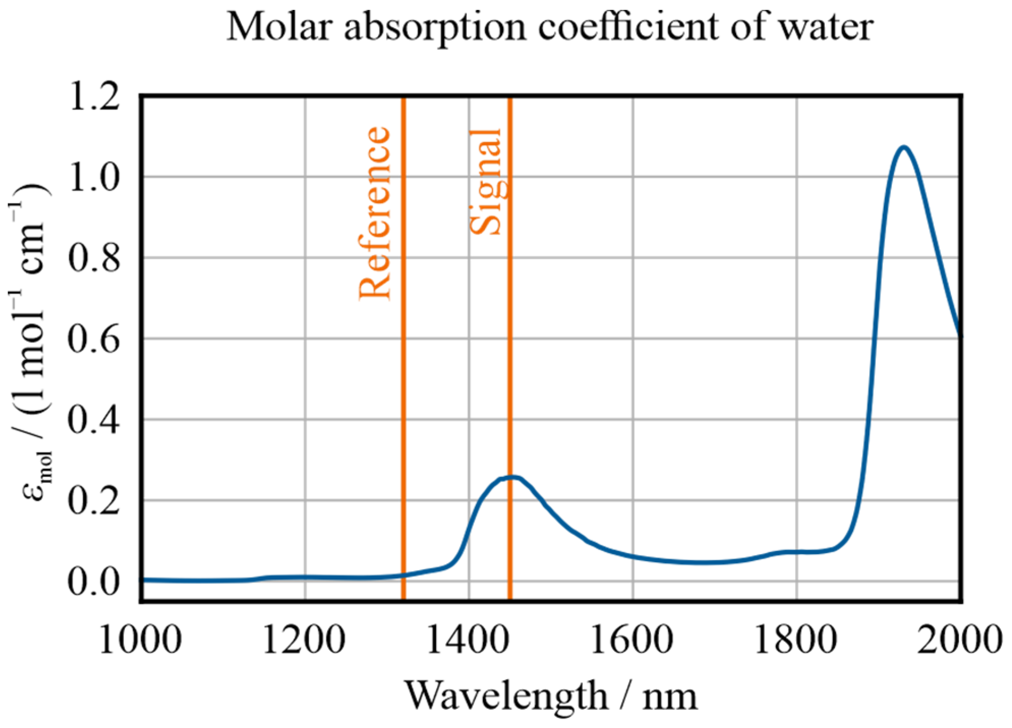
The 1450 nm wavelength was chosen because it is situated in the center of an absorption band of water, the 1320 nm are used as reference and were chosen as close as possible to 1450 nm without being affected by the absorption band. In Figure 1 the absorption coefficient of water in the near infrared region is shown with the two operating wavelengths of the laser scanner highlighted. Since the light from both lasers shares the same optical path, this is important to minimize the effect of chromatic aberration. The choice of wavelengths makes the scanner ideal for the detection of water on surfaces e.g., in tunnels, but also for materials with higher water content e.g., vegetation.

The backscattered light of both lasers is acquired simultaneously by an avalanche photodiode (APD). Through filtering the respective frequencies, their shares of the signal amplitude can be separated and compared. First the amplitudes are normalized to the re-turn signal of a target with approximately 90% reflectivity for distances from 1 to 10 m. Similarly, to the Normalized Difference Vegetation Index (NDVI), which is commonly used in satellite-based imaging to identify surfaces containing vegetation, a differential absorption value (DAV) is calculated and added to each measurement point of the laser scanner data.

$$DAV=\frac{I_{1320}-I_{1450}}{I_{1320}+I_{1450}}$$

Typically, dry surfaces show a differential absorption value around 0 and the values of wet surfaces or green vegetation are around 0.5. The standard deviation of the parameter is approximately 0.06. The main contribution to the standard deviation comes from intensity variations due to speckle that differ for the two wavelengths.

The measurement technique has been implemented into a robust profile scanner for mobile mapping with a 350° scanning angle, rotation frequency of up to 200 Hz and a measurement rate of 2 MHz [15].

To evaluate the advantage of the additional measurement channel in mobile mapping applications, real-world measurement data was generated by mounting the LiDAR system to a car and driving through residential areas.

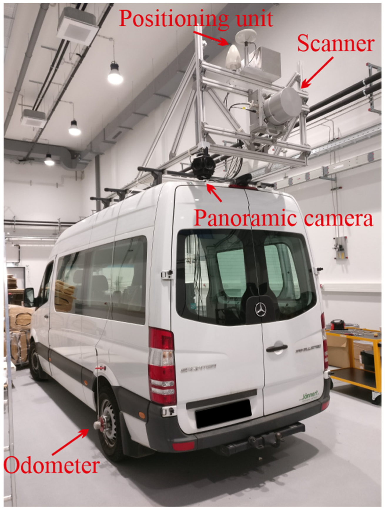
The configuration of the measurement vehicle included the LiDAR system, the positioning unit, a time server and a panoramic camera. The positioning unit generates a precise trajectory that is stored on a USB stick for later postprocessing of the point cloud. The NTP time server is used to synchronize the timestamps of the laser scanner data and the trajectory. The laser scanner is mounted with its scanning plane perpendicular to the driving direction, generating 200 profiles per second with 10,000 measurement points each. The distance between two profiles depends on the driving speed which was typically around 30 km/h in the residential areas which approximately leads to a profile every 4 cm. The laser scanner can capture data points well above 20 m on targets with a reflectivity above 90% but the quality of points with low reflectivity strongly degrades. For that reason, the maximum measurement distance for the evaluation via neural network was limited to 15 m. The mobile mapping vehicle is shown in Figure 2.

The measurement route covered various residential areas in and around Freiburg (Germany) to capture as heterogenous data as possible.

As a first step of postprocessing the trajectory was corrected.

The point clouds were calculated using the trajectory, the scanner data, and the calibrated lever arm between the origins of the coordinate systems of positioning unit and the scanner. The resulting point clouds contain georeferenced 3D data with remission and differential absorption value. The distance dependency of the intensity was calibrated so that the object remission could be derived from it. This was done by taking reference measurements on a calibrated measurement range from 0.5 m to 10 m in steps of 5 cm for targets with reflectivity of approximately 90%, 70%, 30% and 10%. From these measurements a lookup table was created with which the nonlinearity of the detector is corrected, and the intensity of the scanner is normed to the amount measured on a target with 90% reflectivity in the same distance.

The goal was to see whether the differential absorption value can have a significant impact on object recognition of a neural network in 3D-point clouds. The following classes, that are of relevance in mobile mapping, were chosen to evaluate the effect of multispectral information: leaf tree, pine tree, vegetation, grass, road, building and car. Every data point that did not belong to any of the classes was marked as unlabeled. 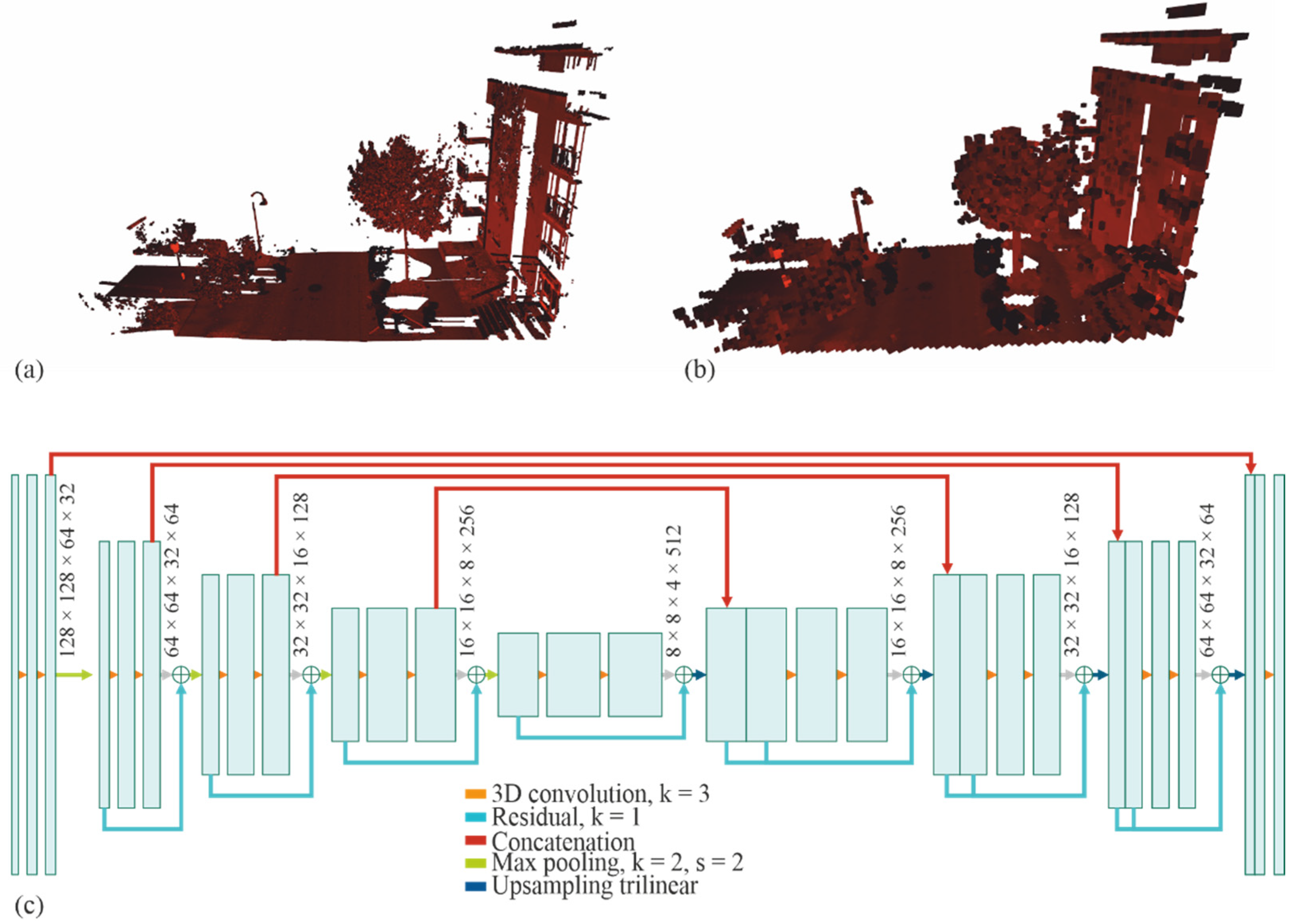The labeling was done manually using the open-source software CloudCompare [16]. In total 3 km of data of residential areas were labeled. The labeled point cloud was split into sections of 10 m length to reduce computation time of the network. An exemplary 30 m section of the point cloud is shown in Figure 3. Here (a) shows the point cloud with an intensity-based greyscale coloring and (b) shows the point cloud colored using the DAV.

Since the objects of interest are large and the main goal is to evaluate the impact of the given input channels, a discretization approach to allow for segmentation is used. This is done by placing the point cloud segments into the center of a bounding box with the dimensions of $30\times 30\times 22$ m in x, y, and z directions, respectively, and discretizing them into $128\times 128\times 64$ voxels, leading to a voxel size of about $0.23\times 0.23\times 0.34$ m. The downside of this approach is a relatively large number of empty voxels especially in the corners, but on the upside the uniformity of the shape allows us to train the network with batch sizes of up to eight.

The features that were used in the experiment are the binary map, the intensity, differential absorption value as well as the number of points belonging to the same voxel. The binary map, which indicates whether the given voxel is occupied, will be called geometric in the following. For the intensity and differential absorption values the mean value of the voxel was calculated. The class of a voxel is defined by the most occurring label within it.

The input tensor has the shape $128\times 128\times 64\times c_{in}$ with $c_{in}$ input features.

A similar architecture as published in 3D U-Net [17] was used. A feature map size of 32 after the first double convolution is followed by four down-sampling layers. Each down-sampling layer uses max pooling with a stride of two which halves the tensor shape, and each double convolution increases the feature map by a factor of two. The output tensor shape is equivalent to the input size and a final convolution layer maps the features into the number of labels. To avoid the vanishing gradient problem, skipping each double convolution block by residual connections is allowed [18]. In Figure 4 an exemplary point cloud in its original resolution compared to its discretized version are shown as well as a schematic depiction of the architecture of the implemented neural network.

For evaluation of each model, the mean intersection-over-union (mIoU) given by:

$$mIoU=\frac{1}{C}\sum _{c\in C}\frac{\mid P_c\cap G_c\mid }{\mid P_c\cup G_c\mid }$$

with the class prediction $P_c$ and the class ground truth $G_c$ is used.

As the classes within the datasets are imbalanced, they are weighted by $w_c=\frac{1}{\sqrt{f_c} }$ with $f_c$ being the frequency of appearance. This leads to the weighted cross-entropy loss ${\mathcal{L}}_{\mathrm{wce}}$:

$${\mathcal{L}}_{\mathrm{wce}}=-\frac{1}{{\sum }_{c\in C}{w}_c}\sum _{c\in C}{w}_c{y}_c\log \widehat{y_c}$$

The Lovász-Softmax loss ${\mathcal{L}}_{\mathrm{ls}}$ [19] allows for optimizing the IoU metric. It is defined as:

$${\mathcal{L}}_{\mathrm{ls}}=-\frac{1}{\left|C\right|}\sum _{c\in C}{\mathsf{\Delta }}_{J_c}\left(e\left(c\right)\right)$$

where $e\left(c\right)$ is the vector of pixel errors for class $c$ and ${\mathsf{\Delta }}_{J_c}$ is the Lovász extension of the IoU.

A linear combination of both losses $\mathcal{L}={\mathcal{L}}_{\mathrm{wce}}+{\mathcal{L}}_{\mathrm{ls}}$ is used to optimize for the pixel wise accuracy and the IoU. Our focus was set on showing the influence of additional input parameters on the correct identification of the chosen classes. Since the “unlabeled” class contained many objects with strong similarity to other classes, e.g., sidewalks, parking spots and driveways, it was omitted from the optimization of the network and the validation. This way the “unlabeled” parts of the point cloud will get a label of the chosen classes assigned by the network that should closest match their characteristics.

The whole training pipeline is implemented using pytorch [20]. Stochastic gradient descent (SGD) [21] is used as optimizer and an exponential decay with $\mathsf{\gamma }=0.8$ defines the learning rate schedule. The momentum is set to $\mathsf{\beta }=0.9$ and the L2 penalty to $0.0001$ and a dropout probability of $0.2$ is applied to all layers but the input and output layer. To avoid overfitting the data gets augmented. First, a random amount of $\mathcal{U}\left(0,0.3\right)$ points are dropped. Afterwards, the $x$ and $y$ position of each point gets shifted by the value of $\mathcal{U}\left(-2,2\right)$ with the unit of the value being meters and the point cloud gets rotated around the z-axis by an angle in degree between $\mathcal{U}\left(30,330\right)$. Each augmentation but the first gets applied independently with a probability of $0.5$.

A systematic limitation of the achievable IoU of our approach should be noted. CNN attributes a class to every voxel which results in a label for every object not belonging to any of the classes that matches the characteristics closest. If points from multiple classes are present in a voxel all points in the voxel are labeled with the class with the highest probability. This leads to misclassified points at edges of objects or at borders between, for example gras and asphalt surfaces.

3. Results

The network was trained using 2 km of the labeled data, the remaining 1 km was used as validation dataset. A series of training courses with different input channels were performed. The settings were:

• only geometric.
• geometric and intensity.
• geometric and DAV.
• geometric, intensity and DAV.
• geometric, intensity, DAV and number of points.

For each of the settings three training sessions with randomized starting values have been performed.

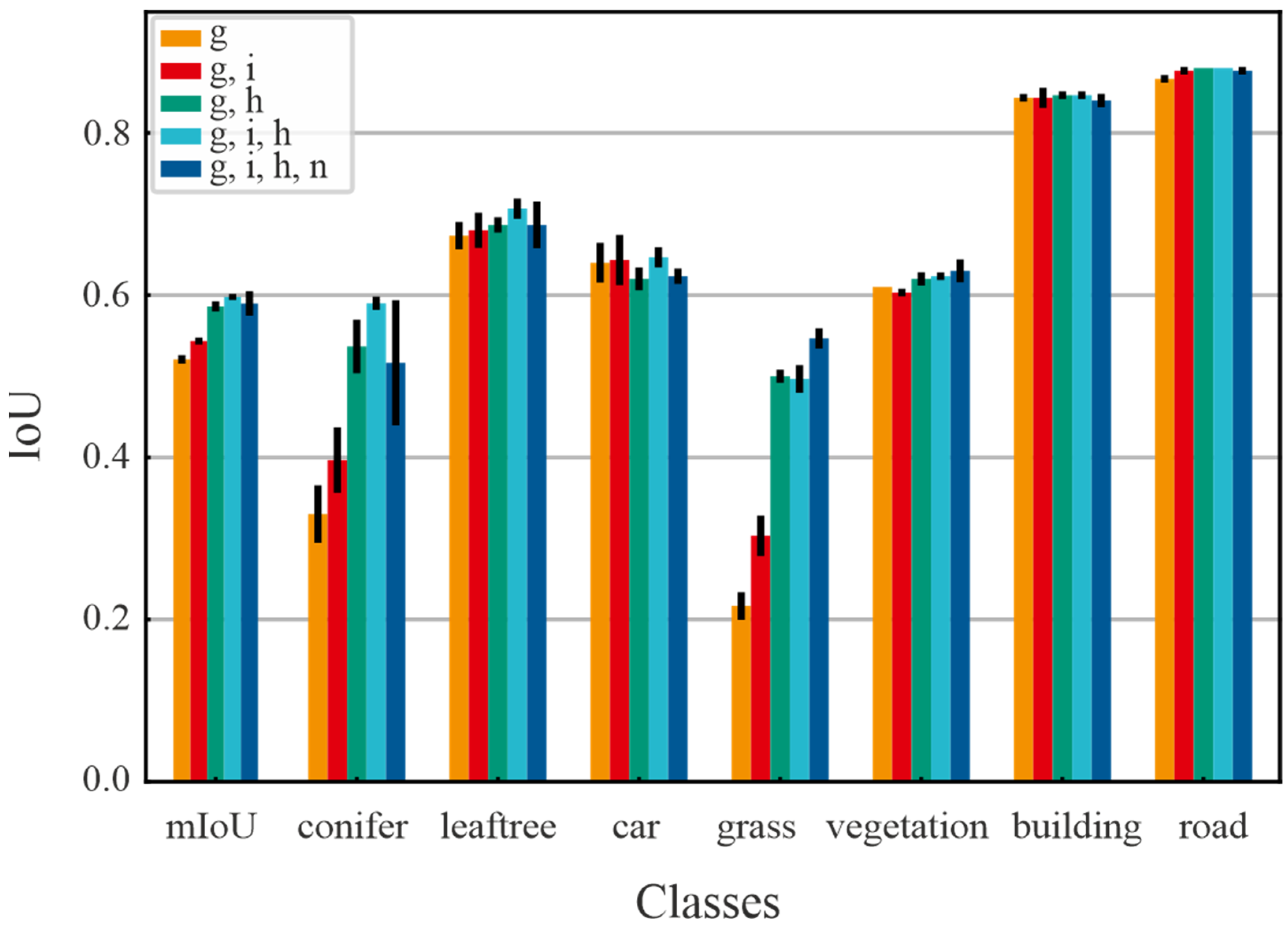
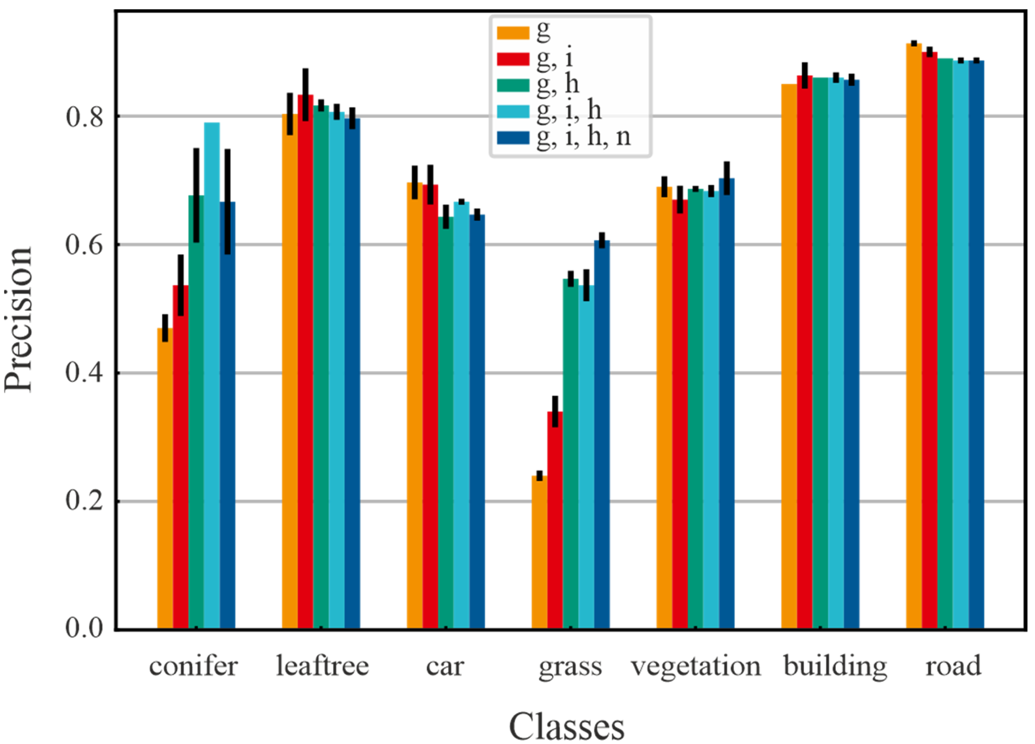
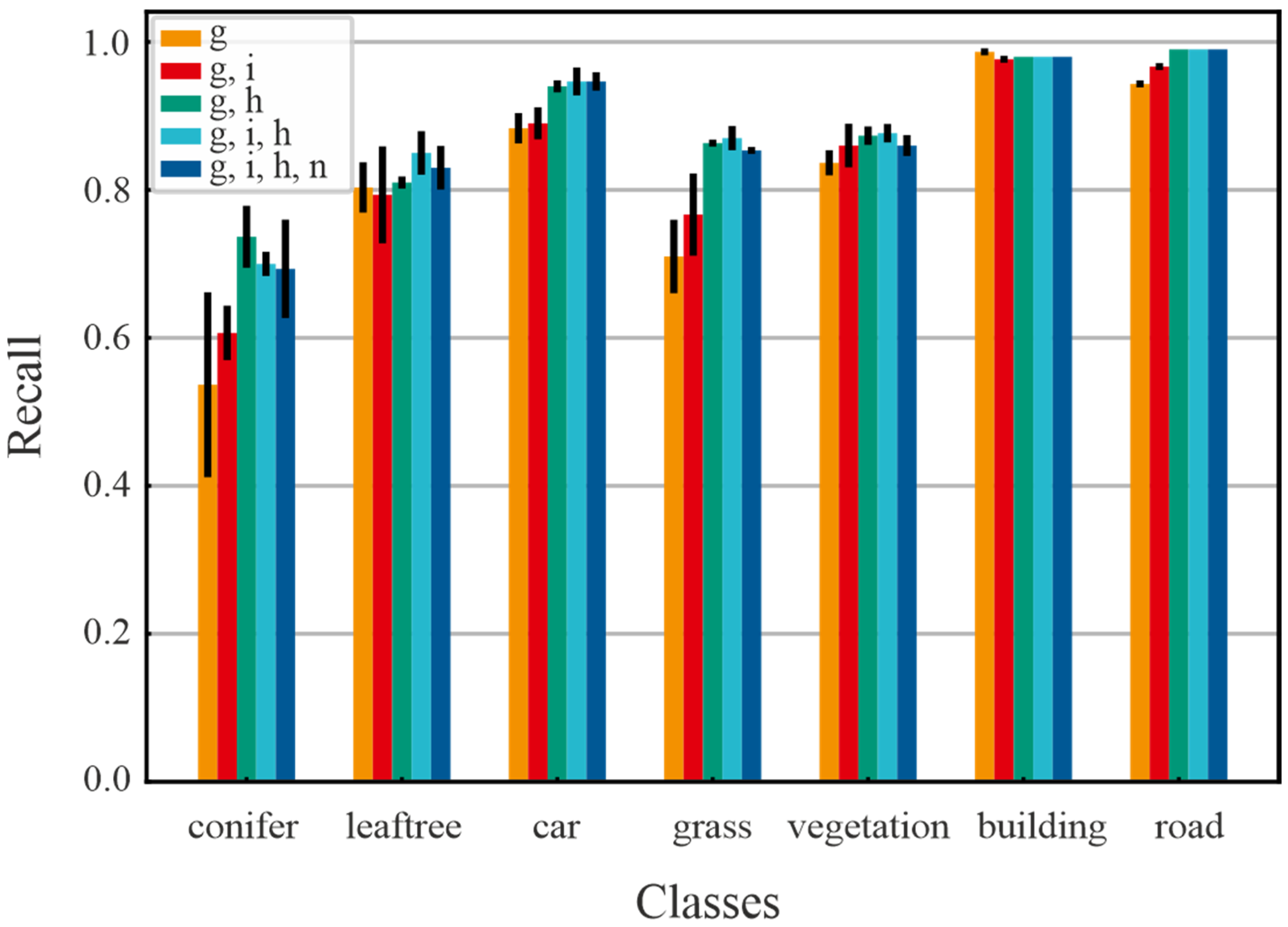
The mIoU and the IoU for every class are visualized in Figure 5. The values depict the average outcome of the three trainings for each setting while the error bars visualize the standard deviation. The corresponding values for the precision, recall and F1 score can be found in the Appendix A in Figure A1, Figure A2 and Figure A3. The results for mIoU for the three individual training courses vary only by around 1% which indicates a good convergence.

Using only geometric information the network achieved an mIoU of about 0.52.

When adding the intensity information, the mIoU increases by about 0.02 compared to only using geometric information. If using the DAV instead of the intensity it increases by about 0.07. Combining both results in an increase by about 0.08.

The resulting increases in IoU are strongly dependent on the classes. The IoU for the classes leaf tree, general vegetation, car, building and road show no significant dependency on any additional input channels besides the geometry. For the grass surfaces CNN performs poorly with the only input being the geometry. The additional use of the intensity leads to an increase in the IoU of grass by approximately 0.08. This benefit is overshadowed by the increase by approximately 0.28 from using the differential absorption value as additional input parameter compared to just using geometry. The conifer class shows a similar trend but here the uncertainty is higher due to the sparsity of the class in the dataset. Nevertheless, the results indicate that the additional information allows CNN to better differentiate them from leaf trees.

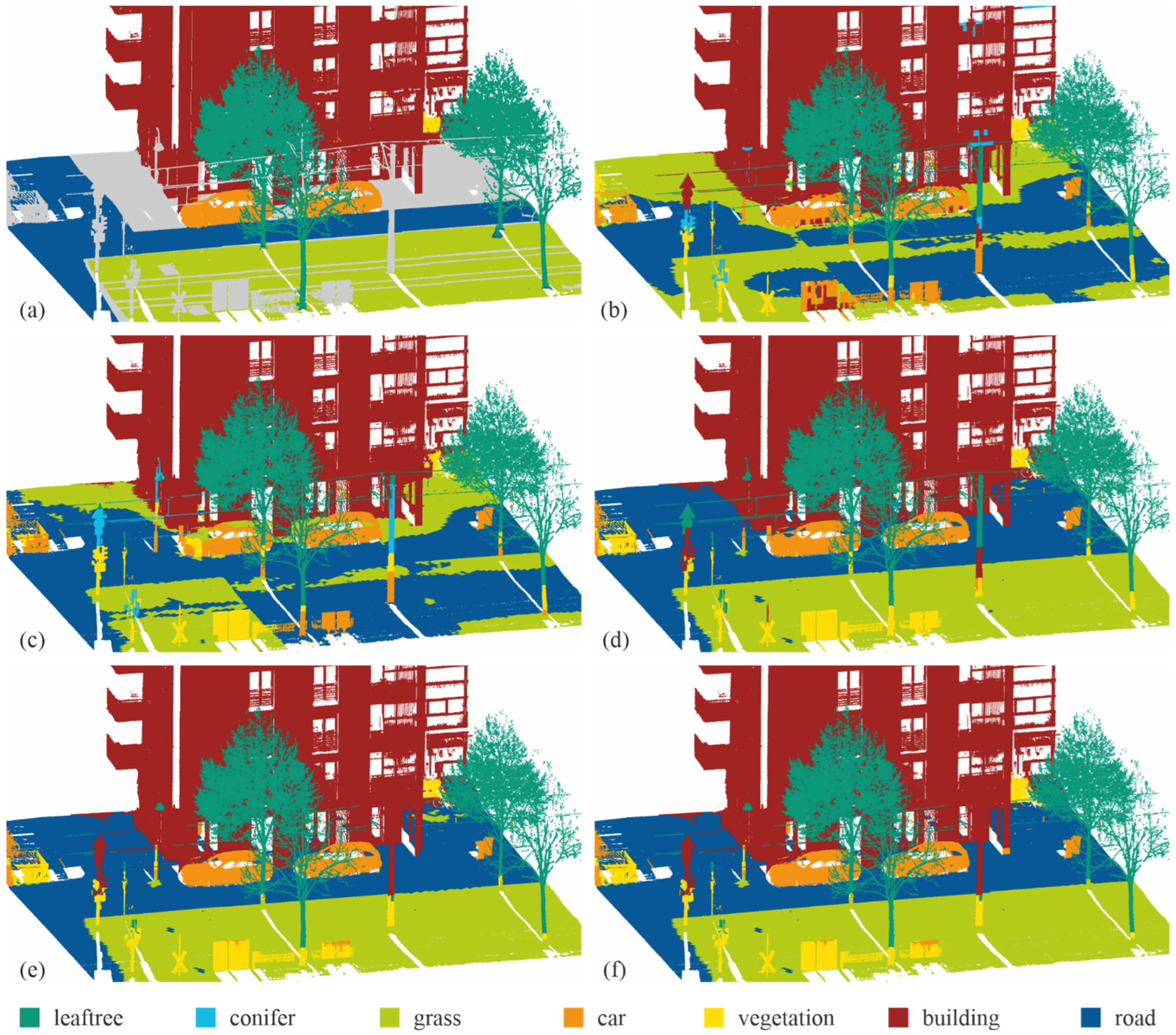
In Figure 6a–f the classification results are visualized via an exemplary point cloud, consisting of three adjacent 10 m sections from the validation dataset.

4. Discussion

The presented work evaluates the use of a novel multispectral LiDAR system, that operates at 1450 nm and 1320 nm wavelength to obtain additional information about the water content of surfaces for mobile mapping. The advantage over single wavelength LiDAR systems for automated semantic segmentation of point clouds by neural networks has been evaluated exemplary using a voxel-based discretization approach and a network architecture similar to 3D U-Net.

The results showed that for classes with high resemblance in geometry additional information about the surface remission can have a significant impact on the identification of objects in point clouds. Especially the additional use of multispectral data, using wavelengths selected according to the respective application, can greatly improve the classification results. In the presented study this was shown with the classification of grass surfaces in urban residential areas by using a differential absorption value, calculated from the remissions of the wavelengths 1320 nm and 1450 nm. The IoU could be increased from approximately 0.2 to 0.5 by adding the differential absorption value to the 3D information. This drastic increase can be explained by the fact that the geometric properties of grass surfaces are almost identical to those of road which has a higher occurrence in the dataset and is therefore prioritized by the CNN without any additional information. The over a factor of 3 stronger increase by adding the differential absorption value compared to adding the intensity can be explained by the strong effect of the water containing grass on the differential absorption value while the intensity generally shows fluctuations depending on surface topology and texture.

The classes leaf trees, general vegetation, car, building and road seem to show enough characteristic features in their spatial distribution of voxels that allow the CNN to solemnly differentiate between them based on this information. Here the use of additional information about the intensity or the differential absorption value leads to no significant increase in the IoU.

One also has to note that the measurements were done in November which meant that a lot of trees had already lost their leaves. This might have affected the classification results for leaf trees since the variation in differential absorption value for leaf trees varied from almost 0 for trees without leaves to 0.5 for trees which still had many leaves left.

Now, more data and more detailed experiments, especially also using non discretized approaches, are necessary to evaluate the effect in individual use case scenarios and to compare it to state-of-the-art mobile mapping using RGB-cameras and projection into the point cloud.

It would also be of interest whether the additional information would affect the results of RGB-based classification systems.