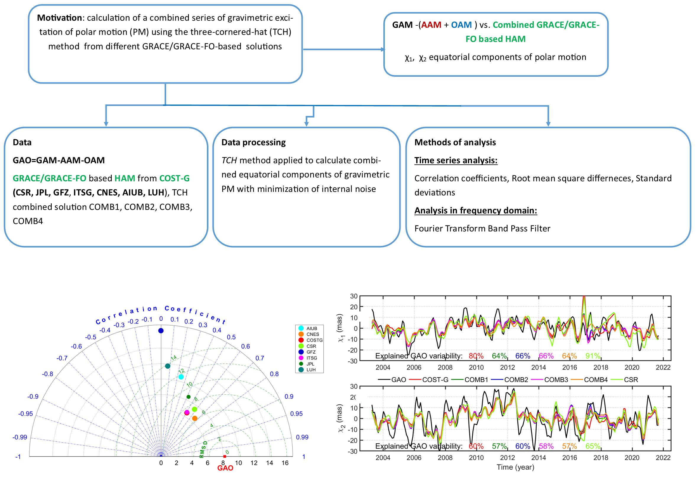
Exploiting the Combined GRACE/GRACE-FO Solutions to Determine Gravimetric Excitations of Polar Motion

Abstract

Observations from the Gravity Recovery and Climate Experiment (GRACE) and GRACE Follow-On (GRACE-FO) missions can be used to estimate gravimetric excitation of polar motion (PM), which reflects the contribution of mass changes in continental hydrosphere and cryosphere to PM variation. Many solutions for Earth’s gravity field variations have been developed by institutes around the world based on GRACE/GRACE-FO data; however, it remains inconclusive which of them is the most reliable for the determination of PM excitation. In this study, we present a combined series of GRACE/GRACE-FO-based gravimetric excitation of PM computed using the three-cornered-hat (TCH) method, wherein the internal noise level in a combined solution is reduced to a minimum. We compare the combined series with results obtained from the combined GRACE/GRACE-FO solution provided by COST-G (International Combination Service for Time-variable Gravity Fields) and from the single solution elaborated by the Center for Space Research (CSR). All the gravimetric excitation series are evaluated by comparison with the sum of hydrological and cryospheric signals in geodetically observed PM excitation (called GAO). The results show that by minimizing the internal noise level in the combined excitation series using the TCH method, we can receive higher consistency with GAO than in the case of COST-G and CSR solutions, especially for the non-seasonal oscillations. For this spectral band, we obtained correlations between GAO and the best-combined series as high as 0.65 and 0.72 for the χ₁ and χ₂ equatorial components of PM excitation, respectively. The corresponding values for seasonal oscillation were 0.91 for χ₁ and 0.89 for χ₂. The combined series developed in this study explain up to 68% and 60% of overall GAO variability for χ₁ and χ₂, respectively.

1. Introduction

The rotation of our planet is complex and no full analytical model for this phenomenon has been developed so far. Such complexity arises from the occurrence of a number of geophysical processes that constantly affect the speed of the Earth’s rotation and the orientation of its rotational axis. These disturbances mainly result from the global mass distribution of surficial fluid layers (atmosphere, ocean, and continental hydrosphere) and the interactions between them, the movements of the solid part of the Earth, and the gravitational influence of celestial bodies [1,2]. It is believed that since the beginning of the 21st century, the dynamics of the Earth’s rotation have also been affected by climate change and the ice mass loss in polar regions [3].

Polar motion (PM) is one of the Earth’s orientation parameters (EOP) and is defined as the motion of the Earth’s rotational axis with respect to the crust. PM is described with xp and yp coordinates given in a Cartesian plane coordinate system with the xp axis pointed along the Greenwich meridian and the yp axis pointed to the west. Similar to other EOPs, PM is affected by all above-mentioned phenomena with varying intensity and temporal variability. The variation of PM consists of several oscillations of different amplitudes and frequencies, the interpretation and finding of the sources of which is an important challenge that takes place on the boundary between geodesy and geophysics.

With the growing accuracy of (xp, yp) measurements, scientific interest in interpreting the variation in PM resulting from changes in the distribution of mass of the Earth’s fluid layers has increased [1,3,4,5,6,7,8,9,10,11,12]. Such analyses have recently increased in importance and quality because, since 2002, the Gravity Recovery and Climate Experiment (GRACE) and GRACE Follow-On (GRACE-FO) satellite missions have been able to monitor temporal changes in the Earth’s gravitational field on a global scale and with unprecedented accuracy [13,14]. The missions’ observations are processed by many institutes around the world in order to elaborate and distribute time-variable gravity field models mainly in the form of sets of spherical harmonic (SH) coefficients of geopotential. Such models can be exploited to investigate gravimetric excitation of PM thanks to a linear relationship between equatorial components (χ₁, χ₂) of the excitation function and the degree-2 order-1 coefficients of geopotential (ΔC₂₁, ΔS₂₁) [15,16]. Since the non-tidal atmospheric and oceanic effects are routinely removed from the GRACE/GRACE-FO solutions, the resulting excitations mainly reflect the impact of the continental hydrosphere and cryosphere on PM excitation and are also interchangeably called gravimetric excitation [17,18,19,20], hydrological excitation or hydrological angular momentum (HAM) [11,21], hydrological plus cryospheric excitation, or hydrological plus cryospheric angular momentum (HAM/CAM) [22,23,24].

Although many studies have used various GRACE/GRACE-FO solutions to determine gravimetric excitation of PM in recent years [5,7,10,11,16,25,26,27,28,29], the most reliable solution for use in studies of hydrological and cryospheric signals in PM variation has not yet been conclusively identified. This is largely because of the non-negligible differences between PM excitation estimates derived from data provided by various data centres. There is an increasing number of new solutions developed by an increasing number of institutes dealing with GRACE/GRACE-FO data processing, which creates a need to validate the newly delivered data. In our previous study [23], we assessed a PM excitation series based on different types of GRACE/GRACE-FO data from one data centre and we showed that depending on the GRACE/GRACE-FO data used and equatorial component considered, root mean square deviation for GRACE-based HAM/CAM values were between 6.3 and 10.9 mas for overall time series, between 1.9 and 4.7 for seasonal variation, and between 5.8 and 9.9 mas for non-seasonal variation. The choice of the most appropriate GRACE/GRACE-FO solution for the purpose of determination of PM excitation is a complex issue and depends on several factors such as the considered time period, analysed oscillation, and assumed criterion of evaluation [20].

In view of the existence of many available GRACE/GRACE-FO solutions, their combination is a very common approach in various research tasks. Authors in work [30] stated that compared with individual solutions, the combined GRACE series are characterized by lower noise (as measured with the root mean square of equivalent water height anomalies over the oceans) because of the removal of systematic errors typical to some processing centres, while the signal content of the individual contributions is preserved in the combination. Similar conclusions were drawn by [31], who combined GRACE monthly gravity field models processed with different computation approaches on the normal equation level. Authors of the work [30] showed that the combination of data provided by only three official GRACE Science Data System members (the Center for Space Research (CSR), Jet Propulsion Laboratory (JPL), and GeoForschungsZentrum (GFZ)), are noisier than combination based on a larger number of solutions. Therefore, it is acceptable to use also other datasets, such as those processed by the Institute of Geodesy at the Graz University of Technology (ITSG), the Centre National d’Études Spatiales (CNES), the Astronomical Institute of the University of Bern (AIUB), or Leibniz Universität Hannover (LUH), to develop a combined series.

Combining various monthly global gravity field models and making them available to the users is a task currently performed by the International Combination Service for Time-variable Gravity Fields (COST-G), which is a data centre of the International Gravity Field Service [32]. The members of COST-G routinely perform combinations of GRACE and GRACE-FO data from various analysis centres on both solution and normal equation levels and carry out their internal and external validation. COST-G also provides combined gravity solutions from Swarm data that act as an alternative to GRACE/GRACE-FO, especially during the periods of missing data that occur between and within GRACE and GRACE-FO [33]. Other temporal gravity field data products combine observations from different techniques or different satellites such as GRACE and satellite laser ranging (SLR) data [34], GRACE, SLR, and Swarm data [35], or SLR and high-low satellite-to-satellite tracking data [36].

Many previous studies have used either mean or combined GRACE/GRACE-FO solutions for different scientific applications such as analysis of geoid changes [37], total water storage variations [38], or groundwater storage changes [39]. In the current study, we focused on the use of combined GRACE/GRACE-FO data to determine gravimetric excitation of PM. Although the mean of several GRACE/GRACE-FO solutions has been used previously in the study of hydrological excitation of PM [11,18], this is the first research to use more advanced combinations of the gravimetric series. The main objective of this study is to develop a combination solely dedicated to estimating the PM excitation. To elaborate such a combination, we exploit the three-cornered hat (TCH) method [40] which allows us to determine the noise level in a single GRACE/GRACE-FO-based excitation series. Based on the estimated noise in the series, we determine the weights for individual solutions in a combined series. This approach allows us to minimize the noise level in a combined series of multiple solutions from different computing centres. The TCH method has been used previously in PM studies for the determination of the quality of atmospheric angular momentum (AAM) [41] and oceanic angular momentum (OAM) [42] estimates. The method allows the determination of errors in the series only on the basis of the determined values of their noise and without the need to use external reference data. Although it has been widely used in different research fields such as estimating the instabilities of clocks [43], studying errors of sea surface temperature observations [44], determining error variances of several atmospheric datasets [45], or estimating uncertainties in measurements of precipitation [46], the TCH method has not yet been used to estimate the combined gravimetric excitations of PM.

The combined excitation series developed in this study are subjected to a detailed analysis, which includes overall variability of time series, amplitude spectra, amplitudes and phases of annual oscillation, and non-seasonal variability. We also perform an external validation of the series by comparing them with hydrological plus cryospheric signals in observed (geodetic) excitation called geodetic residuals (GAO). The GAO series provides important reference data for the validation of HAM determined not only from GRACE/GRACE-FO data but also from hydrological models [27,28] or climate simulations [47]. Similar comparisons of GAO with HAM computed from various data sources were considered in previous studies [5,10,19,20,21,27,28,29,48,49]. These studies showed a high diversity in the HAM series obtained from not only different land hydrosphere and climate models but also from GRACE/GRACE-FO data provided by the various processing centres. In addition, achieving full compatibility between GAO and HAM solutions is contingent on the uncertainties in atmospheric and oceanic models that affected the GAO time series [50,51].

The combined series developed with the use of the TCH method are also compared with those received for COST-G data. The main objective of the current work is to examine whether the combination made by the TCH method noticeably increases the correspondence between the hydrological plus cryospheric signal in gravimetric and geodetic excitation of PM compared with the compliance obtained for single GRACE/GRACE-FO solutions or the series provided by COST-G.

Apart from GRACE data, C₂₁ and S₂₁ coefficients obtained from SLR have also been used to determine PM excitation (e.g., [23,52]). However, in the current study, we do not consider SLR as it was discussed in our previous work [23]. In that paper, we showed that SLR provides consistency between HAM/CAM and GAO not as high GRACE/GRACE-FO data, especially in terms of seasonal oscillations, because of underestimating amplitudes of GAO. However, SLR can be useful for estimating HAM/CAM in non-seasonal spectral bands.

The structure of the paper is as follows. Section 2 describes the data and methodology used, specifically, Section 2.1 includes information about geodetic residuals (GAO) used as a reference in the validation of combined gravimetric PM excitation series, Section 2.2 presents a description of GRACE/GRACE-FO data and method of computing gravimetric excitation of PM, Section 2.3 explains the principle of the TCH method, and Section 2.4 describes the method of developing the combined series of gravimetric excitation of PM. Section 3 presents results for the overall (Section 3.1), seasonal (Section 3.2), and non-seasonal (Section 3.3) variations. Finally, Section 4 provides a discussion of the results and presents conclusions.

2. Data and Methodology

2.1. Reference Geodetic Residual Time Series

We calculated χ₁ and χ₂ equatorial components of the hydrological plus cryospheric signal in observed PM excitation by subtracting atmospheric excitation AAM (sum of the mass term related to atmospheric pressure and motion term related to winds) and ocean excitation OAM (sum of the mass term related to ocean bottom pressure and motion term related to ocean currents) from geodetic excitation GAM:

$$GAO=GAM-AAM-OAM$$

(1)

where GAM is determined from precise geodetic measurements of pole coordinates and AAM and OAM are based on geophysical models of the atmosphere and oceans, respectively. The resulting series is also denoted as geodetic residuals or GAO.

In this study, daily series of GAM was obtained from the International Rotation and Reference System Service (IERS), Earth Orientation Center (https://hpiers.obspm.fr/eop-pc/index.php, accessed on 1 July 2022), and based on xp and yp pole coordinates from the EOP 14 C04 solution [53]. The EOP 14 C04 series is based on a combination of different space geodetic techniques, while maintaining consistency with the International Terrestrial Reference Frame (ITRF2014 [54]) and implementing the latest IAU 2006/200A precession-nutation model.

χ₁ and χ₂ components of GAM can be computed using the Liouville algorithm (e.g., [55], https://hpiers.obspm.fr/eop-pc/index.php, accessed on 1 July 2022):

$$\dot{p}-i{\sigma }_{c}p=-i{\sigma }_c\chi ,$$

with pole coordinates $p=xp+iyp$ and complex Chandler frequency ${\mathsf{\sigma }}_{\mathrm{c}}=2\mathsf{\pi }\left(1+\mathrm{i}/2\mathrm{Q}\right){\mathrm{T}}_{\mathrm{c}}$, with a Chandler period $T_c=433$ days and a damping Q = 100. In previous studies, the GAM series have been computed with different Chandler periods T and Chandler quality factor Q equal to 433 days and Q = 179 [56] or with the Chandler period equal to 430.9 and Q = 127 [57]. The equatorial excitation function is based upon the knowledge of the Chandler term period T and its quality factor Q. As these parameters are affected by large uncertainties, it is recommended to use these factors in the following intervals: 426 < T < 439 days; 50 < Q < 200 [58].

There exists another time series of terrestrial pole coordinates, xp and yp, that can be transformed into time series of GAM (e.g., combined EOP solutions provided by JPL, so-called JPL-Comb2018 solution, and EOP series obtained from single space geodetic techniques). These geodetic series reveal very similar variations for periods longer than a week [59] and differences between them should not affect our results as we consider monthly data sampling.

Both AAM and OAM series used in this study were processed and provided by the Earth System Modeling group at GFZ (ESMGFZ). The ESMGFZ routinely provides the effective angular momentum functions (EAMF) of the atmosphere, ocean, and hydrosphere describing the nontidal geophysical excitations of the Earth’s orientation changes due to mass redistribution of these fluid layers [60]. The AAM series provided by GFZ are based on the ECMWF (European Center for Medium-Range Weather Forecasts) model [6], whereas the OAM series are processed using the MPIOM (Max Planck Institute Ocean Model) model.

The temporal resolution of the ECMWF model used by ESMGFZ to compute AAM is 3 h. Tidal variations for the 12 most relevant frequencies are fitted and removed by ESMGFZ from the data to retain the nontidal signal only [61]. ESMGFZ AAM functions are calculated from numerical weather model data provided by the ECMWF. The series were calculated from operational atmospheric forcing data, given at 25 pressure levels with the model top at 1 hPa. The inverted barometer (IB) correction is applied to surface pressures from all oceanic locations of the underlying 0.5° grid [55].

The OAM MPIOM oceanic model, discretized on a ten-tripolar grid and 40 vertical layers [62], is forced with operational ECMWF analysis fields, including instantaneous surface stresses calculated offline from horizontal winds at 10 m and boundary layer stability theory [63]. The MPIOM model solves the primitive equations with the hydrostatic and Boussinesq approximations [63]. The OAM MPIOM series are calculated with the same atmospheric data from the ECMWF model that was used for AAM. The IB correction is also applied to ocean bottom pressures, and the oceanic response to atmospheric tides is estimated and removed from both mass and motion terms. The OAM data are available with the same temporal sampling and at the same frequency as the AAM from ESMGFZ. The AAM and OAM series were received from the ESMGFZ website (http://rz-vm115.gfz-potsdam.de:8080/repository, accessed on 1 April 2022).

The ECMWF and MPIOM models have been also applied in GRACE/GRACE-FO de-aliasing data (atmosphere and ocean de-aliasing Level-1B release-6 or AOD1B RL06) used to eliminate atmospheric and oceanic non-tidal contributions from gravity fields. Therefore, in terms of AAM and OAM errors, the consistency between GAO and gravimetric excitation determined in this study should be as high as possible.

Previous studies [21,22,26] considered different AAM and OAM models in GAO determination. Hence, information about the internal quality of AAM and OAM models is well known. Generally, the total mass and motion of both AAM and OAM excitations are calculated with root-to-mean square differences about a couple of mas, wherein these differences are higher from OAM models (e.g., [60]). In particular, [42] used the TCH method to analyze four OAM models and showed that in the case of changes with periods of a month and longer, the values of the standard deviation of noise in OAM were as high as 1–3 × 10⁻⁸, which gave about 2–6 mas. In the case of unfiltered series (without removing short-term oscillations), these values were 4–22 mas. In turn, [41] used TCH method to analyze five AAM models and showed that the standard deviation of noise in the AAM series, depending on the model and time interval, ranged from 7 to 20 mas, which was a similar level to that obtained by [42] for OAM. However, taking into account the fact that the influence of AAM on the excitation of pole motion is greater than the influence of OAM (larger amplitudes, larger standard deviation of the series), the signal-to-noise ratio for OAM is less favorable, and therefore it can be concluded that OAM models are characterized by greater uncertainties than AAM models.

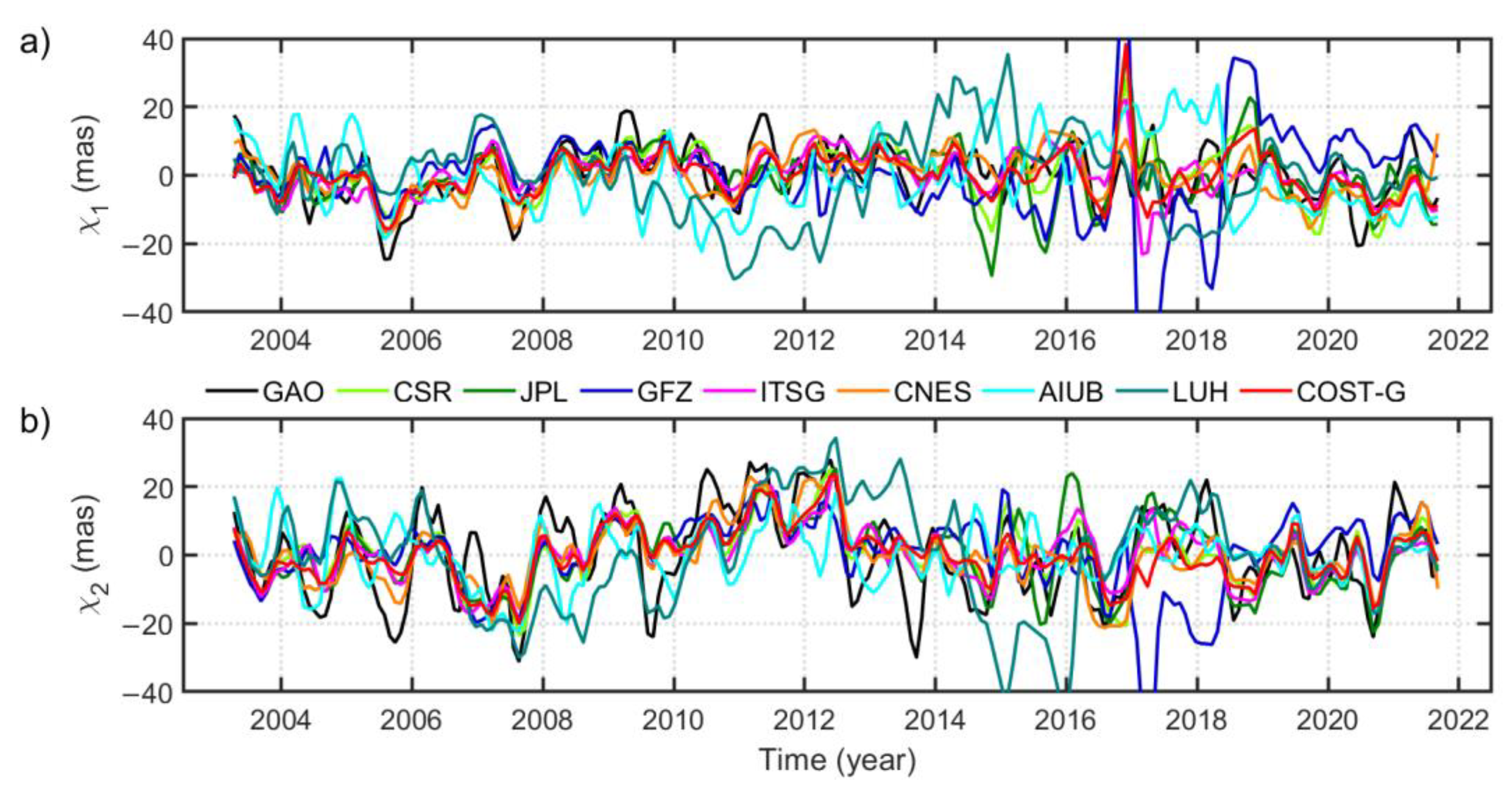
2.2. Gravimetric Excitation Series from GRACE and GRACE-FO Solutions

Equatorial components (χ₁, χ₂) of gravimetric PM excitation can be computed with the use of the following equations that describe the linear relationship between (χ₁, χ₂) and changes in degree-2 order-1 coefficients of geopotential (ΔC₂₁, ΔS₂₁) delivered by GRACE and GRACE-FO [55]:

$${\chi }_1=-\sqrt{\frac{5}{3}\cdot }\frac{1.608\cdot R^2\cdot M}{C-A{}^{\prime }}\mathsf{\Delta }{C}_{21},$$

(2)

$${\chi }_2=-\sqrt{\frac{5}{3}\cdot }\frac{1.608\cdot R^2\cdot M}{C-A{}^{\prime }}\mathsf{\Delta }{S}_{21}$$

(3)

where R is the Earth’s mean radius; M is the Earth’s mass; A, B, and C are the principal moments of inertia for Earth (A = 8.0101 × 10³⁷ kg·m², B = 8.0103 × 10³⁷ kg·m², and C = 8.0365 × 10³⁷ kg·m², from [55]), A’ = (A + B)/2 is an average of the equatorial principal moments of inertia [64], and $\mathsf{\Delta }$C₂₁ and $\mathsf{\Delta }$S₂₁ are the normalized SH coefficients of geopotential. Factor 1.608 includes the modification of the Love load number due to the mantle and elasticity [16].

First, we applied Equations (2) and (3) to compute (χ₁, χ₂) from the newest available realizations of the following single GRACE/GRACE-FO solutions:

• CSR RL06 (for both GRACE and GRACE-FO period)—provided by the Center for Space Research, Austin, USA, abbreviated here as CSR;
• JPL RL06 (for both GRACE and GRACE-FO period)—provided by the Jet Propulsion Laboratory, Pasadena, USA, abbreviated here as JPL;
• GFZ RL06 (for both GRACE and GRACE-FO period)—provided by GeoForschungsZentrum, Potsdam, Germany, abbreviated here as GFZ;
• ITSG-Grace2018 (for GRACE period) and ITSG-Grace_op (for the GRACE-FO period)—provided by the Institute of Geodesy at Graz University of Technology, Graz, Austria, abbreviated here as ITSG;
• CNES/GRGS RL05 (for both GRACE and GRACE-FO period)—provided by the Centre National d’Etudes Spatiales/Groupe de Recherche de Géodésie Spatiale, Toulouse, France, abbreviated here as CNES;
• AIUB RL02 (for GRACE period) and AIUB-GRACE-FO_op (for the GRACE-FO period)—provided by the Astronomical Institute University Bern, Bern, Switzerland, abbreviated here as AIUB;
• LUH-Grace2018 (for GRACE period) and LUH-GRACE-FO-2020 (for the GRACE-FO period)—provided by Leibniz Universität Hannover, Hannover, Germany, abbreviated here as LUH.

Each of the above datasets is used by scientists involved in developing a combined GRACE/GRACE-FO solution under the COST-G initiative. Therefore, the combined series of gravimetric excitations developed in this study are also compared later in the article with those calculated from COST-G data. All single and combined GRACE/GRACE-FO solutions have been accessed from the International Centre for Global Earth Models (ICGEM) website (http://icgem.gfz-potsdam.de/home, accessed on 1 April 2022).

The nearly one-year gap (June 2017 to June 2018) between the excitation series computed from GRACE data and the corresponding series based on data from GRACE-FO was filled by performance forecasting using the seasonal ARIMA (autoregressive integrated moving average) method, with the arima function available in MATLAB [65].

All detrended gravimetric excitation series determined from seven GRACE/GRACE-FO single solutions (CSR, JPL, GFZ, ITSG, CNES, AIUB, and LUH) and one combined (COST-G) solution after gap filling are depicted in Figure 1. All of these are later used to process the combined series of gravimetric excitation, as described in the next subsection. The series of GAO is also shown for comparison. The trends in PM excitation, which result mainly from post-glacial rebound and ice mass changes [55], are not studied here. Figure 1 shows that in the initial period of GRACE activity (between 2003 and 2010), despite some observable differences in amplitude, all series generally follow a consistent course. The inconsistencies between the individual series increase and the discrepancies are largest for the period 2014–2018. This is related to the progressive degradation of the instruments on board satellites, particularly the declining battery capacity and the turning off of one of the accelerometers in 2017. The consistency between all series is highest in the period of GRACE-FO measurements (after 2018), which confirms the progress made in terms of both the quality of the measurements and the methods of data processing [13]. For the period of GRACE activity, the series based on the LUH and AIUB solutions are inconsistent with the other solutions, which is especially apparent for χ₁ in the periods between 2009 and 2012, and between 2014 and 2015, and for χ₂ in the periods between 2008 and 2010, and between 2012 and 2016. This may be because, for the period of GRACE, LUH, and AIUB, temporal gravity models were developed based on older background models and parameterization methods than in the newest solutions from other institutes [66,67]. Consequently, AIUB and LUH are more comparable with previous releases (RL05) of solutions from official GRACE/GRACE-FO data centres at CSR, JPL, and GFZ, which are not considered here as we focus on the latest available datasets. For the period of GRACE-FO activity, the teams from AIUB and LUH updated the data-processing methods and background models used, which resulted in an increased consistency with other solutions. Figure 1 shows that the series based on the GFZ solution differs from the others in the period between 2016 and 2018, which is probably related to the inaccurate modelling of surface forces and inappropriate parametrization [68]. The series based on the COST-G solution is characterized by lower amplitudes than the others, indicating that the combination of many individual solutions may effectively minimize the noise in the series.

Results of the initial evaluation of the gravimetric excitation series obtained from the above-mentioned solutions are shown in Figure 2 which presents Taylor diagrams with the values of standard deviation (STD), zero-lag correlation coefficients (Corr), and root mean square differences (RMSD) [69]. Here, Taylor diagrams provide a graphic summary of how closely a pattern of gravimetric excitation series matches a reference, namely GAO. The critical values of Corr were taken from the statistical tables for the standard Student’s t-test for the computed number of independent points and the assumed confidence level (95%) ([11]). The number of independent points was calculated by dividing the length of the series (in our case 225) by the decorrelation time (time after which the autocorrelation function drops to 1/e, which was different for different oscillations considered in this study). The standard error of the difference between the two Corr was obtained as a $\sigma =\sqrt{2/\left(N-3\right),}$ where N is the number of independent points.

Figure 2 shows that the dispersion of the results obtained from individual solutions is quite high. The Corr values range from 0.00 (GFZ) to 0.66 (CNES) for χ₁ and from 0.19 (GFZ) to 0.76 (CNES) for χ₂, RMSD values are between 6.24 (CNES) and 18.18 mas (GFZ) for χ₁ and between 8.47 (CNES) and 15.79 mas (LUH) for χ₂, while STD values are as high as 6.55 (COST-G) to 16.26 (GFZ) mas for χ₁ and 7.85 (COST-G) to 15.68 (LUH) mas for χ₂. The analysis of STD values shows that depending on the solution exploited, gravimetric excitation series either underestimate or overestimate the variability observed for GAO. The CNES-based series have the highest consistency with GAO. However, it should be remembered that the CNES solution has been processed as a combination of GRACE/GRACE-FO data with SLR observations, so it cannot be considered a purely single GRACE/GRACE-FO solution such as CSR, JPL, GFZ, ITSG, AIUB, and LUH. Of all single solutions, CSR provides the highest consistency between gravimetric excitation and GAO. Notably, the COST-G-based series does not provide as high an agreement with GAO as CSR and CNES, so we suggest that COST-G is not an optimal combination for a PM excitation study.

2.3. The Generalized TCH Method

In the absence of a reference dataset with known errors, the TCH method can be used to estimate the relative uncertainties of the gravimetric PM excitation time series. To achieve this, at least three different sources of time series representing the same process are needed. This method was introduced by [70] and was originally used to estimate the stability of oscillators and clocks. It has since become increasingly important in the evaluation of uncertainty in EOP measurements, and geophysical excitation functions of PM and length of the day [15,21,41,71,72].

A powerful technique for simultaneously estimating random error statistics of three datasets, the TCH method, is the simplest case (N = 3) of the more general N-cornered hat method, which uses N datasets. This method was developed by [73] to estimate the errors of three different instruments. While widely used in the physics community, the 3CH method has not been used to estimate the errors of geophysical excitation functions of PM until recently (e.g., [41,42]). In general, the TCH method allows an estimation of the noise level in the time series only by comparing them against each other [40]. This is done with some assumptions on the correlations between the examined noises in series. Different formulations of the TCH method can be used, depending on the assumptions made on the correlations between the noises. In this study, we applied a generalized TCH method that does not assume zero correlation between the series tested [41,42]. Here, the computation of the noise variance in gravimetric excitation series with the use of the TCH method is based on the differences between individual series and one selected series treated as a reference (here CSR RL06), and then minimizing the global correlation among the noises in the individual time series. We use the CSR RL06 solution as a reference since we previously showed that this solution provides higher consistency between the GAO and gravimetric excitation series than other solutions (see [20] and Figure 2 in this study). Nevertheless, the choice of reference series should not have an impact on the resulting combined series of gravimetric excitation [41].

From the mathematical point of view, if we consider the time series stored as ${\left\{X_i\right\}}_{i=1,2,\dots ,N}$, where i corresponds to each solution of gravimetric excitations time series (N), the TCH method split them into two terms:

$$X^i=S+{\epsilon }^i, i=1,\dots ,N,$$

(4)

where S is defined as the part of the series that is common to all of them and represents the true signal, and ${\epsilon }_i$ is a noise remaining in each gravimetric excitations time series. With this definition, the information about the noise level of each gravimetric excitations time series may be obtained by determining the differences between these series.

The principle of the generalized TCH method is described below.

We take the difference between each series and one of them (CSR RL06) arbitrarily chosen as a reference:

$$Y^{iN}=X^i-X^N={\epsilon }^i-{\epsilon }^N, i=1, \dots , N-1,$$

(5)

where $X^N$ is a reference time series. The samples of the N − 1 solution centres’ differences, each length equal to M, are concatenated in an $M\times \left(N-1\right)$ matrix as:

$$Y=\left[Y^{1N} Y^{2N}\dots Y^{\left(N-1\right)N} \right].$$

(6)

The covariance matrix S of the residual time series of their differences is computed as:

$$S=cov\left(Y\right).$$

(7)

We introduce the $(N\times N$) Allan covariance matrix of the individual noises R, whose elements are the unknowns of the problem and will be determined by relation to S as:

$$S=H^T·R·H, \mathrm{with} H=\left[\begin{array}{c}I\\ -u^T\end{array}\right].$$

(8)

Equation (9) can be rewritten as:

$$S=\left[I-u\right]\left[\begin{array}{cc}\widehat{R} & r\\ r^T& r_{NN}\end{array}\right]\left[I-u^T \right],$$

(9)

where $I$ is the identity matrix and $u$ is the ${\left[1 1 1\dots 1\right]}^T$ vector, $\widehat{R}$ is the $\left(N-1\right)\times \left(N-1\right)$ submatrix, and $r$ is the $\left(N-1\right)$ vector grouping the covariance estimates that involve the $N{}^{\prime }$th time series, and $r_{NN}$ is the variance of the $N{}^{\prime }$th reference series.

Next, we isolated the $N$ free parameters of Equation (9) by the minimization of the global correlation among the noises of the individual time series using objective function, according to the Kuhn–Tücker theorem:

$$F\left(r,r_{NN}\right)={\sum }_{i:j} \frac{r_{ij}^2}{{\left(det\left(S\right)\right)}^{\frac{2}{N-1}}},$$

(10)

with a constraint function [72]:

$$G\left(r, r_{NN}\right)\equiv -\frac{r_{NN}-{\left[r-r_{NN}u\right]}^T·S^{-1}·\left[r-r_{NN}u\right]}{{\left(det\left(S\right)\right)}^{\frac{1}{N-1}}}<0.$$

(11)

The initial conditions were selected to provide that the initial values achieve the constraints [74]:

$$r_{iN}^{\left(0\right)}=0, i<N and r_{NN}^{\left(0\right)}={\left(2·u^T·S^{-1}·u\right)}^{-1}.$$

(12)

After determining the free parameters, the remaining unknown elements of $\hat{R}$ matrix is determined as follows:

$$\widehat{R}=S-r_{NN}\left[u{u}^T\right]+u{r}^T+r{u}^T.$$

(13)

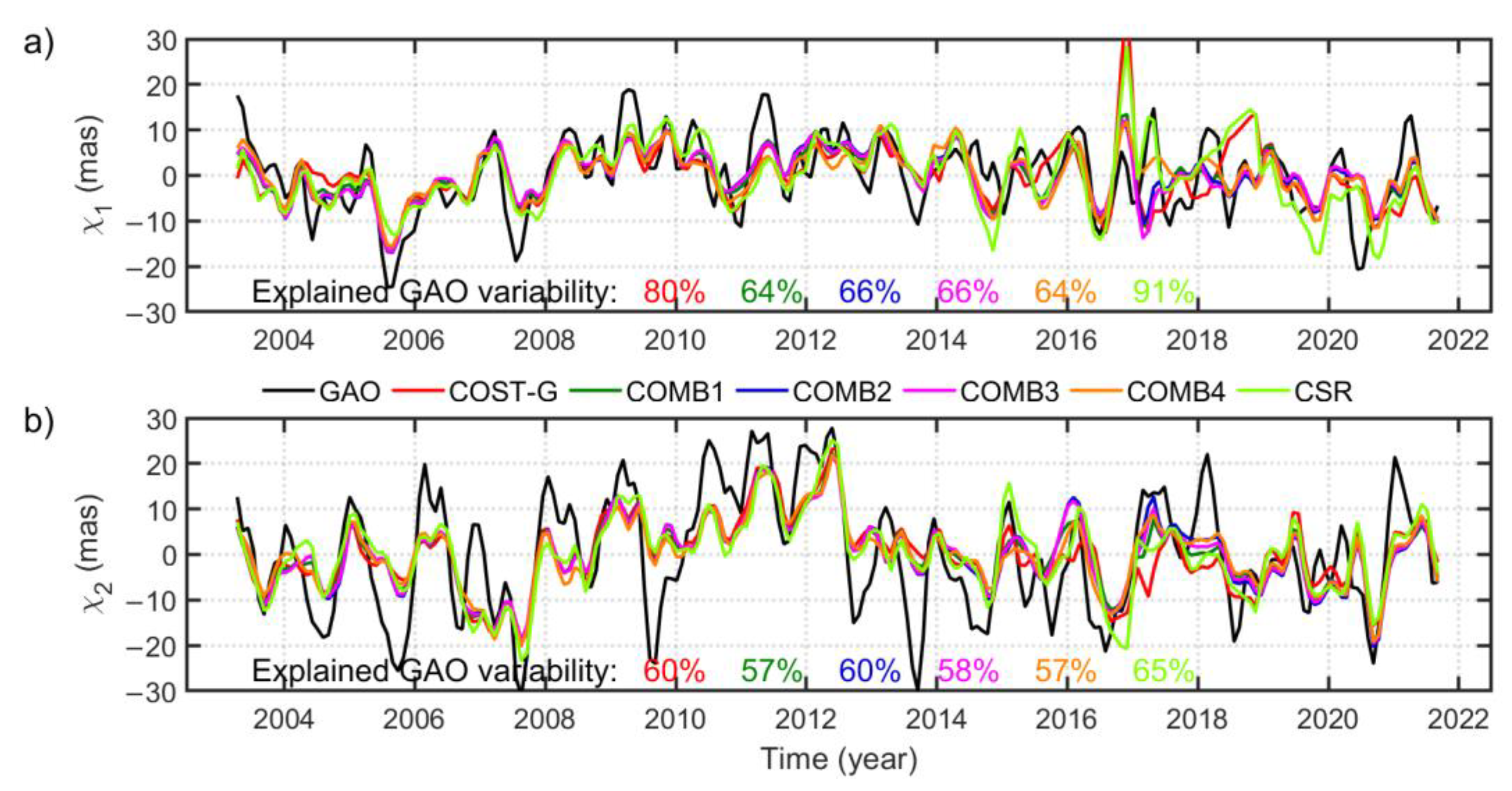
2.4. A Combined GRACE/GRACE-FO-Based Excitation Time Series

We assume that the noise level in each GRACE/GRACE-FO-based excitation series may differ noticeably, and the best representation of the hydrological signal in PM excitation is a combination of several series. We made a combination of the excitation series computed from GRACE/GRACE-FO data, taking their quality into account, such that the combined time series has a noise level as low as possible.

After finding the noise level in each gravimetric excitation series, we computed the combined (COMB) series of gravimetric excitation with a combination of the N series:

$$\left[\begin{array}{c}{\chi }_1^{COMB} \\ {\chi }_2^{COMB}\end{array} \right]={\sum }_{i=1}^N w_i\left(t\right)\left[\begin{array}{c}{\chi }_1^i\left(t\right) \\ {\chi }_2^i\left(t\right)\end{array} \right],$$

(14)

where $w_i\left(t\right)$ is the weight associated with the ${\chi }_1^i$ and ${\chi }_2^i$ equatorial components of PM excitation.

The condition of minimal noise variance for the combined time series gives the following normalized weights as a solution:

$$w_i=\frac{\frac{1}{Var\left({\epsilon }_i\right)}}{{\sum }_{j=1}^N \frac{1}{Var\left({\epsilon }_j\right)}}.$$

(15)

The combined series developed in this study with the TCH method are weighted mean, where the weights calculated for each series are inversely proportional to the noise variance of the series.

Based on a visual inspection of the series and their initial preselection (Figure 1 and Figure 2), we decided to develop four combined gravimetric excitation series, here called COMB solutions:

• COMB1: a combination of data from CNES, COST-G, ITSG, JPL, and CSR;
• COMB2: a combination of data from CNES, ITSG, JPL, and CSR;
• COMB3: a combination of data from CNES, ITSG, JPL, CSR, and GFZ;
• COMB4: a combination of data from CNES, JPL, CSR, LUH, AIUB.

As gravimetric excitation series from GFZ, AIUB, and LUH turned out to differ visibly from the other series and from GAO (Figure 1 and Figure 2), they were included only in chosen combined solutions (GFZ is included only in COMB3, and LUH and AIUB are included only in COMB4). We also consider one combined series (COMB1) in which data from COST-G are exploited. Since CNES, JPL, and CSR solutions were revealed to produce the highest consistency with GAO, they were included in all four combined series. The COMB2 series includes all single solutions except GFZ, LUH, and AIUB, which turned out to have the lowest consistency with GAO.

Table 1. Weights for GRACE/GRACE-FO solutions in each COMB solution were determined with the TCH method. The highest weights are bolded.

	COMB1 Weights		COMB2 Weights		COMB3 Weights		COMB4 Weights
	χ1	χ2	χ1	χ2	χ1	χ2	χ1	χ2
CNES	0.131	0.127	0.204	0.213	0.196	0.202	0.276	0.285
COST-G	0.358	0.404	×	×	×	×	×	×
ITSG	0.284	0.175	0.344	0.463	0.330	0.440	×	×
JPL	0.221	0.276	0.442	0.294	0.424	0.280	0.399	0.383
CSR	0.006	0.018	0.010	0.030	0.009	0.028	0.200	0.148
GFZ	×	×	×	×	0.041	0.050	×	×
LUH	×	×	×	×	×	×	0.059	0.062
AIUB	×	×	×	×	×	×	0.066	0.122

presents the weights computed for individual solutions in each of the four combined series. In all cases, the CSR reference solution was used for the computation of the weights. In general, the highest weight was assigned to the series characterized by the highest consistency with the reference, while the lowest weights were obtained for the reference series (except COMB4 in which AIUB and LUH have the lowest weights). The series from GFZ, LUH, and AIUB, which were characterized by the smallest level of consistency with both GAO and other solutions and the highest noise, have relatively small weights. The COST-G, JPL, and ITSG series received the highest weights, which indicates that they are most consistent with the CSR-based series. Notably, the CNES series, which was the most consistent with GAO, does not have high weights. This shows that despite high GAO compliance, these series differ to some extent from the CSR series, which may be related to the use of additional data from SLR measurements.

3. Results

In this section, we conduct a detailed analysis of the gravimetric excitation series based on the COMB1, COMB2, COMB3, COMB4, and COST-G data as well as series obtained from the CSR solution. The aim of this analysis is to compare the results obtained from combined GRACE/GRACE-FO solutions with those received from a single solution and to verify to what extent the combination could increase the consistency between gravimetric excitation of PM and GAO.

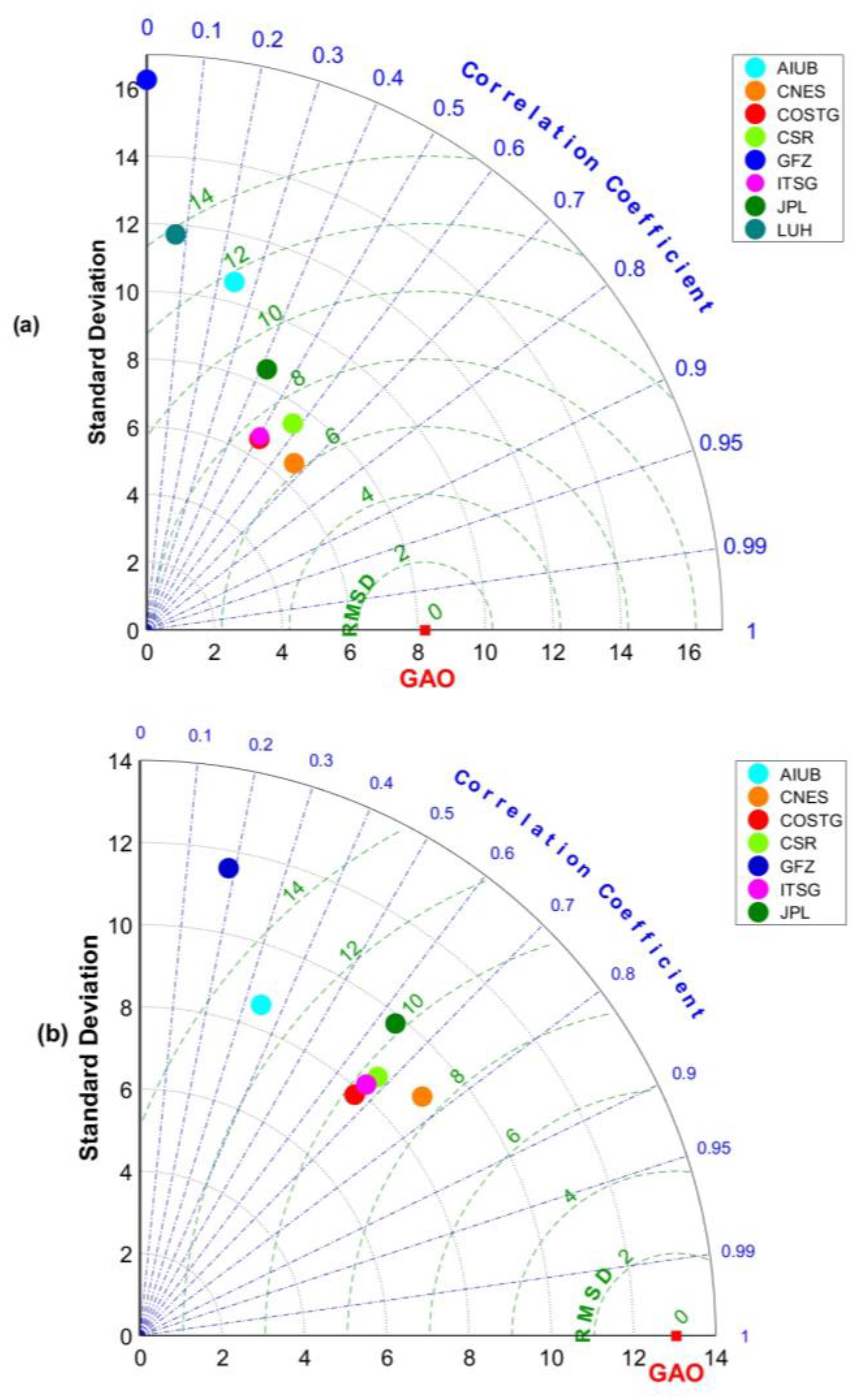
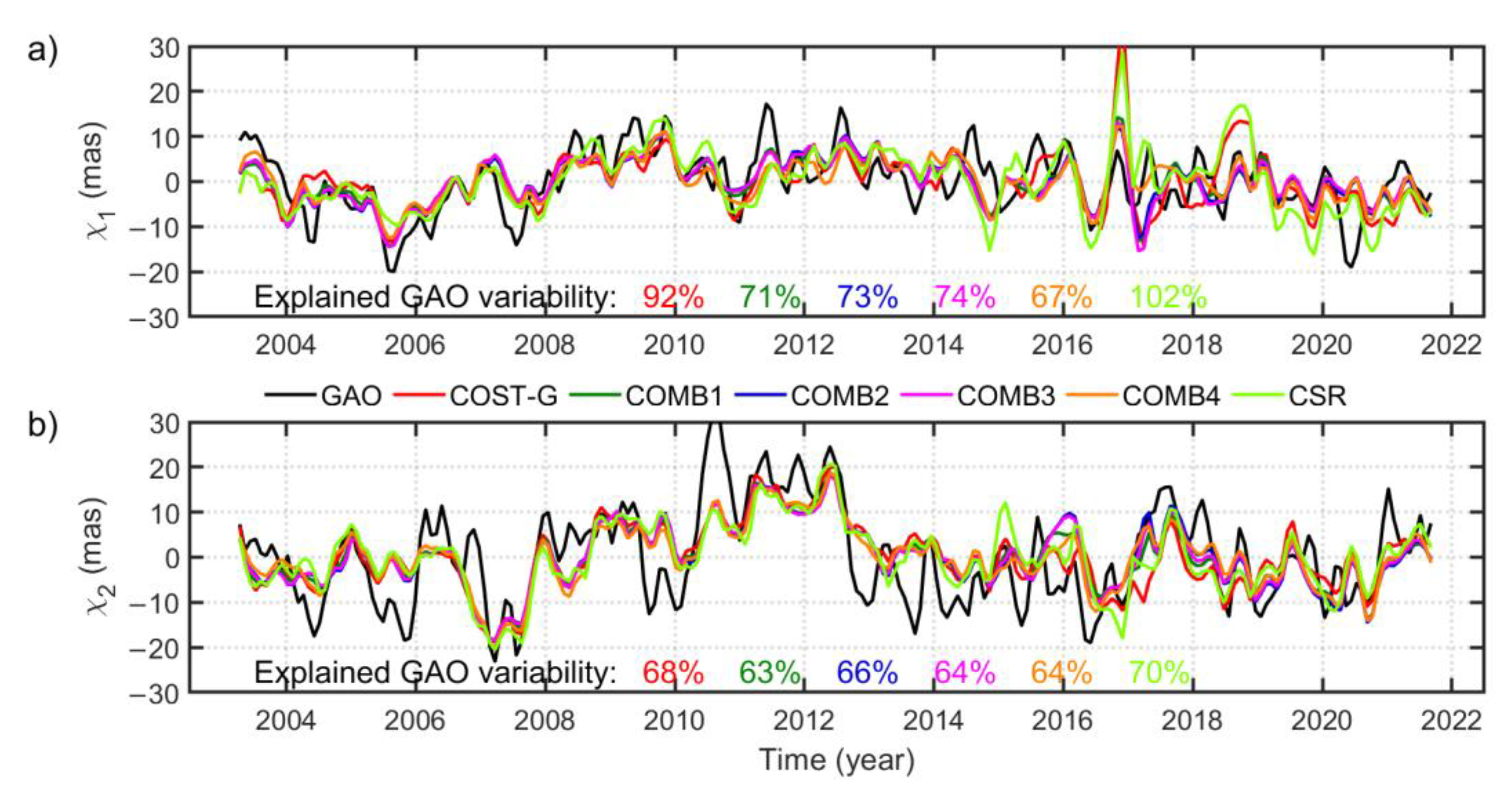
3.1. Overall Time Series

Before further processing, GAO and all gravimetric excitation series were filtered with a Gaussian filter to remove oscillations with periods shorter than one month and interpolated into the same moments of time for the period between April 2003 and September 2021 in order to maintain consistency in terms of data length and sampling. First, we study the overall variability of all detrended series (Figure 3). In contrast to the gravimetric excitation obtained from single GRACE/GRACE-FO solutions (Figure 1), all series based on combined data are relatively consistent with each other. However, they cannot fully represent the variability observed for GAO, especially in χ₂. In terms of the STD, all combined solutions (COMB1 to COMB4 and COST-G) explain 64% to 80% of GAO variability in the case of χ₁, whereas for χ₂ they can reconstruct 57% to 60% of GAO variability, depending on the solution (Figure 3). The notable peak in the COST-G and CSR time series for the χ₁ component around 2017 was probably caused by instrument issues at the end of the GRACE mission. The peak is not observed for GAO nor COMB solutions presented in this study, indicated that, in general, our method of combining gravimetric excitation series can reduce such artifacts. The χ₂ component is characterized by generally higher amplitudes than χ₁, which can be explained by the higher impact on land water mass variability on this component due to the spatial distribution of the main continents on the Northern Hemisphere [48].

In order to check the power of particular oscillations in the excitation series, we drew the amplitude spectra of complex-valued components of χ₁ + iχ₂ and consider their prograde (counter-clockwise) and retrograde (clockwise) parts (Figure 4). The spectra show that in both prograde and retrograde parts the strongest oscillation in GAO is annual, which confirms results from previous studies [5,6,19,20]. In the retrograde component, there are also prominent oscillations with periods of around 1100 and 550 days, while the prograde term exhibits variations with periods of about 180 (semiannual oscillation), 230, 500, and 560 days. The gravimetric excitation series replicates almost all oscillations detected in GAO but with noticeably smaller amplitudes. Of all considered series, excitations based on a single CSR solution reveal the highest amplitudes of each oscillation. It is worth noting that all COMB solutions are distinguished by smaller amplitudes than the solution with CSR, which is probably due to the removal of noise during the application of the TCH method. However, it is possible that this method removes some part of the real signal detected only by some individual GRACE/GRACE-FO solutions.

To analyse in detail the correspondence between GAO and each gravimetric excitation estimates, we present STD, zero-lag Corr, and RMSD of CSR, COST-G, and the COMB1 to COMB4-based series in a Taylor diagram (Figure 5). For the χ₁ component, all COMB solutions perform better than the single GRACE/GRACE-FO solution from CSR and the combined data provided by COST-G. For all series processed with the TCH method, RMSD values are between 5.80 and 6.19 mas, while Corr values are as high as 0.65–0.71. The better performance of COMB-based gravimetric excitation series than those from CSR and COST-G is replicated for the χ₂ component. The correlations with GAO are higher for χ₂ than for χ₁ as they exceed 0.70 for all COMB series. Nevertheless, RMSD values are less favourable than for χ₁ (between 9.08 and 9.43 mas for COMB series) because of the generally higher variability in the series for this component. For both equatorial components, the consistency between GAO and gravimetric excitation is highest for the COMB4 solution (combination of series from CSR, JPL, CNES, LUH, and AIUB), and lowest for the COST-G data. It should be noted that series based on a single CSR solution are characterized by the highest STD, which was also apparent in the time series plot (Figure 3).

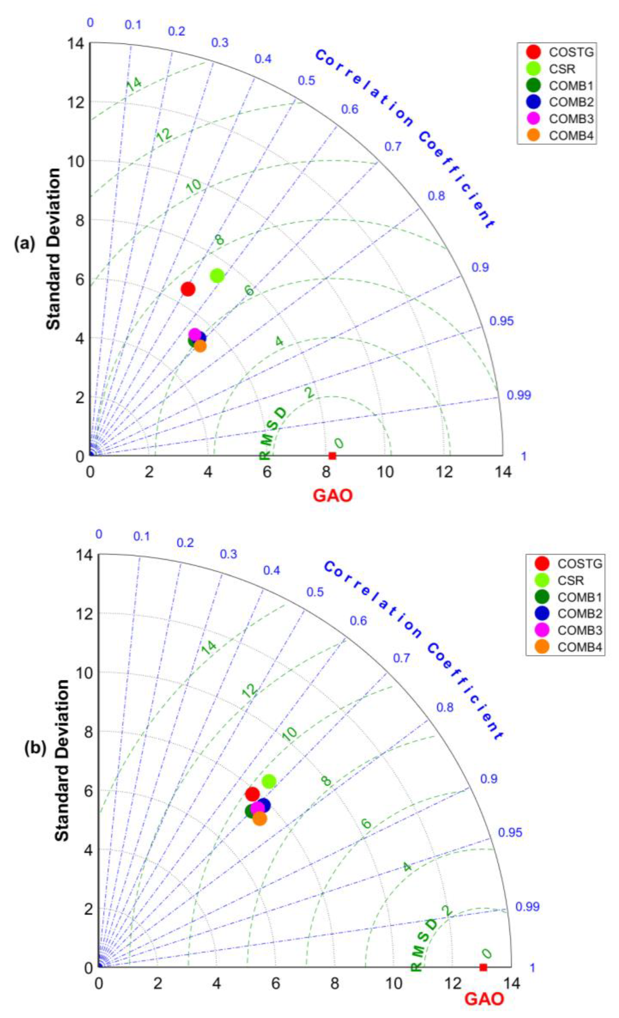
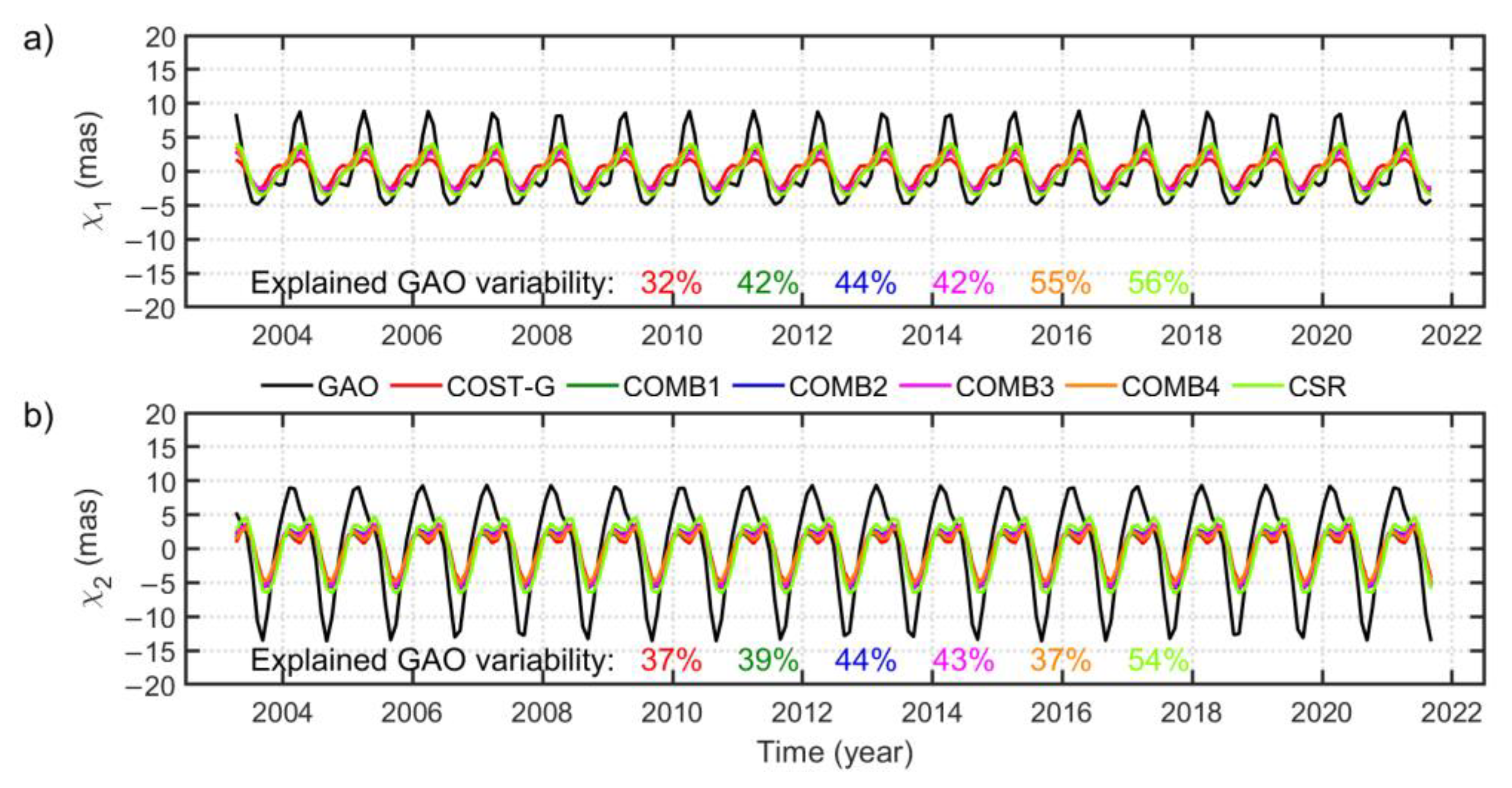
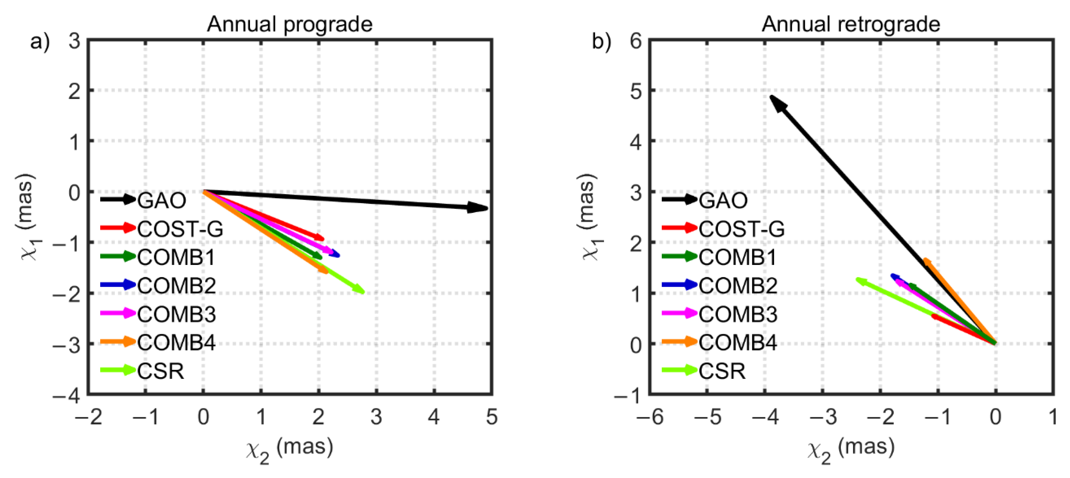
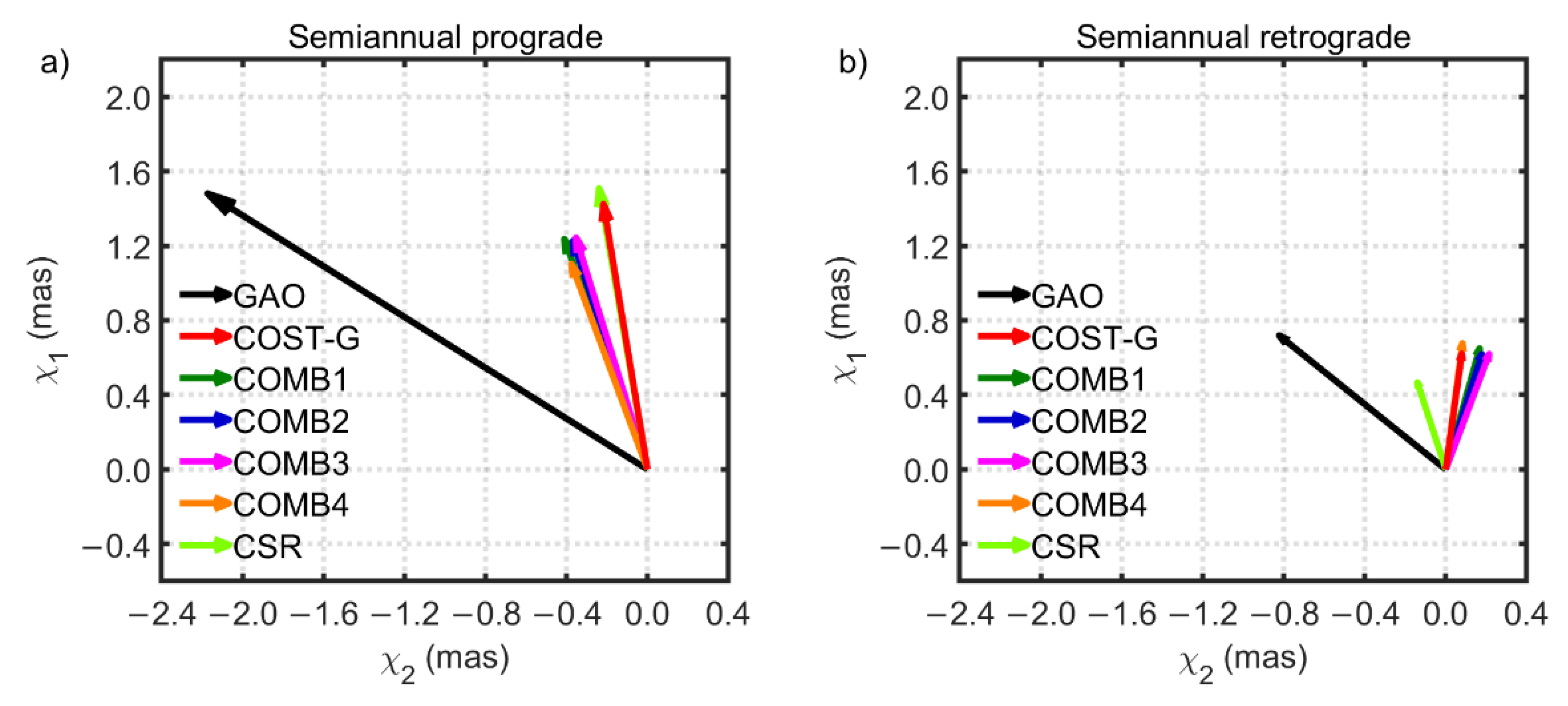
3.2. Seasonal Variations

We now extend our research to the analysis of seasonal oscillations in GAO and gravimetric excitation. Seasonal variations, apart from free Chandler wobble, are the most prominent oscillations in PM and are caused mainly by the mass distribution of the continental hydrosphere, atmosphere, and oceans [55]. Therefore, many previous studies focused on the analysis of these variations not only in observed GAM, but also in HAM, AAM, and OAM [5,6,17,26,29,48]. Here, we focus on seasonal changes in hydrological signal in geodetically observed PM excitation (GAO) and the same signal observed by GRACE/GRACE-FO and described with gravimetric excitation series. The analysed seasonal oscillations in PM excitation usually consist of annual, semiannual, and terannual variations.

Firstly, we draw seasonal series that were obtained by fitting three sinusoids (with the periods of 1, ½, and ⅓ year) to the overall detrended series with the use of the least-squares method (Figure 6). Figure 6 indicates that the seasonal variability is dominated by annual oscillation. All GRACE/GRACE-FO-based series are consistent with each other, but their amplitudes are visibly smaller than the amplitudes observed for GAO. This finding is consistent with the conclusions drawn on the basis of amplitude spectra analysis (Figure 4). All combined solutions explain 32% to 55% of GAO variability for χ₁, whereas for χ₂ they can reconstruct 37% to 44% of GAO variability, depending on the solution (Figure 6). The seasonal signal in PM excitation, mainly related to the seasonality of precipitation and related changes in soil water content, is generally stronger in the χ₂ component because of the higher dependence of this component on mass changes on the continents of the Northern Hemisphere.

Similar to the overall variability, we check the correspondence between GAO and each gravimetric excitation estimate in the seasonal spectral band by using Taylor diagrams (Figure 7). In general, the COMB solutions developed in this study are characterized by higher agreement with GAO than series based on COST-G data. For the χ₁ component, the RMSD values of the COMB-based series vary from 2.42 to 2.89 mas while the Corr values are between 0.89 and 0.91. For the χ₂ component, the corresponding values are between 4.69 and 5.10 mas for RMSD and between 0.85 and 0.89 for Corr. This confirms a good consistency among series developed with the TCH method. Gravimetric excitation determined from CSR data exhibits the lowest RMSD for both equatorial components of the PM excitation function, but the Corr values are consistent with those received for the COMB-based series.

To further study seasonal variations, we decomposed them into annual prograde, annual retrograde, semiannual prograde, and semiannual retrograde parts and show their amplitudes and phases (Figure 8 and Figure 9), which is a common approach for testing such oscillations [5,6,20,62]. Figure 8 demonstrates that for the observed hydrological signal in PM excitation (GAO), the retrograde component is characterized by higher amplitudes than for the prograde term, whereas for gravimetric excitations we observe the opposite situation. This characteristic is also nicely visualized in amplitude spectra (Figure 4). In general, all gravimetric excitation series underestimate annual amplitudes observed for GAO and these differences are more prominent for the retrograde term (Figure 8). The amplitude differences between GAO and COMB-based series are between 2.25 and 2.5 mas for the prograde term and between 3.99 and 4.35 mas for the retrograde term. Notably, COST-G-based series is characterized by the smallest amplitudes of annual oscillations, therefore, the use of this solution for the analysis of annual changes in PM excitation is not optimal. In terms of the phases of annual oscillation, all COMB-based series present relatively congruous results with phase differences with respect to GAO within 24–33° for the prograde term and 13–16° for the retrograde term (with the exception of the COMB4-based series, which is an almost perfect match for GAO in the annual retrograde term).

The similar phasor diagrams drawn for semiannual prograde and semiannual retrograde oscillations show that the semiannual retrograde variation is very weak for both GAO and gravimetric excitation (Figure 9). The results for COMB solutions are congruous; the amplitude differences with respect to GAO are between 1.33 and 1.47 mas for the prograde term and between 0.41 and 0.45 mas for the retrograde term, while the phase discrepancies are as high as 37–40° and 56–63° for the prograde and retrograde oscillation, respectively. Since the amplitudes of terannual oscillations turned out to be very small (Figure 4), they are not analysed in our study.

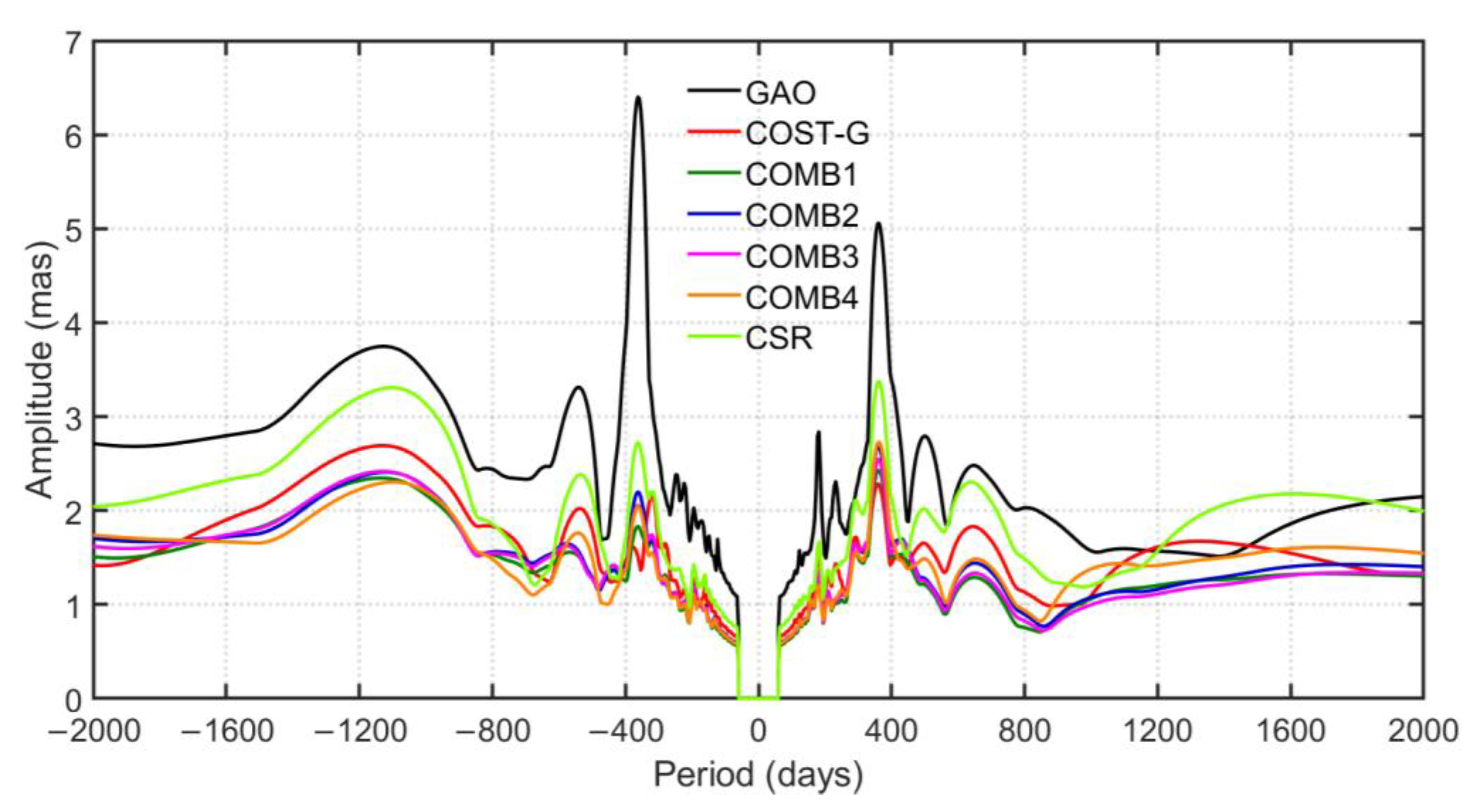
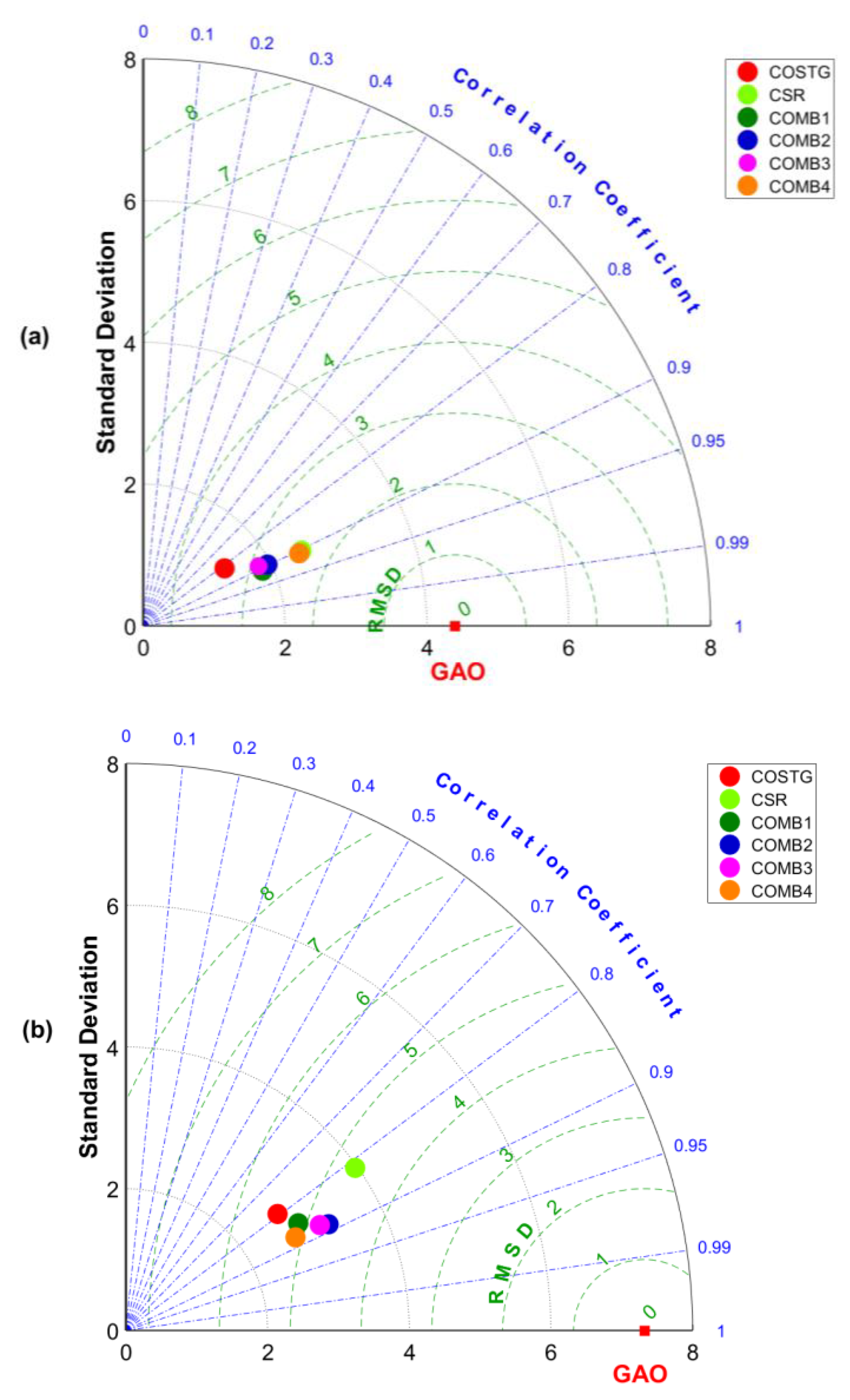
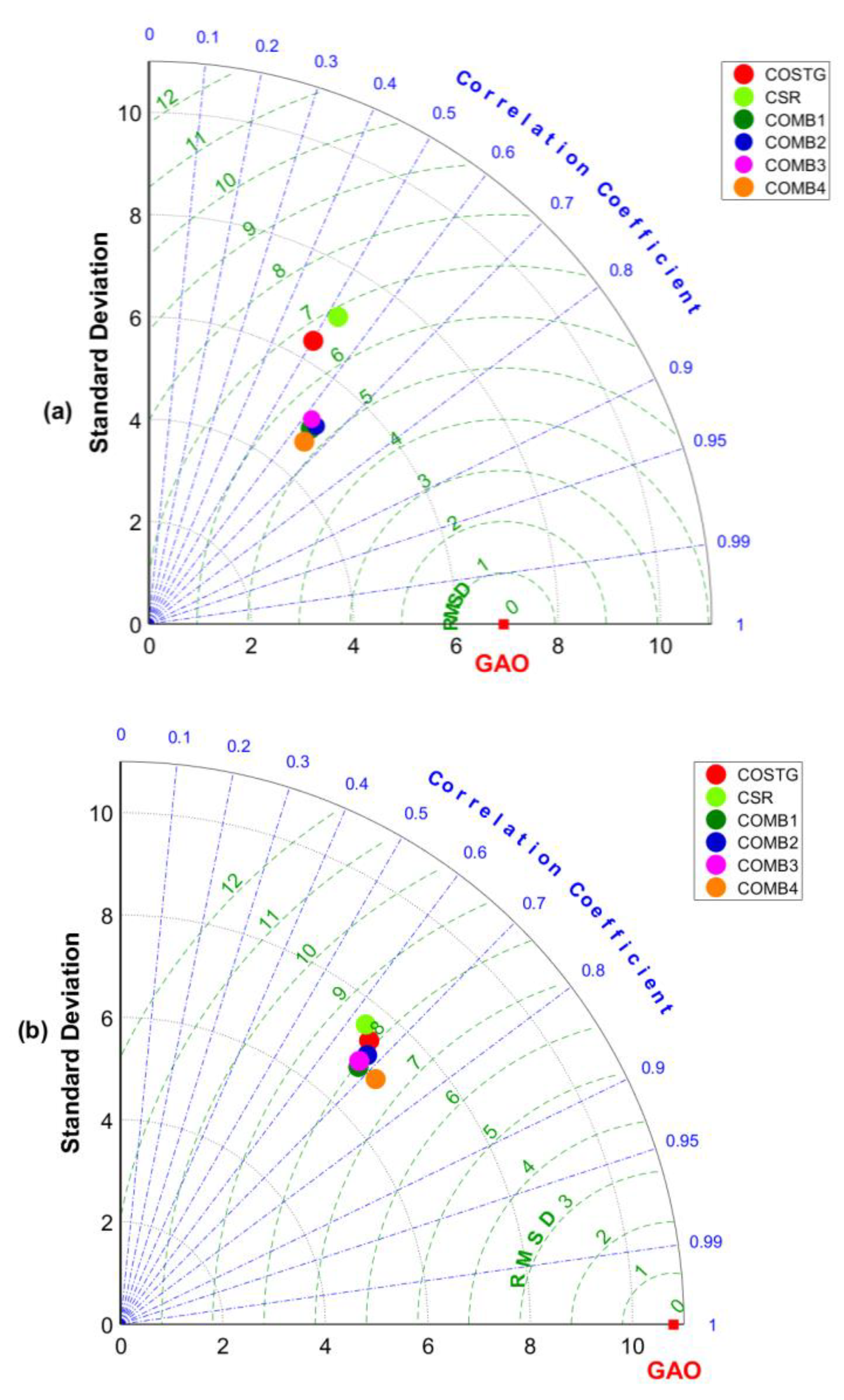
3.3. Nonseasonal Variations

All signals in PM excitation not captured by trends and seasonal variations should be reflected in residual series that are obtained after eliminating annual, semiannual, and terannual oscillations from the overall detrended series. Such variations are complex and consist of rapid (up to 100 days), interannual (500 days to 10 years), and decadal (above 10 years) changes [53]. These residual oscillations are denoted here as non-seasonal and are depicted in Figure 10, which indicates that despite excluding seasonal variations, the overall variability of residual series remains prominent. Removing seasonal signals reduced the differences in STD between the GAO and gravimetric excitation series. However, these discrepancies, especially in χ₂, are still apparent. For χ₁, all combined solutions explain 67% to 92% of the GAO variability, whereas for χ₂ they can reconstruct 63% to 68% of GAO variability, depending on the solution (Figure 10).

A thorough validation of gravimetric excitation series with the use of the parameters depicted in Figure 11 demonstrates that for non-seasonal variation, COMB-based series are characterized by a lower RMSD (between 5.27 and 5.48 mas for χ₁ and between 7.52 and 8.00 mas for χ₂) and higher Corr (between 0.62 and 0.65 for χ₁ and between 0.67 and 0.72 for χ₂) than the excitation series based on the CSR or COST-G solution. Therefore, the combined series processed with the TCH method can be generally recommended for use in PM excitation studies, especially in the non-seasonal spectral band. The COST-G- and CSR-based series present a similar level of consistency with GAO.

4. Discussion and Conclusions

In this study, we used the TCH method to determine four combined series of gravimetric excitation (COMB1 to COMB4), which are characterized by a minimal noise level. This was achieved by using a weighted mean of several single GRACE/GRACE-FO solutions, where the weights were inversely proportional to the noise level in every single solution.

Each of the four COMB series was determined with the use of different single GRACE/GRACE-FO solutions as the input but with the same solution (CSR RL06) treated as a reference in computations of noise in an individual series. We observed that the choice of weights calculated for each individual series with the use of the TCH method depends on the level of consistency with a chosen reference series. The lowest weights were assigned to the series characterized by the lowest agreement with the reference series, whereas the highest weights were computed for the series characterized by the highest consistency with the reference.

Despite differences in input single solutions and assigned weights, all COMB series were consistent with each other and presented a similar level of consistency with GAO. The COMB4 (weighted mean of CNES, JPL, CSR, LUH, and AIUB) performed only slightly better than the other COMB series for overall and non-seasonal variation. The series based on single GRACE/GRACE-FO solutions were not as consistent with each other as the COMB series and presented a range of levels of agreement with GAO. We also observed that series based on GFZ, LUH, and AIUB showed the highest variation from the other solutions. In addition, most of the single solutions provided a lower level of consistency with GAO than the COMB series.

The application of the TCH method minimized noise in the time series, hence COMB-based gravimetric excitation series were slightly smoothed and were characterized by lower variability (as described with STD values) than series based on single GRACE/GRACE-FO solutions. However, it is possible that a part of the real signal detected only by some of the individual solutions was removed when combining series with the TCH method.

The obtained level of consistency between COMB-based gravimetric excitation series and GAO was as follows. For overall variability, the Corr values were between 0.65 and 0.71 for χ₁ and between 0.70 and 0.74 for χ₂, while the RMSD varied from 5.80 to 6.19 mas for χ₁ and from 9.08 to 9.43 mas for χ₂. For seasonal oscillations, the Corr values ranged from 0.89 to 0.91 for χ₁ and from 0.85 to 0.89 for χ₂, while RMSD values were as high as 2.42 to 2.89 mas for χ₁ and 4.69 to 5.10 mas for χ₂. For non-seasonal variation, the Corr values were between 0.62 and 0.65 for χ₁ and between 0.67 and 0.72 for χ₂ while RMSD values were between 5.27 and 5.48 mas for χ₁ and between 7.52 and 8.00 mas for χ₂. These findings confirm that seasonal variations in PM excitation are better determined by GRACE/GRACE-FO than non-seasonal variations, which is consistent with findings from our previous research [20,23,24].

A comparison of results from COMB with those from the combined solution provided by COST-G showed that our combinations, which are computed on the level of gravimetric excitation series, provide higher consistency with GAO than the COST-G solution, which is a combination performed on the level of SH coefficients of geopotential. The corresponding values of Corr and RMSD for COST-G series were as follows. For overall variability, the Corr values were as high as 0.51 for χ₁ and 0.67 for χ₂ while RMSD was 7.45 and 9.76 for χ₁ and χ₂, respectively. For seasonal oscillations, the Corr values were as high as 0.82 for χ₁ and 0.79 for χ₂ while RMSD was 3.34 and 5.42 for χ₁ and χ₂, respectively. For non-seasonal variation, the Corr values were as high as 0.50 for χ₁ and 0.66 for χ₂, while RMSD was 6.66 and 8.11 for χ₁ and χ₂, respectively.

Although the COMB solutions gave more satisfactory results than the COST-G solution for all analysed oscillations, we noticed that in terms of seasonal variations, results from a single CSR solution were comparable to those received for the COMB series (the Corr values were equal to 0.90 for χ₁ and 0.82 for χ₂ while RMSD values were equal to 2.40 for χ₁ and 4.67 for χ₂). Therefore, it can be concluded that the combinations based on minimizing the noise level (COMB) are particularly useful for both the overall time series and for non-seasonal variations.

It should be kept in mind that our method of developing combined gravimetric excitation series is not based on minimizing differences with respect to GAO but on reducing the noise level in the series, where the noise is determined by comparing several gravimetric excitation series. This means that no external reference data are used in this combination. There is still room for improvement by combining data from GRACE and GRACE-FO with other datasets (e.g., SLR), as we obtained relatively high agreement between GAO and the gravimetric excitation series based on the CNES solution. Potential combination with other datasets, such as solutions based on high-low satellite-to-satellite tracking of Swarm satellites, is also worth exploring.

References

1. Barnes, R.T.H.; Hide, R.; White, A.; Wilson, C.A. Atmospheric angular momentum fluctuations, length-of-day changes and polar motion. Proc. R. Soc. A 1983, 387, 31–73. [Google Scholar] [CrossRef]
2. Lambeck, K. The Earth’s Variable Rotation: Geophysical Causes and Consequences (Cambridge Monographs on Mechanics); Cambridge University Press: Cambridge, UK, 1980. [Google Scholar] [CrossRef]
3. Adhikari, S.; Ivins, E.R. Climate-driven polar motion: 2003–2015. Sci. Adv. 2016, 2, e1501693. [Google Scholar] [CrossRef] [PubMed] [Green Version]
4. Brzeziński, A.; Ponte, R.M.; Ali, A.H. Non-tidal oceanic excitation of nutation and diurnal/semi-diurnal polar motion revisited. J. Geophys. Res. Solid Earth 2004, 109, 1–14. [Google Scholar] [CrossRef] [Green Version]
5. Brzeziński, A.; Nastula, J.; Kołaczek, B. Seasonal excitation of polar motion estimated from recent geophysical models and observations. J. Geodyn. 2009, 48, 235–240. [Google Scholar] [CrossRef] [Green Version]
6. Dobslaw, H.; Dill, R.; Grötzsch, A.; Brzeziński, A.; Thomas, M. Seasonal polar motion excitation from numerical models of atmosphere, ocean, and continental hydrosphere. J. Geophys. Res. Solid Earth 2010, 115, 1–11. [Google Scholar] [CrossRef] [Green Version]
7. Göttl, F.; Schmidt, M.; Seitz, F. Mass-related excitation of polar motion: An assessment of the new RL06 GRACE gravity field models. Earth Planets Space 2018, 70, 195. [Google Scholar] [CrossRef] [Green Version]
8. Gross, R.S.; Fukumori, I.; Menemenlis, D. Atmospheric and oceanic excitation of the Earth’s wobbles during 1980–2000. J. Geophys. Res. 2003, 108. [Google Scholar] [CrossRef] [Green Version]
9. Gross, R.S.; Fukumori, I.; Menemenlis, D.; Gegout, P. Atmospheric and oceanic excitation of length-of-day variations during 1980–2000. J. Geophys. Res. Solid Earth 2004, 109, B01406. [Google Scholar] [CrossRef]
10. Jin, S.; Chambers, D.P.; Tapley, B.D. Hydrological and oceanic effects on polar motion from GRACE and models. J. Geophys. Res. Solid Earth 2010, 115, 1–11. [Google Scholar] [CrossRef]
11. Nastula, J.; Wińska, M.; Śliwińska, J.; Salstein, D. Hydrological signals in polar motion excitation—Evidence after fifteen years of the GRACE mission. J. Geodyn. 2019, 124, 119–132. [Google Scholar] [CrossRef]
12. Seoane, L.; Biancale, R.; Gambis, D. Agreement between Earth’s rotation and mass displacement as detected by GRACE. J. Geodyn. 2012, 62, 49–55. [Google Scholar] [CrossRef]
13. Kornfeld, R.P.; Arnold, B.W.; Gross, M.A.; Dahya, N.T.; Klipstein, W.M. GRACE-FO: The Gravity Recovery and Climate Experiment Follow-On Mission. J. Spacecr. Rocket. 2019, 56, 931–951. [Google Scholar] [CrossRef]
14. Tapley, B.D.; Bettadpur, S.; Watkins, M.; Reigber, C. The gravity recovery and climate experiment: Mission overview and early results. Geophys. Res. Lett. 2004, 31, L09607. [Google Scholar] [CrossRef] [Green Version]
15. Chen, J.L.; Wilson, C.R. Low degree gravity changes from GRACE, earth rotation, geophysical models and satellite laser ranging. J. Geophys. Res. Solid Earth 2008, 113, 1–9. [Google Scholar] [CrossRef] [Green Version]
16. Cheng, M.; Ries, J.C.; Tapley, B.D. Variations of the Earth’s figure axis from Satellite Laser Ranging and GRACE. J. Geophys. Res. Solid Earth 2011, 116, 1–14. [Google Scholar] [CrossRef] [Green Version]
17. Nastula, J.; Pasnicka, M.; Kolaczek, B. Comparison of the geophysical excitations of polar motion from the period 1980.0–2007.0. Acta Geophys. 2011, 59, 561–577. [Google Scholar] [CrossRef]
18. Nastula, J.; Śliwińska, J. Prograde and retrograde terms of gravimetric polar motion excitation estimates from the GRACE monthly gravity field models. Remote Sens. 2020, 12, 138. [Google Scholar] [CrossRef] [Green Version]
19. Seoane, L.; Nastula, J.; Bizouard, C.; Gambis, D. The use of gravimetric data from GRACE mission in the understanding of polar motion variations. Geophys. J. Int. 2009, 178, 614–622. [Google Scholar] [CrossRef] [Green Version]
20. Śliwińska, J.; Nastula, J.; Dobslaw, H.; Dill, R. Evaluating gravimetric polar motion excitation estimates from the RL06 GRACE monthly-mean gravity field models. Remote Sens. 2020, 12, 930. [Google Scholar] [CrossRef]
21. Meyrath, T.; van Dam, T. A comparison of interannual hydrological polar motion excitation from GRACE and geodetic observations. J. Geodyn. 2016, 99, 1–9. [Google Scholar] [CrossRef]
22. Śliwińska, J.; Wińska, M.; Nastula, J. Preliminary estimation and validation of polar motion excitation from different types of the grace and grace follow-on missions data. Remote Sens. 2020, 12, 3490. [Google Scholar] [CrossRef]
23. Śliwińska, J.; Nastula, J.; Wińska, M. Evaluation of hydrological and cryospheric angular momentum estimates based on GRACE, GRACE-FO and SLR data for their contributions to polar motion excitation. Earth Planets Space 2021, 73, 71. [Google Scholar] [CrossRef]
24. Śliwińska, J.; Wińska, M.; Nastula, J. Validation of GRACE and GRACE-FO Mascon Data for the Study of Polar Motion Excitation. Remote Sens. 2021, 13, 1152. [Google Scholar] [CrossRef]
25. Nastula, J.; Ponte, R.M.; Salstein, D.A. Comparison of polar motion excitation series derived from GRACE and from analyses of geophysical fluids. Geophys. Res. Lett. 2007, 34. [Google Scholar] [CrossRef]
26. Seoane, L.; Nastula, J.; Bizouard, C.; Gambis, D. Hydrological excitation of polar motion derived from GRACE gravity field solutions. Int. J. Geophys. 2011, 2011, 174396. [Google Scholar] [CrossRef]
27. Śliwińska, J.; Wińska, M.; Nastula, J. Terrestrial water storage variations and their effect on polar motion. Acta Geophys. 2019, 67, 17–39. [Google Scholar] [CrossRef] [Green Version]
28. Wińska, M.; Nastula, J.; Kołaczek, B. Assessment of the global and regional land hydrosphere and its impact on the balance of the geophysical excitation function of polar motion. Acta Geophys. 2016, 64, 270–292. [Google Scholar] [CrossRef] [Green Version]
29. Wińska, M.; Nastula, J.; Salstein, D.A. Hydrological excitation of polar motion by different variables from the GLDAS model. J. Geod. 2017, 91, 1461–1473. [Google Scholar] [CrossRef] [Green Version]
30. Jean, Y.; Meyer, U.; Jäggi, A. Combination of GRACE monthly gravity field solutions from different processing strategies. J. Geod. 2018, 92, 1313–1328. [Google Scholar] [CrossRef]
31. Meyer, U.; Jean, Y.; Kvas, A.; Dahle, C.; Lemoine, J.M.; Jäggi, A. Combination of GRACE monthly gravity fields on the normal equation level. J. Geod. 2019, 93, 1645–1658. [Google Scholar] [CrossRef] [Green Version]
32. Jäggi, A.; Meyer, U.; Lasser, M.; Jenny, B.; Lopez, T.; Flechtner, F.; Dahle, C.; Förste, C.; Mayer-Gürr, T.; Kvas, A.; et al. International Combination Service for Time-Variable Gravity Fields (COST-G). Int. Assoc. Geod. Symp. 2019, 152, 57–65. [Google Scholar] [CrossRef]
33. Encarnacao, J.; Visser, P.; Jaeggi, A.; Bezdek, A.; Mayer-Gürr, T.; Shum, C.K.; Arnold, D.; Doornbos, E.; Elmer, M.; Guo, J.; et al. Multi-Approach Gravity Field Models from Swarm GPS Data; GFZ Data Services: Potsdam, Germany, 2019. [Google Scholar] [CrossRef]
34. Lemoine, J.-M.; Biancale, R.; Reinquin, F.; Bourgogne, S.; Gégout, P. CNES/GRGS RL04 Earth Gravity Field Models, from GRACE and SLR Data; GFZ Data Services: Potsdam, Germany, 2019. [Google Scholar] [CrossRef]
35. Meyer, U.; Sosnica, K.; Arnold, D.; Dahle, C.; Thaller, D.; Dach, R.; Jäggi, A. SLR, GRACE and Swarm Gravity Field Determination and Combination. Remote Sens. 2019, 11, 956. [Google Scholar] [CrossRef] [Green Version]
36. Weigelt, M. Time Series of Monthly Combined HLSST and SLR Gravity Field Models to Bridge the Gap between GRACE and GRACE-FO: QuantumFrontiers_HLSST_SLR_COMB2019s; GFZ Data Services: Potsdam, Germany, 2019. [Google Scholar] [CrossRef]
37. Sasgen, I.; Martinec, Z.; Fleming, K. Wiener optimal combination and evaluation of the Gravity Recovery and Climate Experiment (GRACE) gravity fields over Antarctica. J. Geophys. Res. Solid Earth 2007, 112, B04401. [Google Scholar] [CrossRef] [Green Version]
38. Sakumura, C.; Bettadpur, S.; Bruinsma, S. Ensemble prediction and intercomparison analysis of GRACE time-variable gravity field models. Geophys. Res. Lett. 2014, 41, 1389–1397. [Google Scholar] [CrossRef]
39. Śliwińska, J.; Birylo, M.; Rzepecka, Z.; Nastula, J. Analysis of groundwater and total water storage changes in Poland using GRACE observations, in-situ data, and various assimilation and climate models. Remote Sens. 2019, 11, 2949. [Google Scholar] [CrossRef]
40. Premoli, A.; Tavella, P. A revisited three-cornered hat method for estimating frequency standard instability. IEEE Trans. Instrum. Meas. 1993, 42, 7–13. [Google Scholar] [CrossRef]
41. Koot, L.; de Viron, O.; Dehant, V. Atmospheric angular momentum time-series: Characterization of their internal noise and creation of a combined series. J. Geod. 2006, 79, 663–674. [Google Scholar] [CrossRef]
42. Quinn, K.J.; Ponte, R.M.; Heimbach, P.; Fukumori, I.; Campin, J.-M. Ocean angular momentum from a recent global state estimate, with assessment of uncertainties. Geophys. J. Int. 2019, 216, 584–597. [Google Scholar] [CrossRef]
43. Vernotte, F.; Addouche, M.; Delporte, M.; Brunet, M. The three cornered hat method: An attempt to identify some clock correlations. In Proceedings of the 2004 IEEE International Frequency Control Symposium and Exposition, Montreal, QC, Canada, 23–27 August 2004; pp. 482–488. [Google Scholar] [CrossRef]
44. O’Carroll, A.G.; Eyre, J.R.; Saunders, R.W. Three-way error analysis between AATSR, AMSR-E, and in situ sea surface temperature observations. J. Atmos. Ocean. Technol. 2008, 25, 1197–1207. [Google Scholar] [CrossRef] [Green Version]
45. Sjoberg, J.P.; Anthes, R.A.; Rieckh, T. The Three-Cornered Hat Method for Estimating Error Variances of Three or More Atmospheric Datasets. Part I: Overview and Evaluation. J. Atmos. Ocean. Technol. 2021, 38, 555–572. [Google Scholar] [CrossRef]
46. Roebeling, R.A.; Wolters EL, A.; Meirink, J.F.; Leijnse, H. Triple collocation of summer precipitation retrievals from SEVIRI over Europe with gridded rain gauge and weather radar data. J. Hydrometeor. 2012, 13, 1552–1566. [Google Scholar] [CrossRef]
47. Nastula, J.; Śliwińska, J.; Kur, T.; Wińska, M.; Partyka, A. Preliminary study on hydrological angular momentum determined from CMIP6 historical simulations. Earth Planets Space 2022, 74, 84. [Google Scholar] [CrossRef]
48. Chen, J.L.; Wilson, C.R.; Zhou, Y.H. Seasonal excitation of polar motion. J. Geodyn. 2012, 62, 8–15. [Google Scholar] [CrossRef]
49. Wińska, M.; Śliwińska, J. Assessing hydrological signal in polar motion from observations and geophysical models. Stud Geophys Geod 2019, 63, 95–117. [Google Scholar] [CrossRef]
50. Naito, I.; Zhou, Y.H.; Sugi, M.; Kawamura, R.; Sato, N. Three-dimensional atmospheric angular momentum simulated by the Japan Meteorological Agency model for the period of 1955–1994. J. Meteorol. Soc. Jpn. Ser. II 2000, 78, 111–122. [Google Scholar] [CrossRef]
51. Zhou, Y.H.; Chen, J.L.; Liao, X.H.; Wilson, C.R. Oceanic excitations on polar motion: A cross comparison among models. Geophys. J. Int. 2005, 162, 390–398. [Google Scholar] [CrossRef] [Green Version]
52. Chen, W.; Li, J.; Ray, J.; Cheng, M. Improved Geophysical Excitations Constrained by Polar Motion Observations and GRACE/SLR Time-Dependent Gravity. Geod. Geodyn. 2017, 8, 377–388. [Google Scholar] [CrossRef]
53. Bizouard, C. Geophysical Modelling of the Polar Motion; De Gruyter: Berlin, Germany; Boston, MA, USA, 2020. [Google Scholar] [CrossRef]
54. Bizouard, C.; Lambert, S.; Gattano, C.; Becker, O.; Richard, J.-Y. The IERS EOP 14C04 solution for Earth orientation parameters consistent with ITRF 2014. J. Geod. 2019, 93, 621–633. [Google Scholar] [CrossRef]
55. Gross, R. Theory of Earth Rotation Variations. In VIII Hotine-Marussi Symposium on Mathematical Geodesy; Sneeuw, N., Novák, P., Crespi, M., Sansò, F., Eds.; Springer: Cham, Switzerland, 2015. [Google Scholar] [CrossRef]
56. Wilson, C.R.; Vicente, R.O. Maximum likelihood estimates of polar motion parameters. In Variations in Earth Rotation; McCarthy, D.D., Carter, W.E., Eds.; AGU Geophysical Monograph Series; Wiley: Washington, DC, USA, 1990; Volume 59, pp. 151–155. [Google Scholar]
57. Nastula, J.; Gross, R. Chandler wobble parameters from SLR and GRACE. J. Geophys. Res. Solid Earth 2015, 120, 4474–4483. [Google Scholar] [CrossRef]
58. Available online: https://hpiers.obspm.fr/eop-pc/index.php?index=excitactive&lang=en (accessed on 1 July 2022).
59. Dill, R.; Dobslaw, H.; Hellmers, H.; Kehm, A.; Bloßfeld, M.; Thomas, M.; Seitz, F.; Thaller, D.; Hugentobler, U.; Schönemann, E. Evaluating processing choices for the geodetic estimation of Earth orientation parameters with numerical models of global geophysical fluids. J. Geophys. Res. Solid Earth 2020, 125, e2020JB020025. [Google Scholar] [CrossRef]
60. Dobslaw, H.; Dill, R. Effective Angular Momentum Functions From Earth System Modelling at GeoForschungsZentrum in Potsdam; Technical Report, Revision 1.0; GFZ: Potsdam, Germany, 2018; Available online: ftp://ig2-dmz.gfz-potsdam.de/EAM/ESMGFZ_EAM_Product_Description_Document.pdf (accessed on 1 July 2022).
61. Yu, N.; Ray, J.; Li, J.; Chen, G.; Chao, N.; Chen, W. Intraseasonal variations in atmospheric and oceanic excitation of length-of-day. Earth Space Sci. 2021, 8, e2020EA001563. [Google Scholar] [CrossRef]
62. Jungclaus, J.H.; Fischer, N.; Haak, H.; Lohmann, K.; Marotzke, J.; Matei, D.; Mikolajewicz, U.; Notz, D.; von Storch, J.S. Characteristics of the ocean simulations in MPIOM, the ocean component of the MPI-Earth system model. J. Adv. Model. Earth Syst. 2013, 5, 422–446. [Google Scholar] [CrossRef]
63. Dill, R.; Dobslaw, H. Seasonal variations in global mean sea level and consequences on the excitation of length-of-day changes. Geophys. J. Int. 2019, 218, 801–816. [Google Scholar] [CrossRef]
64. Chen, W.; Shen, W. New estimates of the inertia tensor and rotation of the triaxial nonrigid Earth. J. Geophys. Res. 2010, 115, B12419. [Google Scholar] [CrossRef]
65. Box, G.E.P.; Jenkins, G.M.; Reinsel, G.C.; Ljung, G.M. Time Series Analysis: Forecasting and Control, 5th ed.; John Wiley and Sons Inc.: Hoboken, NJ, USA, 2016; ISBN 978-1-118-67502-1. [Google Scholar]
66. Koch, I.; Flury, J.; Naeimi, M.; Shabanloui, A. LUH-GRACE2018: A New Time Series of Monthly Gravity Field Solutions from GRACE. In International Association of Geodesy Symposia; Springer: Berlin/Heidelberg, Germany, 2020. [Google Scholar] [CrossRef] [Green Version]
67. Meyer, U.; Jäggi, A.; Jean, Y.; Beutler, G. AIUB-RL02: An improved time-series of monthly gravity fields from GRACE data. Geophys. J. Int. 2016, 205, 1196–1207. [Google Scholar] [CrossRef] [Green Version]
68. Dahle, C.; Murböck, M.; Flechtner, F.; Dobslaw, H.; Michalak, G.; Neumayer, K.H.; Abrykosov, O.; Reinhold, A.; König, R.; Sulzbach, R.; et al. The GFZ GRACE RL06 monthly gravity field time series: Processing details and quality assessment. Remote Sens. 2019, 11, 2116. [Google Scholar] [CrossRef] [Green Version]
69. Taylor, K.E. Summarizing multiple aspects of model performance in a single diagram. J. Geophys. Res. 2001, 106, 7183–7192. [Google Scholar] [CrossRef]
70. Gray, J.E.; Allan, D.W. A method for estimating the frequency stability of an individual oscillator. In Proceedings of the 28th Annual Symposium on Frequency Control, Atlantic City, NJ, USA, 29–31 May 1974; pp. 243–246. [Google Scholar] [CrossRef] [Green Version]
71. Chin, T.; Gross, R.; Dickey, J. Multi-reference evaluation of uncertainty in earth orientation parameter measurements. J. Geod. 2005, 79, 24–32. [Google Scholar] [CrossRef]
72. Ferreira, V.G.; Montecino, H.D.C.; Yakubu, C.I.; Heck, B. Uncertainties of the Gravity Recovery and Climate Experiment time-variable gravity-field solutions based on three-cornered hat method. J. Appl. Rem. Sens. 2016, 10, 015015. [Google Scholar] [CrossRef]
73. Grubbs, F.E. On Estimating Precision of Measuring Instruments and Product Variability. J. Am. Stat. Assoc. 1948, 43, 243–264. [Google Scholar] [CrossRef]
74. Torcaso, F.; Ekstrom, C.R.; Burt, E.; Matsaki, D. Estimating Frequency Stability and Cross-Correlations. In Proceedings of the 30th Annual Precise Time and Time Interval Systems and Applications Meeting, Reston, VA, USA, 1–3 December 1998; pp. 69–82. [Google Scholar]
Figure 1. Time series of χ1 (a) and χ2 (b) components of GAO, gravimetric excitation determined from seven GRACE/GRACE-FO single solutions (CSR, JPL, GFZ, ITSG, CNES, AIUB, and LUH) and one combined solution (COST-G) after filling a near-year data gap between the end of GRACE and the start of the GRACE-FO operation. The series were filtered using a Gaussian filter with full width at half maximum (FWHM) equal to 60 days. The linear trends determined with the use of the least-squares method were removed from the series.
Remotesensing 14 06292 g001
Figure 2. Taylor diagrams showing a comparison of χ1 (a), and χ2 (b) components of GAO (treated as a reference value), with gravimetric PM excitation determined from seven GRACE/GRACE-FO single solutions (CSR, JPL, GFZ, ITSG, CNES, AIUB, and LUH) and one combined solution (COST-G). The critical value of the correlation coefficient for 75 independent points and a 95% confidence level is 0.19, and the standard error of the difference between the two correlation coefficients is 0.17.
Remotesensing 14 06292 g002
Figure 3. Time series of χ1 (a) and χ2 (b) components of GAO and gravimetric excitation determined from a single GRACE/GRACE-FO solution (CSR), combined GRACE/GRACE-FO solution (COST-G), and the four combined solutions developed in this study (COMB1, COMB2, COMB3, and COMB4). The plots include values of explained GAO variability, which was computed as a relation between STD of gravimetric excitation and STD of GAO (STDgravimetric excitation/STDGAO) given in %.
Remotesensing 14 06292 g003
Figure 4. Amplitude spectra of the GAO and gravimetric excitation series determined from the single GRACE/GRACE-FO solution (CSR), combined GRACE/GRACE-FO solution (COST-G), and the four combined solutions developed in this study (COMB1, COMB2, COMB3, and COMB4). The spectra were computed in a broadband with a 60–2000-day cut-off. The plus time period on the plot indicates a prograde term and minus time period indicates a retrograde term. Note that periods shorter than 60 days are not considered as the series were sampled monthly and their Nyquist frequency is about 6 cycles per year, which corresponds to periods of about 60 days.
Remotesensing 14 06292 g004
Figure 5. Taylor diagrams showing a comparison of χ1 (a) and χ2 (b) components of GAO (treated as a reference value), with gravimetric excitation determined from a single GRACE/GRACE-FO solution (CSR), combined GRACE/GRACE-FO solution (COST-G), and the four combined solutions developed in this study (COMB1, COMB2, COMB3, and COMB4). The critical value of the correlation coefficient for 75 independent points and a 95% confidence level is 0.19, and the standard error of the difference between the two correlation coefficients is 0.17.
Remotesensing 14 06292 g005
Figure 6. Time series of seasonal χ1 (a) and χ2 (b) components of GAO and gravimetric excitation determined from a single GRACE/GRACE-FO solution (CSR), combined GRACE/GRACE-FO solution (COST-G), and the four combined solutions developed in this study (COMB1, COMB2, COMB3, and COMB4). The plots include values of explained GAO variability, which was computed as a relation between STD of gravimetric excitation and STD of GAO (STDgravimetric excitation/STDGAO) given in %.
Remotesensing 14 06292 g006
Figure 7. Taylor diagrams showing a comparison of seasonal χ1 (a) and χ2 (b) components of GAO (treated as a reference) with gravimetric excitation determined from a single GRACE/GRACE-FO solution (CSR), combined GRACE/GRACE-FO solution (COST-G), and the four combined solutions developed in this study (COMB1, COMB2, COMB3, and COMB4). The critical value of the correlation coefficient for seasonal variation for 90 independent points and a 95% confidence level is 0.17, and the standard error of the difference between the two correlation coefficients is 0.15.
Remotesensing 14 06292 g007
Figure 8. Phasor diagrams of the annual prograde (a) and annual retrograde (b) variation in complex series (χ1 + iχ2) of gravimetric excitation and GAO. Phase (φ) is defined by the annual term as sin(2π(t − t0) + φ), where t0 is the reference epoch (1 January 2004).
Remotesensing 14 06292 g008
Figure 9. Phasor diagrams of semiannual prograde (a) and semiannual retrograde (b) variation in complex series (χ1 + iχ2) of gravimetric excitation and GAO. Phase (φ) is defined by the semiannual term as sin(4π(t − t0) + φ), where t0 is the reference epoch (1 January 2004).
Remotesensing 14 06292 g009
Figure 10. Time series of non-seasonal χ1 (a) and χ2 (b) components of GAO and gravimetric excitation determined from a single GRACE/GRACE-FO solution (CSR), combined GRACE/GRACE-FO solution (COST-G), and the four combined solutions developed in this study (COMB1, COMB2, COMB3, and COMB4). The plots include values of explained GAO variability, which was computed as a relation between STD of gravimetric excitation and STD of GAO (STDgravimetric excitation/STDGAO) given in %.
Remotesensing 14 06292 g010
Figure 11. Taylor diagrams showing a comparison of non-seasonal χ1 (a) and χ2 (b) components of GAO (treated as a reference) with gravimetric excitation determined from a single GRACE/GRACE-FO solution (CSR), combined GRACE/GRACE-FO solution (COST-G), and the four combined solutions developed in this study (COMB1, COMB2, COMB3, and COMB4). The critical value of the correlation coefficient for non-seasonal variation for 55 independent points and a 95% confidence level is 0.22, and the standard error of the difference between the two correlation coefficients is 0.20.
Remotesensing 14 06292 g011