Abstract
After exploratory research in the 1950s, HF skywave ‘over-the-horizon’ radars (OTHR) were developed as operating systems in the 1960s for defence missions, notably the long-range detection of ballistic missiles, aircraft, and ships. The potential for a variety of non-defence applications soon became apparent, but the size, cost, siting requirements, and tasking priority hindered the implementation of these societal roles. A sister technology—HF surface wave radar (HFSWR)—evolved during the same period but, in this more compact form, the non-defence applications dominated, with hundreds of such radars presently deployed around the world, used primarily for ocean current mapping and wave measurements. In this paper, we examine the ocean monitoring capabilities of the latest generation of HF skywave radars, some shared with HFSWR, some unique to the skywave modality, and explore some new possibilities, along with selected technical details for their implementation. We apply state-of-the-art modelling and experimental data to illustrate the kinds of information that can be generated and exploited for civil, commercial, and scientific purposes. The examples treated confirm the relevance and value of this information to such diverse activities as shipping, fishing, offshore resource extraction, agriculture, communications, weather forecasting, and climate change studies.
1. Introduction
Exactly fifty years have passed since the publication in 1972 of the two seminal papers that effectively founded the disciplines of HF radio oceanography and HF radio meteorology. First, on the theoretical front, Don Barrick, and then at NOAA’s Battelle Laboratory, the second-order theory for HF radio wave scattering from the ocean surface was derived [1]. Almost all subsequent research and development in HF radio oceanography has been constructed on the basis of that theory. Second, Dennis Trizna and Alfred Long reported their observations of oceanic wind fields in the North Atlantic using the Naval Research Laboratory (NRL) MADRE radar in Chesapeake Bay [2,3]. This work led to an entirely new form of environmental data, with the potential to be assimilated into national weather forecasting systems [4,5]. It seems highly appropriate that this anniversary coincides with a Special Issue of Remote Sensing devoted to the societal applications of HF radar. (Here, we adopt the term societal as we understand it to be used by the Guest Editors of this Special Issue, namely, to denote civil, commercial, and scientific applications not specifically related to national defence, though the detection of ships and aircraft may legitimately be included in some missions.)
At the outset, we note that other papers in this Special Issue report on HF radar systems exploiting surface wave propagation, HFSWR, so in this paper, we shall focus on HF skywave radar, though some of the applications to be treated will be illustrated in the context of HFSWR because the relative strengths and limitations of these two common HF radar configurations often render one or other more suitable. We shall also touch on hybrid mode configurations, which come in a variety of forms [6], of which, the most common employ the skywave mode to illuminate a region, while the reception is via line-of-sight or surface modes.
The defining characteristic of HF skywave radar is its reliance on propagation via the ionosphere. The volume of the atmosphere between the ground and the electrically-conducting regions above 80 km in altitude ionised by solar radiation constitutes the form of a leaky waveguide, with irregular geometry and dynamic behaviours, both in the ionosphere and at the Earth’s surface, specifically over the oceans. It is common practice to restrict one’s attention to the region illuminated by a single reflection from the ionosphere—the so-called one-hop zone—though far more distant regions are inevitably illuminated and may return discernible echoes amenable to analysis and interpretation. Radio wave propagation in this complex environment has been studied for over a century but, in the context of oceanic remote sensing, the first comprehensive survey of the principles and techniques of HF skywave radar backscatter is that published by Thomas Croft of the Stanford Research Institute (SRI) in 1971 [7].
The near-simultaneity of these three milestones in the development of HF radar remote sensing was hardly coincidental but the three groups concerned worked independently on these non-defence applications. Indeed, by 1977, Barrick left government employment and set up a private company, CODAR, destined to become the world’s premier designer and developer of (relatively) low-cost HFSWR systems for remote sensing [8].
With three such illustrious contributions as the foundation, one might have expected a burgeoning industry to emerge, but to the extent that this happened, it has been confined to HFSWR systems. There are several reasons for this. First, conventional HF skywave radars are highly demanding in their requirements for real estate, power, and personnel, seemingly placing them beyond the resources of most private companies and even national weather services. Second, HF skywave radars played a vital role—several roles, in fact—during the Cold War, so from the 1960s through the 1980s, such radars were developed and deployed around the world with a heavy emphasis on the detection of military platforms. Apart from the low priorities accorded to the implementation of remote sensing missions, security classification constrains the dissemination of any environmental data generated. Third, the availability and quality of remote sensing data obtained from HF skywave radars are highly variable because of their reliance on the vagaries of ionospheric propagation. For some potential users, this was an unacceptable deficiency, though others took advantage of the exceptional capabilities that exist when the space weather is clement. Fourth, and in some ways, most importantly, the advent of progressively more sophisticated satellite remote sensing technologies, beginning with the pioneering systems TIROS (1960), NIMBUS (1964), and the DSMP (1966) [9], leading to today’s multichannel radiometers, radar altimeters, radar scatterometers, and spaceborne SAR [10], appeared to provide all the remote sensing data required without such serious problems of availability. The fragility of this assumption is addressed later in this paper. Proponents of HF skywave radar meteorological services continued to plead their case [11,12,13], but with limited success.
Summing up, for a number of reasons, the prospective societal applications of HF skywave radar have not been fully explored by the wider communities that might benefit from their deployment. Accordingly, we attempt here to make the case for wider adoption of this technology.
In the following section, we summarise some of the key features of HF skywave radar, including the physical constraints imposed by propagation, the mechanisms by which geophysical information is impressed on the radar signal, the processing and interpretation of radar echoes, and the consequences for radar design and operation. We proceed to comment on some of the more subtle differences between HF skywave radars and HF surface wave radars.
Next, in Section 3, we revisit the theory underlying HF radio wave scattering from the ocean surface and illustrate the impact of skywave geometry on the radar signatures of the geophysical observables of present or potential interest. Issues such as availability and remedial signal processing are discussed with examples from a sophisticated skywave radar.
Section 4 begins by reviewing two early studies that explored the potential economic benefits of skywave technology if it is added to the prevailing state-of-the-art technologies for oceanic remote sensing. These assessments were carried out in the 1970s; the present paper aspires to bring a modern perspective to the same question. Accordingly, the remainder of this section elaborates on the applicability of skywave radar to present-day user needs. We commence by considering the same missions identified in the main 1974 report, and then move on to examine new missions that have emerged in recent decades, looking at the problems faced by the respective operational communities and assessing the extent to which HF skywave radar might augment their existing sources of environmental and other information. The discussions are less focused on economics than the 1974 study but much more technically detailed, especially as regards the oceanographic information that can be retrieved. Other geophysical observations of practical importance to user communities include mapping of ionospheric propagation conditions to assist HF communications, remote monitoring of soil moisture, and measurements of sea ice distributions and thickness, but we shall not address these missions here.
Our conclusions are presented in Section 5, together with some recommendations for action.
2. HF Skywave Radar in a Nutshell
Spatial Coverage and Resolution
HF radars designed for skywave operations selectively illuminate an area of the Earth’s surface by means of the choice of radar frequency, governed by the transmitting antenna design and the prevailing electron density distribution in the ionosphere. Any HF radar transmission has the potential to reach any point on the Earth’s surface, though the power spectral density incident on the surface may vary by many orders of magnitude. In practice, geometric spreading and various distortion and loss mechanisms tend to restrict attention to the one-hop zone, i.e., a single ionospheric reflection. The instantaneous range extent of the usable footprint can vary by a smaller but still substantial factor; typically it ranges from several hundred kilometres to more than 2000 km. Echoes from the hundreds of resolution cells within the selected dwell illumination region (DIR) are acquired simultaneously, employing coherent integration times in the range of 30–150 s when conducting remote sensing missions. If there is a need for monitoring a number of DIRs, each of an area of perhaps 200,000 km2, the radar will scan them sequentially, in which case the revisit time may be extended to 10–15 min, which is still adequate to monitor quite rapid changes in sea conditions.
As with any radar, the spatial resolution of skywave radars is governed mainly by three factors—the radar signal frequency, the waveform bandwidth, and the receive antenna aperture employed—but the numerical values of these differ greatly from those of microwave radars [14]. Resolution in range (time delay) is limited by access to clear channels in the HF spectrum and by propagation effects but commonly lies between 1 and 6 km when remote sensing missions are undertaken. The cross-range dimension of a resolution cell is nominally set by the aperture diffraction limit, so a 3 km antenna array, operating at a frequency of 10 MHz, yields a 10 km cross-range resolution at the 1000 km range. Thus, to cite broadly representative values, individual resolution cells may have areas in the range of 20–100 km2 when studying ocean surface conditions.
It is instructive to compare the radar resolution with the spatial and temporal scales of common oceanic phenomena of interest. Figure 1 shows this with reference to the size of a single sampling or resolution cell; however, note that a radar may observe tens of thousands of cells simultaneously. Thus the structure of large-scale phenomena may be discerned and analysed, but smaller-scale processes and events can be assessed only by the statistics they present when integrated over a resolution cell.
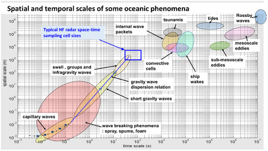
Figure 1.
Spatial and temporal scales of some oceanic phenomena. The effective resolution or sampling cell dimension when a skywave radar is used for remote sensing usually falls within the blue rectangle.
The vast coverage afforded by skywave propagation comes at the price of subjecting the radar signal to the prevailing structure and dynamics of the ionospheric plasma, which is host to a rich variety of phenomena, as shown schematically in Figure 2.
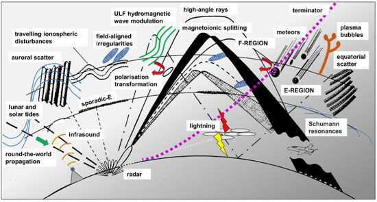
Figure 2.
Common ionospheric phenomena that impact HF radar.
Although we often look at this complexity from the perspective of the threat it poses to obtaining uncorrupted echoes from the ocean surface, and that is a very serious threat, we should not overlook the utility of any information that can be extracted about the ionospheric structure and dynamics, as this may be valuable to other user communities. Nevertheless, the primary societal benefits are undoubtedly those relating to the oceanic environment; skywave radar practice is very much about finding the most favourable windows of opportunity for conducting measurements.
For a number of practical reasons, we choose to separate the temporal variations of the medium into slow processes (structural change) and fast processes (dynamics) where the time scale defining the partition is loosely defined as the duration of the interval over which the range-rate of a discrete scatterer is linearly related to its observed Doppler shift. This definition allows for the presence of travelling ionospheric disturbances and other events that translate the Doppler shift but do not broaden it over the coherent signal acquisition interval.
With a few exceptions, it suffices to treat ionospheric radio wave propagation in the framework of ray theory, wherein the large-scale structure determines the ray trajectories and the resultant distribution of energy incident on the illuminated terrestrial surface. The strong diurnal variation of the structure effectively acts as a time-varying filter in range-frequency space, modulating the energy distribution, which must be monitored so as to guide the selection of radar frequency. Figure 3 shows several measurements of the echo intensity as a function of range (more accurately, group delay) and radar frequency, obtained with a backscatter sounder. The first (Figure 3a) sounder measurement was made at 1900 LT (local time), the second (Figure 3b) in the same direction but at a different time, 0100 LT, while the third (Figure 3c) was made at the same time as Figure 3a but in a different direction. The changes in distribution from day to day can be equally dramatic. This leads us to a fundamental constraint on skywave radar capability: a given region within the footprint of illumination can be interrogated by only a limited band of radar frequencies at any given time, so if a particular objective demands a specific frequency in order to deliver the desired measurement, it may not be available when it is needed.

Figure 3.
Examples of backscatter ionograms at different times of day and in different directions, illustrating the fundamental challenge of skywave radar: illuminating the area of interest with a suitable frequency. (a) Recorded at 1900 LT in direction 1; (b) recorded six hours later, at 0100 LT, in direction 1; (c) recorded at 1900 LT in direction 2.
In Figure 4, we provide an example of the relationship between the range bracket receiving adequate illumination for a particular mission and the band of radar frequencies able to provide it. This example also shows the echoes via multi-hop propagation; note that the range band of interest is illuminated by both one-hop and two-hop modes, offering two different frequency bands. The 2-hop mode has a longer group delay for the same ground range because it includes two ascents to the ionosphere. The ray geometry is illustrated in Figure 5.
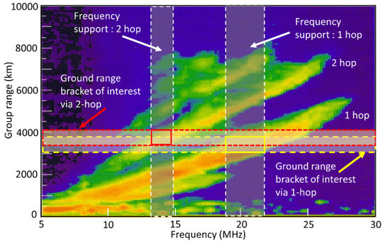
Figure 4.
A backscatter sounding showing the frequency support for the selected ground range bracket of interest. Both the 1-hop and 2-hop modes provide illumination, with available frequency bands [18.7–22.7] and [12.5–14.2] MHz, respectively. The 2-hop mode has a longer group delay for the same ground range because it includes two ascents to the ionosphere. The resulting windows of useful propagation are shown in the yellow and red boxes marked with solid lines.
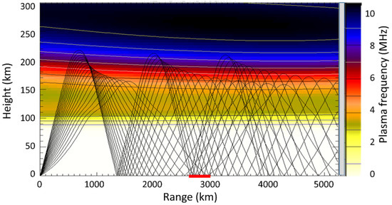
Figure 5.
Ray-tracing through a model ionosphere, showing the zone (marked in red on the abscissa) where 1-hop and 2-hop illumination overlap. At the frequency used here, no reflection from any lower layer—sporadic E appearing near 100 km altitude—occurs, nor does ducted propagation between the Es and F regions.
The detailed oceanographic (and other) information we might seek to extract from HF radar echoes is encoded in the Doppler spectrum. The structural or ‘quasi-static’ properties of the ionosphere, as we have defined them, do not degrade the form of the spectrum, so most of the oceanographic information is preserved. An exception is the estimation of ocean current information because the measured Doppler shift is biased by motions of the reflecting ionosphere. There are ways to overcome this problem, the simplest based on calibration using echoes from scatterers with known velocities, especially stationary terrestrial features such as islands.
The dynamic properties are a different matter altogether. Fluctuations of the electron density distribution in the ionosphere, arising from plasma wave processes, instabilities, tides, solar flares, and other phenomena, effectively cross-modulate the disturbances onto the transiting radio waves. If the spectrum of the modulation is very narrow-band, it can be removed by sophisticated signal processing at the radar receiver, but this is not always the case. A secondary effect of the plasma fluctuations is a modulation impressed on the polarisation state of the transiting radio wave, with implications for reception and echo interpretation. There are very few occasions when the effects of ionospheric dynamics are not a cause for concern when undertaking ambitious measurements.
Further complications arise from the simultaneous presence of multiple propagation paths to the same region for each hop, as illustrated in Figure 3, Figure 4 and Figure 5, because signals propagating via the different paths are usually differentially displaced in Doppler due to large-scale motions of the ionosphere and suffer different smearing effects. Figure 6 illustrates this situation with a range-Doppler map and the corresponding geographical reference map. Here, starting at 1150 km, the lowest range shown, we see echoes that propagated via the E-region on both outbound and return legs. Both land and sea echoes can be identified, with a small overlap due to the finite beamwidth. At a range near 1480 km, we see the earliest of the echoes that propagated via the E-region when outbound and the F-region when returning, and the converse. The clutter received via the mixed path is outlined with white dashes. There is a Doppler shift of 0.48 Hz at the earliest arrival, associated with the F-region reflection. Finally, at about 1550 km, we see echoes that employed the F-region on both outbound and return legs. These are outlined in magenta. As expected, the double passage via the F-region imposed a Doppler shift of 0.48 Hz on each leg, making 0.96 in total. The inset to the left of the range-Doppler map shows the Australian coastline over Darwin and parts of the Tiwi Islands encompassed by the radar beam. The correspondence between the land and sea clutter is unmistakable. Note also the raised ‘noise’ floor across all Doppler space over the Darwin city area (shown with a red ellipse). It isn’t noise, it is the composite of echoes from road traffic.
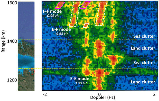
Figure 6.
A range-Doppler map showing the echoes from an interrogation region straddling the coast and extending beyond a nearby island. The distinction between land and sea echoes and the presence of multiple ionospheric propagation modes are indicated, as explained in the text.
An extension of the multi-hop mechanism is the possibility of trajectories involving sequential scattering from spatially separate zones on the Earth’s surface outside the nominal great circle locus, a phenomenon sometimes known as side-scatter and amenable to modelling [15,16]. This must be considered when observing extreme ranges. (A related form of indirect scattering occurs in the course of surface wave propagation, as first noted in [17] for a simple dipole source on the surface and generalised in [18], this has the effect of biasing oceanographic measurements made with HFSWR, so mitigating techniques [19] should be adopted.)
This menagerie of skywave complications motivated the adoption of a process model that made it straightforward to deal with the component propagation paths, in lieu of the conventional radar equation. The process model allows us to incorporate as much or as little of the prevailing physics as may be needed for a specific application under the prevailing circumstances, to optimise siting for particular missions, and to devise appropriate inversion procedures [20,21]. The received signal is represented as the output of a time-ordered sequence of operators acting on the selected waveform,
where
- represents the selected waveform;
- represents the transmitting complex, including amplifiers and antennas;
- represents propagation from the transmitter to the first scattering zone;
- represents all scattering processes in the j-th scattering zone;
- represents propagation from the j-th scattering zone to the (j + 1)-th zone;
- denotes the number of scattering zones that the signal visits on a specific route from
- the transmitter to the receiver;
- denotes the number of external noise sources or jammers;
- represents propagation from the i-th noise source to its first scattering zone;
- denotes the number of scattering zones that the l-th noise emission visits on a specific route from its source to the receiver;
- denote the maximum number of zones visited by signal and external noise,
- respectively;
- represents the receiving complex, including antennas and receivers;
- represents internal noise;represents the signal delivered to the processing stage.
This model can be generalised to handle moving transmitters and/or receivers by implementing the frame-hopping paradigm, using Lorenz transformation operators,
and
The possible relevance of this generalisation to the present study emerges when we consider hybrid radar configurations such as a ship-borne receiver piggy-backing on the transmissions from a shore-based skywave radar, though we shall not dwell on hybrid configurations here and instead refer the reader to [6].
Apart from the vagaries of the ionosphere, skywave radar must deal with external noise, which almost always exceeds internal noise. Of course, this is equally true of HFSWR but skywave radar antennas are typically designed to have maximum gain at elevations from which this external noise arrives, whereas HFSWR antennas can be tailored to reduce the response to signals arriving from non-zero elevation angles whilst preserving sensitivity to echoes arriving at grazing incidence. In any event, these additive components of the received signals must be dealt with by means of sophisticated signal processing that can suppress the unwanted noise without degrading the spectral purity of the desired echoes [22,23,24,25].
3. Skywave Radar Observables
3.1. The Role of Parametric Models of the Environment
The geophysical information that skywave radar delivers to users needs to be expressed in terms of familiar parameters in order to be assimilated with other data and exploited. It has been observed that the sea surfaces observed under many commonly-occurring conditions can be reasonably well represented by a rather modest number of parameters; the lexicons of operational oceanography and meteorology include widely-used quantities, such as significant wave height, dominant wave period and direction, directional wave spectrum, mean wind speed and direction at a 10 m height, convective instability index, rain rate, cyclogenesis potential, and so on. Accordingly, a radar’s remote sensing objective on any specific occasion may be phrased as the retrieval of a particular subset of these established parameters. As we have discussed in Section 2, the ionosphere is the final arbiter of the likely success of these retrievals, but for now, we shall set the space weather issues aside.
It has been largely taken for granted by the HF radar community that only a handful of meaningful parameters—observables—are accessible to this kind of sensor, with the most intimate description of the ocean surface being the directional wave spectrum and other parameters being extracted or derived therefrom. In order to see how this perspective short-changes prospective users, it is illuminating to reflect on the relationship between the radar observations, the physics used to model them, and the means of extracting the environmental information. To expand on this radar epistemology would take us too far from the immediate narrative; for now, we need only point out that, unless the physics describing a given phenomenon is taken into account in the model parameter space, it is hardly likely that the phenomenon will be identified correctly in the radar echoes. The inversion procedure that takes us from the space of echo data to a point in some multi-dimensional model parameter space will be effectively blind to the phenomenon, though the values retrieved for other, more conventional, parameters may well be misleading because an inappropriate model is being fitted to the data.
To illustrate, the best-known class of models corresponds to equilibrium states, where the directional wave spectrum takes a specific low-rank parametric form. In reality, there are realisations of the ocean surface that are not well represented by the equilibrium models. Wave field stationarity occurs for only a small fraction of the time in most locations, so retrieved directional wave spectra seldom lie close to the manifold of equilibrium states. However, even if we allow for non-adiabatic development of the sea surface geometry, we may have not freed ourselves from other assumptions built into the spectral representation of the surface. As an example, the standard model of the sea surface used in HF scattering theory (which we will review later in this section) is based on invariant form solutions of the linearised Navier-Stokes equation that are coupled by a weak nonlinear interaction term. Inversion of measured radar Doppler spectra to extract the directional wave spectrum is carried out by an operator parameterised by this coupling term. As it is known that the usual form of the coupling term is incomplete [26], estimates of the total directional wave spectrum and the nonlinear wave interaction contributions are inherently biased. It would certainly be incorrect to imply that the discrepancy is of great quantitative significance in most cases, but if interest focuses on the nonlinear mechanisms, then the retrieval will not be accurate.
Another important point to note is that some oceanic phenomena cannot be easily identified and quantified from the radar measurements of a single spatial resolution cell. For example, the development of waves with fetch and duration is revealed only by sustained observations over a large area. Similarly, the presence of oil spills, heavy rain, or ship wakes will perturb the wave spectrum, but this may not be recognizable from the inversion of echoes from the individual cell as the spectrum may lie close to the manifold of a free natural surface. Historical or adjacent contemporaneous data may be needed to reveal the anomaly, after which an expanded model parameter space can be constructed and used for subsequent inversion.
With all this kept in mind, we now review the scattering theory that lies at the heart of HF radar remote sensing of the ocean but generalised to accommodate skywave geometries.
3.2. Radio Wave Scattering from the Ocean Surface
The linearised scattering operator is properly represented by a polarisation scattering matrix, but almost all studies of HF sea scatter forgo the polarimetric formulation of the process model and reduce the scattering outcome to a power spectrum form for the dominant element. This is not unreasonable given that the typical resolution cell dimension usually exceeds the polarisation fringe spacing and that the incident polarisation state varies across the finite radar waveform bandwidth; further, the prescription of the sea surface geometry entering the scattering problem is customarily limited to second-order statistics. Nevertheless, it is always worthwhile keeping in mind where our theoretical developments have taken liberties and where a better model might deliver new capabilities.
The wavelengths of radio waves in the HF band are comparable with those of the most energetic surface gravity waves, and much greater than the surface wave amplitudes except in very high sea states. The intricacies of centimetre-scale capillary–gravity waves can be ignored from the electromagnetic standpoint (though not the hydrodynamic one) so the radar scattering problem can be formulated in the framework of small perturbation theory. As mentioned in the Introduction, the solution most widely used to model the power spectrum of the scattered field is that originally derived by Barrick [1]. An alternate form was developed by researchers at Memorial University, Canada [17] in order to replace the plane wave incident field treated in [1] by a different source, namely, a vertical dipole at the sea surface, but for skywave applications, the former is appropriate. For the skywave situation, the Barrick theory must be generalised to accommodate arbitrary elevation bistatic geometries and polarisations; such a solution was reported in [27].
In the following paragraphs, we review the principal results from this scattering theory, pointing out some features that are seldom mentioned explicitly because the usual context—remote sensing of an ocean surface subject to barotropic flow—does not require us to reflect upon the ‘obvious’ assumptions.
3.2.1. First-Order Theory
At the first order in the expansion, the expressions for the bistatic scattering coefficients obtained with the small perturbation method take the general form
where is the wavenumber of the illuminating radio wave, is a purely geometric function that takes different forms for skywave and surface wave radars, embodies the polarisation-dependence of the scattering amplitude, and is the spatial power spectral density of the surface evaluated at the Bragg-resonant wavevector given variously by
where is the unit normal to the surface, or
The scattering geometry is shown in Figure 7.
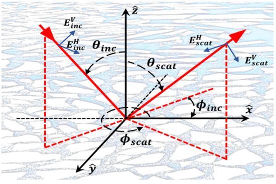
Figure 7.
The scattering geometry for bistatic skywave illumination.
Equation (1) can be viewed as the reduction of the integral form
where the delta function implements the Bragg condition.
The scattering coefficients defined by Equation (4) contain no explicit information about the ocean wave dynamics, as manifested in the temporal development of the radar echoes, most commonly expressed in the Doppler domain (although wavelet analysis and other time–frequency decompositions have their niche applications). For spaceborne microwave radars, the Doppler domain is seldom exploitable for remote sensing purposes, but for HF radars, Doppler information plays a central role in all geophysical investigations.
The extension of the scattering theory to time-dependent surfaces is accomplished by identifying the components that make up the spatial power spectrum with progressive waves whose spatial and temporal properties are linked by the dispersion relation that embodies the physics of the medium. In the case of small amplitude surface gravity waves on the free ocean surface, the relevant hydrodynamic equation is the linearised inviscid Euler equation, which leads to the familiar dispersion relation
Here, denotes the acceleration due to gravity and H is the water depth. For the case of first-order radar scatter, where only the free Bragg-resonant waves contribute, the observed frequency in a geocentric frame is given by
where the intrinsic wave frequency is augmented by the term , with denoting the local bulk motion of the water body due to any prevailing uniform (with depth) current.
Accordingly, the radar scattering coefficient for first-order scattering from the time-dependent surface takes the form
where now there is a dispersion relation constraint implemented by another delta function, supplementing the Bragg condition.
Numerous experiments have demonstrated that the selectivity of the Bragg scattering mechanism in HF radar observations of the sea surface is remarkable. Figure 8 shows one such example, recorded with a low power (15 W) HFSWR in Gulf St Vincent, Australia, in 1995.
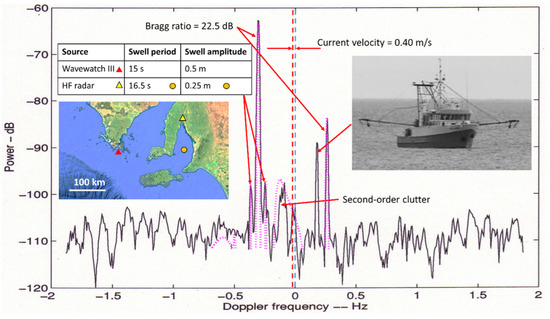
Figure 8.
The Doppler spectrum recorded from a resolution cell at a range of 150 km. The frequency offset due to the radial component V of an ocean current is indicated by the red vertical dashed line to the left of the black vertical dashed line at zero Doppler. The black solid line shows the radar measurement, while the dotted line is a theoretical model fitted to the data.
As in most instances, the spatial resonance is seen here as two peaks corresponding to , i.e., one from the waves approaching the radar and one for the waves receding, with positive and negative Doppler shifts, respectively. If the ambient current presents a non-zero component V aligned with ,
a displacement of the frequencies of the advancing and receding waves occurs, as indicated in the figure. For this measurement, a CIT of 100 s was employed, and it is apparent that the limit to the spectral width of the resonance peaks is set at least as much by the CIT and the radar waveform bandwidth as by the selectivity of the Bragg scattering mechanism. This selectivity is the key to the standard mission of measuring ocean currents, and accuracy is frequently cited as ±5–8 cm/s. Perhaps it is worth noting that assigning a single numerical value to current speed, or even to measurement accuracy, is, in a sense, misleading, as the surface current velocity, visualised as a point-wise defined quantity, will inevitably vary over a resolution cell in accordance with the turbulence commanded by the Navier–Stokes equation. Nevertheless, it maps directly onto the intuitive notion of bulk fluid motion.
Left unstated in this simple but widely adopted formulation is the assumption of barotropic current flow. Once baroclinic or shear flow effects appear, the non-zero vorticity renders the potential theory formulation of wave motions invalid, and a more sophisticated treatment of the fluid motions is required. The immediate requirement for many applications is the determination of the dispersion relation for surface gravity waves on defined shear flows, along with the associated inverse problem. Solutions for the dispersion relation on an arbitrary vertical shear profile were derived in [28,29,30] for the reduced (two-dimensional) case and used to obtain an expression for the effective mean current experienced by a wave of prescribed wavenumber , computed in the linear approximation. The general solution in this case takes the form
as the depth . This result has been used with various multi-frequency HFSWR systems to estimate current profiles [31,32,33,34], though the methods as reported rely on assumed parametric forms for the profile. More sophisticated models allow for Ekman stress and varying kinematic viscosity and extend the analysis to the second order; the HF radar signatures of these effects will be reported elsewhere [35].
Importantly, the phase velocity of a wave in the presence of shear flow is given to first order by
which states that there is no additional dispersion factor at this level of approximation.
Thus, from the HF radar perspective, it follows that there is no additional diagnostic value in the multi-frequency observations other than the access to varying depths over which the mean current is defined. Of course, if there is an extremely high Doppler resolution, high dynamic range measurements are available, and the use of a higher-order model would, in principle, provide access to independent information that could eliminate the need for any parametric model to assign a depth to a Doppler observation.
To illustrate the magnitudes of the shear-induced changes to the surface wave attributes, Figure 9 plots the phase speeds of co- and counter-propagating waves on a shear flow, where a surface current decreases to zero over a depth d. Here we have removed the surface current velocity component to focus on the intrinsic wave properties.
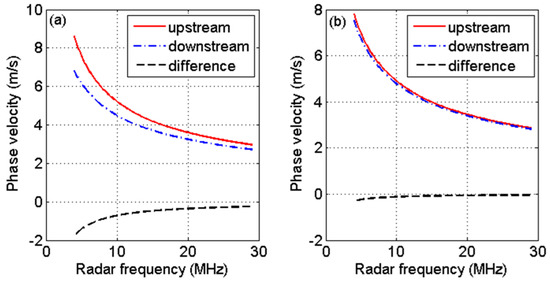
Figure 9.
Intrinsic phase speeds of surface gravity waves propagating on a shear flow. (a) High shear, U = 1.5 ms−1, d = 5 m; (b) Low shear, U = 0.5 ms−1, d = 10 m. In both cases the depth H = 200 m. The difference is plotted in the sense of downstream–upstream. The abscissa would normally be calibrated in wavenumber but, for convenience, we have converted this to the equivalent HF radar frequency corresponding to first-order Bragg resonance for backscatter geometry.
High-resolution measurements of near-surface current profiles in the open ocean are scarce, so the frequency of occurrence of the selected values used for illustration is unknown. What is evident is that the shear affects the Bragg line spacing and, hence, should be accounted for in HF radar observations.
A different but equally relevant phenomenon is the Stokes drift [36,37,38,39], resulting from low-order nonlinear effects. Regarding the first order, the contribution to the surface transport by the Stokes drift is given by
This can easily approach the magnitude of the wind-driven surface currents and is of obvious importance in the transport of surface flotsam, oil spills, and other surfactants. The question of whether HF radar actually measures the Stokes drift has entertained a number of researchers [40,41,42,43] but the answer is unequivocally ‘yes’.
Closely related to this effect is the interaction of surface winds with the top few millimetres of the ocean surface, resulting in wind drift [44] and wind-driven currents. Moreover, all of these phenomena need to be considered in the context of a rotating Earth and the associated Coriolis force that results in Ekman transport. While it is true that many of the observables targeted by HF radar can be described and retrieved without taking Ekman transport into account, the question needs to be posed and answered before proceeding with remote sensing schemes. Moreover, to conclude this digression, oceanic turbulence, mixed layers, and profiles of kinematic viscosity are further complications that exist, whether we recognise them or not.
Before progressing to review second-order scattering processes, it is worthwhile to stress yet again the signal corruption arising from ionospheric processes, which inevitably degrade Doppler measurement. Careful propagation management, coupled with adaptive signal processing schemes, maximises the availability of radar products, but high precision measurements of subtle effects such as current shear require very stable propagation conditions and, hence, are not routinely available.
3.2.2. Second-Order Theory
As valuable as the first-order scattering echoes are, they yield information extracted from only two waves of the continuum of waves present on the sea surface. That suffices to estimate the primary current parameters, along with crude information on the prevailing direction of the wave field and the surface winds responsible for their generation, but not much else. The hierarchy of multiple Bragg scattering processes also returns echoes that are observable when the radar has sufficient sensitivity, and these echoes yield information about all the waves on the surface. In the simplest interpretation of these processes, Bragg scattering from one wave train directs the incident radio wave not towards the radar receiver but onto a second wave train where another Bragg scattering event occurs. For every instance where the combination of the two Bragg scattering events has the resultant effect of directing the double-bounce scattered field towards the radar receiver, energy will appear in the Doppler spectrum, at a Doppler frequency given by the sum of the intrinsic frequencies of the two participating surface gravity waves,
while the sum of the wavevectors of the two participating surface gravity waves must satisfy
Having extended the electromagnetics model to the second order, we must do the same for the hydrodynamics. At the second order, a propagating disturbance associated with a wavevector can be expressed as an integral over pairs of first-order waves. In this case, the Bragg condition requires that
with as above, while the dispersion relation constraint requires that
with a physics-dependent coupling coefficient. However, a problem arises with waves on the free ocean surface as the dispersion relation (5) does not support free waves satisfying both (14) and (15). Instead, the resultant disturbance must exist as an evanescent wave, unable to propagate independently but phase-locked onto its parent waves, where it can still generate its own strong radar signature.
Combining the second-order effects, a Doppler continuum is generated, with its shape dependent on the amplitudes of all the gravity waves on the surface. The solution for the resultant second-order Doppler spectrum was developed in [1,27,45]; it takes the general form
where the kernel embraces both electromagnetic and hydrodynamic contributions. Expressions for as applicable to ice-free ocean surfaces take the form
where
with H as the water depth and the normalised surface impedance given by
Here, is the relative permittivity of seawater, σ its conductivity, the permittivity of free space, and the angular frequency of the radio wave.
These scattering formulae have been widely used in the context of monostatic HFSWR, where both the grazing angle and the bistatic angle equal zero, and to less extent in more general bistatic HFSWR calculations, but far less systematic study has addressed skywave radar configurations, perhaps on the assumption that there is not much new to find or exploit. The following examples are provided to counter that line of thought.
Figure 10 plots the sea clutter power spectral density as a function of Doppler and elevation angle, at fixed azimuth, for a monostatic skywave radar where the incident and scattered elevation angles are identical. We note the strong dependence on elevation and draw our attention to the subtle features on the shoulders of the spectra.
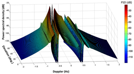
Figure 10.
Modelled clutter Doppler spectra for a specified sea state, varying only the elevation angle.
While informative, this figure is an incomplete description of the scattering signature observable with skywave radar. Polarisation transformation during propagation within the ionosphere means that the representation of the radar signal needs to include the polarisation state, from transmission through to reception, exactly as we have done in the process model formulation. Ideally, we should seek to construct the polarisation scattering matrix, but as mentioned earlier, the randomness of the sea surface leads us to settle for a power spectrum representation, so we use scattering coefficients defined by
where is the corresponding element of the scattering matrix .
Accordingly, the representation employed in Figure 10 needs to be expanded to that shown in Figure 11, where we used a slightly different format.
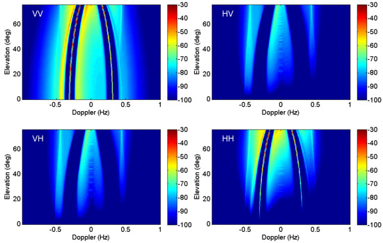
Figure 11.
Magnitudes of the elements of the power scattering matrix for similar parameters to those used in Figure 10. Colour bars measure power spectral density in dB/Hz.
This figure shows several important and under-appreciated features. First, the well-known result that the scattering coefficient for HH polarisation is far smaller than that for VV polarisation holds true at very low grazing angles but becomes of comparable magnitude for achievable skywave illumination geometries. A helpful way to show this is to plot the ratio, as presented in Figure 12.
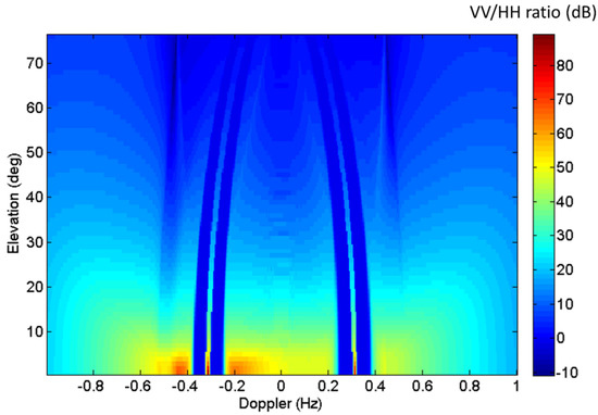
Figure 12.
The ratio of the VV power spectral density to that for HH polarisation, for representative sea conditions. The dark blue bands around the Bragg frequency are set to zero because both VV and HH polarisations have nulls there.
Second, the first-order components—the Bragg lines—vanish for cross polarisations, but not the second-order terms. Third, the co-polarised components are generally higher than the cross-polarised ones, but for parts of the Doppler spectrum and some sea states, the cross-polarised terms can exceed the HH terms. This has implications for HF beacon design.
Figure 13 shows the scattering signatures for the same sea state and incident illumination but bistatic reception with a bistatic angle of 60°. As expected, the Bragg scatter terms for cross-polarised elements are now present.
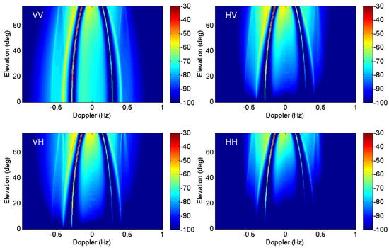
Figure 13.
Magnitudes of the elements of the power scattering matrix for similar parameters to those used in Figure 10, except that now the scattering geometry is bistatic, with an azimuthal separation of 60°. The Bragg lines no longer vanish for the cross-polarised elements. As before, colour bars measure power spectral density in dB/Hz.
While it is important to understand the dependence of the Doppler spectra on the scattering geometry, it is often sufficient, and sometimes easier, to understand from a visual presentation how the spectrum form changes with elevation. To this end, we subtract the spectrum at zero elevation from the other spectra and plot this difference. Figure 14 is a tableau showing the elevation-Doppler spectra (VV element) in the left column and the difference spectra on the right. The five rows correspond to radar frequencies of 5, 10, 15, 20, and 25 MHz. One avenue for exploiting this property opens when both single-hop and two-hop modes illuminate the target area.
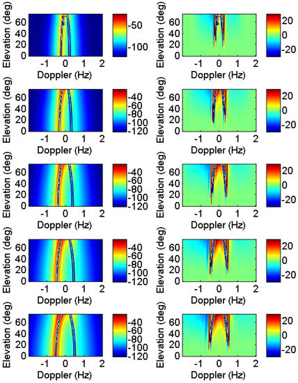
Figure 14.
Doppler spectra as a function of elevation at radar frequencies 5, 10. 15, 20, and 25 MHz (left column), and the same spectra after subtracting (in dB) the grazing incidence spectrum (right column). All colour bars on the left panels measure power spectral density in dB/Hz, while those on the right panels measure dB since they describe ratios.
Obviously, many parameters can vary in the modelling of this type, but the main effects are evident in the examples above.
In Section 3.2 we mentioned the common assumption that the full polarimetric treatment is unnecessary because individual radar resolution cells usually sample a mixture of incident polarisation states, so the spectral form of the dominant one (VV) can be assumed, with a small loss factor to account for the variation across the cell. While this is very often the case, it is not always true, and indeed, astute radar management can sometimes provide a degree of polarisation control. As evidence of this, we present in Figure 15 a range-Doppler map recorded with a skywave radar, and with it, theoretical modelling of the polarisation state ‘thumbprint’ for the corresponding geography and time, as computed using a modified IRI ionospheric model.
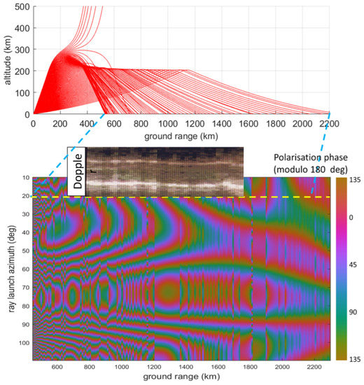
Figure 15.
The main figure shows the polarisation map predicted for a particular radar, frequency, and ionospheric environment, with the polarisation phase (angle of the principal axis of the electric field) shown in colour using a cyclic colour scale. Experimental data showing a quasi-periodic intensity modulation of the sea clutter, presented in grey-scale, is overlaid at the single azimuth at which it was measured; the modelled ray fan for that azimuth is plotted at the top [46]. The peaks in clutter intensity align with occurrences of the vertically-polarised incident field.
The polarisation-induced modulation of the clutter echo power is in reasonable agreement with the model; we do not have access to the raw data so as to compare the spectra, but the prospect is enticing and there is reason to believe that polarimetric skywave radar is under consideration [47].
3.3. Remote Sensing of the Ocean Surface with HF Radar
The basis for almost all present-day HF radar remote sensing of the ocean is the notion that candidate geophysical phenomena above, on, and under the air-sea boundary modify the time-varying geometry of the interface and thereby write their signatures into the radio wave field scattered from the surface. One can imagine other manifestations of the ocean dynamics, such as geomagnetic, acoustic, or gravitational perturbations that imprint on the ionosphere and modulate transiting HF radio waves, but these effects are, in almost all cases, too weak, too cryptic, or too obscured by other ionospheric motions to be discerned. One important exception is the detection of tsunamis: the Rayleigh waves generated by seismic events couple to infrasonic waves in the atmosphere; these waves propagate to the ionosphere where their signature is evident to HF radar [48,49,50,51].
Here, we need to be very specific: the signature of a phenomenon is the difference between the radar output when the phenomenon is present and the output when it is absent, all else remaining the same. Clearly, it depends on the radar system characteristics and the measurement procedure, pointing to the oft-ignored fact that matching the measurement procedure and choice of selectable system parameters to the characteristics of the target observable is the key to successful measurements.
The atmosphere–ocean system is host to many distinct phenomena, most of them tightly coupled or linked to others. We have attempted to indicate this complex in Figure 16, though even this presentation is incomplete. The captions shown in red indicate phenomena for which HF radar signature theories have been developed, though we hasten to add that not all of these have been observed experimentally. Those printed in purple are of interest for their indirect effects on HF radar scattering; experiments directed at clarifying the relevant properties have been performed using microwave radars within the HF radar research programs.
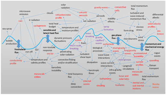
Figure 16.
Some of the principal oceanic and atmospheric phenomena that have been considered by the HF radar remote sensing community. Specific signature models have been developed by those shown in red.
The conventional approach to HF radar sea echo analysis proceeds in the temporal power spectrum domain where Doppler frequency shifts are manifested, along with other phase modulation processes, though the spectrum itself is phase-blind. In its most direct implementation, the retrieval of sea surface parameters from the sea clutter echoes is achieved by inversion of the equation that sets the measured Doppler spectrum to be equal to the sum of the first and second-order contributions as given by Equations (10) and (19), filtered by the overall system transfer function to account for radar system parameters, propagation considerations, and signal processing algorithms.
In this idealised model, the most informative retrievable quantity is the directional wave spectrum , from which other properties can be computed or inferred through mathematical models that incorporate the relevant physics. At the simplest level, the omnidirectional (non-directional) spectrum and the significant wave height are obtained by direct integration,
projecting the directional spectrum onto the nondirectional spectrum and thence to the significant wave height, where is the surface displacement and the kernel embodies the appropriate Jacobian where required. Similarly, dominant wave period and direction, and swell parameters, can be inferred from the directional wave spectrum, as has been widely reported in the literature.
A seemingly fundamental limitation arises with single radar observations, namely, the left-right ambiguity about the radar observation axis. Various methods have been developed to overcome or at least mitigate the associated echo interpretation uncertainties. These include (i) the exploitation of wave spectrum development models that account for fetch and duration, (ii) second-order echo components dependent on the swell, for which directional estimates are usually available, (iii) any in situ measurements or ship reports that can be used as seed values to which continuity arguments can be applied, (iv) climatological values, (v) recognition of characteristic wind systems such as fronts and storms, (vi) island wakes, and (vii) bistatic and/or multi-frequency observations using auxiliary systems. Nevertheless, the ubiquitous non-stationarity of wave fields in space and time can, at times, frustrate even the most diligent attempts to remove the ambiguity altogether.
Techniques for estimating from trace back to 1977 [52,53,54], though these early techniques made unrealistic assumptions about the form of the spectrum; subsequent methods evolved in a number of directions [55,56,57,58], and now there is an extensive literature on the subject, though much more remains to be done. Essentially, these methods fall into four categories: (i) linearisation of the integral equation by mathematical approximation, (ii) linearisation of the integral equation by physical assumption, (iii) formulation as an optimisation problem in some parameter space associated with common wave spectrum models, and (iv) empirical mapping by syntactic or statistical pattern recognition techniques.
It would be challenging enough that these approaches all confront the intrinsic difficulties of inverse problems, and most need auxiliary stabilizing measures such as Tikhonov regularisation or singular value decomposition, but there is in addition a more basic problem. Often the quality of Doppler spectra recorded via skywave propagation is compromised to the extent that extraction of the directional wave spectrum is not achievable. To accommodate this circumstance, many empirical techniques have been developed to obtain estimates of less detailed descriptions or individual parameters from robust features in the Doppler spectrum (see e.g., [59,60,61,62]). By robust, we mean ones that largely survive the signal degradation incurred during propagation or resulting from radar system deficiencies and external radio interference. The Bragg line ratio is the prime exemplar, but there are others. Not surprisingly, many of these parameter estimation techniques were developed in the context of HFSWR, where the same or analogous corrupting factors prevail, but one entire stage of retrieval methodology is almost unique to skywave radar. We refer to techniques for sophisticated pre-processing of the radar echoes to remove or at least ameliorate the contamination and signal distortion caused during propagation. This topic will be dealt with in Section 3.4.
Yet another complication must be acknowledged. Although the operational practice of HF radar remote sensing is overwhelmingly based on the notion of the directional wave spectrum as a faithful representation of the physical system it describes, there is a contradiction at its heart arising from the essential nonlinearity of ocean surface hydrodynamics. In order to retain the simplicity, elegance, and practical utility of the wave spectrum model, formally a linear construct, it must be modified to allow for weak interaction between its elements. This was recognised at the outset [1,63,64], and a term incorporated in the Barrick expressions for the scattering coefficient, as noted in Section 3.2.2. While the resulting approximation to physical reality is far superior to one based on a purely linear spectrum model, it is still an approximation, so various ways have been explored to improve the fidelity of the description without sacrificing its convenience and ease of engineering application [21,65,66]. We shall not pursue these here but make the following point: some oceanic phenomena of interest present signatures that reflect the strong (even dominant) role of hydrodynamic nonlinearity. In these cases, the fidelity of the treatment of nonlinearity in the scattering theory is of critical importance [20,67]. Then there is the issue of how the hydrodynamic nonlinearity manifests itself in the electromagnetic domain, i.e., the radar echoes. The limitations of standard second-order statistics in this context have long been recognised, leading to exploratory studies of the use of higher-order statistics and their polyspectra [68,69], but the issue remains unresolved.
HF sea clutter inversion procedures are almost invariably formulated as mathematical operations acting on a single realisation of a Doppler spectrum. Superior approaches to the estimation of some phenomena, including many shown in Figure 16 and some listed in Table 1, proceed by exploiting physical models that connect a given phenomenon of concern to its impact on the set of directional wave spectra observed over an extended region of the surface and sampled over an interval of time, rather than a single Doppler spectrum recorded from an individual resolution cell. It follows that the input data samples a process that is inhomogeneous and nonstationary, and, hence, involves the mechanisms of wave generation, nonlinear interaction, and dissipation, acting together to govern the development of wave fields in space and time, and modelled by the Action Balance Equation (see e.g., [70]).

Table 1.
Prospective observables and their signature mechanisms.
Rather than review these methods, established or emerging, we shall illustrate the kinds of skywave radar products that have a long history of successful implementation and delivery to clients. These will provide the basis for assessing the societal utility of our technology, though we emphasise that the examples given do not exhaust the range of possibilities.
Figure 17 shows a Jindalee radar map of the dominant wave period recorded in 1985, covering the Sulu Sea between Malaysia and the Philippines, i.e., a range bracket from 3500 to 4000 km. On this occasion, the dominant waves had periods ranging from roughly 2–5 s, with the median in the central area perhaps 4 s, corresponding to a wind speed of 6 m/s, i.e., 12 knots. This range was in agreement with climatological wind speeds for the Sulu Sea. Close inspection of the figure also reveals a consistent displacement of the echoes from land, shown in white, from the geographical map overlay, as if the radar footprint had been rotated from the true steer direction during plotting. In fact, the cause was a tilt in the ionosphere, a nice example of the coordinate registration problem encountered with skywave radar and addressed by this technique since 1983 [13].
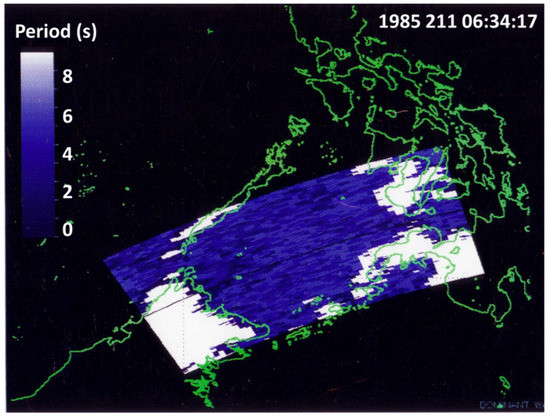
Figure 17.
A skywave radar map of the dominant wave period in the Sulu Sea. Note the displacement of the land echoes (shown in white) from the map outline; this is a result of tilts in the ionosphere.
To illustrate the synoptic scale mapping of significant wave height, Figure 18 shows a Jindalee radar map of this parameter around Tropical Cyclone Victor, measured in March 1986. The fidelity of the method used for this retrieval is borne out by the characteristic spiral band signatures, with exactly the wave height asymmetry predicted for the known direction of travel of the cyclonic system. Based on radar observations of several such events, a parametric model of the wind and wave fields around tropical cyclones has been developed [71].
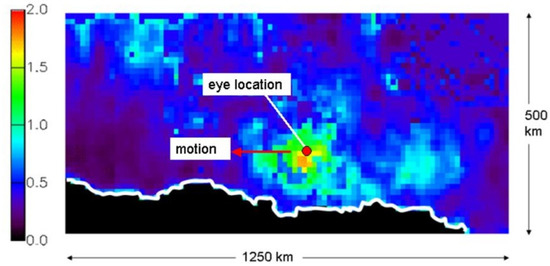
Figure 18.
A skywave radar map of the wave height around a tropical cyclone, TC Victor, in 1986. The spiral band structure is very clear.
The mechanisms that couple the water body bounded by the sea surface to the motions of the air immediately above it result in fluxes of momentum, mechanical energy, sensible and latent heat, gas species, and fresh water. In particular, the surface wind is ultimately responsible for exciting the ambient ocean wave field, so, in principle, a sufficiently well-behaved physical model relating the wind stress to features of the wave field can be inverted to retrieve the wind direction and speed from the measured radar Doppler spectra. This is exactly the approach taken in [2,3] and by many others since (e.g., [5,72,73,74,75,76,77]), using simple expressions that assume a single-valued function mapping wind direction to the ratio of the first-order Bragg peak intensities. A more sophisticated methodology places less reliance on models such as that used in [2,3] or the spreading function, but even these simple models yield reasonable results most of the time. Figure 19 presents an example of the kind of synoptic wind direction data that can be extracted. In this example, recorded with the Jindalee Stage B radar in 1984, the radar took less than 5 min to complete the entire mapping exercise. There is one important though not critical caveat: no attempt has been made here to assign the left-right ambiguity associated with single radar observations. An early example of a map in which the ambiguity has been resolved is included here as Figure 20; this is the wind direction map corresponding to the significant wave height map shown earlier in Figure 18.
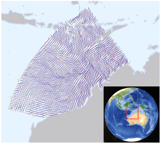
Figure 19.
A map of wind direction covering over 2 million square kilometres, plotted at a degraded measurement resolution of ~25 km.
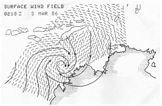
Figure 20.
A low-resolution map of the wind direction recorded from Tropical Cyclone Victor in March 1986 [76].
The estimation of wind speed has been attempted by a variety of empirical methods, most of which rely on assumptions that are difficult to justify except in special cases. The difficulty arises from the fact that wave development occurs over significant intervals of space and time, so an accurate measurement of the directional wave spectrum cannot be associated with an equally accurate estimate of the ambient wind field by means of a simple parametric relationship. However, studies of the HF radar signatures of wave fields evolving under the action of time-varying winds show a consistent pattern of development that offers a valuable diagnostic capability [78].
Somewhat surprisingly, ocean current measurement, the staple of HFSWR, is often possible with skywave radar. As with the former, it is the first-order echo from the -aligned component of the surface current vector that is used to estimate a component of the surface current vector, though ionospheric motions frequently preclude the accurate estimation of current velocity from a single observation except when zero-Doppler references are available, as with islands and offshore oil rigs [79]. However, even when no such ground-truth reference is available, the fact that currents vary on a timescale of days or longer means that multiple radar measurements can be acquired. It is then possible to exploit knowledge about the large-scale spatial and temporal properties of travelling ionospheric disturbances and their effects on radio wave propagation to obtain reasonable estimates [80].
With two skywave radars illuminating the same region, full current vectors can be extracted, as with most HFSWR deployments. An example of this was reported in a series of experiments using two US Navy ROTHR radars to study flows in the Caribbean and the adjacent Atlantic Ocean [81,82].
Beyond what we might call routine observables, those illustrated above, a number of fascinating extensions to the standard wave spectrum monitoring mission have been explored over the past several decades. The common thread to these investigations is the recognition that localised changes in the wave field structure and dynamics may arise from very specific meteorological, oceanographic, hydrological, cryological, or human activity-induced phenomena. We need to be cautious when discussing these prospective capabilities as they have not all been demonstrated operationally, or a particular phenomenon may require especially clement conditions in order to yield a discernible signature, but physics tells us that the reaction of the ocean surface geometry and dynamics to the presence of these phenomena can be substantial. Over the years, the associated HF radar signatures have been modelled in considerable detail and armed with these models, some of the phenomena have been identified in recorded data. A short list of what we shall call prospective observables is given in Table 1, along with the mechanisms generating the signatures and references.
3.4. Dealing with Imperfect Data
Conventional analysis sets as its ultimate goal the estimation of the directional wave spectrum in each range-azimuth cell, but, as we have seen, this objective is often frustrated by confusing ionospheric structure and ionospheric dynamics-induced signal corruption, as described in Section 2, and by inadequate CNR (clutter-to-noise ratio) due to the prevailing ionospheric structure and/or high levels of external noise. With reference to the process model, we observe the echo after our radiated waveform has been subjected to though, for oceanographic remote sensing purposes, we are interested only in how modifies the incident waveform, thereby writing the ocean’s signature on our signal.
Rather than simply extract whatever information has survived the signal corruption, it makes sense to apply signal processing techniques designed to remove much of the distortion and contamination experienced by the radar echoes. As the radar must deal with the signal after it has been subjected to both outbound and inbound propagation paths, it is necessary to assume commutativity of the process operators, i.e., , and then seek an approximate inverse to the operator , which can then be applied to the received signal in the appropriate domain, certainly including the time dimension and possibly others. The successful construction of relies heavily on the incorporation of realistic physics; in this regard, the pioneering work of [94,95,96] set an example that has been followed by many others.
Sometimes this approach can be extremely effective, especially when the consequences of the joint operation of multiple corrupting mechanisms are taken properly into account [97], though all too often the propagation effects are beyond redemption. As an illustration, Figure 21 shows the progressive clean-up of a measured Doppler spectrum as successive signal processing algorithms are applied.
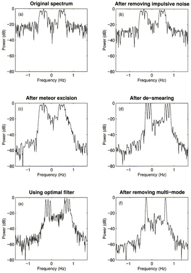
Figure 21.
Progressive clean-up of skywave radar sea clutter that has experienced the most common forms of contamination and distortion. The progressive signal processing measures are indicated in the titles of the individual panels (a–f).
What is not visible in this kind of demonstration is the need to solve a precursor problem: before we apply some ambitious repair algorithm to the echo data, we need to diagnose the kind of distortion that is present, and only then apply the appropriate corrective measures. The blind application of inappropriate measures can easily do more harm than good. An important step in distortion diagnosis was the development of a test to discriminate between multimode broadening and phase smearing distortion, two common and quite different mechanisms that could yield the same resultant Doppler spectrum, though the treatment algorithms needed are totally different. Again, referring to the process model, for the simplest case of discrete multimode on any skywave path, is given by (with various caveats that we will ignore in this illustrative example)
where the summation is shown for two modes present, E-region and F-region, say, with amplitudes and constant (for the duration of the coherent integration) Doppler shift . A double pass process—a radar observation—then involves four paths in total, two of which might seem equivalent but are in fact differentiated by various subtleties and antenna patterns. If multimode is indeed the affliction on some occasions, it was shown in [98] that the asymmetry in a typical sea clutter Doppler spectrum results in different subdomains of useful information depending on the direction of the differential Doppler shift between modes. The more ambitious goal of deconvolving the multimode is complicated by the spatial separation of the cells on the ocean sampled by the different mode combinations but arriving at the same group delay. A second problem is the elevation angle dependence of the clutter spectrum as treated in Section 3.2.
Operationally, a fully automated system is highly desirable, but the diversity of spectral forms poses a challenge to the development of computer-based quality and retrieval algorithms. A rudimentary implementation of a quasi-operational scheme was reported in [98,99], where Doppler spectra were sorted into 9 categories according to suitability for detailed analysis (SDA), with 9 indicating the highest quality. From the user’s perspective, coverage extent can be almost as important as the detail of oceanic information, so studies were undertaken to assess availability. Modern radars have far superior performance to those of forty years ago but some statistics from that era are still useful, not least because they indicate diurnal variation. Figure 22 presents histograms of availability against effective range depth, plotted for different periods of the day, corresponding to morning, afternoon, and evening. As expected, top-quality propagation is less frequently available, but at almost all times, the instantaneous range depth exceeds 500 km and often 1000 km.
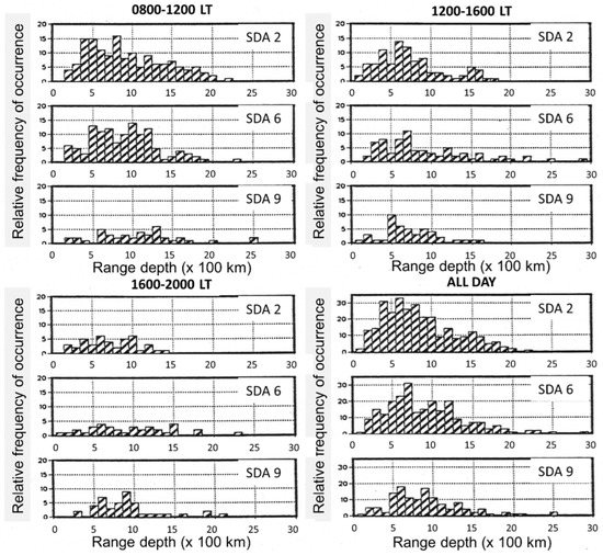
Figure 22.
Distributions of data quality against instantaneous range depth for different periods of the day.
What is equally encouraging is the observation (based on many years of experience) that even range-Doppler maps that appear irretrievably corrupted by complex propagation structures and dynamics can still yield useful information when sophisticated signal processing is employed. Figure 23 presents one example of a high-quality range-Doppler map together with five examples showing increasingly dramatic departures from the ideal. In each case, data from five adjacent beams are presented, each with twenty range bins. These examples spanned range brackets of typically 500 km depth, located at various positions between 1500 and 2500 km from the radar, and all were recorded in the daytime. In every case, some useful information was retrieved.
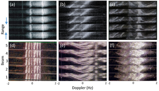
Figure 23.
Azimuth-range-Doppler maps for different propagation conditions, showing the variety that signal processing must deal with. (a) ideal propagation, (b) range-dependent Doppler shift, (c) multiple modes with range-dependent Doppler and leading-edge effects, (d) E-E, E-F and F-F modes with mode-dependent Doppler shift, (e) leading edge of F-mode seen via E-F and F-F, with magnetoionic splitting and traces of E-E mode, (f) diffuse multimode with travelling ionospheric disturbance.
As a final example of the kind of data that can yield to the analysis, Figure 24 shows a range-Doppler map with a clear land-sea boundary roughly halfway through the range bracket, along with echoes from a cluster of small islands. There is obvious broadening in Doppler, along with possible unresolved multimode and a range-dependent Doppler shift. The echoes are strong from beams 5–10 but become progressively weaker in the lower beams. Rather poor quality, it might seem, but this coastline lies at a range of over 8000 km. Together, the coastline and island echoes enabled geographic registration in both range and azimuth to within 20 km; without them, the position error exceeded 200 km in both dimensions. Moreover, the broadened first-order echoes easily support the estimation of the Bragg ratio, even without sophisticated signal processing—the figure plots raw Doppler spectra with no remedial steps, as used in Figure 21.
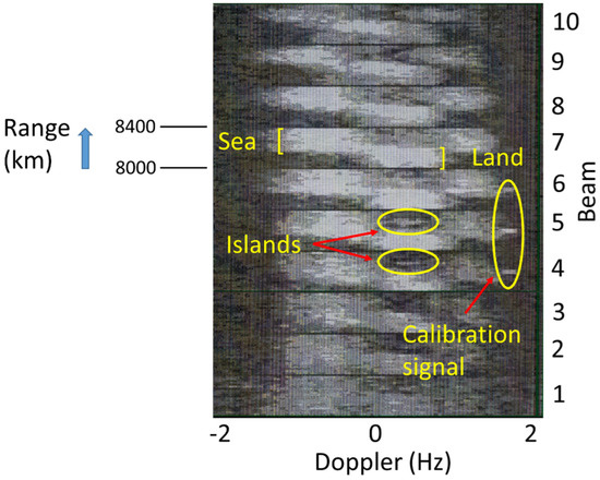
Figure 24.
A nested range-azimuth-Doppler map recorded from a footprint at a range exceeding 8000 km; the various echo sources are indicated. Each beam has the same range extent, but it is marked only on Beam 7.
Once again, we stress that such extreme performance is not always achievable. Moreover, any windows of opportunity may be short-lived, perhaps half an hour, so an important part of radar management is finding these windows when they occur and adapting the task list accordingly. A source that provides this kind of synoptic, persistent overview of conditions is an essential part of an HF skywave radar system [100].
Much of the discussion in this section has been aimed at convincing the reader that remote sensing of ocean conditions with skywave radar is fraught with challenges that do not have direct counterparts in HFSWR, but the combination of astute frequency management and powerful signal processing techniques are effective tools in achieving a worthwhile radar capability. This assertion was examined and acted upon by program managers in (at least) two major HF radar program offices in the past, each of which then undertook an evaluation of the potential economic benefits that would come from the deployment of skywave radars for societal applications. In each case, the assessment was based not just on modelling but on extensive exposure to operational HF radars and, in one case, to a large body of remotely-sensed wind field maps. We review these studies in the following section before examining the present-day situation, where both technology and applications have evolved dramatically.
4. Assessment of Societal Utility
4.1. Historical Assessments
In 1974, the Environmental Research Laboratories of the US National Oceanic and Atmospheric Administration (NOAA) issued a substantial report titled ‘Economic Appraisal of Real-Time Synoptic Sea-State Measurements by Over-the-Horizon Radar’ [101], which set out to quantify the prospective benefits of deploying skywave radars for societal applications. The report consists of four sections: (i) Why measure sea state? (ii) Real-time sea state measurements by over-the-horizon radar, (iii) alternative sea state measuring techniques, and (iv) economic analysis of over-the-horizon sea state radar. NOAA already had considerable experience with HFSWR, especially through the support of Don Barrick, indisputably the leading authority on the subject, but rather less detailed familiarity with skywave radar.
The first section of the report identified the following users of sea state data: commercial shipping, ocean fisheries, naval operations, off-shore oil operations, marine science, off-shore mining, search and rescue, shoreline damage and erosion, and recreation, and noted that existing sources of such data were ‘inaccurate and untimely enough that only moderate use can be made of them for such purposes as optimum ship routing’. A table (reproduced below as Table 2) summarised the various industry expenditures and the most needed sea state requirements.
Table 2.
Summary of sea state users and needs (from [101]).
The second section reviewed the basics of HF scattering from the ocean surface, then described the subsystems that make up an OTH radar, the performance characteristics, the costs involved in building such a radar designed for sea state measurements, and the issue of siting. While the scattering theory has not changed, much of the other material is no longer valid, but the discussion of siting is still relevant today. In particular, the proposed sites and coverage for networks covering shipping routes across the Pacific and Atlantic Oceans are not only meaningful but actually reminiscent of some of the major OTHR systems deployed more than a decade later by the USAF and USN. We reproduce these maps in Figure 25 and Figure 26 because of their ongoing relevance.
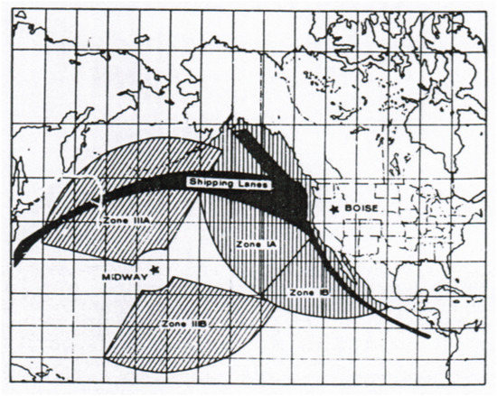
Figure 25.
Proposed sites and nominal coverage for Pacific radars envisaged by Rhodes and Chadwick [101].
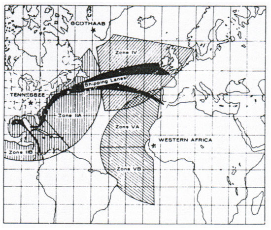
Figure 26.
Proposed sites and nominal coverage for Atlantic radars envisaged by Rhodes and Chadwick [101].
The third section of the NOAA report dealt with the alternative technologies—data buoys, satellite observations, and ship reports. In 1974, satellite-based remote sensing was in its infancy, so the assessment of radar altimeters (GEOS-C) and synthetic aperture radar (SEASAT-A, to be launched in 1977) is no longer meaningful, though it remains true that the detailed wave spectrum information that can be obtained with skywave radar is far more detailed than any spaceborne sensor can achieve. Finally, the NOAA report looked at the construction and running costs for the candidate radars shown in Figure 25 and Figure 26 and compared these with estimates of the economic benefits for the various user communities. The relevant table from the report is reproduced here as Table 3.
Table 3.
Benefit and cost summary ($M).
The numbers cited are, of course, meaningless today in absolute terms; indeed, as one who was designing skywave radars in the 1970s, the present author is of the view that some of the estimates (e.g., operating costs) were highly optimistic even in 1974. Nevertheless, the report remains the most thorough assessment of the economics of the broader societal benefits latent in skywave radar and is a testament to the far-sightedness of NOAA.
A far less ambitious study was undertaken in Australia in 1983. Once the remote sensing capabilities of the Jindalee Stage B skywave radar had been firmly established [102], the commercialisation office within the host organisation (the Australian Defence Science and Technology Organisation) surveyed the potential user community, to estimate the economic value of the radar’s remote sensing products. Prospective client groups included commercial shipping companies, offshore oil and gas producers, and the national weather forecasting agency. Under what seemed to be plausible assumptions, a rough estimate of the potential economic value of the radar ocean sensing products was obtained. The nominal sum remains confidential, but we can state that it far exceeds the actual running costs of the radar. Subsequently, several of the remote sensing techniques were patented but the idea of commercializing the remote sensing output was abandoned, primarily because it became apparent that this mission would consume too much of the radar timeline, which was heavily focused on air and surface surveillance. In spite of this, the scientist designer of the ship detection functionality clandestinely inserted code that extracted remote sensing data whenever the Jindalee radar carried out its ocean surveillance mission, and this information was sent to the Australian Bureau of Meteorology for assimilation with other data sources. The Bureau acquired this data for a decade and reported on its value to their forecasting [103] before other factors intervened and the radar input ceased. A history of the early years of the Jindalee radar remote sensing activities has been published in [13]; it gives more details on this sequence of events.
4.2. Contemporary Assessment
In this section we present a brief modern assessment of the prospective societal benefits of skywave radar, starting with the nine categories chosen by Rhodes and Chadwick [101], then adding several more to accommodate applications that have emerged since 1974. In most cases, we have added considerably more technical detail and experimental results to support our assessment of the requirements of modern user communities. However, being acutely aware of our limitations, we do not attempt to assign economic costs and benefits, a task we leave to our readers from the respective communities.
We may start by examining Figure 27, where we have plotted the nominal coverage of the major skywave radars actually in operation at the time of writing, indicated by colour shaded areas superimposed on a map of global shipping routes. The former ECRS and WCRS, USAF skywave radars operating on the east and west coasts of the US from the late 1980s, but progressively dismantled between 2005 and 2010, provided excellent coverage of the entire North Atlantic Ocean and much of the North Pacific Ocean. For reference, we have added their nominal coverage with dashed lines, on the basis that the US appears to have renewed interest in this technology and most of the real estate is still available, so a rebirth is conceivable.
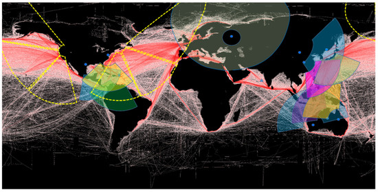
Figure 27.
Nominal coverage of some major HF radars presently in operation (shaded in various pastel colors to enable them to be identified), together with that of the former (and possibly future) ECRS and WCRS radars (shown by dashed yellow lines).
We have chosen not to discuss the HF radars of the SuperDARN network, a class of radars whose primary role is line-of-sight observations of the plasma turbulence in the high-latitude ionosphere [104,105]. There have been some very limited attempts to extract oceanographic information from the distant sea surface echoes when they are visible [106], but the design and operating modes of these radars yield very poor results.
We can see that the East Asian sector shipping routes are reasonably well covered, but many other heavily-traversed routes are not within the primary illumination zones of existing skywave radars. It is likely that, in several years, the situation will be rather different, with a number of radars reported to be in the design stage. In what follows we look at the candidate domains of societal application.
4.2.1. Shipping
At the time of the Rhodes–Chadwick report [101], there were some 21,000 ocean-going ships. Today, there are over 55,000 merchant ships and thousands of large fishing boats that cross the oceans. Figure 28 shows a coarse sampling snapshot of ships reporting via AIS, the Automatic Identification System operated by the International Maritime Organisation (IMO) [107]; this kind of picture can show only a small fraction of the actual number of vessels, but even so, it shows clearly that the oceans are busy spaces with much to interest surveillance and monitoring systems.
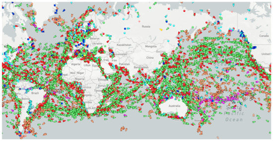
Figure 28.
A snapshot of merchant shipping vessel locations as reported via AIS. (Map courtesy of MarineTraffic, [107]). Colors indicate type of vessel, e.g., red for tankers, green for cargo ships, pink for fishing boats.
A key concern on the part of the owners is the efficiency of the chosen sailing routes. For a container ship, basic running costs are now typically USD 50,000 to USD 100,000 per day, exclusive of fuel, which, at today’s prices, may exceed USD 150,000 per day. Thus, any saving of more than a few hours on a voyage is well worth seeking.
Not surprisingly, there is a strong demand for expert guidance on optimum route selection. A side benefit of employing routing services is that vessel insurance premiums reduce over time as the incidence of unwelcome events decreases. The goal is to design the ‘best’ route, building on the available wind and sea state forecasts, together with knowledge of ocean currents that might be exploited, and then taking into account the ship characteristics, the cargo being conveyed, safety of the crew, any risk of damage to the vessel, and so on. Fuel usage varies with sea state, as does transit time, and there may be other considerations such as passenger comfort or the need to arrive at a specific time because of berth availability. (To be moored waiting for a berth can easily cost USD 150,000 per day.) Thus the metric used for optimisation varies according to circumstances.These companies rely on real-time meteorological and oceanographic data from national weather services, usually via the forum of the World Meteorological Organisation. For oceanographic conditions, the WMO collects and filters data from roughly 100 moored buoys (observatories) and 1000 drifting buoys, together with reports from cooperating ships and aircraft, along with data from some 30 meteorological and 200 research satellites [108]. The quality-checked products are made freely available to every country in the world through the WMO Information System (WIS). A map showing some of the moored buoys is presented in Figure 29; the ones shown are managed by the Data Buoy Cooperation Panel. A few companies supplement these data sources with their own buoys, but almost all effective ship routing is predicated on the availability of timely WIS data.
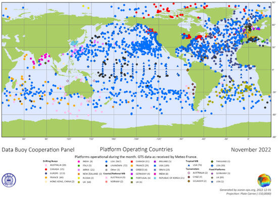
Figure 29.
Locations of fixed buoys operated through the Data Buoy Cooperation Panel.
This might seem like a lot of input of measurements from which to generate the desired information but when compared with the density of prospective skywave radar observations, on a 25 × 25 km grid, say, as illustrated in Figure 19, or even finer, the sparsity of detailed, instrumented surface observations is apparent. Moreover, we should add, not all these buoys report as scheduled, their instruments can lose calibration or fail, they need maintenance, and, hence, they share with skywave radar the property that they are not perfect. Further, the timeliness of the data being assimilated can ‘lag’ the pace of change in the sea conditions. Moreover, the buoys measure the environmental parameters at a single point, whereas the radar integrates over a resolution cell; in almost all circumstances, i.e., a more meaningful quantity to the seafarer. That said, we hasten to point out that moored buoys can enhance the skywave radar products by providing in situ validation of radar-derived estimates of ocean parameters at fixed locations.
Based on these sampling densities, it is obvious that skywave radar has a role to play in improving the quantity of remotely-sensed ocean data, as could be used for route optimisation. The radar can also extend the quality and detail of the wave information, by providing direct measurements of the directional wave spectrum, which lies beyond the capabilities of the buoy networks. Knowledge of is essential for many purposes. In particular, the amplitude, frequency, and direction of the swell are of vital concern to ships, especially when the wave frequency is close to one of the resonant frequencies of the ships’ six degrees of freedom. Even when there is no resonance, the distribution of load over the wave surface can be critical. This was strikingly demonstrated by the break-up of the post-Panamax container ship MOL Comfort off the coast of Yemen in June 2013 [109]. The stresses imposed by sagging and hogging—the hull slumping into troughs and folding over crests as pictured in Figure 30—exceeded the strength of the loaded hull and resulted in the vessel breaking in two. Ships need to change course when threatening conditions arise, but buoy observations of scalar wave height are of no help; the directional information is vital.
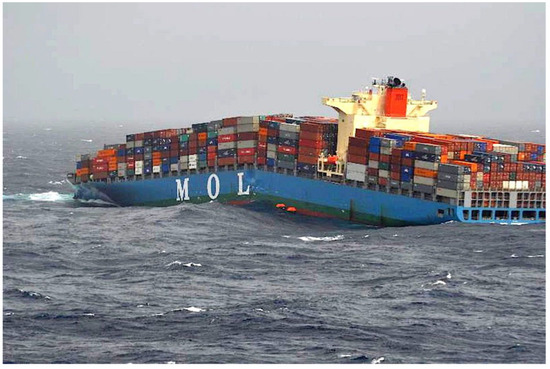
Figure 30.
Breakup of the container ship MOL Comfort, off Yemen, in June 2013. Photo from [109] with permission; originally taken by Mitsui O.S.K. Lines, Ltd., Tokyo, Japan.
Global wave models, such as those run by NOAA, ECMRF, the US FNMOC, and other major organisations, assimilate observational data from satellite-borne altimeters and other sources into sophisticated computer code implementations of the fundamental equations that govern the kinds of processes illustrated in Figure 16. Wave and swell now-casts and forecasts produced by these models are widely available on spatial resolutions variously in the range 16–30 km, but it is fair to say that these products are ‘model rich but data poor’. In particular, the swell forecasts that are available to optimum routing services rely on a high degree of extrapolation from models because the primary source regions are typically thousands of miles away, and swell attenuation data is hard to acquire from normal technologies [110,111]. In addition, estimates of the bandwidth of the swell are seldom available. Yet swell makes up more than 50% of the total wave energy over much of the world’s oceans and is the greatest threat to ship stability. Thus the ability of HF radar, under good propagation conditions, to measure the period, direction, and amplitude of the swell is a highly valued attribute. The relevant theory was reported in [112].
Another key task in ocean routing is to guide ships around storms. In the interests of safety, and the presence of many uncertainties, conventional procedures, and common sense implies that conservative measures should be adopted. In addition to delivering accurate real-time location and mapping of wave height in storms, skywave radar-generated high-resolution wave directional spectrum data would enable vessels to avoid making unnecessarily wide diversions around an area of storm activity, whilst keeping longitudinal and torsional stresses to acceptable levels.
A related issue that emerged with the advent of container ships is the loss of containers due to rough seas. This does not have to be associated with the loss of a ship, as illustrated in Figure 31. To illustrate the scale of the problem, one recent report announced that 3000 containers had been lost overboard in 2020 and a further 1000 in the 90-day period up to March 2021 [113,114]. Explanations for this trend are routinely identified but seldom acted upon. The dangers range from stevedores incorrectly locking boxes on top of one another to captains not deviating from a storm so as to save on fuel and time as they face intense pressure from charterers, according to the IMO [115].
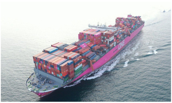
Figure 31.
The ONE Apus arrives in Kobe, Japan, on 8 December 2020 after losing an estimated 1816 containers overboard, approximately 1600 nautical miles northwest of Hawaii, USA. Photo courtesy W K Webster and Co. Sidcup, UK.
Apart from the immediate financial loss, containers can stay afloat for days or even months, posing a serious hazard to shipping. The IMO’s Maritime Safety Committee has initiated a container loss reporting scheme, in the hope that it will enhance the positioning, tracking, and recovery of such containers [116]. Detecting and tracking them as they lie almost completely submerged might seem a challenge beyond the powers of HF radar, skywave, or surface wave, but there is a possible solution. To fit compliant transponders or GPS-fitted beacons reporting to satellites would be prohibitively expensive, but a cheap, simple, robust, compact, passive device based on a design used in HF radar experiments could be built for less than USD 100 and attached/removed in an instant. The implementation details for this device are still commercial-in-confidence but the principle has been described in [117].
While some other sensing technologies provide positional information on large, slowly-developing storms, together with reasonable estimates of severity, there are more localised intense weather systems in the form of tropical convective cells that are not detected by those sensors. These are born, evolve, and die within the space of perhaps two hours, and while they do not approach the scale or strength required to threaten large ships, the heavy rain and very strong winds can cause serious discomfort and danger for smaller vessels, such as most of the world’s 3.7 million fishing boats [118]. Skywave radar has demonstrated the ability to detect the development and decay of these short-lived events [84]. Figure 32 shows how the radar signature of a convective cell varied over two hours spanning one such event. At the end of the event, the sea clutter spectrum can be seen to have returned to its pre-event form, after more than 20 dB enhancement in 30 min as the cell developed.
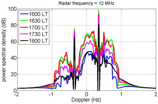
Figure 32.
Sea clutter Doppler spectra computed from raw buoy measurements of wave spectra during the lifetime of a convective cell near Bathurst Island, Northern Australia. Noise in the buoy measurements is reflected in the Doppler spectra, but the transient and return to the pre-event state are unmistakable.
Protecting against hazards is not the only way that skywave radar can assist shipping. We have mentioned that route planners try to take advantage of favourable ocean currents, and presumably avoid opposing ones, to save fuel costs and increase speed over ground. Ocean currents can be mapped in far greater detail and with higher spatial coherence using skywave radar than is possible with buoy networks and other practical technologies. East–west equatorial currents have speeds around 0.7 ms−1 while Western boundary currents reach speeds of 2.5 ms−1 so precise knowledge of the current vector map is of crucial importance. This is illustrated in Figure 33, which shows a meridional transect of the current over a region in the Pacific Ocean [119]; we can see that the north-south gradient of the flow is very high at some latitudes.
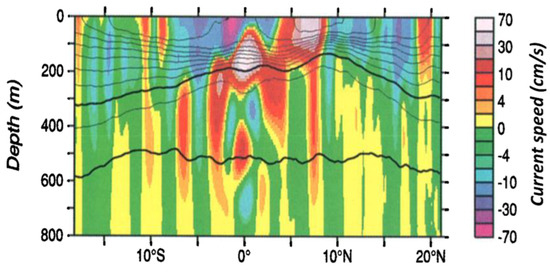
Figure 33.
A meridional transect across the Pacific Ocean plotting zonal current speed; rapid speed changes are evident at some latitudes [119].
One might think that large-scale ocean currents are stationary and, hence, trivially incorporated in the models used for route design. In reality, this is not strictly true for large-scale currents, as meaningful fluctuations can occur on a timescale of a month or less, and it is certainly not true for finer scales, because the oceans are dotted with mesoscale eddies—the dynamical equivalent of weather in the atmosphere, as pictured in Figure 34.
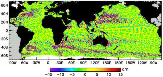
Figure 34.
A snapshot of the spatial distribution of strong mesoscale eddies. Note the dominance of eddy shedding by western boundary currents.
Mesoscale eddies are vortices that peel off from the main oceanic boundary currents. The vortex structures can be either cyclonic or anticyclonic; they exist over a wide range of radii, with most energy concentrated in the band 10–500 km. They extend downwards typically 100–1000 m and have a mean lifetime of about 32 weeks, during which they travel a mean propagation distance of 550 km, a mean drift speed of 0.03 ms−1. However, drift speed is not so much the issue as the circumferential current speed, which can approach 1 ms−1, though more typically it lies in the range of 0.1–0.5 ms−1. This can easily add or subtract 10% of a vessel’s speed over the ground, so any ability to track these structures and exploit them for ship routing would be highly valuable.
Many ocean climate models have horizontal grid-spacings that are too coarse (typically 1° ⪝ 110 km) to explicitly represent any but for the very largest eddies, and even in newer climate models, the grid-spacings (typically ¼° ⪝ 30 km) are said to be only “eddy permitting”. The eddies are conventionally detected and tracked by satellite altimetry, as the core depression/elevation may exceed 45 cm, while the precision of altimeters now approaches 1 cm. An example of an altimetric map of the eastern Indian Ocean is shown in Figure 35, along with the inferred geostrophic current velocity [120].
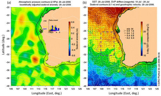
Figure 35.
Altimeter map of the eastern Indian Ocean, 26 July 2006 [120]. (a) Sea-level anomaly, (b) geostrophic velocity. The purple box marks the area selected for detailed modelling, as presented in Figure 36.
The altimeter samples lie on one-dimensional tracks and revisit times may be long, so the reconstruction of an elevation map is not truly synoptic. Moreover, current speeds are derived via models, not measurements, so these economically important ocean features are not well captured by spaceborne sensors.
In contrast, skywave radar is both synoptic and persistent. Some existing radars can achieve a resolution cell size as small as 1 km × 10 km at a range of 1000 km, so, providing the ionospheric propagation conditions support adequate Doppler sensitivity, HF radar mapping of mesoscale eddies is feasible, just as it is with HFSWR at shorter ranges (see e.g., [121,122]). To demonstrate this, in Figure 36 we have taken the small region within the rectangle superimposed on Figure 35, synthesised the current field (see Figure 36a), and then computed the Doppler map that a skywave radar at a specified location (Laverton in this instance) would produce (Figure 36b). The ability of the radar to discern the structure of the eddy field is evident, as is the precision of the current measurement.
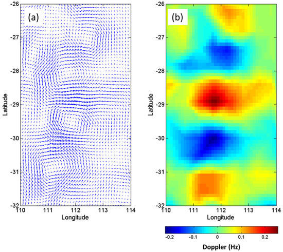
Figure 36.
(a) The synthesised current field within the rectangle shown in Figure 35, sampled at a higher resolution than shown there. (b) The corresponding radial current speed map as it appears to a single radar.
Even in moderate seas, the waves have a significant impact on ship performance because the ambient waves increase the resistance against which work must be done. Specifically, in addition to frictional loss and wave resistance (generation of the wake) that apply in calm water, there is a significant interaction between the ambient wave field and the dynamic response of the ship as it heaves, pitches, and rolls; apart from this ‘radiation’ mechanism, there is also a reduction in the efficiency of propulsion as the flow incident on the propeller departs from laminar.
It is thus rather obvious that waves perturb ship motions and degrade vessel performance, so the optimum routing should take the waves into account. Far less appreciated is the fact that the same is true for the wind forces acting on a ship. Is this effect significant? We can obtain a crude estimate as follows. For a ship’s speed and a following (tail) wind speed , the wind load is given by so the power delivered to the ship is , where is the presented area, is the density of air, and is the drag coefficient. The largest container ships can exceed 60 m in beam and a similar amount in height when laden, so the area presented to the following wind—the windage—is ~3500 m2.
For a ship speed of 20 knots and a wind speed of 30 knots, the power delivered in this case is ~0.54 MW, compared with ship power of 40–60 MW at normal cruising speed (and the maximum of around 80 MW). So, the tailwind contributes only about 1%, to the ship’s advantage. However, for a headwind, the work done by the wind against the ship motion is ~29.6 MW, so half the ship’s power must be expended overcoming the wind. The consequences of a beam wind, acting on the far larger area presented to port or starboard, can clearly be enormous.
Now, in these calculations, we have ignored the aspect dependence of the drag coefficient. For the tailwind case, a stern aspect, , seems reasonable, as the drag coefficient of a flat plate is 1.28. From a forward view, as pictured in Figure 37, the drag may be slightly less, depending on the loading, but as ball-park figures, these numbers show the huge pay-off that can come from avoiding headwinds. HF skywave radar is the ideal source of that information. At the same time, we should not overlook the effects of winds on ship dynamics and load stability, so real-time maps of the surface winds and especially sharp transitions in the wind speed and direction have huge operational utility.
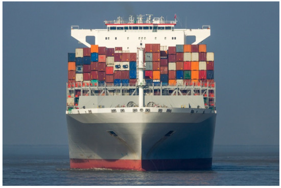
Figure 37.
The profile of a large container ship from a forward view. While the angled hull presents a lower drag coefficient, most of the above-deck structure and load offer high resistance.
To have a feel for the way different considerations impact the optimum ship routing, we constructed a simple model. In the approach, we have adopted, the cost function consists of three elements: a local (point-wise) measure of inefficiency that is integrated over the entire route, and a set of constraints that apply to the global solution. To illustrate, we started with the significant wave height map extracted from the radar data used to generate the wind direction map shown in Figure 19 and used this surface as the penalty per kilometre travelled. The surface is plotted in Figure 38, together with a scenario and some solutions.
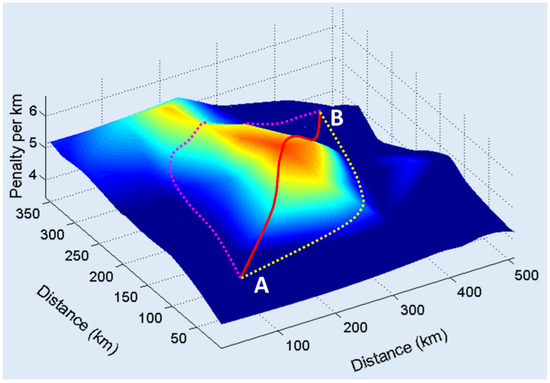
Figure 38.
An example of optimum ship routing. The great circle route between two locations A and B on opposite sides of a storm is shown in red, while two more efficient routes are shown in magenta and yellow, though only the magenta route satisfied all constraints.
Obviously, this is a very simplistic measure, for all sorts of reasons, but it serves our initial purpose. We then imposed the global hard constraint that the journey from A to B should take a specified time and added a separate soft constraint in the form of a negative penalty (‘benefit’) function that rewarded uniformity of progress. To find the extrema, we adopted the eugenics-modified Pareto genetic algorithm reported in [123], which is used for many HF radar optimisation studies. Figure 38 shows three possible routes: the Great Circle path (red) a fast route that fails the hard constraint (yellow dots), and a reasonably steady route that met the hard constraint (magenta dots). This rather trivial model in no way compares with the expert route service methodologies but playing with it has helped us understand the relative importance of different considerations.
4.2.2. Fishing
The total number of fishing vessels in the world has been estimated at several million, with more than 68,000 longer than 24 m and equipped to operate in the deep ocean.
Many of the issues that we have discussed in the preceding subsection apply to the fishing industry, so we shall not repeat them here. The most obvious differences lie in the relative importance of wind waves as opposed to swell because of smaller vessel size, and the nature of fishing operations. Increasingly, fishing fleets venture far from their home ports, as local fish stocks become depleted.
In view of the long transit times, often longer than the time spent on location fishing, the fishing vessels have a priority need for accurate and timely data on wave height and direction, especially high sea states. Schedules are not so tight as with cargo fleets, so gaining a few percentage points in speed over the ground is inconsequential, with safety a far greater concern; in any event, budgets seldom allow for recourse to advanced route planning. If skywave radar data were available, it would be of high utility.
There are eight major types of commercial fishing vessels of which three—trawlers, seiners, and longliners—dominate the deep ocean fleets [124]. The different techniques employed place different demands on the deployment of equipment and its retrieval with the catch, so the needs for sea state information at the location and the acceptable ranges of suitable fishing conditions also vary. Trawlers, the most common class, are particularly sensitive to the conditions, with many boats lost each year hauling in the nets, so synoptic-scale directional wave spectrum data and real-time notification of changing conditions would be of great value.
A less obvious but more time-critical type of information is knowledge of the position, geometry, sea surface anomaly, and direction of rotation of mesoscale eddies in the accessible fishing areas. Not from their dynamics, which as we have noted, are relatively benign, but because they can harbour concentrations of fish. This comes about because, when the peak orbital speed exceeds the bulk transport velocity, eddies are essentially closed systems that advect their contents as they migrate. During cyclonic eddy formation (counter-clockwise in the northern hemisphere), the divergence of surface currents (due to the Coriolis effect) leads to upward doming of isopycnal surfaces, leading to upwelling of cold, nutrient-rich water to the nutrient-poor upper layers, stimulating phytoplankton production [125,126]. This, in turn, promotes fish larval population growth by counteracting starvation and predation, leading to higher concentrations of the fish species than are found in the outside ambient waters. At the boundaries, where local turbulence mixes the two water masses, warm water species such as squid, swordfish, and tuna gather to take advantage of the enhanced food density [127,128,129,130,131,132]. Other, smaller species prefer cold water concentrated in the core, so the target fish type determines the best location for fishing. This distribution has been exploited by a few well-informed fishing fleets, able to access the eddy data, but existing sources lack adequate resolution. One expert has expressed the requirement as a metaphor: “You can move from a desert area to a rainforest within a few kilometers” [133]. In the present context, we see that skywave radar could certainly augment and enhance other sources of information on eddies and their intensity [134]. Even more importantly, the problem of advising a fishing vessel is one of relative position, not absolute position. As a radar can detect both the boat and the current filamentary structure, it can provide vectoring information irrespective of ionospheric irregularities that make absolute coordinate registration difficult.
A map showing fishing activity worldwide, as estimated from AIS data in 2016, is shown in Figure 39 [135]. The AIS collects information transmitted from cooperating vessels via satellites and shore-based receivers and provides this to users around the world. Unfortunately, the data is often less than perfect—the shipboard devices may be faulty or incorrectly used, they may be deliberately manipulated to report false data including ship identity as well as position, satellite reception may be poor, errors can occur due to overloaded communication channels when the ship is in very crowded waters, and so on. Most commonly, in the case of fishing fleets, boats violating sovereign zones or protected reserves attempt to conceal their presence by deactivating their AIS devices. As a further step to remaining unreported, they may stay outside boundaries during the day, perhaps supported by a mother ship, but enter the forbidden area at night.
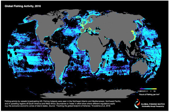
Figure 39.
Fishing activity as defined by those vessels that report their positions continuously via AIS [135].
4.2.3. Military
From the defence perspective, skywave radar has an enormous amount to offer, most immediately by generating and maintaining a recognised air picture (RAP) and recognised surface picture (RSP). Based on this type of situational awareness, specific tasks can be undertaken, including target classification and over-the-horizon targeting. Many other missions can be addressed, some rather subtle, but we shall not explore this subject here.
4.2.4. Offshore Oil and Gas Industries
The offshore structures that house oil or gas extraction facilities are designed to survive high winds and sea states, as prevail in the North Sea and the Gulf of Mexico, for example, so the direct impact of moderately inclement conditions is felt mainly in the construction phase and during off-loading and replenishment. However, for those facilities in hurricane-prone regions, the likelihood that a severe event is in prospect has serious consequences: drilling operations must cease, chemicals must be injected into each well to stabilise the temperature and pressure of the rig, underwater plumbing may need to be retracted or detached, and the crew may need to be evacuated. Some modern drilling platforms are not rigidly anchored, especially in deeper waters, and so have some degrees of freedom to pivot and move out of harm’s way, but to do this safely requires detailed oceanographic and wind information, including forecasts and warnings over a time scale of days.
It follows that having persistent skywave radar data to provide greater detail than available from satellite sensors has significant potential for minimizing loss of production and risk of major damage due to severe weather. In particular, knowing the spatial distribution of the strongest waves can enable operators to decide whether to ride out a storm, thereby saving millions of dollars, rather than closing down, which imposes a minimum recovery time of several days. The flexibility inherent in skywave radar tasking means that it can be directed to focus attention on a facility facing a severe threat and to share its real-time information with rescue services if required.
There is another important contribution that skywave radar can make to offshore extraction facilities: the detection of impending internal waves. The density stratification of the ocean due to temperature and salinity variations introduces the possibility of waves propagating along the main density layer boundaries, and these internal waves have astonishing properties. While they move more slowly than long surface gravity waves, their amplitudes can be immense—over 150 m. Moreover, the rate of change of the current profile is astonishing, as we have reported [83] and illustrate in Figure 40. Each of the eight time-stamped panels shows (i) on the left, the horizontal current vector measured at seven stations along a vertical line from the water surface to the bottom, at a depth of 225 m, and (ii) the water temperature measured along a vertical chain of thermistors.
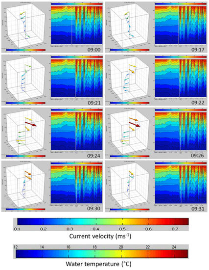
Figure 40.
A 30 min time series of current and temperature profiles recorded by in situ sensors during the passage of an internal wave. The grey vertical line indicates the time of the sample; only the first cycle of the internal wave is sampled here. The axis labels are too small to read in this mosaic, so we explain them here. The vertical axis is depth, spanning 225 m from the sea floor to the sea surface. The horizontal axes measure current velocity components, spanning ± 0.75 ms−1. The colour bar beneath the current vector ‘boxes’ calibrates the current arrows, spanning the magnitude range 0–0.75 ms−1. The other colour bar, above the temperature histories on the right of each panel, spans the temperature range of 12–25 °C. Both colour bars are reproduced below the main figure.
The passage of the packet of internal waves is vividly displayed by the displacement of the water as revealed by the temperature profile, with nine cycles of the wave packet visible. For offshore oil, gas, and mining activities, the current shear is important [136]. As evident in the panels on the left of each frame, the associated currents result in strong and rapidly varying vertical gradients in horizontal stress on any immersed structures, and these shear forces can tear apart drill pipes and risers, and even damage the cabling that moors large platforms. Figure 41 shows a drilling platform in the Andaman Sea being tilted by 3° during the passage of an internal wave.
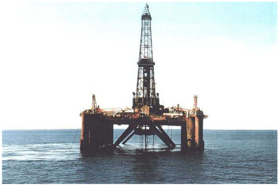
Figure 41.
An offshore platform in the Andaman Sea, tilted by 3° during the passage of an internal wave. Much of the tilt is into the plane of the image.
The challenge of detecting internal waves lies in the fact that the associated surface displacement is tiny, revealed mainly through a slight modulation of the ambient surface waves. While the approximate distribution of large internal waves can be estimated since the strongest ones are generated by tidal flows over bathymetric features, the variability is far too great to allow confident prediction, so a technology that can detect and track the waves has obvious applications to offshore structures. Skywave radar has demonstrated the ability to detect these large internal wave packets at ranges in excess of 1500 km [83]; an example is shown in Figure 42. As the platforms have their own echo signatures, the relative position of the internal wave peaks to the platform, and the speed of advance can be measured quite accurately.
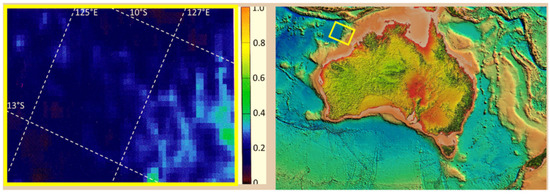
Figure 42.
Internal wave signatures of internal waves crossing the continental shelf. In this case, only the modulation of wave height is shown, but other more sophisticated signatures can be retrieved.
4.2.5. Science
The high dynamic range of modern skywave radars, and some surface wave radars for that matter, provides a window onto many physical phenomena that are extremely difficult to investigate with other sensors. One example is the study of nonlinear hydrodynamic processes in the ocean environment, such as the Benjamin–Feir instability and Fermi–Pasta–Ulam recurrence. A second is the investigation of wave growth and decay as source terms in the Hasselmann equation for wave spectrum evolution. Yet another is concerned with establishing the radar signatures of conditions that are conducive to the formation of rogue waves. There are many more. Moreover, we need not restrict ourselves to oceanographic phenomena: skywave radar is an outstanding tool for studying ionospheric structure and dynamics, including the propagation of acoustic-gravity waves, geomagnetic disturbances, plasma instabilities, and a host of other geophysical processes. The knowledge gained from such investigations applies to HF communications and shortwave broadcasting, not just to skywave radar.
4.2.6. Deep Sea Mining
The global appetite for mineral resources continues to extend the footprint of extraction industries [137], with the deep-sea floor—the areas below 200 m depth—now the subject of exploration to assess the size and characteristics of mineral deposits, together with preliminary research and development of practical mining techniques [138,139,140,141]. All activities are required to conform to arrangements and contracts laid down by the International Seabed Authority, a body established through the UN Convention on the Law of the Sea that governs deep seabed mining [142]. More than 1.5 million km2 have been marked for mineral exploration in the Pacific and Indian Oceans, and along the mid-Atlantic Ridge. The geographical distribution of these activities is shown in Figure 43. Needless to say, there are more voices urging caution with the idea of deep-sea mining, rather than promoting it (see e.g., [143,144,145]), yet already operations are underway off the coast of Namibia and Papua New Guinea. The area of greatest concern to environmentalists is the Clarion-Clipperton Zone (CCZ), a region of some 4.4 million km2 in total. Companies and national bodies from at least seventeen countries plan to deploy robots and vacuum hoses to raise mineral nodules and sediment from the sea floor, filter and extract the valuable elements, then discharge the slurry back into the sea. The consequences for benthic habitats could be catastrophic. Studies of benthic plume dispersal suggest relatively localised zones of contamination from the dredging itself [146], but others focusing on the entire extraction process argue that, instead of sinking rapidly, the slurry may be carried hundreds or even thousands of kilometres, doing untold damage to marine ecosystems.
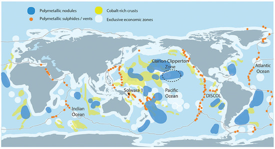
Figure 43.
Map showing the locations of the three main marine mineral deposits: polymetallic nodules (blue); polymetallic or seafloor massive sulphides (orange); and cobalt-rich ferromanganese crusts (yellow). Reproduced from [139] which in turn drew on [137].
It is easy to imagine prospective tasks for skywave radar, either to assist the mining activities by providing synoptic scale, high-resolution directional wind and wave spectrum data and currents so that safe operations can proceed, or serving in a regulatory monitoring role, assessing the Lagrangian transport of the slurry by ocean currents, Ekman transport, and the Stokes drift so that the ISA can demand that mining cease while threatening conditions prevail. Of particular value would be information about the direction of sediment transport through the entire water body, since this type of pollution affects fish populations at all depths. No remote sensing technology can provide a comprehensive picture, but multi-frequency radars routinely observe the effects of current shear, while theoretical studies suggest that HF radar can measure the surface signatures of shallow sub-surface flows, even when the direction varies with depth. The present state-of-the-art is limited to sampling the dispersion relation as inferred from the first-order Bragg peaks, based on the assumption of unidirectional, depth-varying flow, but a study now underway is exploring the signature manifested in the second-order spectrum for an arbitrary shear flow [35]. Irrespective of the feasibility of this approach, HF radar is unique in that it can provide synoptic, persistent, near real-time maps of the ocean current ‘weather’ taking account of mesoscale eddies and, hence, the upper layer transport of mining slurry.
4.2.7. Search and Rescue
When an accident occurs at sea, there is often a long delay before rescue and recovery units arrive at the location. During this interval, wave action and currents may have transported and dispersed survivors and flotsam, with the consequent risk of loss of life and property. Timely and accurate guidance is essential to the prosecution of search and rescue missions. If the entity to be rescued is of sufficient RCS, it may be detected directly by HF skywave radar; in this case, the radar can vector rescuers to the target’s present location. If not, then the radar can use its remote sensing capabilities to predict how the entity has moved under the agencies of wind, waves, and currents.
To illustrate the possibilities and the challenges of tracking floating objects over extended periods, we cite the experiments carried out by SRI using the WARF radar in 1974 [147]. Figure 44 shows the track of a buoy fitted with a transponder to increase its effective RCS; it was tracked for four months in the North Pacific, at ranges up to 3100 km. Similar experiments have been conducted on a much smaller scale using HFSWR systems [148], but no other skywave radar demonstrations have been reported.
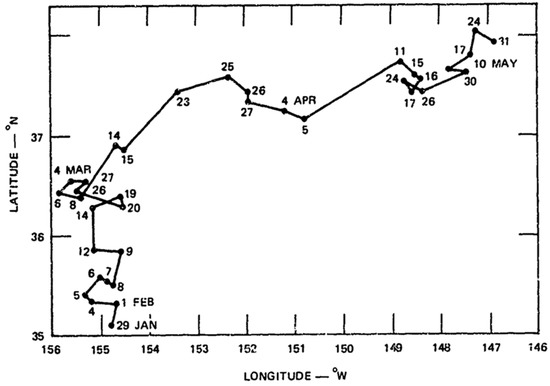
Figure 44.
WARF skywave radar track of a buoy fitted with a repeater recorded over four months in 1974; note the rapid changes in direction and loops [35].
For a mid-ocean accident, rescue vessels may not reach the scene until 48–72 h have elapsed, by which time survivors may have drifted up to 100 km. The requirements for successful search and rescue are highly demanding, as visibility of floating objects in rough seas is greatly reduced, and the multiscale nature of the local forcing renders standard ocean current charts, as used by navies and merchant shipping, almost useless. If one is to predict the net displacement, one must consider the effects of the prevailing conditions, taking into account all the principal transport mechanisms—currents, Stokes drift, wave forcing, Ekman transport, windage response—and these integrated over the elapsed time, during which changes may have occurred [149,150,151,152,153,154]. HF radars of all configurations can, in principle, address most of these effects, subject to ionospheric propagation conditions, and the wide-area surveillance attributes of HF skywave radar are ideally matched to the task of narrowing the search volume.
We also point out that, unless the rescue agency is made aware of the wind and sea conditions in the vicinity of the accident, and all along the route, inappropriate resources may be dispatched, and further lives placed at hazard. Moreover, if a ship fails to arrive at its destination, but no SOS has been received, only skywave radar has the wide area coverage, persistence of surveillance, recorded detection and track history, and sensitivity to changes in vessel behaviour to be able to look back at the traffic history, and identify the location of some irregularity of behaviour, perhaps even diagnosing the cause of the mishap. A skywave radar observing the sinking of the Titanic would have detected the presence of icebergs in the area close to the ship and then the sudden change in ship motion.
4.2.8. Coastal Damage, Cyclone, and Tsunami Warning
We shall interpret this category in a somewhat more general way than Rhodes and Chadwick, by considering the impact of tropical cyclones, commonly termed hurricanes in the Atlantic and eastern Pacific, and typhoons in East Asia. The energetics of these severe weather systems is governed by the exploitation of latent heat and the dynamical influence of the Coriolis force. Together, these dictate the global distribution of cyclones to be that shown in Figure 45.
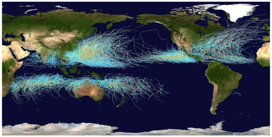
Figure 45.
NASA map of the cumulative tracks of all tropical cyclones during the 1985–2005 time period [155]. Track colour indicates storm intensity.
Skywave radar has a long history of mapping tropical cyclone wave fields [71,76,156,157,158,159,160], and we have already shown examples of radar products in Figure 18 and Figure 20, the former showing significant wave height and the latter wind direction of Tropical Cyclone Victor in March 1986. This kind of radar-derived wind information, together with the amplitudes, frequencies, and directions of propagation of waves being generated by the storm, can be provided in real-time to agencies responsible for issuing warnings and taking measures to minimise harm.
Even more importantly, the synoptic coverage of skywave radar enables forecasters to gain improved estimates of the steering current. Tropical cyclones are steered by several forcing agents, notably the mid-tropospheric winds around sub-tropical highs, not as pure advection but in a dynamical interaction, as well as ocean currents and sea surface temperature. The stronger the cyclone, the deeper the layer of the atmosphere that applies the forcing. Now, over the oceans, much of the information about winds comes from satellite imagery via the extraction of cloud motion vectors which, combined with other information and interpreted by experts, yield estimates of the atmospheric motions at cloud height. Owing to intrinsic cloud pattern asymmetry and vertical wind shear, the apparent centre of cloud signatures of specific meteorological events taking place at sea level may be displaced horizontally by significant distances, leading to erroneous forecasts of cyclone position and steering direction. In order to locate the true position of the cyclone eye at sea level, HF skywave radar researchers introduced a quantity called prospective vorticity, computed from the measured direction of the short gravity waves excited by the cyclonic winds with an adjustment to allow for latency in the ocean response to the wind stress. This also provides a measure of the vertical wind shear and, thus, facilitates superior estimation of the steering current, predicting where the cyclone may make landfall.
Figure 46 shows an example, using data from Tropical Cyclone Chris in 2002. The map plots prospective vorticity; the national weather service estimate of the cyclone eye position derived from cloud imagery is marked. There is a residual error/displacement of some tens of kilometres, which is a significant distance from the forecaster’s perspective.
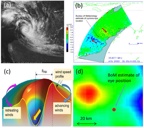
Figure 46.
Prospective vorticity analysis of Tropical Cyclone Chris, 2002. (a) Composite VISSR image of TC Chris on 4 February 2002, (b) Jindalee skywave radar map of radial current speed, (c) model of the wind speed asymmetry about the direction of motion, (d) map of prospective vorticity showing the discrepancy between cloud-based location as derived by the Australian Bureau of Meteorology and the peak value of prospective vorticity.
A more subtle contribution of skywave radar to cyclone monitoring was demonstrated in 1984 with the system designated Tropical Cyclone Pancho, in the northeast Indian Ocean, on account of a spiral cloud structure observed by TIROS-N. As the Jindalee radar was available at the time, a radar-directional surface wave field map was generated, revealing that there was no closed vortex signature in the wind-generated wave field at the surface. TC Pancho was subsequently demoted to tropical depression status, and costly re-routing of ships and precautionary shut-down of offshore facilities was avoided.
A different type of threat is posed by tsunamis. The use of HFSWR to provide early warning is well established, but the same task can be carried out by skywave radar, over far greater areas. For both HF radar configurations, the principal signature is that of advection of the Bragg-resonant waves, usually detectable only when the tsunami waves reach shallow waters, but several other candidate signatures are only accessible to skywave radar, as reported in [48,49,50,51]; some of these could increase warning time substantially in locations where the continental shelf is narrow.
4.2.9. Recreation
Recreational activities in the maritime domain constitute a vast industry but they tend to be concentrated in coastal zones where forms of surveillance and environmental monitoring other than skywave radar can be accessed. Of course, weather forecasts for remote areas can benefit enormously from the assimilation of skywave radar data, as was done in Australia from 1983 to 1995 [13], but direct input to recreational services is rare. Nevertheless, there are several roles for skywave radar that have been invoked on occasion. One, which had no counterpart with other sensors was the task of monitoring the entrants in an international yacht race, the Darwin to Ambon Race, which was held in August each year from 1976 until 1998 when unrest developed on the Indonesian island. During August, strong and steady southeast trade winds prevail, making for excellent sailing on the northbound route. Seizing opportunities between conducting other radar missions, the Jindalee radar was able to track the yachts intermittently as they crossed 1000 km of the open sea, to a range of 2300 km. There are a number of tools that facilitate the detection of small vessels, including an understanding of sailing techniques, real-time access to the radar measurements of the wind and the prevailing directional wave spectrum, knowledge of the radar scattering properties of the boat, and the ability to adapt waveform and signal processing algorithms according to propagation conditions and boat dynamics. The signal-to-clutter ratio (SCR) achievable at one stage during the 1985 race is shown in Figure 47 where it is plotted as a function of radar frequency and bistatic angle, under the prevailing conditions and assuming ideal propagation conditions. The directional spectrum was retrieved from the sea clutter spectrum and combined with the known RCS of a typical yacht as a function of radar frequency to compute the SCR. Of course, the radar used for that experiment had no bistatic degree of freedom, so it could not access the optimum configuration.
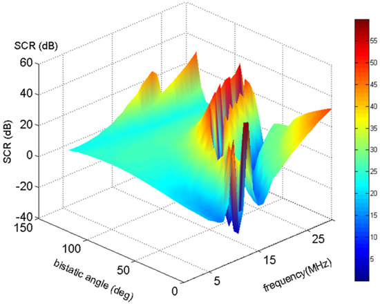
Figure 47.
The signal-to-clutter ratio measures the detectability of ship echoes and varies strongly with radar frequency and the bistatic scattering geometry. This kind of radar-generated display can be used more generally to advise a network of OTH radars on how to optimise resource allocation.
Tourism, in the form of cruise ships, could, in principle, take advantage of skywave radar measurements of wind and sea conditions, though these vessels are usually fitted with stabilisers so only very rough seas affect passenger comfort and safety.
4.2.10. People Smuggling and Illegal Immigration
A problem that scarcely registered at the time of the Rhodes and Chadwick report [101] but is of enormous concern today is the illicit transport of human beings with a view of bypassing legal entry procedures. Under the United Nations Convention on the Law of the Sea (UNCLOS), a nation’s territorial sea extends to 12 nautical miles from a formal baseline. Ships of any nation have the right to innocent passage through other nations’ territorial waters, but not the actions that are involved when delivering illegal entrants. Beyond this lies the contiguous zone, extending to 24 nautical miles, provided for the purpose of administering the territorial sea, and then nations have rights to an Exclusive Economic Zone extending to 200 nautical miles. Often the challenge with an illegal entry is the detection and interception of the offending vessels before they enter national waters, but in order to achieve the latter, much earlier detection is essential.
Although some countries employ their military naval units to police their national waters, others provide a Coast Guard or similar entity, which may lack the surveillance resources available to the navy. Further, the number of vessels allocated to this function seldom comes close to what is needed to be effective without extensive cueing from external agencies. HF radar is well suited to this task; an unpublished study of the possible use of HFSWR in the Mediterranean indicated a high level of capability in some key areas [161]. However, once the range band of interest exceeds 50–100 km, HFSWR offers much-reduced performance, and, over a long coastline, the number of such radars becomes impractical. The desirability of detecting boats at much longer ranges can be addressed only by air or surface patrols, advanced spaceborne sensors, or skywave radar. Several countries have carried out comparative cost analyses of the competing technologies; in every case, skywave radar was the most efficacious when measured by the metric of cost per detection per unit area per unit time.
That said, all of these options have limitations. The detection of very small boats such as inflatables is very challenging for skywave radar and may be described as an art as much as a science, drawing on a wide range of disciplines and sophisticated radar design. To complicate matters, the illegal boats may exploit expert knowledge to minimise the probability of detection, though generally, the nature of the vessels offers limited scope for this. One can argue that, realistically, such small craft are unlikely to have sailed across the open seas beyond the EEZ, but that reasoning ignores the degree of desperation in some regions.
In summary, skywave radars have been tasked with the mission of detecting boats attempting to deliver illegal migrants, and indeed, have successfully performed this mission, but one might hesitate to build a radar solely for this purpose.
4.2.11. Intrusion of Foreign Fishing Vessels
Exclusive economic zones are difficult to police, as we have noted, but the nature of fish poaching makes it relatively easy to monitor. Often a mother ship stays beyond the EEZ while smaller craft are sent into the zone to catch the target species, hoping to escape to the open sea if spotted by an aerial patrol or similar. Thus two features are common—first, a loitering, rather substantial vessel that is easily detected, at a well-defined range, so searching is essentially a one-dimensional task, not two, and second, smaller vessels whose movements and, hence, Doppler signatures are characteristic of the kind of fishing being undertaken. Of course, the national powers of jurisdiction and rights of seizure are a separate matter altogether, but skywave radar can certainly carry out the mission, provided that ionospheric propagation conditions are not particularly adverse.
4.2.12. Offshore Wind Farms
The proliferation of offshore wind farms is continuing and likely to accelerate as renewable forms of energy replace fossil fuels. Most of the wind turbines presently in operation are fixed to the sea floor on solid foundations, at great cost, with significant impact on the benthic environment, and limited to waters less than 50 m deep. A recent development was the introduction of floating wind farms—the first commenced operation in 2017 in the North Sea—which is tethered to the sea floor by mooring lines. In this case, the depth can exceed 200 m [162]. This opens up vastly more areas for deployment, which is doubly attractive because the winds tend to be stronger further offshore. It has been estimated that 80% of potential wind power is to be found in these deeper waters [162]. A side benefit is a much-reduced impact on marine habitats.
Wind turbines must turn to face the wind and apply pitch control to optimise power output under the prevailing conditions and to avoid damage. This adaptation occurs on a shorter time scale than the ocean surface changes that can be sensed by skywave radar, so the main contribution that radar can have as far as wind is concerned is to provide early warning of severe conditions heading towards the facility. A highly significant contribution that can be made is with the regional mapping of waves and currents, as these determine the forces on the platform and the mooring. Whether the wind farm towers are deep water tension leg platforms (TLPs) or gravity-based structures (GBSs), it is imperative to keep their natural frequencies away from those of any exciting forces. Given the wave climatology for the installation area, TLPs are designed to keep their natural frequencies in heave, pitch, and roll degrees of freedom at several times the expected dominant wave frequency, whereas natural frequencies in surge, sway, and yaw degrees of freedom are designed to be lower than the dominant wave frequency. A GBS will have its natural frequency well above the dominant wave frequency. Thus, linear resonance with the fundamental component of ocean waves is avoided, but ocean waves are hydrodynamically nonlinear, so they possess bound harmonics. Strong interaction with these higher frequency components, especially the second and third harmonics, is all too possible, creating a degree of risk of a dangerous platform response. HF radars possess the unique ability to detect and measure the amplitude of the bound harmonics of the Bragg-resonant waves and, thus, alert the wind farm operators to an approaching threat. Advanced platform design would include the ability to reduce platform response by altering platform resonant frequencies and applying damping, given sufficient warning. Accordingly, HF radars would be integral to supporting an adaptive response functionality, with skywave radar able to support the deep-sea platforms beyond the range of HFSWR.
4.2.13. Sovereignty Violation
There is a school of thought—put into practice in some marine areas—that regular use of a patch of ocean for other than normal transit will, in time, entitle the frequenter to claim ownership. The construction of artificial islands may accompany such an undertaking. HF skywave radar can provide a continuous, quantitative record of air and surface activities over a region that could become a source of contention, thereby establishing a basis for legal procedures if required.
4.2.14. Piracy and Sanction-Breaking
It can come as a surprise to learn that piracy on the high seas, and some not-so-high, is far from uncommon. Figure 48 shows the distribution of significant acts of piracy over the past 40 years [163].
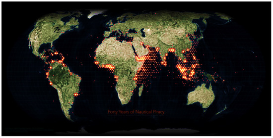
Figure 48.
A map showing the distribution of marine piracy events over a forty-year period [163].
4.2.15. Oil Spill Detection and Tracking
Oil spills at sea have decreased markedly over the past three decades but, even so, there were 63 oil spills of 7 tonnes and over between 2010 and 2020, resulting in 164,000 tonnes of oil lost; 91% of this amount was spilled in just 10 incidents. Over the same period, the incidence of illegal tank flushing when out of sight of coastal monitoring systems has undergone a similar decline, due in part to fear of detection by spaceborne monitors, linked to AIS data. It seems reasonable to conclude that any oil spill detection capability of skywave radar is less relevant today than in the twentieth century when hundreds of thousands of tonnes of oil were being lost at sea each year [164]. In any event, spaceborne SAR and satellite optical instruments do a far better job of detecting oil spills than might HF skywave radar, but it is interesting to observe that the presence of surfactants such as oil spills, seaweed, and algal blooms does present an HF radar signature [93]. It does this by means of a complex of interaction mechanisms, summarised here in Figure 49.
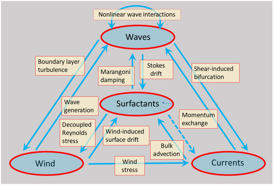
Figure 49.
Mechanisms whereby surfactants couple to the main dynamical processes that govern the ocean surface environment.
With regards to damping, the presence of a viscous cover and the Marangoni mechanism acts primarily on the shortest waves. The efficacy of nonlinear wave–wave interactions is not appreciably degraded by the oil film, so the quartic interactions drain wave energy from the lower wavenumber parts of the spectrum, near the spectral peak, to replenish the depleted spectral components at higher wavenumbers. This takes place on longer spatial and temporal scales than the Marangoni damping but, for sufficiently large patches, of the order of several kilometres, the resulting changes to the HF radar signature are predicted to be detectable. To put this in volumetric terms, an oil patch 10 km × 1 km with a thickness of 10 microns (giving the typical red to turquoise colour) requires less than 100 tonnes of oil. A large oil tanker may carry over 2 million barrels, i.e., 345,000 tonnes. We do not discount the possibility of a secondary role for skywave radar in detecting oil films, but we prefer to emphasise the ability of HF skywave radars to track Lagrangian surface drift currents, thereby supporting the prediction of oil spill movements and supporting the deployment of clean-up measures.
5. Conclusions
HF skywave radar combines four virtues that enable it to contribute to many different commercial, social, and scientific activities. First, it has vast coverage, extending to oceanic scales and matched only by spaceborne sensors. Second, and unlike the latter, it can provide persistent surveillance, so any important event or activity can be studied at a high resolution simultaneously in both space and time. Third, and most intriguingly, the scattering mechanisms that govern HF radio wave interaction with the geophysical environment yield characteristic signatures of a host of important phenomena. Fourth, a skywave radar is autonomous. If external factors intervene to close access to a service such as the WMO Information System (WIS), or block communications links to in situ sensors, other remote sensing technologies supplying societal needs may suffer catastrophic failure, but skywave radar is self-contained.
Our primary goal in this paper was to survey the prospective utility of modern skywave radars in a diverse range of societal activities, basing our survey on the 1974 NOAA report of Rhodes and Chadwick [101] but extending the spectrum of missions to include several critical tasks that have emerged in recent decades. Rather than explore the economic dimension, we have chosen to look more closely at the technical issues involved, taking care to delineate the limitations of the technology as well as its capabilities. We have optimistically assumed that our readership will include both (i) HF radar operators seeking new missions to address, and (ii) members of the maritime communities engaged in shipping, fishing, offshore oil and gas, and all the other topics treated in this paper. The amount of background material and the level of technical detail have been chosen to recognise this dichotomy.
The survey reveals that some of the contributions that skywave radar can make have no counterpart in other sensor technologies, and even where alternatives exist, they generally lack the same operational flexibility. It seems clear that the prospective benefits to shipping outweigh those for the other missions considered, largely because of the enormous volume of sea trade, where a small percentage gain in efficiency equates to a vast saving in costs. Nevertheless, almost all the missions we have examined possess some aspect that is best achieved with HF skywave radar, so having access to such a radar would be a strong motivation to employ it for these purposes.
The cost and complexity of the major skywave radars presently in operation might seem to render the prospective societal contributions of marginal relevance to the wider community but advances in microelectronics and computing power suggest that HF skywave radar need not be the preserve of the rich and powerful. Perhaps the most important ingredient is real estate.
It is our understanding that very few skywave radars presently take full advantage of their capabilities as multi-mission sensors, able to provide valuable support to a diverse range of human activities. As the primary role of all the radars shown in Figure 27 is national defence in the narrow interpretation, this is perhaps understandable, but we can hope that our survey will encourage these facilities to broaden their definition of defence and expand their clientele.
Funding
This research received no external funding.
Conflicts of Interest
The author declares no conflict of interest.
References
- Barrick, D.E. Remote sensing of sea state by radar. In Remote Sensing of the Troposphere; Derr, V.E., Ed.; NOAA/Environmental Research Laboratories: Boulder, CO, USA, 1972; pp. 12.1–12.6. [Google Scholar]
- Long, A.E.; Trizna, D.E. Measurements and Preliminary Interpretation of HF Radar Doppler Spectra from the Sea Echo of an Atlantic Storm; NRL Report 7456; Naval Research Laboratory: Washington, DC, USA, 1972. [Google Scholar]
- Long, A.E.; Trizna, D.B. Mapping of North Atlantic winds by HF radar sea backscatter interpretation. IEEE Trans. Antennas Propag. 1973, AP-21, 680–685. [Google Scholar] [CrossRef]
- Anderson, S.J. Over-the Horizon Radar Meteorology; Weapons Research Establishment Technical Report WRE-TR-1752 (A); Defence Science and Technology Group: Adelaide, Australia, 1977. [Google Scholar]
- Washburn, T.W.; Sweeney, L.E.; Barnum, J.R.; Zavoli, W.B. Development of HF skywave radar for remote sensing applications. In AGARD Special Topics in HF Propagation; SEE N80-19372 10-32; Advisory Group for Aerospace Research and Development: Neuilly-Sur-Seine, France, 1979. [Google Scholar]
- Anderson, S.J. Bistatic and Stereoscopic Configurations for HF Radar. Remote Sens. 2020, 12, 689. [Google Scholar] [CrossRef]
- Croft, T.A. Sky-Wave Backscatter: A Means for Observing our Environment at Great Distances. Rev. Geophys. Space Phys. 1972, 10, 73–155. [Google Scholar] [CrossRef]
- CODAR. Available online: https://codar.com (accessed on 15 November 2022).
- Available online: https://apollo.nvu.vsc.edu/classes/remote/lecture_notes/satellite/history/tiros.html#:~:text=Satellites%20with%20meteorological%20instrumentation%20were,this%20satellite%20was%2079%20days (accessed on 12 November 2022).
- Shutler, J.D.; Quartly, G.D.; Donlon, C.J.; Sathyendranath, S.; Platt, T.; Chapron, B.; Johannessen, J.A.; Girard-Ardhuin, F.; Nightingale, P.D.; Woolf, D.K.; et al. Progress in satellite remote sensing for studying physical processes at the ocean surface and its borders with the atmosphere and sea ice. Prog. Phys. Geogr. 2016, 40, 215–246. [Google Scholar] [CrossRef]
- Georges, T.M.; Maresca, J.W., Jr. Report on the Skywave Sea-State-Radar Workshop Held in Rockville, Maryland, 20–22 May 1981; NOAA Technical Memorandum ERL WPL-81; NOAA: Washington, DC, USA, 1981. [Google Scholar]
- Georges, T.M.; Maresca, J.W., Jr. Opportunities for New Ocean-Remote-Sensing Services Using Skywave Radar. In Proceedings of the IEEE Digest for 1981 International Geoscience and Remote Sensing Symposium, Washington, DC, USA, 8–10 June 1981; pp. 1395–1400. [Google Scholar]
- Anderson, S.J. Remote sensing applications of HF skywave radar: The Australian experience. Turk. J. Electr. Eng. Comput. Sci. 2010, 18, 339–372. [Google Scholar] [CrossRef]
- Headrick, J.M.; Anderson, S.J. HF Over-the-Horizon Radar. In Radar Handbook, 3rd ed.; Chapter 20; Merrill Skolnik; McGraw-Hill: New York, NY, USA, 2008. [Google Scholar]
- Anderson, S.J. Limitations to the extraction of information from multihop skywave radar signals. In Proceedings of the IEEE International Conference on Radar, Adelaide, Australia, 3–5 September 2003. [Google Scholar]
- Anderson, S.J. The Doppler structure of diffusely-scattered multi-hop skywave radar echoes. In Proceedings of the IEEE International Conference on Radar, Toulouse, France, 10–23 October 2004. [Google Scholar]
- Walsh, J.; Gill, E. An analysis of the scattering of high-frequency electromagnetic radiation from rough surfaces with application to pulse radar operating in backscatter mode. Radio Sci. 2000, 35, 1337–1359. [Google Scholar] [CrossRef]
- Anderson, S.J. Multiple scattering of HF surface waves: Implications for radar design and sea clutter interpretation. IET Radar Sonar Navig. 2010, 4, 195–208. [Google Scholar] [CrossRef]
- Anderson, S.J. Estimation and removal of multiple scattering contributions to HF surface wave radar echoes. In Proceedings of the IET Radar Conference, Hangzhou, China, 14–16 October 2015. [Google Scholar]
- Anderson, S.J. The Challenge of Signal Processing for HF Over-the-Horizon Radar. In Proceedings of the Workshop on Signal Processing and Applications, WOSPA’93, Queensland University of Technology, Brisbane, Australia, 13–15 December 1993. [Google Scholar]
- Anderson, S.J. OTH Radar Phenomenology: Signal Interpretation and Target Characterization at HF. IEEE Aerosp. Electron Syst. Mag. 2017, 32, 4–16. [Google Scholar] [CrossRef]
- Abramovich, Y.I.; Gorokhov, A.Y.; Mikhaylyukov, V.N.; Malyavin, I.P. Exterior noise adaptive rejection for OTH radar implementations. In Proceedings of the ICASSP ’94, IEEE International Conference on Acoustics, Speech and Signal Processing, Adelaide, Australia, 19–22 April 1994; pp. 105–108. [Google Scholar]
- Abramovich, Y.I.; Anderson, S.J.; Gorokhov, A.Y.; Spencer, N.K. Stochastic constraints method in nonstationary hot clutter cancellation, Part I: Fundamentals and supervised training applications. IEEE Trans. Aerosp. Electron. Syst. 1998, 34, 1271–1292. [Google Scholar] [CrossRef]
- Abramovich, Y.I.; Anderson, S.J.; Spencer, N.K. Stochastic-constraints method in nonstationary hot clutter cancellation, Part II: Unsupervised training applications. IEEE Trans. Aerosp. Electron. Syst. 2000, 36, 132–149. [Google Scholar] [CrossRef]
- Abramovich, Y.I.; Anderson, S.J.; Gorokhov, A.Y.; Spencer, N.K. Stochastically constrained spatial and spatio-temporal adaptive processing for nonstationary hot-clutter cancellation; Chapter 17. In Applications of Space-Time Adaptive Processing; Klemm, R.K., Ed.; IEEE: New York, NY, USA, 2004; pp. 603–697. [Google Scholar]
- Jannsen, P.A.E.M. On some consequences of the canonical transformation in the Hamiltonian theory of water waves. J. Fluid Mech. 2009, 637, 1–44. [Google Scholar] [CrossRef]
- Anderson, S.J.; Anderson, W.C. Bistatic scattering from the ocean surface and its application to remote sensing of seastate. In Proceedings of the 1987 IEEE APS International Symposium, Blacksburg, VA, USA, 15–19 June 1987. [Google Scholar]
- Stewart, R.H.; Joy, J.W. HF radio measurements of surface currents. Deep-Sea Res. 1974, 21, 1039–1049. [Google Scholar] [CrossRef]
- Skop, R.A. An approximate dispersion relation for wave-current interactions. J. Waterw. Port Coast. Ocean Eng. 1987, 113, 187–195. [Google Scholar] [CrossRef]
- Kirby, J.T.; Chen, T.M. Surface waves on vertically sheared flows: Approximate dispersion relations. J. Geophys. Res. 1989, 94, 1013–1027. [Google Scholar] [CrossRef]
- Ha, E.C. Remote sensing of Ocean Surface Current and Current Shear by HF Backscatter Radar. Ph.D. Thesis, Stanford University, Stanford, CA, USA, 1979. Technical Report D415-1. [Google Scholar]
- Teague, C. Multifrequency HF radar observations of currents and current shears. J. Ocean. Eng. 1986, 11, 258–269. [Google Scholar] [CrossRef]
- Vesecky, J.F.; Teague, C.C.; Onstott, R.G.; Daida, J.M.; Hansen, P.M.; Fernandez, D.; Schnepf, N.; Fischer, K. Observations of near-surface ocean currents at varying depths using a new multifrequency HF radar. In Proceedings of the IEEE International Geoscience and Remote Sensing Symposium, Singapore, 3–8 August 1997. [Google Scholar]
- Broche, P.; de Maistre, J.C.; Forget, P. Mesure par radar decametrique coherent des courants superficiels engenders par le vent. Oceanol. Acta 1983, 6, 43–53. [Google Scholar]
- Anderson, S.J. The HF radar signatures of surface gravity wave spectra on shear flows. In Proceedings of the Australian Institute of Physics Congress, Adelaide, Australia, 11–16 December 2022. [Google Scholar]
- Kenyon, K.E. Stokes drift for random gravity waves. J. Geophys. Res. 1969, 74, 6991–6994. [Google Scholar] [CrossRef]
- Punzmann, H.; Francois, N.; Xia, H.; Falkovich, G.; Shats, M. Generation and reversal of surface flows by propagating waves. Nat. Phys. 2014, 10, 658. [Google Scholar] [CrossRef]
- Rohrs, J.; Christensen, K.H. Drift in the uppermost part of the ocean. Geophys. Res. Lett. 2015, 42, 10–349. [Google Scholar] [CrossRef]
- Ardhuin, F.; Marie, L.; Rascle, N.; Forget, P.; Roland, A. Observation and estimation of Lagrangian, Stokes and Eulerian Currents Induced by Wind and Waves at the Sea Surface. J. Phys. Oceanogr. 2009, 39, 2820–2838. [Google Scholar] [CrossRef]
- Bye, J.A.T.; Wolff, J.-O.; Lettmann, K.A. A note on ocean surface drift with applications to surface velocities measured with HF radar. J. Oceanogr. 2017, 73, 491–502. [Google Scholar] [CrossRef]
- Van den Bremer, T.S.; Breivik, Ø. Stokes Drift. Philos. Trans. R. Soc. 2017, A376, 20170104. [Google Scholar] [CrossRef] [PubMed]
- Van der Mheen, M.; Pattiaratchi, C.; Cosoli, S.; Wandres, M. Depth-dependent Correction for Wind-driven Drift Current in Particle Tracking Applications. Front. Mar. Sci. 2020, 7, 305. [Google Scholar] [CrossRef]
- Tamtare, T.; Dumont, D.; Chavanne, C. The Stokes drift in ocean surface drift prediction. J. Oper. Oceanogr. 2021, 15, 156–168. [Google Scholar] [CrossRef]
- Wright, J.W. The wind drift and wave breaking. J. Phys. Oceanogr. 1976, 6, 402–405. [Google Scholar] [CrossRef]
- Lipa, B.; Nyden, B.; Barrick, D.E.; Kohut, J. HF radar sea-echo from shallow water. Sensors 2008, 8, 4611–4635. [Google Scholar] [CrossRef] [PubMed]
- Anderson, S.J. Symbiosis of remote sensing and ocean surveillance missions of HF skywave radar. In Ocean Remote Sensing Technologies: High Frequency, Marine and GNSS-Based Radar; Huang, W., Gill, E.W., Eds.; SciTech Publishing: London, UK, 2022. [Google Scholar]
- Anderson, S.J. Channel characterization for polarimetric HF skywave radar. In Proceedings of the IEEE Radar Conference, Washington, DC, USA, 2–6 May 2016. [Google Scholar] [CrossRef]
- Anderson, S.J. Prospects for tsunami detection and characterisation with HF skywave radar. In Proceedings of the 2008 International Conference on Radar, Adelaide, Australia, 2–5 September 2008; pp. 639–645. [Google Scholar] [CrossRef]
- Anderson, S.J. HF skywave radar performance in the tsunami detection and measurement role. In The Tsunami Threat—Research and Technology; Morner, N.-A., Ed.; IntechOpen: London, UK, 2011. [Google Scholar] [CrossRef]
- Occhipinti, G.; Dorey, P.; Farges, T.; Lognonné, P. Nostradamus: The radar that wanted to be a seismometer. Geophys. Res. Lett. 2010, 37, L18104. [Google Scholar] [CrossRef]
- Coisson, P.; Occhipinti, G.; Lognonne, P.; Molinie, J.-P.; Rolland, L.M. Tsunami signature in the ionosphere: A simulation of OTH radar observations. Radio Sci. 2011, 46, RS0D20. [Google Scholar] [CrossRef]
- Lipa, B. Derivation of directional ocean-wave spectra by integral inversion of second-order radar echoes. Radio Sci. 1977, 12, 425–434. [Google Scholar] [CrossRef]
- Trizna, D.B.; Headrick, J.M.; Bogle, R.W.; Moore, J.C. Directional sea spectrum determination using HF Doppler radar techniques. IEEE Trans. Antennas Propag. 1977, AP-25, 4–11. [Google Scholar] [CrossRef]
- Lipa, B. Inversion of second-order radar echoes from the sea. J. Geophys. Res. Ocean. 1978, 83, 959–962. [Google Scholar] [CrossRef]
- Anderson, S.J. The Extraction of Wind and Sea State Parameters from HF Skywave Radar Echoes; IREECON-83; IREECON International Digest: Sydney, Australia, 1983; pp. 654–656. [Google Scholar]
- Wyatt, L.R. A relaxation method for integral inversion applied to HF radar measurement of the ocean wave directional spectrum. Int. J. Remote Sens. 1990, 11, 1481–1494. [Google Scholar] [CrossRef]
- Howell, R.; Walsh, J. Measurement of ocean wave spectra using narrow beam HF radar. IEEE J. Ocean. Eng. 1993, 18, 296–305. [Google Scholar] [CrossRef]
- Hisaki, Y. Nonlinear inversion of the integral equation to estimate ocean wave spectra from HF radar. Radio Sci. 1996, 31, 25–39. [Google Scholar] [CrossRef]
- Barrick, D.E. The ocean waveheight nondirectional spectrum from inversion of the HF sea-echo Doppler spectrum. Remote Sens. Environ. 1977, 6, 201–227. [Google Scholar] [CrossRef]
- Barrick, D.E. Extraction of wave parameters from measured HF radar sea-echo Doppler spectra. Radio Sci. 1980, 12, 415–424. [Google Scholar] [CrossRef]
- Maresca, J.W.; Georges, T.M. Measuring rms waveheight and the scalar ocean wave spectrum with HF skywave radar. J. Geophys. Res. 1980, C-85, 2759–2771. [Google Scholar] [CrossRef]
- Barrick, D.E. Status of HF radars for wave-height directional spectral measurements. In Proceedings of the Symposium and Workshop on Wave-Measurement Technology, Washington, DC, USA, 22–24 April 1981; National Academy Press: Washington DC, USA, 1982; pp. 112–117. [Google Scholar]
- Weber, B.L.; Barrick, D.E. On the nonlinear theory for gravity waves on the ocean’s surface. Part I: Derivations. J. Physical. Oceanogr. 1977, 7, 3–10. [Google Scholar] [CrossRef]
- Barrick, D.E.; Weber, B.L. On the nonlinear theory for gravity waves on the ocean’s surface. Part II: Interpretation and applications. J. Phys. Oceanogr. 1977, 7, 11–21. [Google Scholar] [CrossRef]
- Creamer, D.B.; Henyey, F.; Schult, R.; Wright, J. Improved linear representation of ocean surface waves. J. Fluid Mech. 1989, 205, 135–161. [Google Scholar] [CrossRef]
- Wright, J.; Creamer, D.B. Improved linear representation of surface waves. Part 2. Slowly varying bottoms and currents. J. Fluid Mech. 1994, 261, 65–74. [Google Scholar] [CrossRef]
- Mao, Y.; Heron, M.L. The influence of fetch on the response of surface currents to wind studied by HF ocean surface radar. J. Phys. Oceanogr. 2008, 38, 1107–1121. [Google Scholar] [CrossRef][Green Version]
- Anderson, S.J.; Mahoney, A.R.; Zollo, A.O. Applications of Higher-Order Statistical Signal Processing to Radar, Chapter 13. In Higher-Order Statistical Signal Processing; Boashash, B., Powers, E.J., Zoubir, A.M., Eds.; Longman Australia and Halstead Press: Sydney, Australia, 1995; pp. 405–446. [Google Scholar]
- Anderson, S.J.; Mahoney, A.R.; Zollo, A.O. Diagnosis of Corrupted Skywave Radar Signals using Higher-Order Spectrum Analysis. In Proceedings of the IEEE International Conference on Acoustics, Speech and Signal Processing, ICASSP’93, Minneapolis, MN, USA, 27–30 April 1993. [Google Scholar]
- Jannsen, P.A.E.M. The Wave Model: May 1995. ECMRF Meteorological Training Course Lecture Series. 2003. Available online: https://www.ecmwf.int/sites/default/files/elibrary/2002/16951-wave-model.pdf (accessed on 2 September 2022).
- Anderson, S.J.; Abramovich, Y.I.; Skinner, A.I. Robust mapping of tropical cyclone wave fields using HF skywave radar. In Proceedings of the IEE Conference Publication 490, Proceedings of RADAR 2002, Edinburgh, UK, 15–17 October 2002; pp. 47–50. [Google Scholar]
- Stewart, R.H.; Barnum, J.R. Radio measurements of ocean winds at long ranges: An evaluation. Radio Sci. 1975, 10, 853–857. [Google Scholar] [CrossRef]
- Maresca, J.W., Jr.; Barnum, J.R. Measurement of oceanic wind speed from HF sea scatter by skywave radar. IEEE Trans. Antennas Propag. 1977, AP-25, 132–136. [Google Scholar] [CrossRef]
- Barnum, J.R.; Maresca, J.W.; Serebreny, S.M. High-resolution mapping of oceanic wind fields with skywave radar. IEEE Trans. Antennas Propag. 1977, 2, 128–132. [Google Scholar] [CrossRef]
- Parent, J.; Gaffard, C. Detection of meteorological fronts over the North Sea with Valensole skywave radar. IEEE J. Ocean. Eng. 1986, OE-11, 174–179. [Google Scholar] [CrossRef]
- Keenan, T.D.; Anderson, S.J. Some examples of surface wind field analysis based on JINDALEE skywave radar data. Aust. Meteorol. Mag. 1987, 35, 153–161. [Google Scholar]
- Young, G.S.; Harlan, J.A.; Georges, T.M. Application of over-the-horizon radar observations to synoptic and mesoanalysis over the Atlantic. Weather Forecast. 1997, 12, 44–55. [Google Scholar] [CrossRef]
- Anderson, S.J. On the sensitivity of HFSWR wave height and directional wave spectrum estimation to non-stationarity of forcing winds. In Proceedings of the IUGG General Assembly, IAPSO Session, Melbourne, Australia, 2 July 2011. [Google Scholar]
- Georges, T.M.; Harlan, J.A.; Leben, R.; Lematta, R.A. A test of ocean surface current mapping with over-the-horizon radar. IEEE Trans. Geosci. Remote Sens. 1998, 36, 101–110. [Google Scholar] [CrossRef]
- Trizna, D.B. Mapping ocean currents using over-the-horizon radar. Int. J. Remote Sens. 1982, 3, 295–309. [Google Scholar] [CrossRef]
- Georges, T.M.; Harlan, J.A. The first large-scale map of ocean surface currents made with dual over-the-horizon radars. In Proceedings of the OCEANS 96, MTS/IEEE Conference, Fort Lauderdale, FL, USA, 23–26 September 1996. [Google Scholar] [CrossRef]
- Georges, T.M.; Harlan, J.A.; Lee, T.N.; Leben, R. Observations of the Florida Current with two over-the-horizon radars. Radio Sci. 1998, 33, 1227–1240. [Google Scholar] [CrossRef]
- Anderson, S.J.; Buchan, S. HF radar detection of internal waves in the ocean. In Proceedings of the IEEE International Radar Conference, Lille, France, 13–17 October 2014. [Google Scholar]
- Anderson, S.J. HF radar signatures of ocean surface geometry and dynamics arising from localized disturbances. In Proceedings of the 2015 IEEE US Radar Conference, Arlington, VI, USA, 10–15 May 2015. [Google Scholar]
- Anderson, S.J. Monitoring the marginal ice zone with HF radar. In Proceedings of the IEEE US International Radar Conference, Seattle, WA, USA, 8–12 May 2017. [Google Scholar]
- Anderson, S.J. Remote Sensing of the Polar Ice Zones with HF Radar. Remote Sens. 2021, 13, 4398. [Google Scholar] [CrossRef]
- Anderson, S.J. HF radar signatures of rain-modified ocean surfaces. In Proceedings of the Asia-Pacific Microwave Conference, Adelaide, Australia, 11–13 August 1992. [Google Scholar]
- Anderson, S.J. Rainfall Detection. U.S. Patent 5,438,334, 1 August 1995. [Google Scholar]
- Anderson, S.J. Sensitivity of HF Radar Signatures of Ship Wakes to Hull Geometry Parameters. In Proceedings of the 21st Australasian Fluid Mechanics Conference, Adelaide, Australia, 10 December 2018. [Google Scholar]
- Anderson, S.J. HF radar signatures of ship and submarine wakes. J. Eng. 2019, 21, 7512–7520. [Google Scholar] [CrossRef]
- Anderson, S.J. HF Radar Scattering from a Sea Surface Perturbed by Multiple Ship Wakes. In Proceedings of the 2019 International Conference on Electromagnetics in Advanced Applications (ICEAA), Granada, Spain, 9–13 September 2019; pp. 0087–0089. [Google Scholar] [CrossRef]
- Anderson, S.J. Prospects for submarine detection with HF over-the-horizon radar. In Proceedings of the 6th Submarine Science, Technology and Engineering Conference, Adelaide, Australia, 8–10 November 2021. [Google Scholar]
- Anderson, S.J. HF radar detection and tracking of oil spills in the marine environment. In Proceedings of the IEEE International Geophysics and Remote Sensing Symposium, IGARSS’97, Singapore, 3 August 1997. [Google Scholar]
- Parent, J.; Bourdillon, A. Enhancement of remote sensing capability of HF skywave radar by correcting the signal for frequency modulations. In Proceedings of the Fourth International Conference on HF Radio Systems and Techniques, London, UK, 11–14 April 1988. [Google Scholar]
- Parent, J.; Bourdillon, A. A method to correct HF skywave backscattered signals for ionospheric frequency modulation. IEEE Trans. Antennas Propag. 1988, 36, 127–135. [Google Scholar] [CrossRef]
- Bourdillon, A.; Delloue, J.; Parent, J. Effects of geomagnetic pulsations on the Doppler shift of HF backscatter radar echoes. Radio Sci. 1989, 24, 183–195. [Google Scholar] [CrossRef]
- Anderson, S.J.; Abramovich, Y.I. A unified approach to detection, classification and correction of ionospheric distortion in HF skywave radar systems. Radio Sci. 1998, 33, 1055–1067. [Google Scholar] [CrossRef]
- Anderson, S.J. Adaptive Remote Sensing with HF Skywave Radar. IEE Proc. F 1992, 139, 182–192. [Google Scholar] [CrossRef]
- Anderson, S.J. Oceanographic and Meteorological Data. U.S. Patent 5,469,168, 21 November 1995. [Google Scholar]
- Earl, G.F.; Ward, B.D. The frequency management system of the Jindalee over-the-horizon backscatter HF radar. Radio Sci. 1987, 22, 275–291. [Google Scholar] [CrossRef]
- Rhodes, R.S.; Chadwick, R.B. Economic Appraisal of Real-Time Synoptic Sea-State Measurements by Over-the-Horizon Radar; NOAA Technical Report EREL 299-WPL 32; Environmental Research Laboratories: Boulder, CO, USA, 1974. [Google Scholar]
- Anderson, S.J. Remote sensing with the JINDALEE skywave radar. IEEE J. Ocean Eng. 1986, OE-11, 158–163. [Google Scholar] [CrossRef]
- Keenan, T.D.; Parker, P.R. National Significance of Meteorological Data Derived from the Jindalee Operational Radar Network; Working Paper; Australian Bureau of Meteorology Research Centre, Australian Government Bureau of Meteorology: Melbourne, Australia, 1992. [Google Scholar]
- Greenwald, R.A. History of the Super Dual Auroral Radar Network (SuperDARN)-I: Pre-SuperDARN developments in high frequency radar technology for ionospheric research and selected scientific results. Hist. Geo-Space Sci. 2021, 12, 77–93. [Google Scholar] [CrossRef]
- Baker, J.B.H. The Super Dual Auroral Radar Network (SuperDARN). Available online: http://vt.superdarn.org/tiki-index.php?page=sd_tutorial (accessed on 25 October 2021).
- Greenwood, R.; Schultz, E.; Parkinson, M.; Neudegg, D. Evaluation of the TIGER SuperDARN Over-The-Horizon Radar Systems for Providing Remotely Sensed Marine and Oceanographic Data Over the Southern Ocean; Technical Report No. 045; Australian Government, Bureau of Meteorology, Centre for Australian Weather and Climate Research: Melbourne, VIC, Australia, 2011. [Google Scholar]
- Available online: https://www.marinetraffic.com/en/ais/home/ (accessed on 12 November 2022).
- Available online: https://public.wmo.int/en/our-mandate/what-we-do/observations (accessed on 12 November 2022).
- Interim Report of Committee on Large Container Ship Safety; Ministry of Land, Infrastructure, Transport and Tourism, Government of Japan: Tokyo, Japan, December 2013.
- Young, I.; Babanin, A.V.; Zieger, S. The decay rate of ocean swell observed by altimeter. J. Phys. Oceanogr. 2013, 43, 2322–2333. [Google Scholar] [CrossRef]
- Lucas, C.; Soares, C.G. On the modelling of swell spectra. Ocean Eng. 2015, 108, 749–759. [Google Scholar] [CrossRef]
- Lipa, B.J.; Barrick, D.E.; Maresca, J.W. HF radar measurements of long ocean waves. J. Geophys. Res. 1981, 86, 4089–4102. [Google Scholar] [CrossRef]
- Available online: https://www.bloomberg.com/news/articles/2021-04-26/shipping-containers-plunge-overboard-as-supply-race-raises-risks (accessed on 12 November 2022).
- Bloomberg, L.P. Huge Spike in Shipping Containers Lost at Sea. Available online: https://gcaptain.com/shipping-containers-lost-at-sea/ (accessed on 1 January 2022).
- Ocean Container Losses Topple Annual Average in 2 Months. American Shipper. Available online: https://www.freightwaves.com/news/ocean-container-losses-topple-annual-average-in-2-months (accessed on 12 November 2022).
- Blenkey, N. IMO Moves on Container Losses at Sea. Marine Log, May 18, 2021. Available online: https://www.marinelog.com/legal-safety/safety-and-security/imo-moves-on-container-losses-at-sea/ (accessed on 12 November 2022).
- Anderson, S.J. A novel technique for measuring the surface wave Green’s function in the open sea, with applications to HFSWR. In Proceedings of the URSI General Assembly, Rome, Italy, 24 August–4 September 2021. [Google Scholar]
- Rousseau, Y.; Watson, R.A.; Blanchard, J.L.; Fulton, E.A. Evolution of global fishing fleets and the response of fished resources. Proc. Natl. Acad. Sci. USA 2018, 116, 12238–12243. [Google Scholar] [CrossRef]
- Morris, M.Y.; Roemmich, D.H.; Mayers, G.; Weisberg, R. Upper ocean heat and freshwater advection in the western Pacific Ocean. J. Geophys. Res. 1998, 103, 13023–13039. [Google Scholar] [CrossRef][Green Version]
- Figure Courtesy of Dr David Griffin, CSIRO, Australia. Data Was Sourced from Australia’s Integrated Marine Observing System (IMOS)—IMOS Is Enabled by the National Collaborative Research Infrastructure Strategy (NCRIS). It Is Operated by a Consortium of Institutions as an Unincorporated Joint Venture, with the University of Tasmania as Lead Agent. Available online: https://www.education.gov.au/ncris (accessed on 12 November 2022).
- Bagaglini, L.; Falco, P.; Zambianchi, E. Eddy detection in HF radar-derived surface currents in the Gulf of Naples. Remote Sens. 2019, 12, 97. [Google Scholar] [CrossRef]
- Roarty, H.; Cook, T.; Hazard, L.; George, D.; Harlan, J.; Cosoli, S.; Wyatt, L.; Alvarez Fanjul, E.; Terrill, E.; Otero, M.; et al. The Global High Frequency Radar Network. Front. Mar. Sci. Front. Media 2019, 6, 164. [Google Scholar] [CrossRef]
- Anderson, S.J.; Darces, M.; Helier, M.; Payet, N. Accelerated convergence of genetic algorithms for application to real-time problems. In Proceedings of the 4th International Symposium on Inverse Problems, Design and Optimization, Albi, France, 26–28 June 2013. [Google Scholar]
- Available online: https://www.maritimemanual.com/types-of-fishing-vessels (accessed on 12 November 2022).
- Klocker, A.; Abernathey, R. Global patterns of mesoscale eddy properties and diffusivities. J. Phys. Oceanogr. 2014, 44, 1030–1046. [Google Scholar] [CrossRef]
- Chelton, D.B.; Schlax, M.G.; Samuelson, R.M. Global observations of nonlinear mesoscale eddies. Prog. Oceanogr. 2011, 91, 167–216. [Google Scholar] [CrossRef]
- Rohrs, J.; Christensen, H.K.; Vikebø, F.; Sundby, S.; Saetra, Ø.; Brostrom, G. Wave-induced transport and vertical mixing of pelagic eggs and larvae. Limnol. Oceanogr. 2014, 59, 1213–1227. [Google Scholar] [CrossRef]
- Williams, R.G. Ocean eddies and plankton blooms. Nat. Geosci. 2011, 4, 739–740. [Google Scholar] [CrossRef]
- Gode, O.R.; Samuelsen, A.; Macaulay, G.J.; Patel, R.; Hjollo, S.S.; Horne, J.; Kaartvedt, S.; Johannessen, J.A. Mesoscale eddies are oases for higher trophic marine life. PLoS ONE 2012, 7, e30161. [Google Scholar] [CrossRef] [PubMed]
- Penna, A.D.; Gaube, P. Mesoscale eddies structure mesopelagic communities. Front. Mar. Sci. 2020, 7, 454. [Google Scholar] [CrossRef]
- Schmid, M.S.; Cowen, R.K.; Robinson, K.; Luo, J.Y.; Briseno-Avena, C.; Sponaugle, S. Prey and predator overlap at the edge of a mesoscale eddy: Fine-scale, in-situ distributions to inform our understanding of oceanographic processes. Sci. Rep. 2020, 10, 921. [Google Scholar] [CrossRef]
- Chang, Y.-L.; Miyazawa, Y.; Béguer-Pon, M. The dynamical impact of mesoscale eddies on migration of Japanese eel larvae. PLoS ONE 2017, 12, e0172501. [Google Scholar] [CrossRef]
- Suthers, I. Cited in CSIROscope, 3 June 2015. Available online: https://blog.csiro.au/expedition-to-study-ocean-eddies/ (accessed on 12 November 2022).
- Wang, X.; Wang, H.; Liu, D.; Wang, W. The prediction of oceanic mesoscale eddy properties and propagation trajectories based on machine learning. Water 2020, 12, 2521. [Google Scholar] [CrossRef]
- Available online: https://globalfishingwatch.org/research/global-footprint-of-fisheries/ (accessed on 12 November 2022).
- Kurup, N.V.; Shi, S. Study of nonlinear internal waves and impact on offshore drilling units. In Proceedings of the ASME 30th International Conference on Ocean, Offshore and Arctic Engineering, Rotterdam, The Netherlands, 19–24 June 2011. [Google Scholar] [CrossRef]
- Hein, J.R.; Mizell, K.; Koschinsky, A.; Conrad, T.A. Deep-ocean mineral deposits as a source of critical metals for high- and green-technology applications: Comparison with land-based resources. Ore Geol. Rev. 2013, 51, 1–14. [Google Scholar] [CrossRef]
- Sharma, R. Approach towards Deep-Sea Mining: Current Status and Future Prospects. In Perspectives on Deep-Sea Mining; Sustainability, Technology, Environmental Policy and Management; Springer: Cham, Switzerland, 2022. [Google Scholar]
- Miller, K.A.; Thompson, K.F.; Johnston, P.; Santillo, D. An overviews of seabed mining including the current state of development, environmental impacts, and knowledge gaps. Front. Mar. Sci. 2018, 4, 418. [Google Scholar] [CrossRef]
- Sharma, R. (Ed.) Environmental Issues of Deep Sea Mining: Impacts, Consequences and Policy Perspectives; Springer: Cham, Switzerland, 2019; ISBN 978-3-030-12696-4 (eBook). [Google Scholar] [CrossRef]
- Fukushima, T.; Tsune, A.; Sugishima, H. Comprehensive Understanding of Seafloor Disturbance and Environmental Impact Scenarios. In Perspectives on Deep-Sea Mining; Sustainability, Technology, Environmental Policy and Management; Springer: Cham, Switzerland, 2020; pp. 313–337. [Google Scholar] [CrossRef]
- Available online: https://www.isa.org.jm/ (accessed on 12 November 2022).
- International Union for the Conservation of Nature, Deep-sea mining, Issues Brief May 2022. Available online: https://www.iucn.org/resources/issues-brief/deep-sea-mining (accessed on 18 September 2022).
- Hylton, W.S. History’s Largest Mining Operation Is About to Begin. The Atlantic, January–February 2020 Issue. Available online: https://www.theatlantic.com/magazine/archive/2020/01/20000-feet-under-the-sea/603040/ (accessed on 12 November 2022).
- Deep-sea Mining. US Govt. Accountability Office Science & Tech Spotlight, 15 December 2021, GAO-22-105507. Available online: https://www.gao.gov/products/gao-22-105507 (accessed on 3 February 2022).
- Helmons, R.; de Wit, L.; de Stigter, H.; Spearman, J. Dispersion of benthic plumes in deep-sea mining: What lessons can be learned from dredging? Front. Earth Sci. 2022, 10, 868701. [Google Scholar] [CrossRef]
- Marshall, W.F.; Barnum, J.R. Measurement of Sea Scatter and Buoy Tracks at Long Ranges by High-Resolution OTH-B Radar; Stanford Research Institute Technical Report 1; Stanford Research Institute: Stanford, CA, USA, 1975. [Google Scholar]
- Li, L.; Wu, X.; Yan, S.; Long, C.; Liu, B.; Shen, Z. Drifter trajectory tracking experiment and analysis with multi-frequency HFSWR in the East China Sea. Wuhan Univ. J. Nat. Sci. 2011, 16, 541–547. [Google Scholar] [CrossRef]
- Kumar, N.; Cahl, D.L.; Crosby, S.C.; Voulgaris, G. Bulk versus spectral wave parameters: Implications on Stokes drift estimates, regional wave modelling, and HF radars applications. J. Phys. Oceanogr. 2017, 47, 1413–1431. [Google Scholar] [CrossRef]
- Breivik, O.; Janssen, P.A.E.M.; Bidlot, J.-R. Approximate Stokes Drift Profiles in Deep Water; European Centre for Medium-Range Weather Forecasting Technical Memorandum 716; ECMWF: Reading, UK, 2013. [Google Scholar]
- Dagestad, K.-F.; Rohrs, J. Prediction of ocean surface trajectories using satellite derived vs. modeled ocean currents. Remote Sens. Environ. 2019, 223, 130–142. [Google Scholar] [CrossRef]
- Christensen, K.H.; Breivik, O.; Dagestad, K.-F.; Rohrs, J.; Ward, B. Short-term predictions of oceanic drift. Oceanography 2018, 31, 59–67. [Google Scholar] [CrossRef]
- Breivik, O.; Allen, A.A.; Maisondieu, C.; Olagnon, M. Advances in search and rescue at sea. Ocean Dyn. 2013, 63, 83–88. [Google Scholar] [CrossRef]
- Van Sebille, E.; Aliani, S.; Law, K.L.; Maximenko, N.; Alsina, J.M.; Bagaev, A.; Bergmann, M.; Chapron, B.; Chubarenko, I.; Cózar, A.; et al. The physical oceanography of the transport of floating marine debris. Environ. Res. Lett. 2020, 15, 023003. [Google Scholar] [CrossRef]
- Available online: https://www.nasa.gov/mission_pages/hurricanes/features/hurricane_brew.html (accessed on 12 November 2022).
- Maresca, J.W., Jr.; Carlson, C.T. Tracking and Monitoring Hurricanes by HF Skywave Radar Over the Gulf of Mexico; Technical Report 1, Contract F49620-76-C-0023; SRI International: Menlo Park, CA, USA, 1977. [Google Scholar]
- Anderson, S.J. The remote sensing of tropical meteorological and oceanographic phenomena by over-the-horizon radar. In Proceedings of the 1st International Conference on Tropical Cyclones, Perth, Australia, 24 December 1979. [Google Scholar]
- Maresca, J.W., Jr.; Carlson, C.T. Comment on "Longshore currents on the fringe of hurricane Anita" by Ned P. Smith. J. Geophys. Res. 1980, 85, 1640–1641. [Google Scholar] [CrossRef]
- Maresca, J.W.; Carlson, C.T. High-frequency skywave radar measurements of Hurricane Anita. Science 1989, 209, 1189–1196. [Google Scholar] [CrossRef] [PubMed]
- Georges, T.M.; Harlan, J.A.; Meyer, L.R.; Peer, R.G. Tracking Hurricane Claudette with the U.S. Air Force OTH-B Radar; NOAA Technical memorandum ERL WPL-219; NOAA: Washington, DC, USA, 1992. [Google Scholar]
- Anderson, S.J. (Physics Department, University of Adelaide, Adelaide 5005, Australia). Unpublished work. 2019. [Google Scholar]
- Possner, A.; Caldeira, K. Geophysical potential for wind energy over the open oceans. Proc. Natl. Acad. Sci. USA 2017, 114, 11338–11343. [Google Scholar] [CrossRef]
- Available online: https://www.visualcapitalist.com/map-visualizing-40-years-of-nautical-piracy/ (accessed on 12 November 2022).
- ITOPF. Oil Tanker Spill Statistics 2021. Available online: https://www.itopf.org/knowledge-resources/data-statistics/statistics/ (accessed on 12 November 2022).


Publisher’s Note: MDPI stays neutral with regard to jurisdictional claims in published maps and institutional affiliations. |
© 2022 by the author. Licensee MDPI, Basel, Switzerland. This article is an open access article distributed under the terms and conditions of the Creative Commons Attribution (CC BY) license (https://creativecommons.org/licenses/by/4.0/).