1. Introduction
The 2021 EU Strategy on Adaptation to Climate Change emphasizes the importance of ensuring that fresh water is available in a sustainable manner and that water use is sharply reduced [
1]. Smart, sustainable, and optimized water use requires transformational changes in all sectors. However, agriculture is a major consumer of water resources, mostly through the application of irrigation [
2]. Farming activities account for almost 70% of global water use; in Mediterranean regions, this percentage can be even higher. In this context, planning sustainable policies and implementing better-informed decisions in water resource management are urgent needs for irrigated agriculture.
Assessing water withdrawal for crop irrigation from the field to the regional scale is crucial for effectively planning the sustainable allocation of water resources in agriculture, as well as for designing sustainable irrigation systems. Hence, in Europe, EU regulation No 1303/2013, consistent with the Water Framework Directive (WFD, 2000/60/EC), requires the implementation of operative procedures for assessing irrigation water volumes as a prerequisite for the exploitation of structural and investment funds within the EU Common Agricultural Policy [
3,
4].
From an operative perspective, in the case of collective irrigation schemes, withdrawal water volumes can be estimated from the net irrigation requirements of crops under “standard” conditions, as defined by the FAO 56 paper [
5], accounting for actual crop development.
In recent decades, accurate estimates of irrigation water requirements were achieved by implementing procedures based on crop–water balance models derived from the Penman-Monteith equation [
6], which is based on crop evapotranspiration under standard conditions [
5].
Those procedures mainly require knowledge of: (i) weather—from a complete set of meteorological data, including air temperature, wind speed, pressure, solar radiation, and relative humidity, to a limited set of data, such as only air temperature or solar radiation for simplified approaches; (ii) crop biophysical variables, such as leaf area index (LAI) or canopy cover (CC); and (iii) soil hydraulic properties, e.g., the field capacity and wilting point of various soil layers down to the bottom of the root zone [
5,
7].
Crop biophysical variables may be derived from dynamic crop growth models (CGMs), which are able to describe the behavior of the crop by modeling the physiological mechanisms of crop growth using mechanistic equations with different degrees of complexity [
8]. Among the CGMs described in literature, the Land and Water Division of FAO developed an easy-to-use modeling tool which is freely available to users: the AquaCrop model [
9]. For herbaceous crops, the model simulates the canopy cover, biomass, soil water components, and irrigation requirements for a given set of conditions over the whole growing cycle and estimates the final harvestable yield [
10]. The data required as input are a reduced number of crop parameters that can easily be observed in the field, as well as soil properties and weather information.
With the extensive development of Earth observation (EO) systems in recent decades, advanced techniques—which are able to provide crop biophysical parameter estimates by employing remote sensing imagery from instruments on board satellites—have spread rapidly [
11,
12,
13,
14,
15,
16] and become a valid and recognized component of CGMs, especially over large areas and for estimating crop parameters across the growing season with suitable temporal and spatial resolutions [
8,
13]. Several studies have proposed integration techniques between CGMs and satellite-based estimates of crop parameters obtained using freely available data from operational satellites, such as the USGS Landsat-8 or Copernicus Sentinel-2 missions [
8,
17,
18]. In September 2021, a new satellite in the Landsat series, Landsat-9, was launched to replicate its predecessor, Landsat 8, albeit with enhanced spatial resolution and temporal coverage. Operational data collection from the instruments onboard Landsat-9 began at the end of 2021, making this technology irrelevant to the present study, for which the newest technology is based on Sentinel-2 data.
The newest Sentinel-2 mission of the ESA-Copernicus program comprises a constellation of two identical satellites (Sentinel-2 A and B) that reduces, under cloud-free conditions, the revisit time to about 2–3 days at mid-latitudes and increases the possibility of obtaining cloud-free observations in key phenological periods during the crop growing cycle [
8]. An interesting feature of Sentinel-2 imagery is its spatial resolution of about 10 m over a broad range of spectral bands. The improved spectral, spatial, and temporal resolutions of the instruments onboard satellites make their imagery useful for accurate estimates of crop parameters (e.g., LAI and CC) from the field to the regional scale.
Regarding weather information, reliable crop–water balance models require a complete set of meteorological data, including air temperature, wind speed, pressure, solar radiation, and relative humidity. Ground-based weather stations equipped with a complete set of sensors are the main and preferred source of weather data, although such stations are generally limited in number, even in developed countries. Moreover, the observed time series can suffer from considerable time gaps, and often, protocols for correcting and estimating poor quality or missing data must be used [
19].
Therefore, recent studies have focused on the possibility of employing reanalysis weather data as a gridded source for water resource management studies, since they represent a complete and consistent climate dataset that covers several decades with suitable spatial resolutions [
19,
20,
21,
22,
23,
24]. The results of these studies encouraged the use of reanalysis data as valuable proxy of ground weather observations for reference evapotranspiration from the local to the regional scale. Reference evapotranspiration is a key variable for studies on crop water requirements [
5].
In addition, more recent studies have investigated alternative sources of solar radiation data, i.e., from satellite-based products, showing that such data achieve better performance than reanalysis solar radiation outputs [
24,
25,
26]. One such study proposed an optimal blend of weather information between reanalysis and satellite-based solar radiation data for assessing reference evapotranspiration [
24].
Among satellite-derived solar radiation data, those based on sensors mounted on geostationary satellites, like the Meteosat Visible and Infrared Imager (MVIRI) onboard the ESA Meteosat First Generation and the Spinning Enhanced Visible and Infrared Imager (SEVIRI) on board the ESA Meteosat Second Generation satellites, are made freely available to users by different institutes that elaborate the raw data with their own algorithms. Among these, products from the Satellite Application Facility on Climate Monitoring (CM-SAF,
www.cmsaf.eu; accessed on 12 July 2021) are of very high quality [
24,
26,
27,
28].
In this study, we implemented a procedure based on the most advanced data for assessing crop water requirements by combining the AquaCrop model with crop input parameters estimated based on Sentinel-2 imagery during the crop growing cycle. In addition to using a complete set of ground-based weather data, we also evaluated the use of the weather reanalysis ERA5-Land database combined with satellite-based solar radiation data from CM-SAF. This is the first report of the implementation of such an approach in the literature.
The objectives of the study were: (i) to show the improvements in terms of predicted crop water requirements and yield if satellite-based crop parameter estimations were assimilated into the crop dynamics during the AquaCrop simulations; and (ii) to demonstrating that the merged ERA5-Land and CM-SAF database represents a reliable and accurate remote proxy of ground weather observations for the assessment of crop water requirements and yield if combined with satellite-based crop parameter estimates.
The benchmark scenario of the analysis was the AquaCrop simulation outputs when only a complete set of ground-based weather data was implemented as input information.
An evaluation of the proposed procedure is presented, using a farm located in Southern Italy, where a field campaign was conducted in the irrigation season of 2021 for the target crop, i.e., tomato. The field campaign supplied data for validating the satellite-based estimates of crop parameters (i.e., canopy cover) and setting input field and crop management data for the specific crop, as well as for validating the outputs of the procedure, both in terms of final yield and crop water requirements.
2. Materials and Methods
2.1. Study Area and Field Data
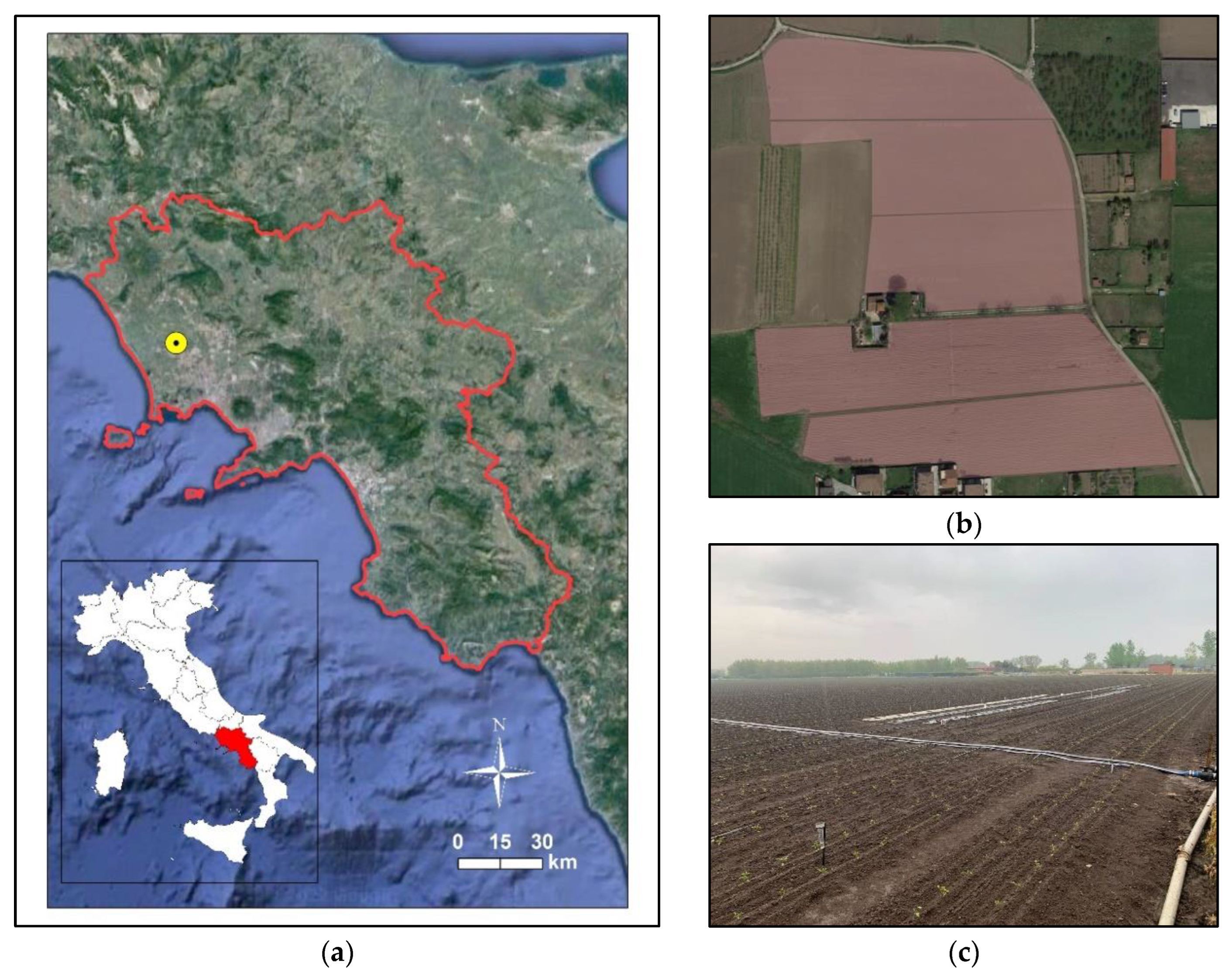
The study area was a farm of about nine hectares located in the Campania region, Southern Italy (
Figure 1). The climate of the region is classified as Mediterranean, under the Köppen-Geiger climate classification; it is characterized by hot and dry summers, warm springs, and mild and wet winters and autumns. During summer, the mean monthly temperature ranges from 25 to 30 °C. The annual precipitation ranges from 800 to 1100 mm. The maximum monthly precipitation values are recorded during November and December, while the minimum values occur during July and August.
Agriculture is one of the main economic activities in the region. Irrigation in open fields generally starts in April and lasts until July or September, according to the specific crops and agricultural practices.
The year of the present analysis was 2021, when a field campaign was conducted on the farm of interest. On the farm, a unique crop is cultivated on all 9 hectares, and crop alternation takes place. In 2021, the cultivated crop was processing tomato (Solanum Lycopersicum), cultivar Heinz 5108, which was chosen as the crop of interest for the present study. The crop was transplanted at the beginning on April 8 and harvested on July 20. Irrigation was performed using a drip irrigation system.
In the proximity of the farm, a ground-based automatic weather station (AWS) providing measurements of precipitation, atmospheric pressure, solar radiation, air relative humidity, wind speed at 10 m above ground level, and air temperature at 2 m, with high accuracy and precision standards, has been working since 2008 as part of the regional monitoring network managed by the Regional Hydrometeorological Service [
29].
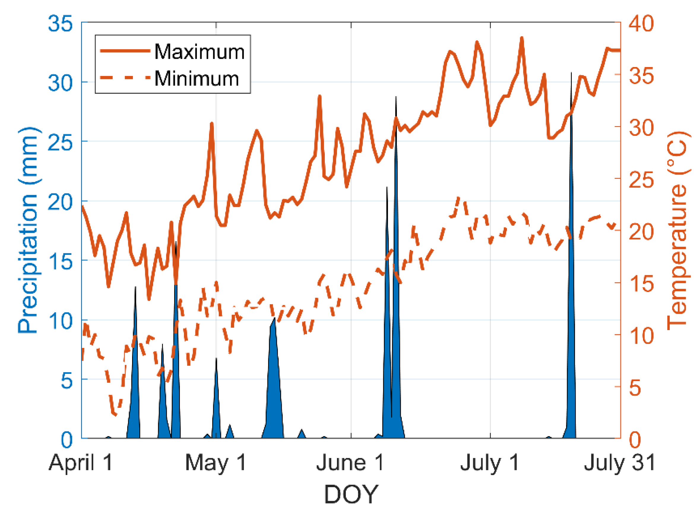
Total precipitation during the April–July 2021 season was about 165 mm; there were 18 rainy days. However, rainfall greater than 2 mm only occurred on 11 days.
Figure 2 shows daily precipitation and maximum and minimum temperatures from April 1 to July 31 in 2021.
Table 1 shows some statistics of the observed weather variables, computed at the location of the AWS in April–July of years 2008–2021.
Then, the data of the field campaign were used as either calibration or validation sets for the proposed procedure, as specified below, consisting of:
Field and crop management: date of sowing and harvesting, irrigation technique.
Irrigation schedule and volumes.
Canopy cover measurements.
Yield.
The dates of sowing and harvesting were used as calibration data for the AquaCrop model (
Section 2.5), along with the irrigation system and technique.
A drip irrigation system was available at the farm: plants were watered by light driplines, with 30 cm dripper spacing and 2 L/ha flow rate at 1 bar. Based on the farmer’s practices, plants were irrigated to ensure that the root zone (water) depletion (RZD) was always above 50% of the readily available water (RAW) [
30]. The cumulative irrigation amount given by the farmer was 294 mm (29.4 m
3/ha) throughout the whole growing period (9 April to 17 July).
Table 2 reports the days of irrigation chosen by the farmer according to both his expertise and field measurements of soil humidity. Each irrigation event was characterized by a constant amount of water of 14 mm. The total irrigation volume was considered as a reference value for evaluating the different estimation methods that were tested, as described below.
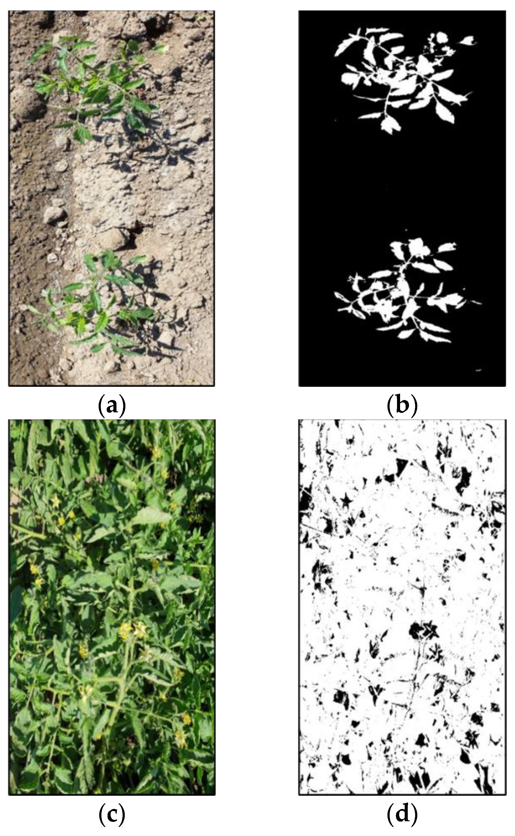
During the growing period, measurements of canopy cover were also taken. CC, generally expressed as a percentage, represents the extension of the canopy per unit of soil surface; it is is one of the key parameters for estimating crop evapotranspiration in agro-hydrological models, such as the AquaCrop model (
Section 2.5). The degree of canopy cover ranges from 0% (no green cover) to 100% (green cover). CC measurements were taken simultaneously to Sentinel-2 satellite acquisitions or within 5 days from the day of satellite imagery acquisition (
Section 2.2) using high-resolution pictures of the soil (
Figure 3a–c), taken with a 108 megapixel camera. The pictures were analyzed using the free software, Canopeo. Canopeo is a green vegetation image analysis tool that examines and classifies all the pixels in an image according to color scales defined by red-green-blue (RGB) combinations. The pixels in the image are classified according to the ratios of R/G, B/G [
31], and the excess green index [
32]. The result of the analysis is a binary image (
Figure 3b–d) in which white pixels correspond to those that satisfy the selection criteria (green cover) and black pixels correspond to those that do not (no green cover).
Since punctual field measurements of CC were used to validate the satellite-based estimates of CC (
Section 2.2) that have a spatial resolution of 20 m × 20 m, field data were collected following the Validation of Land European Remote-Sensing Instruments (VALERI) protocol [
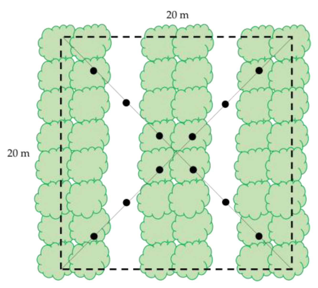
33]. The VALERI protocol provides a sampling strategy for the validation of high-spatial resolution satellite products by using elementary sampling units (ESUs) of 20 m × 20 m. For this study, with the aim of describing spatial CC variability, 10 ESUs were located in the crop field, assuming a minimum distance of 20 m from the edges of the field [
34].
For each ESU, 12 measurements were collected following square spatial sampling (
Figure 4). Then, the mean value of these measurements was assumed to be representative of each ESU and was used for the comparison with the corresponding satellite-based estimate of CC (the fractional vegetation cover products are described in
Section 2.2).
Table 3 reports the crop field mean, minimum, and maximum values of CC, along with the dates of acquisition.
Finally, the amount of yield was measured at the end of the season (at the harvesting date, 20 July); it was equal to 121 t/ha. This value was a key parameter for the validation of the following analyses.
2.2. Sentinel-2 Imagery for Crop Parameter Estimation
In this study, we exploited the full temporal and spectral capabilities of the Multispectral Instrument (MSI) sensor on board the Sentinel-2A (S2A) and Sentinel-2B (S2B) satellites of the ESA-Copernicus program. Thanks to the Sentinel-2 (S2) characteristics, outlined in
Table 4 [
35], it was possible to derive key information with which to monitor crop growth development.
During the growing season, the field campaigns coincided with the overpass dates of S2 over the study area, with a maximum difference of five days due to the cloud cover. The images were downloaded directly and free of charge from the THEIA Land Data Center [
36].
The THEIA data center provides S2 Level-2A (L2A) images, which are already geometrically and atmospherically corrected by means of the MACCS-ATCOR Joint Algorithm (MAJA) processor [
37]. The MAJA processor is an evolution of the Multi-sensor Atmospheric Correction and Cloud Screening (MACCS) [
38] integrated within the Atmospheric Correction (ATCOR) software [
39], that converts S2 Level-1C data (L1C—top of the atmosphere reflectance) into atmospherically corrected S2 images (L2A—surface reflectance), including adjacency effect (L2A SRE—Surface REflectance) and slope correction (L2A FRE—Flat REflectance) [
37].
In this study, 12 available cloud-free L2A FRE acquisitions over the study area from S2 were downloaded (
Table 5).
Subsequently, these images were resampled to 10 m pixel and processed in the SNAP toolbox to determine the Fractional Vegetation Cover (FVC) by using the Biophysical Variables Processor. This processor further computes the Level-2B (L2B) biophysical products, such as the Leaf Area Index (LAI), Canopy Chlorophyll content (CCC), Canopy Water Content (CWC), and the fraction of Absorbed Photosynthetically Active Radiation (fAPAR) variables, by using a Neural Network (NNET) trained with a globally representative set of simulations from a canopy Radiative Transfer Model (RTM), named PROSAIL [
40].
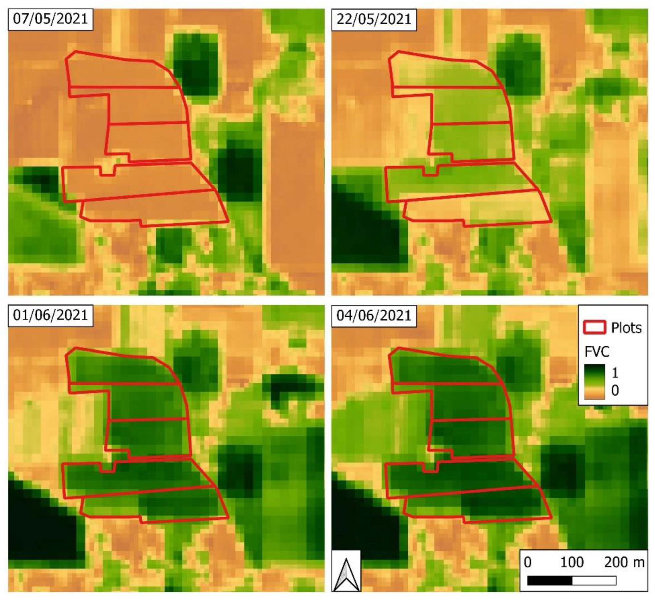
In this study, the FVC maps (
Figure 5) were computed using SNAP version 8.0, where the biophysical processor allows the selection of two specific NNET trained for S2A and S2B [
41]. During this process, for each considered acquisition, the FVC quality indicator maps were derived automatically with the aim of excluding invalid pixels, in accordance with [
40].
Figure 5 shows four of the FVC maps used in the present study.
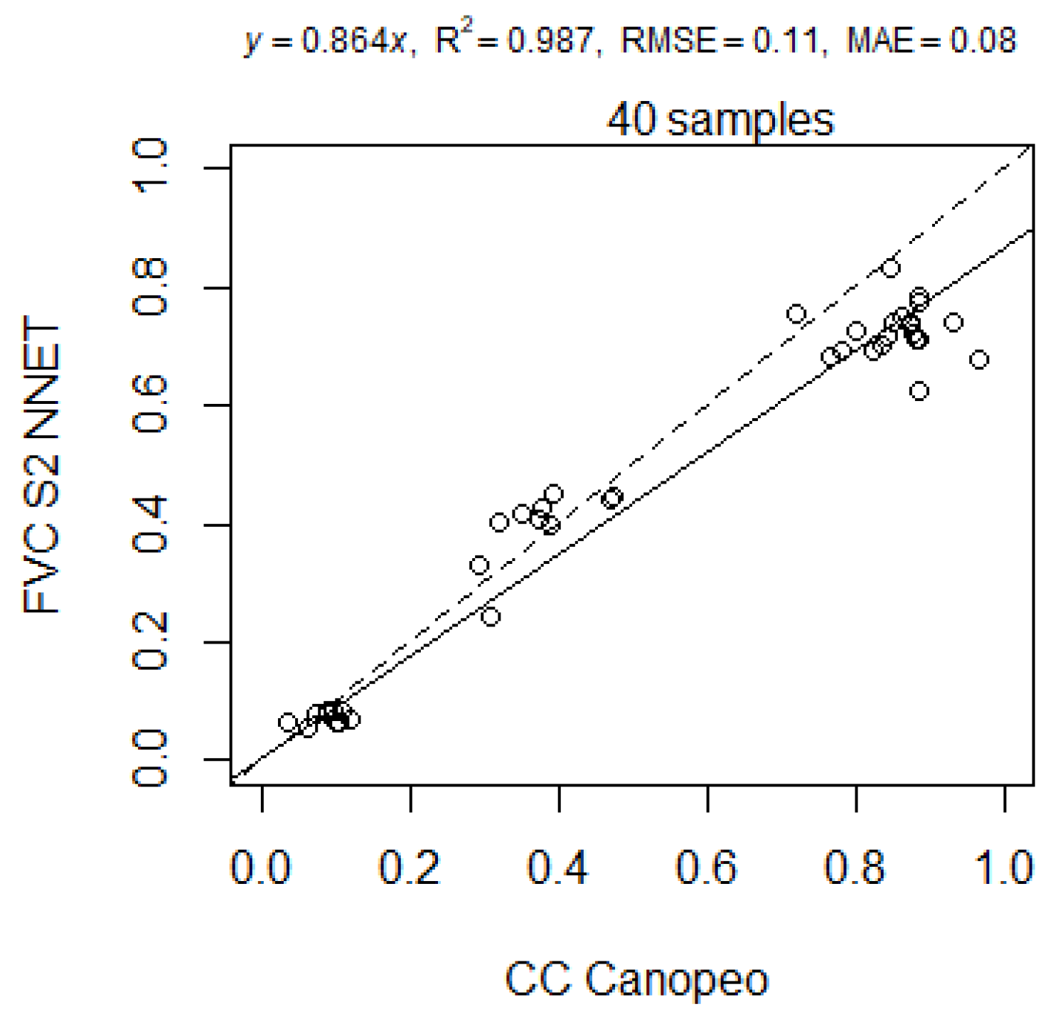
The S2 FVC is formally equivalent to the CC, so we assumed FVC to be a proxy of the ground measurements of CC. The soundness of this assumption was confirmed by comparing and validating the satellite-based FVC measurements with the field CC measurements acquired with the VALERI protocol (
Section 2.1).
Figure 6 shows the results of this comparison, which clearly support this assumption.
2.3. Meteorological Data: ERA5-Land Reanlysis and CM-SAF Satellite-Based Solar Radiation
The availability of consistent, long, and complete time series of meteorological data is a crucial aspect for the estimation of crop water requirements, since weather represents the most important input variable for assessing crop evapotranspiration that, in turn, determines the water deficit in soil (
Section 2.5). In recent years, meteorological reanalysis products have been used in many applications as gridded input data where a complete reconstruction of past weather was required [
4,
24,
42]. The use of reanalysis data has been motived, in many regions of the word, by the lack of dense ground-based measurements of weather variables that include all the variables needed for the estimation of the crop evapotranspiration, such as wind speed, air relative humidity, air pressure, and incoming solar radiation, as well as air temperature [
4,
24,
43]. Another motivation to use reanalysis data as a proxy of ground weather data is the increased reliability of the outputs of the most advanced numerical weather prediction models [
44,
45]. Indeed, reanalysis data are obtained by retroactively running those models with a sequential assimilation of the available land surface and atmospheric observations from across the world.
ERA5-Land (ERA5L) is the most advanced global reanalysis dataset produced in Europe, specifically conceived for land surface applications, and obtained using, as atmospheric forcing, the land fields of ERA5 atmospheric variables. ERA5 is the fifth and last generation of ECMWF global reanalysis [
46] with a spatial resolution of about 31 km. ERA5-Land data have a native horizontal resolution of about 9 km; data are in the form of a regular 0.1° × 0.1° grid, covering the period from 1981 to 2–3 months before the present. In this study, we assessed the ability of ERA5-Land data to serve as a proxy of ground-based observations in our analysis. Raw data are freely available on the website
https://cds.climate.copernicus.eu; accessed on 18 July 2020) [
47].
ERA5-Land data are produced with an hourly time-step. Thus, minimum, maximum, and mean daily values of weather variables were derived by gathering 24 values, starting from UTC+ 2 every day. The weather variables of interest were air temperature at 2 m, wind speed at 10 m, dew point temperature at 2 m, and barometric pressure. The daily mean dew point temperature was used to compute the daily mean of the actual vapor pressure, instead of air relative humidity, as done for the ground-based data [
5,
24].
In this study, ERA5L surface incoming solar radiation (Rs) was replaced with the Rs retrieved by the Satellite Applications Facility on Climate Monitoring (CM-SAF) from the instruments on board the Meteosat geostationary satellites. A recent study [
24] demonstrated that the use of a blended dataset of meteorological data, composed of ERA5L data and CM-SAF satellite-based solar radiation data, was a better choice for achieving reliable reference evapotranspiration estimates than a complete dataset of ERA5L products. The daily means of CM-SAF surface incoming shortwave radiation are provided via a web user interface on the CM-SAF website (
http://wui.cmsaf.eu; accessed on 12 July 2021) on a regular grid with a spatial resolution of 0.05° × 0.05°. The products are part of SARAH-2.1 [
48], which is a satellite-based climate database derived from the measurements taken by both Meteosat First Generation and Meteosat Second Generation satellite equipment, such as the Meteosat Visible and Infrared Imager (MVIRI) and the newest Spinning Enhanced Visible and Infrared Imager (SEVIRI). The CM-SAF algorithm is based on the evaluation of the interaction between the atmosphere, clear sky reflection, transmission, and the top of atmosphere albedo by implementing a radiative transfer model and a look-up table method [
49,
50]. Conversion from the irregular satellite projection to a regular 0.05° × 0.05° geographic grid is then performed with a gridding tool based on a nearest-neighbor method.
2.3.1. Downscaling and Bias Correction of Meteorological Data
The weather data comprising both ERA5L reanalysis and CM-SAF products are available as points of regular geographic grids with different resolutions. The method to transfer the information from those points to the sites of interest within the grid is called downscaling.
In this study, statistical downscaling techniques were employed to infer reanalysis and satellite-based data from the native grid to the site of interest. Then, downscaled data were bias corrected to remove the systematic errors from the estimates.
The downscaling of ERA5L data was performed by a triangle-based bi-linear interpolation method [
51] that consists of interpolating the three grid points closest to the examined site. For CM-SAF products, the nearest grid point was considered instead, since the satellite product is a pixel-integrated measurement of the parameter of interest.
The bias correction of data was performed by computing an average bias between reanalysis/satellite-based data and ground-based observations at the site and period of interest (April–July) in 2018–2020 for each of the weather variables. These biases were then subtracted from the reanalysis/satellite-based estimates for 2021. Similar ameliorative bias correction performance for numerical weather predictions was observed when different and more complex correction schemes were applied [
20,
52].
Here, as in previous studies [
4,
24], bias correction was applied when ground weather observations were not available in the year of interest but data from prior years (e.g., here, a triennium) were available for calibration.
2.4. FAO Penman-Monteith Reference Evapotranspiration
Reference evapotranspiration is a variable that depends entirely on meteorological data, since it is computed for a reference crop, under standard conditions; it represents the reference evaporative demand. This is the reason why it can be used as a good and concise indicator for assessing the performance of different weather databases, such as the merged ERA5-Land and CM-SAF database, compared to ground observations.
In this study, the daily reference evapotranspiration, ET
0 (mm day
−1), was computed with the FAO Penman–Monteith equation [
5] as follows:
where λ is the latent heat of vaporization, equal to 2.45 MJ kg
−1; Δ (kPa °C
−1) is the slope of the vapor pressure curve; γ is the psychometric constant (kPa °C
−1); T (°C) is the daily mean air temperature at a height of 2 m, computed as the average between the daily maximum (T
max) and minimum (T
min) air temperatures at the same height; WS (m s
−1) is the wind speed at a height of 2 m; e
s (kPa) and e
a(kPa) are, respectively, the daily saturation vapor pressure and daily actual vapor pressure, which are computed from the maximum and minimum temperatures and, alternatively, from air relative humidity or dew point temperature; Rn (MJ m
−2 day
−1) is the net radiation at the crop surface; and G (MJ m
−2 day
−1) is the soil heat flux density. The net radiation (Rn) was calculated as the difference between the incoming net shortwave radiation and the outgoing net long-wave radiation. The former is a fraction of the incoming shortwave solar radiation (Rs), computed for the reference crop by setting the albedo to 0.23. The daily mean wind speed at a height of 2 m, WS (m s
−1), was obtained from the wind speed at a height of 10 m using a logarithmic wind speed profile, as suggested by [
5]. More details about the parameters in Equation (1), omitted here for the sake of brevity, can be found in the FAO irrigation and drainage study No. 56 [
5].
2.5. AquaCrop Model for Crop Water Requirements and Yield Estimation
AquaCrop is a crop growth model developed by FAO’s Land and Water Division that simulates crop yield and water requirements with daily time increments [
53]. Although AquaCrop can reproduce the soil–water stress that may affect canopy expansion and transpiration, as well as biomass and final yield, in this study, we forced well-watered conditions by imposing irrigation when a chosen soil moisture threshold was reached (
Section 2.5.1).
The AquaCrop model can be briefly described through the following four stages of a simulation that takes into account the key variables of the process:
Crop development, which is expressed through green canopy cover (CC) and depends on the water content in the soil profile each day. Canopy development over time is modeled with a sigmoid function using a canopy growth coefficient (CGC). Senescence of the canopy is simulated with a decline function parametrized by a canopy decline coefficient (CDC), used to describe the declining phase due to leaf senescence as the crop approaches maturity [
54].
Evapotranspiration estimates, which are required for daily soil water balance and are achieved by dividing evapotranspiration into soil evaporation and crop transpiration. Soil evapotranspiration is assumed to be proportional to the area of soil not covered by vegetation, while crop transpiration (Tr) is calculated by multiplying the reference evapotranspiration (ET0) with a crop coefficient (Kc). The crop coefficient is proportional to CC and, hence, varies throughout the life cycle of the crop, in accordance with the simulated canopy cover. Reference evapotranspiration is determined by the FAO Penman–Monteith equation and depends on daily weather data.
Above-ground biomass (B) is assumed to be proportional to the cumulative amount of crop transpiration by a factor known as biomass water productivity (WP), here normalized for climate [
54]. WP expresses the aboveground dry matter produced per unit land area per unit of water transpired [
54].
Finally, crop yield (Y) is obtained from B using a harvest index (HI), which is the fraction of B that is harvestable product.
The model parameters may be grouped into two classes: conservative and non-conservative. Conservative parameters are not dependent on local and management conditions, such as the canopy growth (CGC) and canopy decline (CDC) coefficients, the full canopy crop transpiration coefficient (Kc), and the biomass WP and soil water depletion thresholds. Non-conservative parameters vary depending on crop and field management, soil type, and climate (sowing date and density, length of crop cycle and phenological stages, maximum canopy cover, etc.). These parameters can be either retrieved from the AquaCrop literature or calibrated by the user (e.g., by means of field experiments).
2.5.1. AquaCrop Implementation: Input, Calibration, and Validation Data
In this study, a limited number of AquaCrop parameters were calibrated with field information related to the crop management at the farm of interest. The data used for the calibration of the model were the transplant dates and densities, flowering date, and duration, starting of senescence, maturity, and date of harvesting.
To simulate irrigation, the model was set in net irrigation requirement mode, which estimates the crop water requirements based on a selected threshold of allowed root zone (water) depletion (RZD) to reproduce the irrigation method used at the farm of interest. The threshold of RZD was set at 50% of the readily available water (RAW), and drip irrigation was simulated by setting a constant amount of water for each irrigation event, i.e., 14 mm, as done by the farmer (
Table 2). The chosen threshold imposed well-watered conditions and no crop water-stress conditions.
The canopy cover (CC) is equivalent to the fractional vegetation cover (FVC) estimated by Sentinel-2 imagery. Hereafter, we use the two terms canopy cover (CC) and fractional cover (fc) to distinguish the two variables, respectively derived with AquaCrop and Sentinel-2 imagery (
Section 2.2). In this study, we corrected the estimates of CC by assimilating the satellite-based fractional cover as soon as a satellite acquisition was available.
Input data were also the weather data from two sources: ground-based meteorological stations (
Section 2.1) and the merged ERA5-Land and CM-SAF database (
Section 2.3).
The main AquaCrop outputs are crop production (biomass and yield) and crop water requirements. The data used to validate the results of the model were the total irrigation volume that the farmer chose according to his expertise and the final amount of yield that was effectively harvested (
Section 2.1).
2.5.2. Assimilation of Sentinel-2 FVC into AquaCrop
In this study, we corrected the temporal evolution of canopy cover given by the model by sequentially assimilating the satellite-based fractional cover as soon as new satellite data were available. The assimilation technique was basically a direct insertion of the satellite-based estimate of fractional cover (i.e., S2 FCV) in place of the canopy cover (CC) simulated by the model.
The sequential direct insertion was applied under the assumption that a continuous update of one crop model state based on remote observations would reduce the biases induced by the model simplifications of the processes and environmental conditions influencing the crop growth dynamics [
30].
2.6. Statistical Indices for Evaluating Performance
The performance indicators were selected based on commonly used indicators in analogous previous studies (e.g., [
22,
24,
25]):
The percent BIAS (PBIAS, %), which is used as an indicator of accuracy:
where P
i and O
i are, respectively, the variable for which the performance evaluation is desired and the corresponding observed variable at the ith day; n denotes the number of examined days; and
is the mean of the observations computed over the examined days. The more the PBIAS differs from zero, the less accurate the estimate; PBIAS < 0 suggests, on average, an underestimation, while PBIAS > 0 implies an overestimation.
Besides the PBIAS, the absolute BIAS, ABIAS, was also used as an indicator of both accuracy and precision. It was computed as follows:
The lower the value of ABIAS, the better the estimate.
Then, we used the percent root mean square error (PRMSE, %), which gives insights into both accuracy and precision; the greater the PRMSE, the less accurate and precise the estimates.
3. Results
The results of the present study were first presented in terms of the performance of the merged ERA5-Land and CM-SAF database compared to the ground observations for the assessment of temperature and reference evapotranspiration, that comprise the key forcing input data of the AquaCrop model (
Section 3.1). Indeed, one of the main working hypotheses to be validated in this study was that the merged ERA5-Land and CM-SAF database would, if assimilated with S2 FVC, represent a reliable and accurate remote proxy of ground weather observations for the assessment of crop water requirements and yield.
Another objective of this study concerned the possibility of using Sentinel-2 imagery to improve crop water requirements and yield estimations by assimilating S2 FVC into the canopy cover dynamics during the AquaCrop simulations if either ground weather observations or remote proxy of ground weather observations were available. The main results of the study regarding the outputs of the AquaCrop simulations are presented for three different scenarios that required different input datasets: (i) only weather ground observations; (ii) weather ground observations and S2 FVC; and (iii) the merged ERA5-Land and CM-SAF database and S2 FVC.
A comparison of scenarios (i) and (ii) supports the objective of the study related to the improvements of model outputs due to the assimilation of S2 FVC into the AquaCrop model, while a comparison of scenarios (ii) and (iii) shows that a remote proxy of ground weather observations can serve as a valid replacement for ground weather observations that may be not available at large scales.
The “best estimate” scenario is the second scenario, assumed as a comparative scenario below, since it regards the optimal option of availability of both weather observations and S2 FVC.
The results are provided for all the three scenarios in terms of canopy cover dynamics, crop evapotranspiration, recommended irrigation volumes (i.e., crop water requirements), and yield. Statistics, i.e., absolute BIAS (ABIAS), are given for scenario (i) and (iii) with regards to scenario (ii). Recommended irrigation volumes and yield were also compared to the available field data (
Section 2.1) to validate the hypotheses of this study.
3.1. Reference Evapotranspiration and Temperaure
Table 6 shows the performances of the ERA5L temperature and reference evapotranspiration computed from the merged ERA5-Land and CM-SAF database (ERA5L + CMSAF ET
0) for 2021 both before (raw data) and after bias correction (as described in
Section 2.3.1). The benchmarks for the computation of PBIAS and PRMSE are the ground observed temperature and reference evapotranspiration computed from ground observations at the site of interest by implementing Equation (1).
Here, the temperature is the daily mean air temperature at a height of 2 m, computed as the average between the daily maximum (Tmax) and minimum (Tmin) air temperatures at the same height.
The PBIAS of raw ERA5L temperature was reduced by 6.5% (with respect to zero) thanks to the bias correction, while the PRMSE was reduced by 5%. Regarding the ERA5L + CMSAF ET0, the PBIAS was reduced by 8.5%, while the PRMSE was reduced by 4.4%.
In the next sections, all the other results refer to the use of the bias corrected temperature and reference evapotranspiration.
3.2. Canopy Cover Dymanics and Crop Evapotranspiration
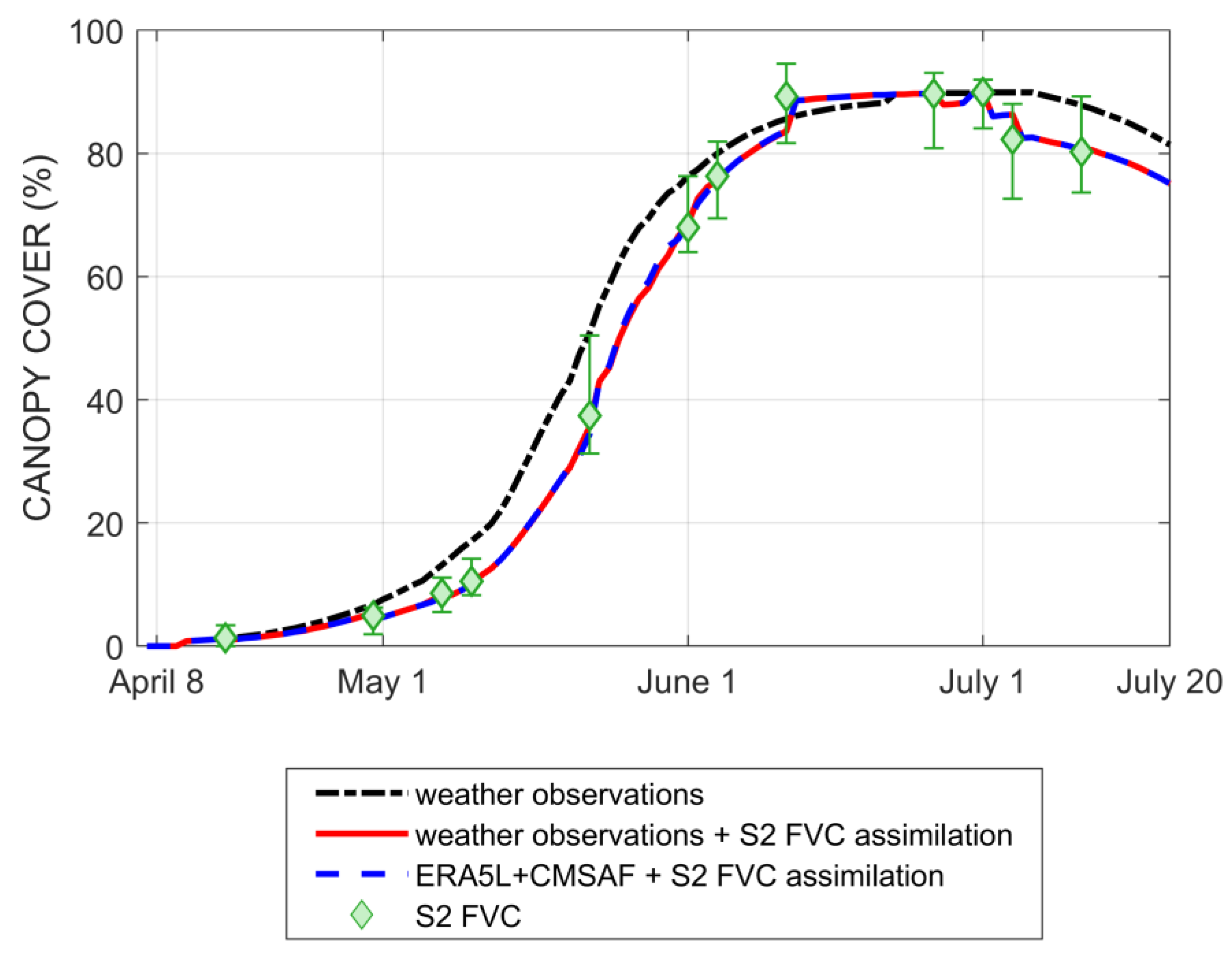
The following figures show two of the main variables of the AquaCrop model, i.e., canopy cover (
Figure 7) and crop evapotranspiration (
Figure 8) evolution during the crop growing cycle, for three input scenarios, as described above.
The first scenario, related to the availability of only weather observations, represents the basic scenario that can be implemented when only a weather station is available at a site of interest; no additional information is used to assess the growing process of the crop. However, the availability of satellite images for estimating the crop parameters (i.e., S2 FCV) is of tremendous relevance to AquaCrop simulations. Indeed, the availability of observed crop states during the growing cycle may improve estimates by assimilating the actual conditions of the crops into the model predictions as soon as the information becomes available. In this study, we corrected the AquaCrop CC evolution by assimilating the S2 FCV data (green diamonds on
Figure 7) via direct insertion, which resulted in an updated CC evolution that deviated from the first scenario model evolution.
Other interesting results regard the use of the merged ERA5-Land and CM-SAF database instead of weather observations, combined with S2 FCV data. In the CC evolution, scenario (iii) provided the same results as those obtained using weather observations and S2 FCV (scenario (ii)), since the main impact on the CC evolution is related to the assimilation of S2. Slight deviations in temperature (
Table 6) between the two inputs are not enough to influence the CC evolution.
Figure 7 also shows the assimilated values of S2 FCV on the 12 dates (
Table 2) of acquisition, along with error bars (representing the minimum and maximum values within the study plots), which are related to the uncertainty of estimates based on a given pixel. The first scenario provided CC values within the uncertainty range of variability of the S2 FCV only after June 1 during the fruit formation phase, while in the early growth, vegetative, and flowering phases, the gaps between CGM predictions and S2 FCV were significant.
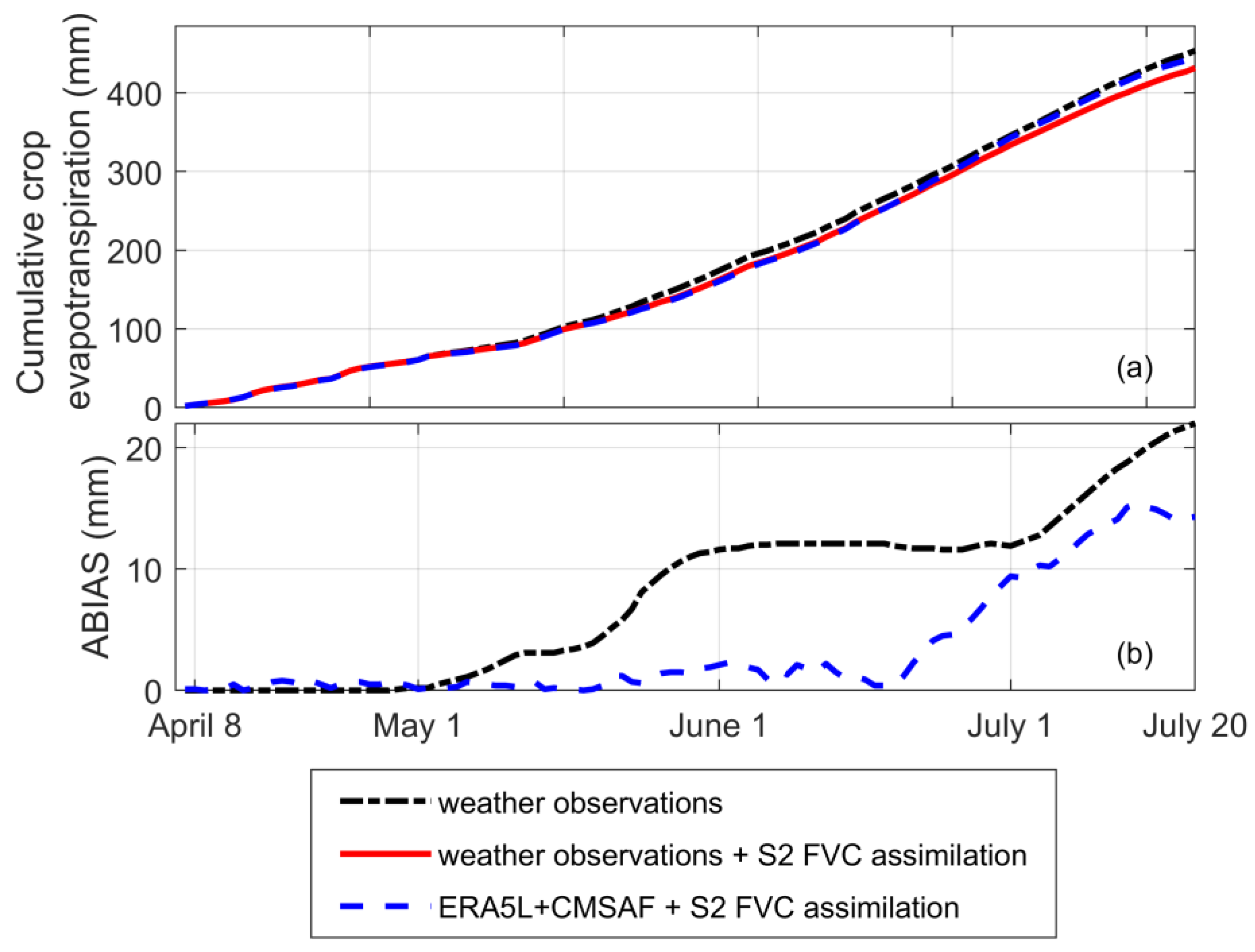
In
Figure 8, slight differences appear between the two scenarios that employed S2 FCV assimilation but different weather inputs, for the cumulative crop evapotranspiration evolution that depends on both CC and reference evapotranspiration. If we assume the second scenario to be a benchmark, the differences between the second and third scenarios are, on average, equal to 3.5%, and the cumulative ABIAS (
Figure 8b) is always below 15 mm (dashed blue line). The differences between the second and first scenarios is about 5%, while the cumulative ABIAS reaches 20 mm. No field data were available for a comparison of the crop evapotranspiration with the model results.
3.3. Crop Water Requirements and Yield
This section focuses on the main output of the model that was verified with field data (green color) for the three proposed scenarios.
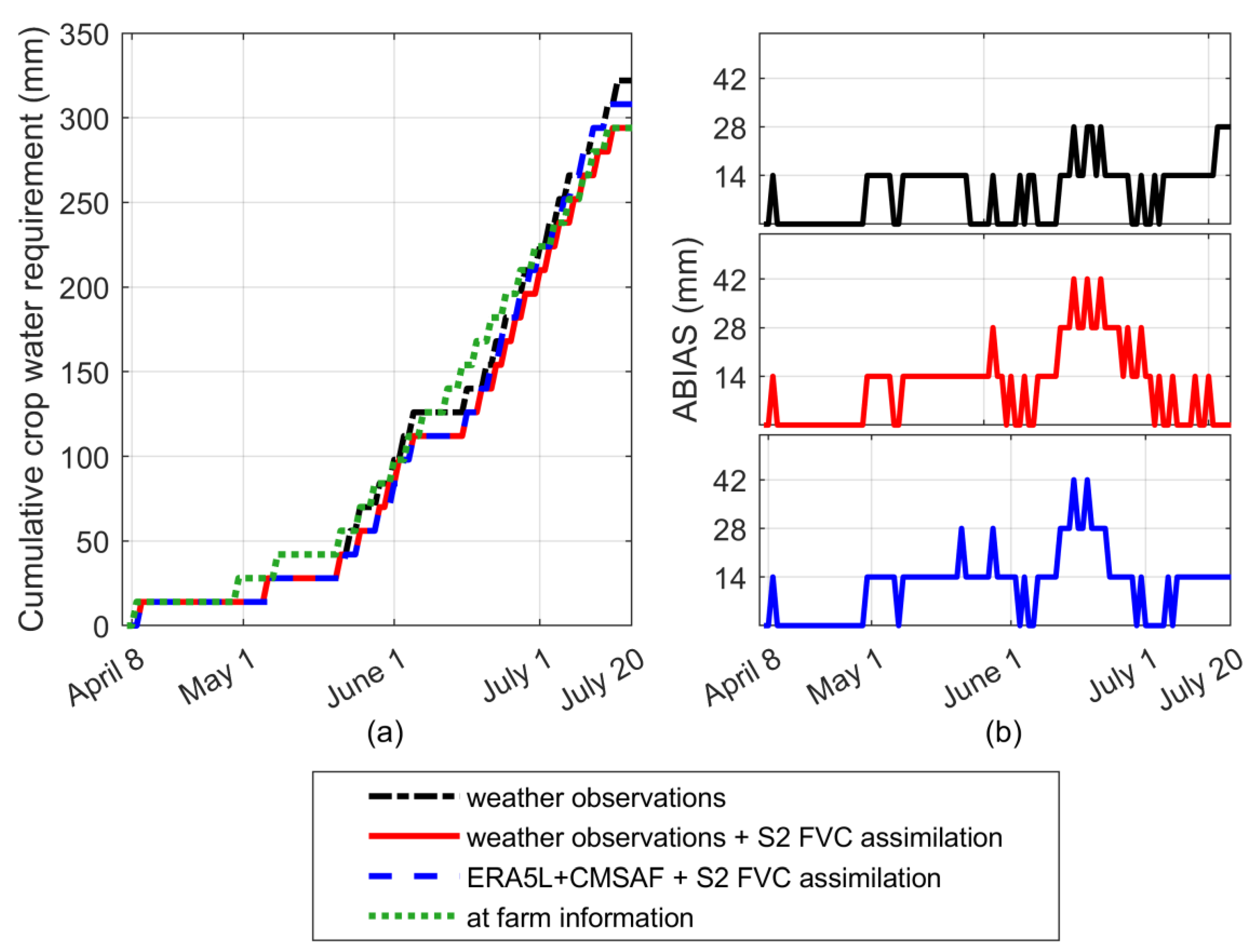
Figure 9a shows the cumulative irrigation depth, based on the optimal irrigation schedule generated with AquaCrop, compared with the actual irrigation schedule employed at the farm (green line). The cumulative crop water requirement can be conceptually assimilated with the irrigation volumes, in line with the hypotheses of this study.
Although the irrigation dates almost never coincide with the model proposal, the final irrigation volume is in perfect accordance with the model estimates for the scenario that uses ground weather observations and S2 FCV assimilation (i.e., scenario (ii)—red line). This outcome represents an important result if compared with the scenario that uses only weather observations (scenario (i)—black line), since it confirms that an important objective of the study was achieved, i.e., showing the importance of S2 FCV assimilation into the CGM simulations.
Moreover, the results are also encouraging for the third scenario (blue line), which achieved an ameliorated estimation of the final irrigation volume compared to the first scenario, confirming that the merged ERA5-Land and CM-SAF database represents a reliable and accurate remote proxy of ground weather observations if combined with S2 FCV assimilation. However, a slight overestimation of irrigation volumes was detected with respect to the first and third scenarios versus field data.
Figure 9b quantifies the cumulative ABIAS in irrigation depth estimates during the crop growing cycle for the three scenarios when compared to the field data. Although the final irrigation depth for the second scenario was the same as the field data, the misaligned irrigation dates determined an ABIAS of up to 42 mm (three irrigation events) during the growing cycle. Then, the ABIAS for the second scenario returned to zero. For the third scenario, the maximum ABIAS was equal to 42 mm, toward a final value of 14 mm, while for the first scenario, the maximum ABIAS was 28 mm, with the same final value. The best estimate was obtained in the second scenario, that improved the estimates of the first scenario thanks to the assimilation of S2 FCV, while the high level of accuracy of the estimates in the third scenario confirmed the positive effect of the merged ERA5-Land and CM-SAF database as a proxy of weather ground observations.
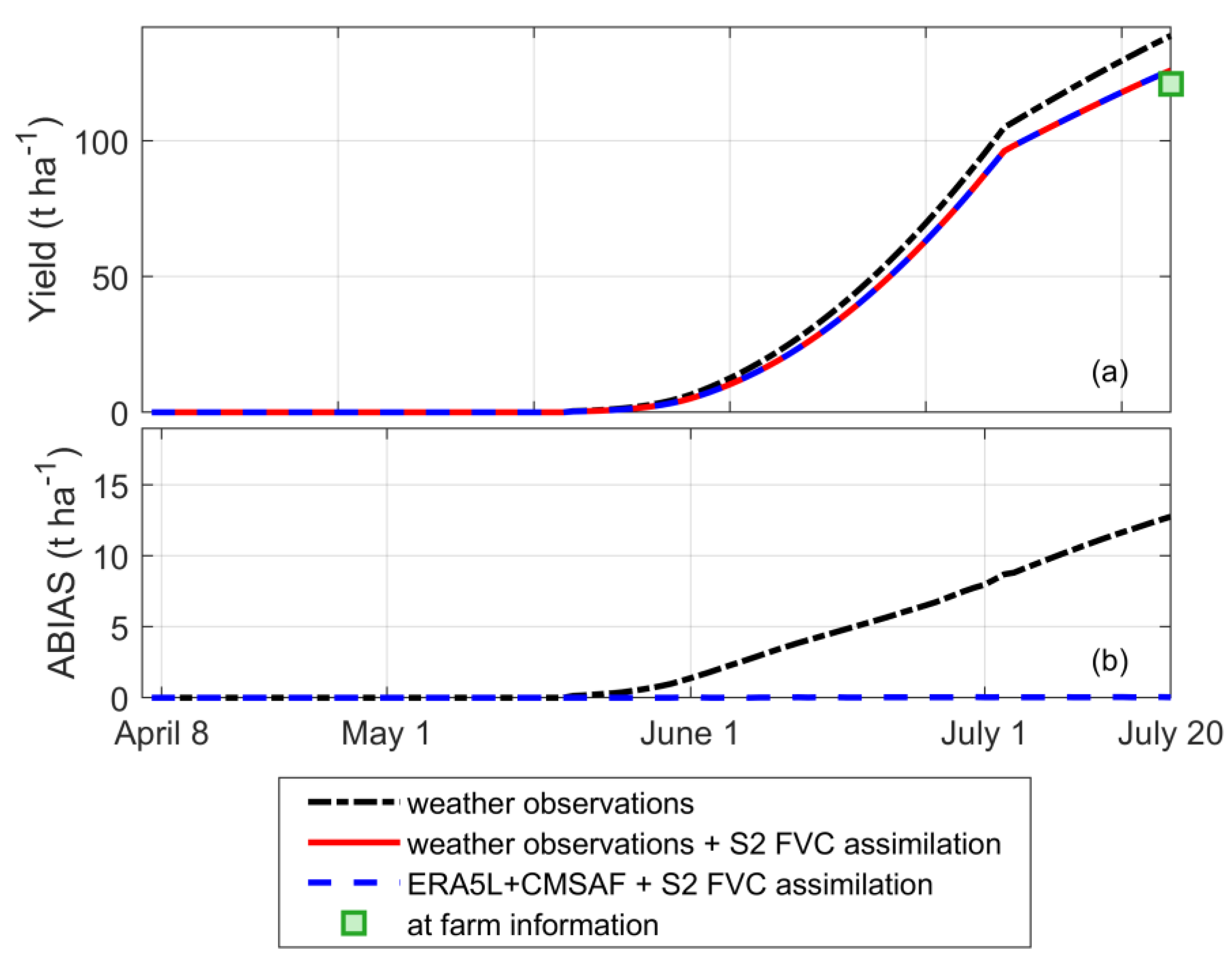
Figure 10 shows the AquaCrop outputs in terms of yield for the three scenarios (
Figure 10a).
Figure 10b displays the cumulative ABIAS of the first and third scenarios in comparison to the second. The second and third scenarios were basically equivalent in terms of yield estimates. The yield evolution differed between the first scenario and the other two in the final stage of the plant evolution (after 1 July, during the mature fruiting phase), while, in accordance with
Figure 7, the assimilation of S2 FCV brought about a major variation in the CC evolution, that would have been overestimated by the AquaCrop model itself (first scenario).
The benchmark for the validation was the final yield harvested at the end of the season (green circle on
Figure 10). As summarized in
Table 7, the first scenario overestimated the yield by about 14%, while the second and third scenarios overestimated by only 4%, showing a perfect accordance that further confirmed that the merged ERA5-Land and CM-SAF database represents a reliable and accurate remote proxy of ground weather observations if combined with S2 FCV assimilation.
4. Discussion and Conclusions
Knowledge of crop water requirements and yield under standard conditions, i.e., crops grown in large fields under excellent agronomic and soil water conditions [
5], is a fundamental requisite for addressing many water resource management issues, especially in areas such as Mediterranean regions, which are characterized by significant freshwater abstractions for crop irrigation during the dry seasons [
4].
Assessments of crop water requirements and yield necessitate multiple forms of input information, such as weather data and crop biophysical parameters, to implement crop–water balance models [
5]. The widespread development of EO systems [
13] and advances in numerical atmospheric modeling [
44] have opened to the opportunity of using new data sources, whose integration with models may significantly improve estimates. In this study, we investigated the ability of different input data from remote sensing and numerical sources to improve crop water requirement and yield estimates.
We gathered Sentinel-2 imagery to assess canopy cover during the growth cycle of processing tomato. Field measurements in the irrigation season of 2021 validated the satellite-based estimation with a RMSE equal to 11% and a coefficient of determination, R
2, equal to 0.987 (
Figure 6). Few studies have focused on this crop; however, similar results were found by [
30], who applied Sentinel-2 imagery to compute canopy cover for tomato in the same field in the irrigation seasons of 2018 and 2019. Another study with the same target crop used Sentinel-2 imagery to estimate the leaf area index and showed that the satellite estimations and the ground observations were significantly correlated, with R
2 = 0.689 and RMSE of 0.56 m
2/m
2 (25% of the mean value), confirming the high potential and quality of Sentinel-2 data for the retrieval of crop parameters [
55].
Many other studies that have used Sentinel-2 imagery for LAI and CC estimations may be found in literature for other types of crops; among these, it is worth mentioning the work by [
17] that assessed both LAI and CC for wheat in China. The authors found a better correlation and a smaller RMSE between satellite-based and ground observations for CC than for LAI estimates, due to the stronger influence of the presence of clouds and haze on LAI estimations. The RMSE related to the satellite-based estimates of CC for wheat was found to be 7.2%, in accordance with the results of the present study.
Regarding weather data, this study proposed a novel approach, i.e., the use of a merged ERA5-Land and CM-SAF database as a proxy of ground weather observations for the assessment of crop water requirements and yield. This merged database was previously tested in a recent study on the determination of reference values for evapotranspiration [
24]. The results showed that weather reanalysis, in particular ERA5-Land, provided a robust source for weather data; specifically, for solar radiation, weather estimates might be improved by replacing numerical reanalysis outputs with satellite-based estimates, e.g., CM-SAF, obtained by remote observations using the instruments onboard ESA Meteosat satellites, operated by EU-METSAT.
Sentinel-2 estimates of canopy cover and the weather database obtained by merging ERA5-Land reanalysis and CM-SAF were integrated with AquaCrop for the assessment of crop water requirements and yield. The AquaCrop model is a widely used agrohydrological model [
17]. Although it requires less input information than other types of models available in literature, such as CropSyst, WOFOST or EPIC model, it provides reliable predictions of optimal irrigation volumes and yield at harvesting [
10].
The results showed that Sentinel-2 estimates of crop parameters achieved enhanced accuracy. This study implemented an assimilation technique based on direct insertion; this technique does not consider the uncertainties of observations and crop model parameters. Further studies may be oriented toward the implementation of Bayesian data assimilation techniques producing the posterior probability distribution of the model predictions conditioned to the observations, as well to the structure of the errors in model parameters and observations [
18]. Moreover, the use of CGMs that can exploit LAI retrieved from Sentinel-2 as additional input crop parameters [
17] may represent an interesting future development that would be able to fully take advantage of the potential of satellite imagery for predicting crop development.
Complementary results showed that the merged ERA5-Land and CM-SAF weather database represents a reliable proxy of ground weather observations when combined with Sentinel-2 data. This finding is highly significant, since it gives rise to the possibility of using alternative weather gridded data in cases where ground weather data are not available. As shown in [
4], the spatial distribution of ground-based weather stations is generally too coarse and irregular for assessments of the spatial variability of the weather variables that are key inputs for CGM modeling. This consideration is even more valid for variables like solar radiation, whose spatial variability is commonly not captured by coarse networks of ground radiometers. Reanalysis databases and satellite-derived products, such as CM-SAF, represent alternative sources of weather data. Despite the spatial resolution of reanalysis data and satellite-derived products being relatively coarse (from 5 km to 10 km), recent studies have verified that the predictions produced with these data sources present performance similar to those that use interpolating ground-based weather observations in regions with relatively dense networks of weather stations [
4,
24].


