Article

Assessment of the Steering Precision of a UAV along the Flight Profiles Using a GNSS RTK Receiver

1
Department of Geodesy and Oceanography, Gdynia Maritime University, Morska 81-87, 81-225 Gdynia, Poland
2
Department of Transport and Logistics, Gdynia Maritime University, Morska 81-87, 81-225 Gdynia, Poland
*
Author to whom correspondence should be addressed.
Remote Sens. 2022, 14(23), 6127; https://doi.org/10.3390/rs14236127
Submission received: 9 November 2022 / Revised: 28 November 2022 / Accepted: 29 November 2022 / Published: 2 December 2022
(This article belongs to the Special Issue GNSS CORS Application)

Abstract

:
Photogrammetric surveys are increasingly being carried out using Unmanned Aerial Vehicles (UAV). Steering drones along the flight profiles is one of the main factors that determines the quality of the compiled photogrammetric products. The aim of this article is to present a methodology for performing and processing measurements, which are used in order to determine the accuracy of steering any drone along flight profiles. The study used a drone equipped with a Global Navigation Satellite System (GNSS) Real Time Kinematic (RTK) receiver. The measurements were performed on two routes which comprised parallel profiles distant from each other by 10 m and 20 m. The study was conducted under favourable meteorological conditions (windless and sunny weather) at three speeds (10 km/h, 20 km/h and 30 km/h). The cross track error (XTE), which is the distance between a UAV’s position and the flight profile, calculated transversely to the course, was adopted as the accuracy measure of steering a UAV along the flight profiles. Based on the results obtained, it must be concluded that the values of XTE measures for two representative routes are very similar and are not determined by the flight speed. The XTE68 measure (p = 0.68) ranged from 0.39 m to 1.00 m, while the XTE95 measure (p = 0.95) ranged from 0.60 m to 1.22 m. Moreover, analyses demonstrated that the statistical distribution of the XTE measure was most similar to the gamma and Weibull (3P) distributions.

1. Introduction

An Unmanned Aerial Vehicle (UAV) is an aircraft capable of performing a flight with no pilot on board. Therefore, the aircraft’s flight must be performed autonomously, in pre-programmed mode, or using remote control. Another commonly used term for a UAV is a drone [1].
Originally, UAVs were used for military applications such as land mapping, surveillance zone, performing reconnaissance and as long-range weapons. Nowadays, drones are used in many different areas, including civilian applications. Compared to classical solutions, i.e., manned aerial vehicles, UAVs are characterised by significantly lower operating costs. The fact that drones offer a cheaper alternative has helped UAVs revolutionise the aeronautics industry [1,2,3].
The most important factors that affect the development of drones are the continuous advances being made in the field of microelectronics, radio technology and miniaturisation. UAVs are characterised by their high manoeuvrability, small size and high availability, as well as they enable the performance of complex tasks. Due to the continued development of drones for civilian applications, the number of sectors using UAVs is increasing, which contributes to their universality and the continued expansion of their capabilities. The main areas of drone application include [3,4]: archaeology and architecture [5,6,7,8,9], agriculture [10,11,12,13,14], crisis management [15,16,17,18,19], environment [20,21,22,23,24,25], forestry [26,27,28,29,30], as well as traffic monitoring [31,32,33,34,35]. In order to use a UAV in the above-mentioned applications, it is necessary to know its accuracy of steering along the flight profiles. This parameter is very important from the point of view of ensuring navigational safety [36]. Presented below are the results of several research during which the accuracy of steering a drone was determined.
Bhattacherjee et al. [37] used Radio Frequency (RF) sensors to detect and locate UAVs through passive monitoring of signals emitted by drones. Moreover, the errors of steering a UAV along the flight profiles were filtered using the Extended Kalman Filter (EKF). The study used Keysight N6854A RF sensors and DJI Inspire 2 drone. The measurements were performed in an open area in Dorothea Dix Park (Raleigh, NC, USA). The study demonstrated that depending on the measurement section, the accuracy of steering a UAV along the flight profiles amounted to 4.76 m (standard deviation) when using the EKF filter and 6.6 m (standard deviation) when using RF sensors.
Brunet et al. [38] developed a method for detecting, tracking and controlling the UAV’s flight parameters based on a stereo image. The study used a multi-engine drone equipped with oCamS-1CGN-U stereo camera and RotorS simulator proposed by Furrer et al. [39], as well as Micro Aerial Vehicle (MAV) virtual environment. Simulation tests demonstrated that the accuracy of steering a UAV along a 3D spiral route amounted, in the best case, to 0.09 m (Root Mean Square (RMS)).
Connor et al. [40] used a UAV to compile 3D maps of radiation in the Fukushima region (Ōkuma, Japan). Their study used a lightweight (3 kg) quadrocopter equipped with Pixhawk autopilot and Go Pro Hero 5 Black camera. The experimental tests demonstrated that the accuracy of steering a UAV along the parallel flight profiles (distant from each other by 1.5 m) was, on average, 0.47–0.68 m, while the max deviation of the drone from the planned route ranged from 0.91 m to 1.02 m.
Goel et al. [41] developed a new cooperative location prototype which uses the exchange of information between a UAV and static anchor nodes in order to precise positioning of the drone. The study used an octocopter equipped with Pixhawk autopilot, GoPro camera, Raspberry Pi 3 computer, GPS u-blox receiver, UWB P410 radio and a modem for communication and data transmission. The experimental tests demonstrated that the designed system allows the UAV’s positioning accuracy to be obtained at a level of 2–4 m in the absence of a GNSS signal, provided that continuous communication is ensured in the cooperative network.
Nemra and Aouf [42] presented a new Global Positioning System (GPS)/Inertial Navigation System (INS) data fusion scheme based on the nonlinear State-Dependent Riccati Equation (SDRE) filter used to locate UAVs. The simulation tests demonstrated that the SDRE algorithm enables more accurate steering of a drone along the planned route as compared to the Kalman Filter (KF), EKF and Unscented Kalman Filter (UKF) algorithms. The accuracy of steering a UAV along the flight profiles amounted to: 4.05 m (RMSx), 1.26 m (RMSy) and 3.07 m (RMSz) for the SDRE algorithm.
Paraforos et al. [43] presented a methodology for determining the positioning accuracy of images taken by a UAV. For this purpose, the authors used a prismatic mirror installed on the drone, tracked by a total station. The study used DJI Matrice 100 drone, Parrot Sequoia + multi-spectral camera, Trimble 360 Prism prismatic mirror, GNSS receiver receiving corrections from EGNOS system and Trimble SPS930 total station. The measurements were conducted at University of Hohenheim (Hohenheim, Germany). Experimental studies demonstrated that the accuracy of steering a UAV along the flight profiles (cross track error (XTE)) in the 2D plane amounted to 0.65 m (standard deviation) and 2.33 m (p = 0.95).
Shah et al. [44] presented a sliding mode based lateral (cross-track) control scheme along straight and circular sections for UAVs. The system is designed to minimise the XTE error, i.e., the distance between a UAV’s position and the planned route. Simulation tests demonstrated that the XTE error of a UAV on 400-metre straight sections did not exceed 5 m, while on curved sections, it was approx. 2 m.
Vílez et al. [45] developed an algorithm for trajectory generation and flight tracking using the Robot Operating System (ROS) for AR.Drone 2.0 quadrocopter. To design the flight route, Bézier curves and third-degree polynomials were used. The study performed 40 simulations using the Gazebo simulator and 46 real measurements for different flight trajectories. The tests demonstrated that the greatest mean error of steering a UAV along the flight profiles with a length of 40 m was 2.8 m (simulation) and 5.06 m (real measurements) if the Bézier curves were used for flight trajectory modelling. However, the greatest mean error of steering a UAV along the flight profiles with a length of 60 m was 3.73 m (simulation) and 5.13 m (real measurements) if third degree polynomials were used for flight trajectory modelling.
Yang et al. [46] used UAVs for the inspection of transmission lines. The authors noted wind gusts which have an adverse effect on the steering of a drone along the planned route. The article proposed a sliding mode robust adaptive control algorithm for an aerial vehicle to solve this problem. Simulation tests used a UAV equipped with PX4 autopilot and GPS u-blox NEO-M8N receiver. Tests demonstrated that the accuracy of steering a UAV along the flight profiles was: 0.16–0.21 m (for the northing), 0.31–0.58 m (for the easting) and 0.63–1.21 m (for the height).
Yang et al. [47] proposed a nonlinear double model for multisensor-integrated navigation using the Federated Double-Model EKF (FDMEKF) for small UAVs. The proposed algorithm was compared to other existing filters (Multi-Sensor Complementary Filtering (MSCF) and Multi-Sensor EKF (MSEKF)) using the data derived from different instruments. Experimental tests demonstrated that in terms of the accuracy of steering a UAV along the planned route, the proposed filtering method (FDMEKF) was more accurate than the MSCF and MSEKF filters. The accuracy of steering a UAV along the flight profiles amounted to: 0.658 m (standard deviation) and 0.223 m (RMS) (for the northing), 0.503 m (standard deviation) and 0.523 m (RMS) (for the easting), as well as 0.691 m (standard deviation) and 0.512 m (RMS) (for the height) for the FDMEKF algorithm.
Based on the review of the literature, it should be stated that the accuracy of steering a UAV depends on many factors, such as the type of drone, positioning system, weather conditions, etc. Therefore, the aim of this article is to present a methodology for performing and processing measurements, which are used to calculate the accuracy of steering any UAV along flight profiles. It was also decided to determine the impact of the speed and shape of the route on the accuracy of steering a drone supported by the GNSS RTK receiver.
This article is structured as follows: Section 2 describes the measurement equipment (UAV and GNSS RTK receiver) used when performing the photogrammetric surveys. Moreover, this section presents the photogrammetric survey planning and performance, as well as specifies how the data recorded during the measurements were compiled. Section 3 calculates the accuracy measures of steering a UAV along the flight profiles (XTE68 and XTE95) and determines the statistical distributions that are best fitted to the XTE distributions. The paper concludes with final (general and detailed) conclusions that summarise its content.

2. Materials and Methods

2.1. Measurement Equipment

DJI Phantom 4 RTK is a quadrocopter from a popular Phantom series and its first representative from the DJI Enterprise segment. This is all thanks to the RTK module, which is directly integrated with a drone and provides real-time positioning data with one-centimetre accuracy to improve the accuracy of image metadata. Omnidirectional obstacle detection was achieved thanks to intelligent obstacle detection sensors during both outdoor and indoor flights. The UAV has a 24 mm wide-angle lens (35 mm equivalent focal length). Photos and films are recorded on a 1” Complementary Metal-Oxide-Semiconductor (CMOS) sensor with a resolution of 20 Mpx. The camera has a mechanical shutter, which allows a series of images to be taken efficiently without the risk of blurring. The technical data of DJI Phantom 4 RTK drone, along with DJI camera pre-installed on it, are presented in Table 1 and Table 2.
As regards the GNSS RTK receiver, DJI company provided no detailed information on the device model. The manufacturer’s website only mentions that the receiver has the ability to track signals transmitted by satellites of the following systems: GPS (L1/L2), GLObal Navigation Satellite System (GLONASS) (L1/L2), BeiDou Navigation Satellite System (BDS) (B1/B2) and Galileo (E1/E5a). However, the positioning accuracy is 1 cm + 1 ppm (RMS) in the horizontal plane and 1.5 cm + 1 ppm (RMS) in the vertical plane.

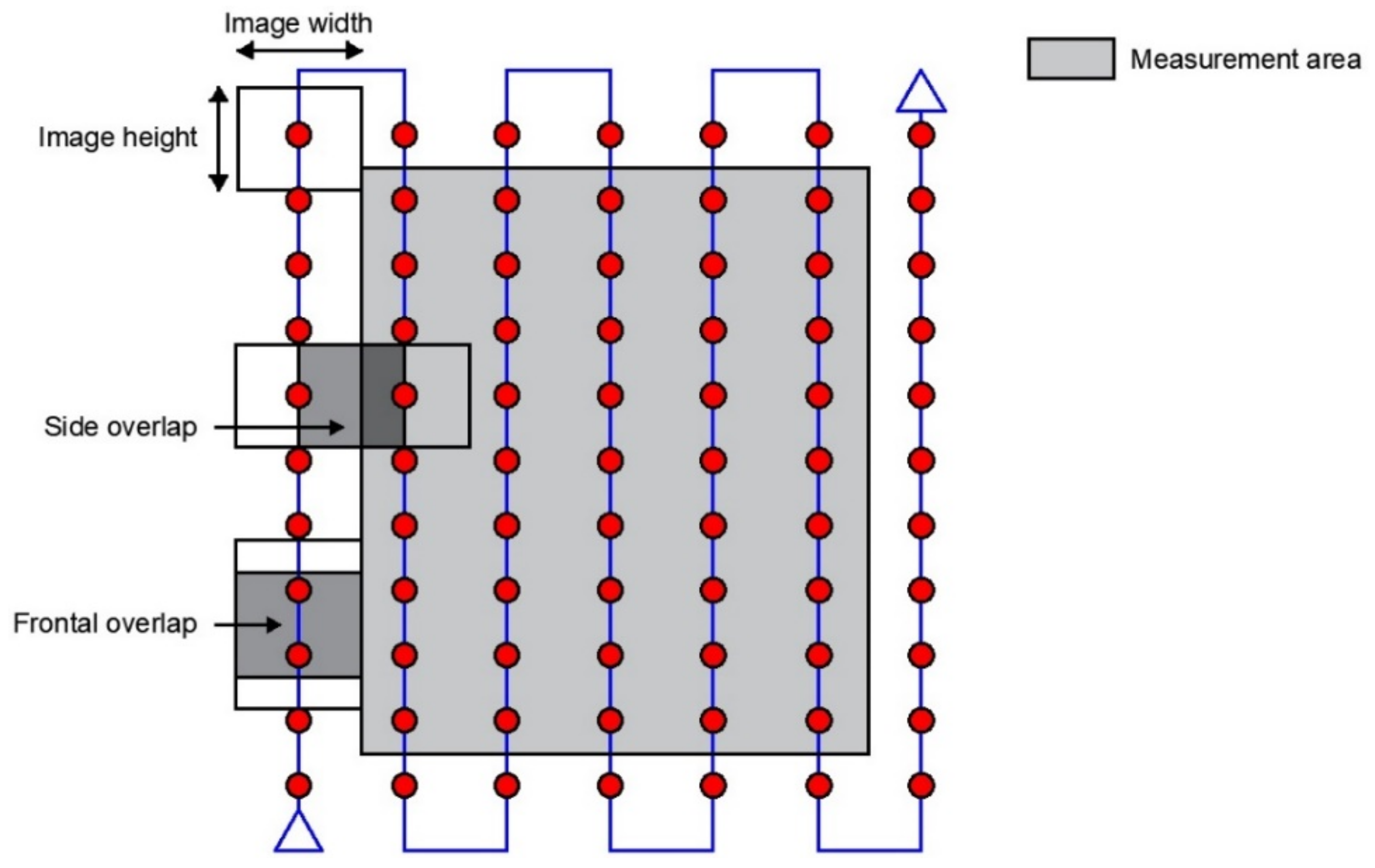
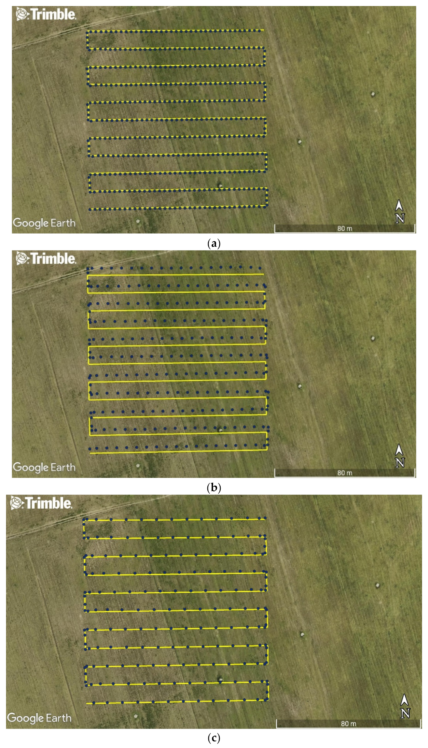
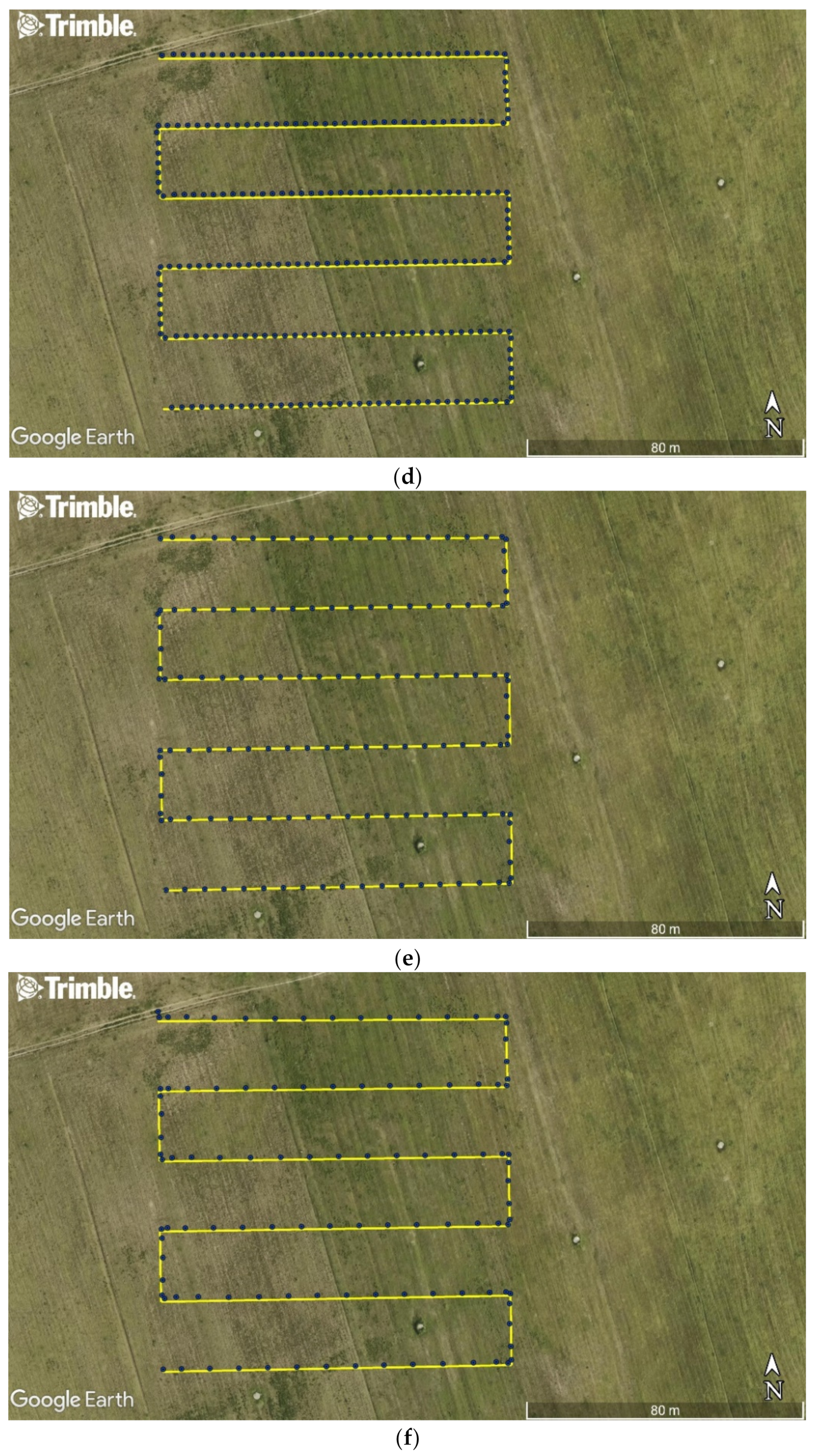
2.2. Photogrammetric Survey Planning and Performance

Before starting the study, it was necessary to specify the longitudinal (oforward) and transverse (oside) coverage of images, distance between flight profiles (dside), camera height above the ground surface (H), flight speed (V) and Ground Sample Distance (GSD). As a first step, it was decided to determine the longitudinal and transverse coverage of images (Figure 1), which can be calculated using the following formulas [48,49]:
o f o r w a r d = 1 d f o r w a r d f H w 100 %
o s i d e = 1 d s i d e f H w 100 %
where:
  • oforward—longitudinal coverage of images (%),
  • oside—transverse coverage of images (%),
  • dforward—distance between successive images (m),
  • dside—distance between flight profiles (m),
  • f—camera focal length (mm),
  • H—camera height above the ground surface (m),
  • w—camera sensor width (mm) [50].
Figure 1. The graphic interpretation of the longitudinal and transverse coverage of images.
Remotesensing 14 06127 g001
The longitudinal coverage of images should be at least 70–90%, while the transverse coverage of images must not be less than 60–80% [51,52]. For the purposes of the photogrammetric surveys, both the longitudinal and transverse coverage of images was assumed to be 70%.
Another parameter to be set was the flight speed. It follows from the literature review [53,54,55,56] that the UAV’s photogrammetric flights can be performed at speeds as high as 50–70 km/h. Since the operational speed of DJI Phantom 4 RTK drone is approx. 25 km/h, it was decided to carry out the study at three speeds of: 10 km/h (2.8 m/s), 20 km/h (5.6 m/s) and 30 km/h (8.3 m/s).
The camera height above the ground surface (H) could then be determined. In order to perform the flight along the planned routes at three speeds: 10 km/h, 20 km/h and 30 km/h, it was necessary to set the height H at 105 m. UAV photogrammetric flights are commonly performed at heights of approx. 100 m, as they allow the GSD at a level of 2–3 cm to be obtained [57,58]. The ground sample distance can be calculated using the following formula:
G S D = H w f i w
where:
  • GSD—field pixel size (cm/px),
  • iW—image width (px).
When the longitudinal coverage of images (oforward), camera height above the ground surface (H) and selected technical parameters of the camera used (w = 25.4 mm and f = 24 mm) were known, the min. distance between the flight profiles (dforward) could be calculated using the following relationship:
d f o r w a r d = 100 % o f o r w a r d H w f
The routes were designed in such a manner that the flight profiles were parallel to each other. Based on the relationship (4), it was assumed that the mutual distance between the flight profiles would be 10 m (Figure 2a–c) and 20 m (Figure 2d–f).
The routes were designed using the Trimble Business Center (TBC) software. The coordinates of the route turning points were then exported to files with the extension *.kml. These points were recorded as geodetic coordinates referenced to the World Geodetic System 1984 (WGS-84) ellipsoid with an accuracy of eight decimal places. The planned UAV routes set in this manner was uploaded to the dedicated DJI Go software. The program is used for planning routes on which UAVs can move in automatic/autonomous mode. In this way, the prepared data are sent via Wi-Fi and Bluetooth modules from the drone’s control unit, on which the DJI Go software is installed, to the unmanned aerial vehicle. After setting all the necessary default parameters, the flight along the set points in automatic mode could be started.
On 9 August 2022, the photogrammetric surveys were performed to assess the accuracy of steering a UAV along the flight profiles. Moreover, an attempt was made to determine the optimal trajectory of the drone’s movement, with the parallel profile method subjected to verification. It was decided to carry out the study at an airport dedicated to unmanned aircraft in Gdynia (Poland). Since the meteorological conditions can significantly affect the obtained results, the measurements were performed under suitable weather conditions, i.e., no precipitation, windless weather (wind speed not exceeding 6–7 m/s) and sunny day. Such conditions allowed clear, evenly lit images to be taken. In addition, the receiver used the nearest reference station (located in Gdańsk) of the VRSNet.pl GNSS geodetic network to generate RTK corrections. Thanks to them, it is possible to determine position coordinates of a UAV with an accuracy of 1–1.5 cm (RMS) in the horizontal and vertical planes. Moreover, in order to assess the accuracy of steering a UAV along the flight profiles, it is necessary to determine the position data sampling frequency [59]. The value of this parameter is dependent on the GNSS receiver that is installed on the drone. Similar to other studies conducted by other authors [60,61], it was decided to record position data at a frequency of 1 Hz.

2.3. Data Processing

During the photogrammetric surveys, the GNSS RTK receiver recorded its position coordinates in relation to the WGS-84 ellipsoid. In order to calculate the distances between the designed routes and the routes covered by the UAV, it was decided to convert the measured coordinates into a uniform reference system to enable the determination of the XTE value in metres. Therefore, it was decided to transform coordinates to the PL-2000 system, which, in accordance with the ordinance of the Council of Ministers on the national spatial reference system, has been the basic geodetic coordinate system in force in Poland since 2012 [62]. The angular coordinates were converted into Cartesian coordinates in the PL-2000 system based on the following mathematical relationships [61,63]:
x = m 0 N S ( B ) N + ( Δ L ) 2 2 sin ( B ) cos ( B ) + ( Δ L ) 4 24 sin ( B ) cos 3 ( B ) ( 5 t 2 + 9 η 2 + 4 η 4 ) + + ( Δ L ) 6 720 sin ( B ) cos 5 ( B ) ( 61 58 t 2 + t 4 + 270 η 2 330 η 2 t 2 + 445 η 4
y = m 0 N Δ L cos ( B ) + ( Δ L ) 3 6 cos 3 ( B ) ( 1 t 2 + η 2 ) + + ( Δ L ) 5 120 cos 5 ( B ) ( 5 18 t 2 + t 4 + 14 η 2 58 η 2 t 2 + 13 η ) + 500,000 + L 0 3 1,000,000
where:
  • m0—scale factor (–),
  • N—ellipsoid normal (radius of curvature perpendicular to the meridian) (m),
  • S(B)—meridian arc length from the equator to the arbitrary latitude (B) (m),
  • ΔL—distance between the point and the central meridian (rad),
  • B,L—ellipsoidal coordinates of the point (°),
  • L0—longitude of the central meridian (°),
The other parameters of projection to the two-dimensional (2D) Cartesian coordinates in the PL-2000 system include:
t = tan B
η = e 2 cos 2 ( B ) 1 e 2
where:
  • η—ellipse distortion orientation angle (−),
  • e—first eccentricity (−).
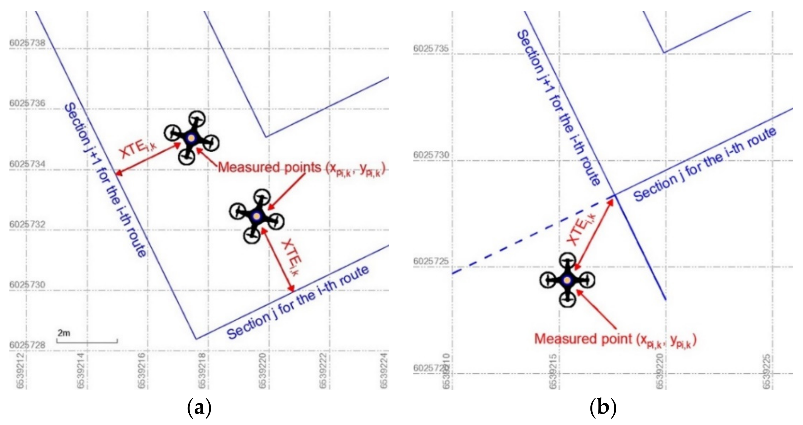
The distance between the designed routes and the routes covered by the UAV then had to be calculated. The article defined it using the XTE measure, i.e., the distance that is determined between a UAV’s position and the flight profile, which is measured transversely to the course. The concept of the XTE measure can be found in [61,64]. In order to determine this variable, it was necessary to describe each route mathematically. As they only comprised straight sections, each segment of the route could be represented using the linear function expressed with the following formula:
x i , j = a i , j y i , j + b i , j
where:
  • i—route number (−),
  • j—section number of the i-th route (−),
  • xi,j, yi,j—flat coordinates of the point j recorded by a GNSS RTK receiver on the i-th route in the PL-2000 system (m),
  • ai,j—slope of the straight line j for the i-th route, defined as follows (−):
a i , j = x i , j + 1 x i , j y i , j + 1 y i , j
  • bi,j—y-intercept of the straight line j for the i-th route, defined as follows (m):
b i , j = x i , j a i , j y i , j
Once the course of each segment of the designed route had been mathematically determined, it was possible to calculate the distances between the designed routes and the routes covered by the UAV. However, two variants had to be considered when performing the calculations. In the first of them, a straight line perpendicular to the designed route segment could be drawn through the measurement point (Figure 3a), which was not possible in the second variant (Figure 3b). Variant I determines the distance between a measurement point and the designed route segment using the following formula:
X T E i , k = a i , j y p i , k + x p i , k b i , j a i , j 2 + 1
where:
  • k—point number recorded by a GNSS RTK receiver (−),
  • x p i , k , y p i , k —flat coordinates of the point k recorded by a GNSS RTK receiver on the i-th route in the PL-2000 system (m).
However, variant II calculates the distance to the nearest turning point using the following formula:
X T E i , k = x p i , k x i , j 2 + y p i , k y i , j 2
Figure 3. The graphical method for determining the distance between the measurement point and the designed route for variants I (a) and II (b).
Remotesensing 14 06127 g003

3. Results

After calculating the distances between the designed routes and the routes covered by the UAV, a statistical analysis of this variable was conducted. To this end, two accuracy measures were determined: XTE68 and XTE95. They describe which value is not exceeded by 68% (XTE68) and 95% (XTE95) of the distances between the designed routes and the routes covered by a UAV [61]. The values of the XTE68 and XTE95 measures for the routes comprising parallel profiles distant from each other by 10 m (Table 3) and 20 m (Table 4) are presented below.
The study also analysed the distribution of a random variable, i.e., the distance between the designed route and the route recorded by a GNSS RTK receiver. To this end, the free software Easy Fit was used, which checks, by means of statistical tests such as the Anderson-Darling test, chi-square test and Kolmogorov-Smirnov test [65,66,67,68], whether the distribution of a random variable in the population differs from the assumed theoretical distribution. The program then classifies the probability distributions according to the obtained statistics for the particular statistical tests [61]. For the purposes of the study, the most commonly used theoretical distributions in navigation were used: Beta, Cauchy, chi-square, exponential, gamma, Laplace, logistic, lognormal, normal, Pareto, Rayleigh, Student’s and Weibull [69,70,71,72]. Moreover, the statistical analyses ignored the results obtained on the route comprising parallel profiles distant from each other by 10 m at a speed of 20 km/h (Figure 2b) due to the lack of sample representativeness. It follows from the conducted analyses that the empirical distribution of the distances between the designed routes and the routes covered by the UAV is the most similar to the gamma distribution (Kolmogorov-Smirnov test) and Weibull (3P) distribution (Anderson-Darling and chi-square tests). Similar results of the studies into the empirical distributions of navigation positioning system errors were obtained in [69,70,71,72].
The Cumulative Distribution Function (CDF) of the two-parameter gamma distribution of the XTE variable is expressed by the following formula [73,74]:
F XTE = Γ XTE α g Γ α g
where:
  • αg—gamma shape parameter (αg > 0) (−),
  • βg—gamma scale parameter (βg > 0) (−),
  • Γg)—gamma function defined as follows (−):
Γ α g = 0 t α g 1 e t d t
  • ΓXTE(αg)—incomplete gamma function defined as follows (−):
Γ XTE α g = 0 XTE t α g 1 e t d t
The CDF of the three-parameter Weibull distribution of the XTE variable is expressed by the following formula [75,76]:
G XTE = 1 e XTE γ β w α w
where:
  • αw—Weibull shape parameter (αw > 0) (−),
  • βw—Weibull scale parameter (βw > 0) (−),
  • γ—location parameter (XTE ≥ γ) (−).
CDFs of the gamma and Weibull (3P) distributions of the XTE variable are presented on the graphs generated by the Easy Fit software (Figure 4).
In statistics and probability calculus, the value of the XTEp is referred to as the quantile of the order p, where 0 ≤ p ≤ 1, in the empirical distribution PXTE of the XTE variable, for which the following inequalities are met:
P XTE , XTE p p
P XTE XTE p , + 1 p
where:
  • p—probability of the XTE variable occurring in the population under study (−).
In the next stage of the work, it was decided to determine how much the empirical CDF differs from the theoretical one for the particular distributions. To this end, the differences between the probabilities of the XTE variable occurrence for the empirical and theoretical gamma (Δpg(XTE)) and Weibull (3P) (Δpw(XTE)) distributions were calculated using the following formulas:
Δ p g XTE = F n XTE F XTE
Δ p w XTE = G n XTE G XTE
where:
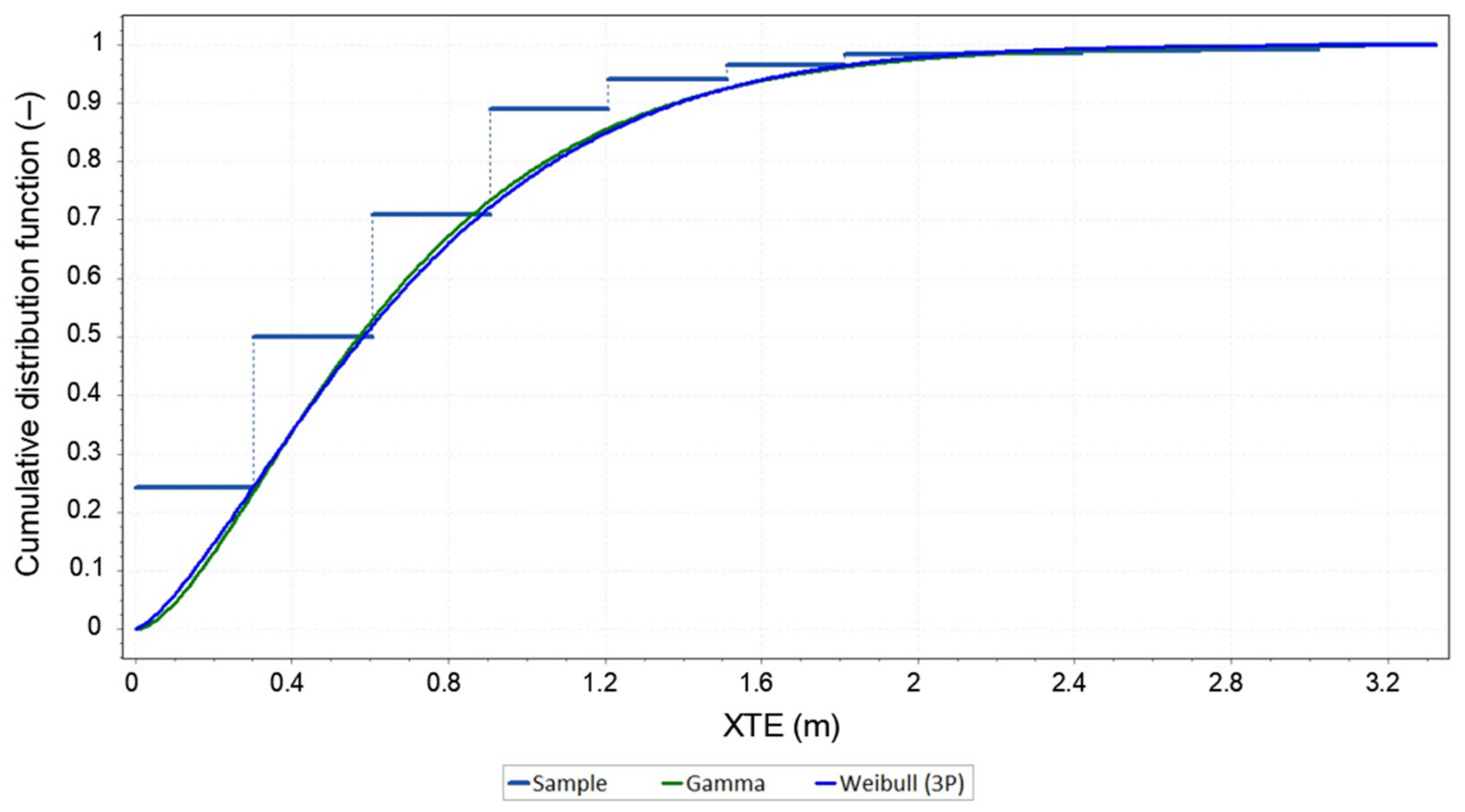
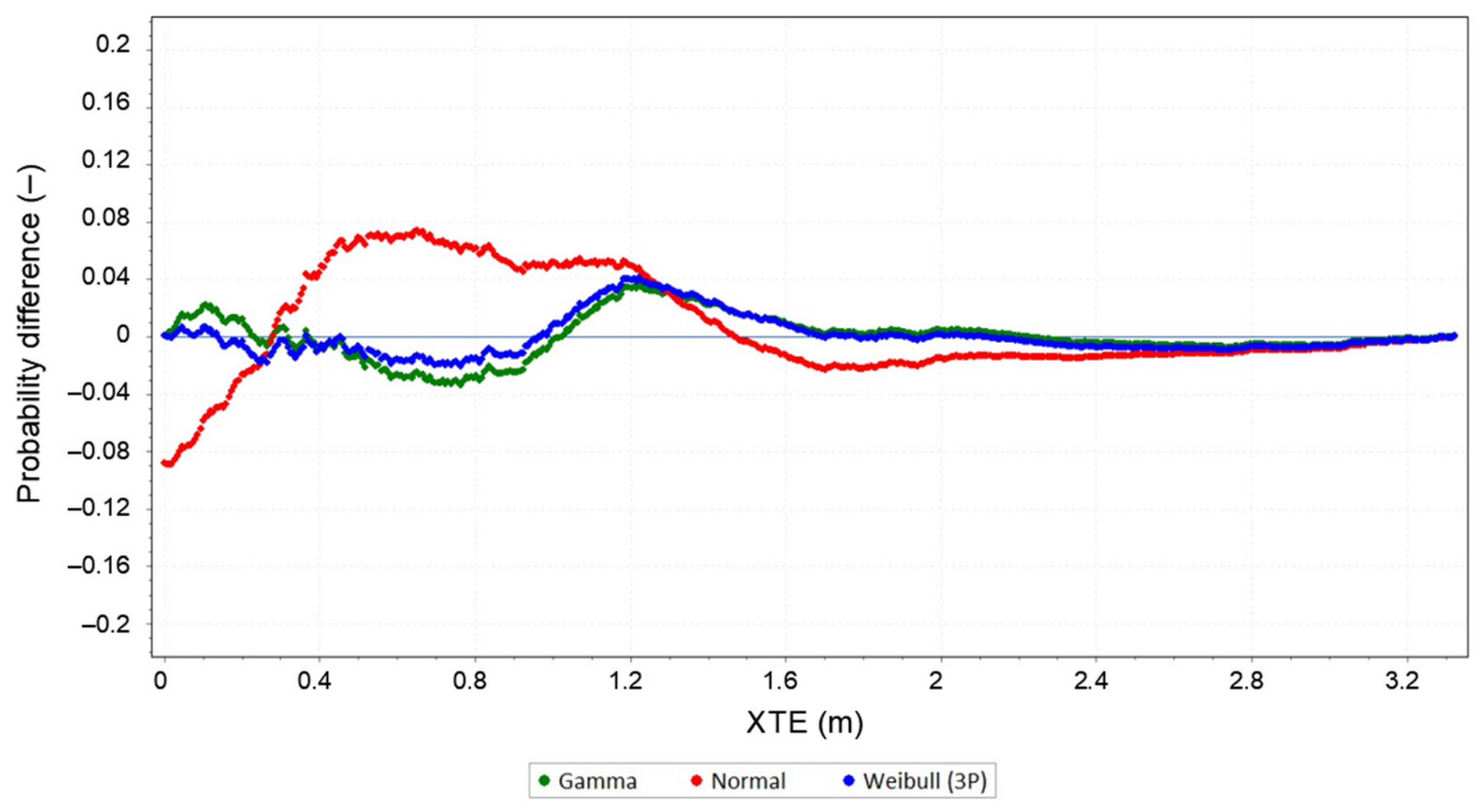
  • Fn(XTE)—empirical CDF of the gamma distribution of the XTE variable (−),
  • F(XTE)—theoretical CDF of the gamma distribution of the XTE variable (−),
  • Gn(XTE)—empirical CDF of the Weibull (3P) distribution of the XTE variable (−),
  • G(XTE)—theoretical CDF of the Weibull (3P) distribution of the XTE variable (−).
The graph of the differences between the probabilities of the XTE variable occurrence for the empirical and theoretical gamma, Weibull (3P) and normal distributions is provided in Figure 5.

4. Discussion

Based on the results presented in Table 3 and Table 4, it must be concluded that the values of accuracy measures of steering a UAV for two representative routes are very similar to each other and are not determined by the flight speed. The differences between the particular XTE68 (0.39–1.00 m) and XTE95 (0.60–1.22 m) errors were approx. 60 cm for a GNSS RTK receiver. Moreover, the statistical analyses ignored the results obtained on the route comprising parallel profiles distant from each other by 10 m at a speed of 20 km/h (Figure 2b) due to the lack of sample representativeness. This resulted from the fact that the photogrammetric flight was performed 3 or 4 h later than the other flights due to the discharge of all available batteries powering the drone. Despite the almost identical measurement conditions (the only difference was the wind direction and force), the values of accuracy measures XTE68 (3.94 m) and XTE95 (4.17 m) were four times greater than the metrics obtained on the other routes.
On the basis of Figure 4, it can be concluded that the quantiles of the order of 0.68 and 0.95 (percentiles) of the XTE variable for the gamma distribution amount to 0.81 m and 1.70 m, respectively. Moreover, the quantiles of the order of 0.68 and 0.95 of the XTE variable for the Weibull (3P) distribution amount to 0.83 m and 1.68 m, respectively. This should be interpreted to mean that 68% of the distances between the designed routes and the routes covered by the UAV is not greater than 0.81 m or 0.83 m and, similarly, 95% of the elements of this population do not exceed the value of 1.68 m or 1.70 m.
Based on Figure 5, it can be observed that the empirical and theoretical distributions for the gamma and Weibull (3P) distributions are characterised by a high degree of fit. The max difference between the probabilities of the XTE variable occurrence for the empirical and theoretical gamma and Weibull (3P) distributions ranges from −0.02 to 0.04. However, for normal (Gaussian) distribution, which is the most important theoretical probability distribution used in statistics, the analysed measure is several times larger and amounts to approx. ±0.08.

5. Conclusions

The accuracy of steering a UAV along the flight profiles is very important from the point of view of ensuring navigational safety [36]. Due to the low accuracy of steering a UAV (keeping it on the profile), dangerous situations may occur, such as collision with people, resulting in severe damages and/or injuries [77,78,79], collision with static and other flying objects, e.g., buildings and powerlines, other UAVs, as well as manned aircraft [77,78], or flights in restricted zones [80].
Research results have shown that GNSS RTK receivers can be successfully used in UAVs for applications related to, among others, archaeology and architecture, crisis management, forestry, photogrammetric surveys, precision agriculture, or in traffic monitoring [80,81].
The study proved that the use of a GNSS RTK receiver would allow high accuracy of steering a UAV along the flight profiles to be achieved despite many factors that affect it. These include, e.g., initial state errors, intent update errors, dynamic intent updates, vehicle performance errors, weather forecast or trajectory modelling errors [59,81,82,83]. As part of future research, it is planned to determine the effect of the above-mentioned factors on the accuracy of steering a UAV along the flight profiles.

Author Contributions

Conceptualization, M.S. and C.S.; data curation, O.L. and M.S.; formal analysis, O.L. and M.S.; investigation, O.L., M.S. and C.S.; methodology, O.L., M.S. and C.S.; supervision, C.S.; visualization, O.L.; writing—original draft, O.L. and M.S.; writing—review and editing, C.S. All authors have read and agreed to the published version of the manuscript.

Funding

This research was funded from the statutory activities of Gdynia Maritime University, grant numbers: WN/2022/PZ/05 and WN/PI/2022/03.

Conflicts of Interest

The authors declare no conflict of interest.

References

  1. Gupta, S.G.; Ghonge, M.M.; Jawandhiya, P.M. Review of Unmanned Aircraft System (UAS). Int. J. Adv. Res. Comput. Sci. Eng. Inf. Technol. 2013, 2, 1646–1658. [Google Scholar] [CrossRef]
  2. Chamola, V.; Kotesh, P.; Agarwal, A.; Gupta, N.; Guizani, M. A Comprehensive Review of Unmanned Aerial Vehicle Attacks and Neutralization Techniques. Ad Hoc Netw. 2021, 111, 102324. [Google Scholar] [CrossRef] [PubMed]
  3. Nex, F.; Remondino, F. UAV for 3D Mapping Applications: A Review. Appl. Geomat. 2014, 6, 1–15. [Google Scholar] [CrossRef]
  4. Burdziakowski, P. Increasing the Geometrical and Interpretation Quality of Unmanned Aerial Vehicle Photogrammetry Products Using Super-resolution Algorithms. Remote Sens. 2020, 12, 810. [Google Scholar] [CrossRef] [Green Version]
  5. Frankenberger, J.R.; Huang, C.; Nouwakpo, K. Low-altitude Digital Photogrammetry Technique to Assess Ephemeral Gully Erosion. In Proceedings of the IEEE International Geoscience and Remote Sensing Symposium 2008 (IGARSS 2008), Boston, MA, USA, 6–11 July 2008. [Google Scholar]
  6. Hashim, K.A.; Ahmad, A.; Samad, A.M.; NizamTahar, K.; Udin, W.S. Integration of Low Altitude Aerial Terrestrial Photogrammetry Data in 3D Heritage Building Modeling. In Proceedings of the IEEE Control and System Graduate Research Colloquium 2012 (ICSGRC 2012), Shah Alam, Malaysia, 16–17 July 2012. [Google Scholar]
  7. Jizhou, W.; Zongjian, L.; Chengming, L. Reconstruction of Buildings from a Single UAV Image. In Proceedings of the International Society for Photogrammetry and Remote Sensing Congress 2004 (ISPRS 2004), Zurich, Switzerland, 6–12 September 2004. [Google Scholar]
  8. Saleri, R.; Cappellini, V.; Nony, N.; de Luca, L.; Pierrot-Deseilligny, M.; Bardiere, E.; Campi, M. UAV Photogrammetry for Archaeological Survey: The Theaters Area of Pompeii. In Proceedings of the Digital Heritage International Congress 2013 (Digital Heritage 2013), Marseille, France, 28 October–1 November 2013. [Google Scholar]
  9. Tariq, A.; Gillani, S.M.O.A.; Qureshi, H.K.; Haneef, I. Heritage Preservation Using Aerial Imagery from Light Weight Low Cost Unmanned Aerial Vehicle (UAV). In Proceedings of the International Conference on Communication Technologies 2017 (ICCT 2017), Guayaquil, Ecuador, 6–9 November 2017. [Google Scholar]
  10. Fernández, T.; Pérez, J.L.; Cardenal, J.; Gómez, J.M.; Colomo, C.; Delgado, J. Analysis of Landslide Evolution Affecting Olive Groves Using UAV and Photogrammetric Techniques. Remote Sens. 2016, 8, 837. [Google Scholar] [CrossRef] [Green Version]
  11. Mansoori, S.A.; Al-Ruzouq, R.; Dogom, D.A.; al Shamsi, M.; Mazzm, A.A.; Aburaed, N. Photogrammetric Techniques and UAV for Drainage Pattern and Overflow Assessment in Mountainous Terrains—Hatta/UAE. In Proceedings of the IEEE International Geoscience and Remote Sensing Symposium 2019 (IGARSS 2019), Yokohama, Japan, 28 July–2 August 2019. [Google Scholar]
  12. Nevalainen, O.; Honkavaara, E.; Tuominen, S.; Viljanen, N.; Hakala, T.; Yu, X.; Hyyppä, J.; Saari, H.; Pölönen, I.; Imai, N.N.; et al. Individual Tree Detection and Classification with UAV-based Photogrammetric Point Clouds and Hyperspectral Imaging. Remote Sens. 2017, 9, 185. [Google Scholar] [CrossRef] [Green Version]
  13. Song, Y.; Wang, J.; Shan, B. An Effective Leaf Area Index Estimation Method for Wheat from UAV-based Point Cloud Data. In Proceedings of the IEEE International Geoscience and Remote Sensing Symposium 2019 (IGARSS 2019), Yokohama, Japan, 28 July–2 August 2019. [Google Scholar]
  14. Tariq, A.; Osama, S.M.; Gillani, A. Development of a Low Cost and Light Weight UAV for Photogrammetry and Precision Land Mapping Using Aerial Imagery. In Proceedings of the International Conference on Frontiers of Information Technology 2016 (FIT 2016), Islamabad, Pakistan, 19–21 December 2016. [Google Scholar]
  15. Chou, T.-Y.; Yeh, M.-L.; Chen, Y.-C.; Chen, Y.-H. Disaster Monitoring and Management by the Unmanned Aerial Vehicle Technology. Int. Arch. Photogramm. Remote Sens. Spat. Inf. Sci. ISPRS Arch. 2010, 38, 137–142. [Google Scholar]
  16. Haarbrink, R.B.; Koers, E. Helicopter UAV for Photogrammetry and Rapid Response. Int. Arch. Photogramm. Remote Sens. Spat. Inf. Sci. ISPRS Arch. 2006, XXXVI-1/W44, 1–4. Available online: https://www.isprs.org/proceedings/xxxvi/1-W44/papers/Haarbrink_UAV_full.pdf (accessed on 8 August 2022).
  17. Mohd Daud, S.M.S.; Mohd Yusof, M.Y.P.; Heo, C.C.; Khoo, L.S.; Chainchel Singh, M.K.; Mahmood, M.S.; Nawawi, H. Applications of Drone in Disaster Management: A Scoping Review. Sci. Justice 2022, 62, 30–42. [Google Scholar] [CrossRef]
  18. Molina, P.; Colomina, I.; Vitoria, T.; Silva, P.F.; Skaloud, J.; Kornus, W.; Prades, R.; Aguilera, C. Searching Lost People with UAVs: The System and Results of the Close-search Project. Int. Arch. Photogramm. Remote Sens. Spat. Inf. Sci. ISPRS Arch. 2012, 39, 441–446. [Google Scholar] [CrossRef] [Green Version]
  19. Półka, M.; Ptak, S.; Kuziora, Ł. The Use of UAV’s for Search and Rescue Operations. Procedia Eng. 2017, 192, 748–752. [Google Scholar] [CrossRef]
  20. Hartmann, W.; Tilch, S.; Eisenbeiss, H.; Schindler, K. Determination of the UAV Position by Automatic Processing of Thermal Images. Int. Arch. Photogramm. Remote Sens. Spat. Inf. Sci. 2012, 39, 111–116. [Google Scholar] [CrossRef]
  21. Manyoky, M.; Theiler, P.; Steudler, D.; Eisenbeiss, H. Unmanned Aerial Vehicle in Cadastral Applications. Int. Arch. Photogramm. Remote Sens. Spat. Inf. Sci. 2011, 38, 57–62. [Google Scholar] [CrossRef] [Green Version]
  22. Agrafiotis, P.; Skarlatos, D.; Georgopoulos, A.; Karantzalos, K. Shallow Water Bathymetry Mapping from UAV Imagery Based on Machine Learning. Int. Arch. Photogramm. Remote Sens. Spat. Inf. Sci. 2019, XLII-2/W10, 9–16. [Google Scholar] [CrossRef] [Green Version]
  23. Burdziakowski, P.; Specht, C.; Dabrowski, P.S.; Specht, M.; Lewicka, O.; Makar, A. Using UAV Photogrammetry to Analyse Changes in the Coastal Zone Based on the Sopot Tombolo (Salient) Measurement Project. Sensors 2020, 20, 4000. [Google Scholar] [CrossRef]
  24. Nikolakopoulos, K.G.; Lampropoulou, P.; Fakiris, E.; Sardelianos, D.; Papatheodorou, G. Synergistic Use of UAV and USV Data and Petrographic Analyses for the Investigation of Beachrock Formations: A Case Study from Syros Island, Aegean Sea, Greece. Minerals 2018, 8, 534. [Google Scholar] [CrossRef] [Green Version]
  25. Zhang, C. An UAV-based Photogrammetric Mapping System for Road Condition Assessment. Int. Arch. Photogramm. Remote Sens. Spat. Inf. Sci. 2008, 37, 627–632. [Google Scholar]
  26. Berni, J.A.J.; Zarco-Tejada, P.J.; Suárez, L.; Fereres, E. Thermal and Narrowband Multispectral Remote Sensing for Vegetation Monitoring from an Unmanned Aerial Vehicle. Trans. Geosci. Remote Sens. 2009, 47, 722–738. [Google Scholar] [CrossRef] [Green Version]
  27. Feng, Q.; Liu, J.; Gong, J. UAV Remote Sensing for Urban Vegetation Mapping Using Random Forest and Texture Analysis. Remote Sens. 2015, 7, 1074–1094. [Google Scholar] [CrossRef] [Green Version]
  28. Grenzdörffer, G.J.; Engel, A.; Teichert, B. The Photogrammetric Potential of Low-cost UAVs in Forestry and Agriculture. Int. Arch. Photogramm. Remote Sens. Spat. Inf. Sci. ISPRS Arch. 2008, 37, 1207–1213. [Google Scholar]
  29. Torresan, C.; Berton, A.; Carotenuto, F.; di Gennaro, S.F.; Gioli, B.; Matese, A.; Miglietta, F.; Vagnoli, C.; Zaldei, A.; Wallace, L. Forestry Applications of UAVs in Europe: A Review. Int. J. Remote Sens. 2017, 38, 2427–2447. [Google Scholar] [CrossRef]
  30. Zhang, Y.; Wu, H.; Yang, W. Forests Growth Monitoring Based on Tree Canopy 3D Reconstruction Using UAV Aerial Photogrammetry. Forests 2019, 10, 1052. [Google Scholar] [CrossRef] [Green Version]
  31. Alioua, A.; Djeghri, H.-E.; Cherif, M.E.T.; Senouci, S.-M.; Sedjelmaci, H. UAVs for Traffic Monitoring: A Sequential Game-based Computation Offloading/Sharing Approach. Comput. Netw. 2020, 177, 107273. [Google Scholar] [CrossRef]
  32. Puri, A.; Valavanis, K.P.; Kontitsis, M. Statistical Profile Generation for Traffic Monitoring Using Real-time UAV Based Video Data. In Proceedings of the 15th Mediterranean Conference on Control & Automation (MED 2007), Athens, Greece, 27–29 June 2007. [Google Scholar]
  33. Ro, K.; Oh, J.-S.; Dong, L. Lessons Learned: Application of Small UAV for Urban Highway Traffic Monitoring. In Proceedings of the 45th AIAA Aerospace Sciences Meeting and Exhibit, Reno, NV, USA, 8–11 November 2007. [Google Scholar]
  34. Semsch, E.; Jakob, M.; Pavlicek, D.; Pechoucek, M. Autonomous UAV Surveillance in Complex Urban Environments. In Proceedings of the IEEE/WIC/ACM International Joint Conference on Web Intelligence and Intelligent Agent Technology 2009 (WI-IAT 2009), Washington, DC, USA, 15–18 September 2009. [Google Scholar]
  35. Tan, Y.; Li, Y. UAV Photogrammetry-based 3D Road Distress Detection. ISPRS Int. J. Geo. Inf. 2019, 8, 409. [Google Scholar] [CrossRef]
  36. Tomic, T.; Schmid, K.; Lutz, P.; Domel, A.; Kassecker, M.; Mair, E.; Grixa, I.; Ruess, F.; Suppa, M.; Burschka, D. Toward a Fully Autonomous UAV: Research Platform for Indoor and Outdoor Urban Search and Rescue. IEEE Robot. Autom. Mag. 2012, 19, 46–56. [Google Scholar] [CrossRef] [Green Version]
  37. Bhattacherjee, U.; Ozturk, E.; Ozdemir, O.; Guvenc, I.; Sichitiu, M.L.; Dai, H. Experimental Study of Outdoor UAV Localization and Tracking Using Passive RF Sensing. In Proceedings of the 15th ACM Workshop on Wireless Network Testbeds, Experimental Evaluation & Characterization (ACM WiNTECH 2021), New Orleans, LA, USA, 1 April 2022. [Google Scholar]
  38. Brunet, M.N.; Ribeiro, G.A.; Mahmoudian, N.; Rastgaar, M. Stereo Vision for Unmanned Aerial Vehicle Detection, Tracking, and Motion Control. In Proceedings of the 21st IFAC World Congress (IFAC-V 2020), Berlin, Germany, 11–17 July 2020. [Google Scholar]
  39. Furrer, F.; Burri, M.; Achtelik, M.; Siegwart, R. RotorS—A Modular Gazebo MAV Simulator Framework. In Robot Operating System (ROS). Studies in Computational Intelligence; Koubaa, A., Ed.; Springer: Cham, Switzerland, 2016; Volume 625, pp. 595–625. [Google Scholar]
  40. Connor, D.; Martin, P.; Hutson, C.; Pullin, H.; Smith, N.; Scott, T. The Use of Unmanned Aerial Vehicles for Rapid and Repeatable 3D Radiological Site Characterization-18352. In Proceedings of the 44th Annual Waste Management Conference (WM 2018), Phoenix, AZ, USA, 18–22 March 2018. [Google Scholar]
  41. Goel, S.; Kealy, A.; Lohani, B. Development and Experimental Evaluation of a Low-cost Cooperative UAV Localization Network Prototype. J. Sens. Actuator Netw. 2018, 7, 42. [Google Scholar] [CrossRef] [Green Version]
  42. Nemra, A.; Aouf, N. Robust INS/GPS Sensor Fusion for UAV Localization Using SDRE Nonlinear Filtering. IEEE Sens. J. 2010, 10, 789–798. [Google Scholar] [CrossRef] [Green Version]
  43. Paraforos, D.S.; Sharipov, G.M.; Heiß, A.; Griepentrog, H.W. Position Accuracy Assessment of a UAV-mounted Sequoia+ Multispectral Camera Using a Robotic Total Station. Agriculture 2022, 12, 885. [Google Scholar] [CrossRef]
  44. Shah, M.Z.; Samar, R.; Bhatti, A.I. Cross-track Control of UAVs During Circular and Straight Path Following Using Sliding Mode Approach. In Proceedings of the 12th International Conference on Control, Automation and Systems, Jeju, South Korea, 17–21 October 2012. [Google Scholar]
  45. Vílez, P.; Certad, N.; Ruiz, E. Trajectory Generation and Tracking Using the AR. Drone 2.0 Quadcopter UAV. In Proceedings of the 12th Latin American Robotics Symposium and 3rd Brazilian Symposium on Robotics (LARS-SBR 2015), Uberlandia, Brazil, 29–31 October 2015. [Google Scholar]
  46. Yang, M.; Zhou, Z.; You, X. Research on Trajectory Tracking Control of Inspection UAV Based on Real-time Sensor Data. Sensors 2022, 22, 3648. [Google Scholar] [CrossRef]
  47. Yang, Y.; Liu, X.; Zhang, W.; Liu, X.; Guo, Y. A Nonlinear Double Model for Multisensor-integrated Navigation Using the Federated EKF Algorithm for Small UAVs. Sensors 2020, 20, 2974. [Google Scholar] [CrossRef]
  48. Goodbody, T.R.H.; Coops, N.C.; White, J.C. Digital Aerial Photogrammetry for Updating Area-based Forest Inventories: A Review of Opportunities, Challenges, and Future Directions. Curr. For. Rep. 2019, 5, 55–75. [Google Scholar] [CrossRef] [Green Version]
  49. Seifert, E.; Seifert, S.; Vogt, H.; Drew, D.; van Aardt, J.; Kunneke, A.; Seifert, T. Influence of Drone Altitude, Image Overlap, and Optical Sensor Resolution on Multi-view Reconstruction of Forest Images. Remote Sens. 2019, 11, 1252. [Google Scholar] [CrossRef] [Green Version]
  50. Falkner, E.; Morgan, D. Aerial Mapping: Methods and Applications, 2nd ed.; CRC Press: Boca Raton, FL, USA, 2002. [Google Scholar]
  51. Jiménez-Jiménez, S.I.; Ojeda-Bustamante, W.; Marcial-Pablo, M.d.J.; Enciso, J. Digital Terrain Models Generated with Low-cost UAV Photogrammetry: Methodology and Accuracy. ISPRS Int. J. Geo. Inf. 2021, 10, 285. [Google Scholar] [CrossRef]
  52. Tiwari, A.; Sharma, S.K.; Dixit, A.; Mishra, V. UAV Remote Sensing for Campus Monitoring: A Comparative Evaluation of Nearest Neighbor and Rule-based Classification. J. Indian Soc. Remote Sens. 2021, 49, 527–539. [Google Scholar] [CrossRef]
  53. Grayson, B.; Penna, N.T.; Mills, J.P.; Grant, D.S. GPS Precise Point Positioning for UAV Photogrammetry. Photogramm. Rec. 2018, 33, 427–447. [Google Scholar] [CrossRef] [Green Version]
  54. Luis-Ruiz, J.M.d.; Sedano-Cibrián, J.; Pereda-García, R.; Pérez-Álvarez, R.; Malagón-Picón, B. Optimization of Photogrammetric Flights with UAVs for the Metric Virtualization of Archaeological Sites. Application to Juliobriga (Cantabria, Spain). Appl. Sci. 2021, 11, 1204. [Google Scholar] [CrossRef]
  55. Suziedelyte Visockiene, J.; Puziene, R.; Stanionis, A.; Tumeliene, E. Unmanned Aerial Vehicles for Photogrammetry: Analysis of Orthophoto Images over the Territory of Lithuania. Int. J. Aerosp. Eng. 2016, 2016, 4141037. [Google Scholar] [CrossRef] [Green Version]
  56. Vautherin, J.; Rutishauser, S.; Schneider-Zapp, K.; Choi, H.F.; Chovancova, V.; Glass, A.; Strecha, C. Photogrammetric Accuracy and Modeling of Rolling Shutter Cameras. ISPRS Ann. Photogramm. Remote Sens. Spatial Inf. Sci. 2016, 3, 139–146. [Google Scholar] [CrossRef] [Green Version]
  57. Abou Chakra, C.; Somma, J.; Gascoin, S.; Fanise, P.; Drapeau, L. Impact of Flight Altitude on Unmanned Aerial Photogrammetric Survey of the Snow Height on Mount Lebanon. Int. Arch. Photogramm. Remote Sens. Spatial Inf. Sci. 2020, 43, 119–125. [Google Scholar] [CrossRef]
  58. Kameyama, S.; Sugiura, K. Estimating Tree Height and Volume Using Unmanned Aerial Vehicle Photography and SfM Technology, with Verification of Result Accuracy. Drones 2020, 4, 19. [Google Scholar] [CrossRef]
  59. Casado Magaña, E.J. Trajectory Prediction Uncertainty Modelling for Air Traffic Management. Ph.D. Thesis, University of Glasgow, Glasgow, Scotland, 2016. [Google Scholar]
  60. Marchel, Ł.; Specht, C.; Specht, M. Assessment of the Steering Precision of a Hydrographic USV along Sounding Profiles Using a High-precision GNSS RTK Receiver Supported Autopilot. Energies 2020, 13, 5637. [Google Scholar] [CrossRef]
  61. Specht, M.; Specht, C.; Lasota, H.; Cywiński, P. Assessment of the Steering Precision of a Hydrographic Unmanned Surface Vessel (USV) along Sounding Profiles Using a Low-cost Multi-Global Navigation Satellite System (GNSS) Receiver Supported Autopilot. Sensors 2019, 19, 3939. [Google Scholar] [CrossRef] [Green Version]
  62. Council of Ministers of the Republic of Poland. Ordinance of the Council of Ministers of 15 October 2012 on the National Spatial Reference System; Council of Ministers of the Republic of Poland: Warsaw, Poland, 2012. (In Polish)
  63. Hofmann-Wellenhof, B.; Lichtenegger, H.; Collins, J. Global Positioning System: Theory and Practice; Springer: New York, NY, USA, 1994. [Google Scholar]
  64. Rounsaville, J.; Dvorak, J.; Stombaugh, T. Methods for Calculating Relative Cross-Track Error for ASABE/ISO Standard 12188-2 from Discrete Measurements. Trans. ASABE 2016, 59, 1609–1616. [Google Scholar]
  65. Anderson, T.W.; Darling, D.A. A Test of Goodness of Fit. J. Am. Stat. Assoc. 1954, 49, 765–769. [Google Scholar] [CrossRef]
  66. Kolmogorov, A. Sulla Determinazione Empirica di una Legge di Distribuzione. G. Ist. Ital. Attuari 1933, 4, 83–91. (In Italian) [Google Scholar]
  67. Pearson, K. On the Criterion that a Given System of Deviations from the Probable in the Case of a Correlated System of Variables is Such that it Can be Reasonably Supposed to have Arisen from Random Sampling. Lond. Edinb. Dublin Philos. Mag. J. Sci. 1900, 50, 157–175. [Google Scholar] [CrossRef]
  68. Smirnov, N. Table for Estimating the Goodness of Fit of Empirical Distributions. Ann. Math. Stat. 2007, 19, 279–281. [Google Scholar] [CrossRef]
  69. Specht, M. Consistency Analysis of Global Positioning System Position Errors with Typical Statistical Distributions. J. Navig. 2021, 74, 1201–1218. [Google Scholar] [CrossRef]
  70. Specht, M. Consistency of the Empirical Distributions of Navigation Positioning System Errors with Theoretical Distributions—Comparative Analysis of the DGPS and EGNOS Systems in the Years 2006 and 2014. Sensors 2021, 21, 31. [Google Scholar] [CrossRef]
  71. Specht, M. Determination of Navigation System Positioning Accuracy Using the Reliability Method Based on Real Measurements. Remote Sens. 2021, 13, 4424. [Google Scholar] [CrossRef]
  72. Specht, M. Experimental Studies on the Relationship Between HDOP and Position Error in the GPS System. Metrol. Meas. Syst. 2022, 29, 17–36. [Google Scholar]
  73. Davis, P.J. Leonhard Euler’s Integral: A Historical Profile of the Gamma Function. Amer. Math. Monthly 1959, 66, 849–869. [Google Scholar] [CrossRef]
  74. NIST. 1.3.6.6.11. Gamma Distribution. Available online: https://www.itl.nist.gov/div898/handbook/eda/section3/eda366b.htm (accessed on 8 August 2022).
  75. NIST. 1.3.6.6.8. Weibull Distribution. Available online: https://www.itl.nist.gov/div898/handbook/eda/section3/eda3668.htm (accessed on 8 August 2022).
  76. Weibull, W. A Statistical Distribution Function of Wide Applicability. J. Appl. Mech. 1951, 18, 293–297. [Google Scholar] [CrossRef]
  77. Ayamga, M.; Akaba, S.; Apotele Nyaaba, A. Multifaceted Applicability of UAVs: A Review. Technol. Forecast. Soc. Change 2021, 167, 120677. [Google Scholar] [CrossRef]
  78. He, D.; Liu, H.; Chan, S.; Guizani, M. How to Govern the Non-cooperative Amateur UAVs? IEEE Netw. 2019, 33, 184–189. [Google Scholar] [CrossRef]
  79. Schenkelberg, F. How Reliable Does a Delivery UAV Have to Be? In Proceedings of the 2016 Annual Reliability and Maintainability Symposium (RAMS 2016), Tucson, AZ, USA, 25–28 January 2016. [Google Scholar]
  80. Balestrieri, E.; Daponte, P.; De Vito, L.; Picariello, F.; Tudosa, I. Sensors and Measurements for UAV Safety: An Overview. Sensors 2021, 21, 8253. [Google Scholar] [CrossRef]
  81. Huang, M.; Ochieng, W.Y.; Escribano Macias, J.J.; Ding, Y. Accuracy Evaluation of a New Generic Trajectory Prediction Model for Unmanned Aerial Vehicles. Aerosp. Sci. Technol. 2021, 119, 107160. [Google Scholar] [CrossRef]
  82. Mondoloni, S.; Swierstra, S.; Paglione, M. Assessing Trajectory Prediction Performance-Metrics Definition. In Proceedings of the 24th Digital Avionics Systems Conference (DASC 2005), Washington, DC, USA, 30 October–3 November 2005. [Google Scholar]
  83. Warren, A. Trajectory Prediction Concepts for Next Generation Air Traffic Management. In Proceedings of the 3rd USA/Europe Air Traffic Management Research and Development Seminar (ATM R&D 2000), Napoli, Italy, 13–16 June 2000. [Google Scholar]
Figure 2. The points recorded by a GNSS RTK receiver (navy blue colour) along the routes comprised of parallel profiles distant from each other by: 10 m at a speed of 10 km/h (a), 20 km/h (b) and 30 km/h (c), as well as 20 m at a speed of 10 km/h (d), 20 km/h (e) and 30 km/h (f).
Remotesensing 14 06127 g002aRemotesensing 14 06127 g002b
Figure 4. CDFs of the gamma (green colour) and Weibull (3P) (blue colour) distributions of the XTE variable.
Remotesensing 14 06127 g004
Figure 5. The differences between the probabilities of the XTE variable occurrence for the empirical and theoretical gamma (green colour), Weibull (3P) (blue colour) and normal (red colour) distributions.
Remotesensing 14 06127 g005
Table 1. The technical data of DJI Phantom 4 RTK drone.
Technical DataDJI Phantom 4 RTK DronePhoto
Takeoff weight1391 gRemotesensing 14 06127 i001
Max service ceiling ASL6000 m
Max ascent speed5–6 m/s
Max descent speed3 m/s
Max speed50–58 km/h
Max flight time30 min
Mapping accuracyMapping accuracy meets the requirements of the ASPRS Accuracy Standards for Digital Orthophotos Class Ⅲ
GSD(H/36.5) (cm/px),
H—aircraft altitude relative to shooting scene (m)
Data acquisition efficiencyMax operating area of approx. 1 km2 for a single flight
Table 2. Technical data of DJI camera.
Technical DataDJI CameraPhoto
Sensor1″ CMOS, 20 MpxRemotesensing 14 06127 i002
LensFOV: 84°
Focal length: 8.8 mm/24 mm
Aperture width: f/2.8–f/11
Sharpness: 1 m–∞
ISO range100–12,800
Electronic shutter speed8–1/8000 s
Max image size4864 × 3648 (4:3) or 5472 × 3648 (3:2)
Photo formatJPEG
Data recordingMicroSD 128 GB
Table 3. The accuracy measures of steering a UAV for the route comprising parallel profiles distant from each other by 10 m.
Accuracy MeasureParallel Profiles Distant from Each Other by 10 m
V = 10 km/hV = 20 km/hV = 30 km/h
Time period11:12:46–11:19:5513:53:49–13:57:4910:56:31–10:59:37
Number of measurements430241187
XTE680.44 m3.94 m0.70 m
XTE950.60 m4.17 m1.09 m
Table 4. The accuracy measures of steering a UAV for the route comprising parallel profiles distant from each other by 20 m.
Accuracy MeasureParallel Profiles Distant from Each Other by 20 m
V = 10 km/hV = 20 km/hV = 30 km/h
Time period10:28:32–10:32:4110:46:29–10:48:4610:18:28–10:20:17
Number of measurements250138110
XTE681.00 m0.39 m0.93 m
XTE951.22 m0.65 m1.18 m
Publisher’s Note: MDPI stays neutral with regard to jurisdictional claims in published maps and institutional affiliations.

