Article

Integrating Spatial Heterogeneity to Identify the Urban Fringe Area Based on NPP/VIIRS Nighttime Light Data and Dual Spatial Clustering

1
College of Civil Engineering, Nanjing Forestry University, Nanjing 210037, China
2
Anhui Province Key Laboratory of Physical Geographic Environment, Chuzhou 239004, China
3
Key Laboratory of Virtual Geographic Environment (Nanjing Normal University), Ministry of Education, Nanjing 210023, China
4
School of Geographic and Biologic Information, Nanjing University of Posts and Telecommunications, Nanjing 210023, China
5
Department of Civil, Environmental Geomatic Engineering, University College London, London WC1E 6BT, UK
*
Author to whom correspondence should be addressed.
Remote Sens. 2022, 14(23), 6126; https://doi.org/10.3390/rs14236126
Submission received: 17 October 2022 / Revised: 11 November 2022 / Accepted: 30 November 2022 / Published: 2 December 2022

Abstract

:
The precise recognition of urban fringes is vital to monitor urban sprawl and map urban management planning. The spatial clustering method is a prevalent way to identify urban fringes due to its objectivity and convenience. However, previous studies had problems with ignoring spatial heterogeneity, which could overestimate or underestimate the recognition results. Nighttime light can reflect the transitional urban–rural regions’ regional spatial characteristics and can be used to identify urban fringes. Accordingly, a new model has been established for urban fringe identification by combining spatial continuous wavelet transform (SCWT) and dual spatial clustering. Then, Nanjing City, China, as a case study, is employed to validate the model through the NPP/VIIRS nighttime light data. The identification of mutated points across the urban–rural gradient is conducted by utilizing the SCWT. By using dual spatial clustering in the urban fringe identification, it transmits the mutation points’ spatial patterns to the homogeneous spatially neighboring clusters effectively, which measures the similarity between mutation points regarding spatial and attribute domains. A comparison of the identified results by various spatial clustering approaches revealed that our method could be more suitable for the impacts of mutation points’ local spatial patterns on different density values over the whole density surface, thus leading to more accurate spatial boundaries featured by differentiating actual differences of mutation points between adjacent clusters.

Graphical Abstract

1. Introduction

Over the past three decades, the urban land use’s global growth rate (80%) has been remarkably higher than the population growth rate (52%), and urban areas have developed dramatically [1]. Furthermore, approximately 70% of the population of the world is expected to dwell in urban regions by 2050, accelerating global urbanization’s unprecedented rate [2]. As the frontier of urban development, urban fringe regions describe a transition between urban and rural regions and encounter these difficulties occurring in those regions that lead to traffic congestion, environmental contamination, resource shortage, and low efficiency of life. Thus, the urban fringe is considered the primary area in enhancing urban growth and has been considered significantly. Nevertheless, as a requirement for additional studies, the space boundary of the urban fringe should be precisely delineated between urban and rural regions. This is vital for monitoring urban development and developing special planning and management strategies to prevent, alleviate, or solve social and environmental issues during urbanization.
Urban fringe identification is one of the controversial and challenging problems in different disciplines [3,4]. In previous works, it is popular to define the fringe region using qualitative methods. The urban fringe idea was, firstly, presented by Smith [5], who studied the city of Louisiana in 1937 concerning urban fringe and described it as “the built-up area just outside the corporate limit of the city”. Later, many scholars concentrated on the urban fringe’s concept and features. The emergence of empirical analysis made researchers focus on describing the scope of urban fringes by a range of empirical values like the distance from built-up or city center areas [6,7,8]. Due to the limitations of data acquisition and research methods, early studies of the urban fringes tend to be positioned in a subjective regional entity, and it is challenging to construct a unified theory and approach [9]. Many identification approaches have transformed into quantitative ones with the improvement of spatial information technology and mathematical approaches. These approaches are strongly related to different data sources, including land use parcels, socio-economic factors, remote sensing images, and big geographic data. They can be categorized into index-based, mutation identification, and spatial clustering methods. The index-based method usually selects land use, economic structure, population density, gross domestic product (GDP) distribution, or other comprehensive indicators for delineating the urban fringe scope by the ratio classification [10,11,12]. The mutation detection method calculates the locations of the mutation values on the urban fringe boundaries through images by using remote sensing and connects the mutation parts to obtain the spatial range of the urban fringe [13,14,15]. The spatial clustering method, firstly, focused on analyzing the gradient variation between urban areas, urban fringe, and rural areas using some representative indicators. The classical clustering algorithms such as Kernel Density Estimation (KDE) [16,17] and k-means [18] are then conducted to identify a series of spatial clusters to make similar spatial units (pixels or vector data) in the same fringe cluster.
Although these algorithms can capture the characteristics of urban fringe in quantitative or semi-quantitative methods, and several algorithms even consider both the inner and outer boundaries, there are still some limitations. The index-based method often involves diversified statistical data, while these data rely on administrative areas since the related data lacks, ignoring the spatial differences of the areas at micro scales. The mutation detection method cannot be utilized to discover arbitrary urban morphology boundaries, and the urban fringe boundaries are obtained intuitively and connected manually, making it challenging for application and extension. The spatial clustering approach is prevalent in extracting fringes by utilizing density maps related to urbanization owing to its objectivity and convenience. For instance, Peng [15] utilized the SCWT approach to pinpoint mutated points of urbanization according to the urban fringe variable features. The KDE was applied to delimit the fringe using the mutation points’ spatial patterns. Zhao [19] employed the K-means approach for detecting urban fringes according to DMSP/OLS nighttime light data regarding light intensity and light fluctuation. As a geographical phenomenon, the urban fringe distribution should conform to the spatial heterogeneity law, widely known as the second law of geography [20], where spatial heterogeneity can yield different local patterns at different locations. While identifying the urban fringe in the presence of heterogeneity, three disadvantages cannot be overlooked in the available spatial clustering research. First, since a spatial database that characterizes the urban fringe is unevenly distributed with different concentrations or dispersion, the urban fringe boundaries can include clusters with arbitrary geometrical shapes. Existing spatial clustering methods are mainly employed for exploring the fringe’s gradient change trend, while most of them cannot be utilized to discover the different shapes of the clusters. Second, both approaches include spatial clustering while measuring attribute similarity using binary relationships (i.e., between neighboring points), which cannot distinguish their actual differences, described by neglecting the geographical phenomenon’s clustering tendency. The approaches are sensitive to local spatial differences, causing under-segmentation in the clustering approach. Third, a large amount of noise often exist in the spatial database, whose spatial location and attribute values considerably differ from the objects within their spatial neighborhood [21]. Previous studies often neglected these three characteristics, significantly influencing the identification results.
Nighttime light data offers a novel point-of-view in mapping the extent and intensity of human footprints. Since the 1970s, a series of satellite sensors have been developed to detect nighttime light from space, including DMSP-OLS (Defense Meteorological Satellite Program Operational Linescan System) [22], VIIRS (Visible Infrared Imaging Radiometer Suite) [23], Luojia-01 [24], and Jilin1-03B [25]. Nighttime light data is available in real time, they not only break the statistical limitations caused by administrative boundaries, but also overcome the problem of poor data continuity. Recent studies using nighttime light data have been widely applied to capture and characterize human-linked patterns and processes, such as monitoring urban built-up expansion [26], estimating socioeconomic factors (e.g., population and GDP) [27], and mapping cities’ carbon emissions [28,29].
To solve the mentioned issues, a novel model is established for detecting the urban fringe, and the model is evaluated based on Nanjing City, China, as a case study using NPP/VIIRS (Visible Infrared Imaging Radiometer Suite of Suomi-NPP satellite) nighttime light data in 2018. This model adopts the night light intensity (NLI) index using the SCWT and dual spatial clustering. By using SCWT, a set of mutation points is detected automatically by accurately distinguishing the urban space into the urban main center area, urban fringe, and rural area based on the gradient NLI changes. By using dual spatial clustering to detect the urban fringe identification, transforming the mutation points’ spatial patterns to the homogeneous spatially adjacent clusters is realized effectively to measure the similarity between mutation points considering both spatial proximity and attribute similarity. In detail, Delaunay triangulation (DT) utilizing global and local edge-length constraints is adopted to model the spatial proximity relationships among mutation points, which can detect the spatial clusters of arbitrary shapes and remove the noises. Then, a clustering approach utilizing information entropy is used to distinguish clusters with the same NLI indices, which can adaptively and precisely identify clusters under the consideration of heterogeneity and noise. The dual spatial clustering process can make the mutation points applicable for scholars to delineate the urban fringe boundaries objectively, but, more importantly, to describe the urban fringe regions’ internal differences, rendering the fringe boundaries recognition more precise. A shape reconstruction method was finally utilized to connect neighboring mutation points automatically. The results’ precision is verified by comparing the detected areas’ location with the traditional spatial clustering method.

2. Materials and Methods

The novel model mainly employs the methods of SCWT and dual spatial clustering approaches for detecting the urban fringe region using the study area’s NPP/VIIRS nighttime light data. The identification framework (Figure 1) mainly contains four main parts: (1) Nighttime light intensity, which indicates that the mutability of the fringe is adopted to represent the urban–rural transition’s gradient variation; (2) SCWT is utilized for identifying mutation points along the urban fringe gradient; (3) The dual spatial clustering method, considering both spatial proximity and attribute similarity, is developed for detecting the homogeneous spatial fringe clusters from the mutation points’ spatial patterns; (4) The urban fringe boundaries are connected automatically and validated the identification accuracy.

2.1. Study Area and Data Sources

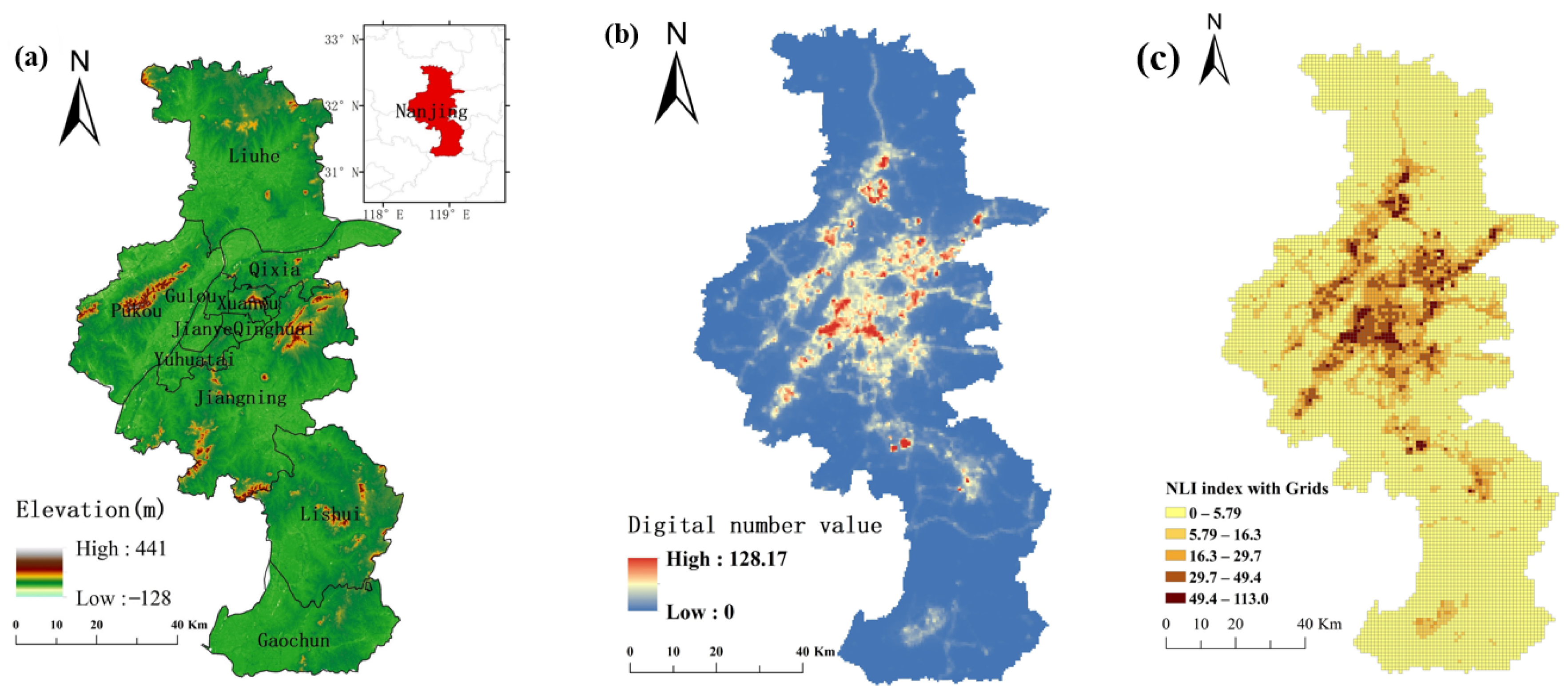
Nanjing is one of the most important cities with a high-level education base and transport hub (Figure 2a). Nanjing includes eleven zones whose total area is 6587 km2, placed in the lower stretches of the Yangtze River Delta. By the end of 2018, there were 8.3 million registered residents; 81% were urban residents. GDP in Nanjing was 960 billion yuan (~140 billion USD), ranking 10th among Chinese cities. Infrastructure enhancement, population development, and economic profitability have resulted in a high request for commercial and living space, gradually developing into the rural regions near the city [30].
Nighttime light data can be used to infer the transitional urban–rural regions’ regional spatial properties, and thereby can be employed as a diagnostic characteristic for detecting urban and rural regions [31,32]. The data used in the analysis were collected in 2018. Night lighting data with a resolution of 1 km in each month of 2018, acquired by the Suomi National Polar-orbiting Partnership (Suomi NPP) satellite, was downloaded from the National Geographic Data Center located at the National Oceanic and Atmospheric Administration web page (https://www.ngdc.noaa.gov/eog/viirs/download_dnb_composites.html (accessed on 7 July 2022).
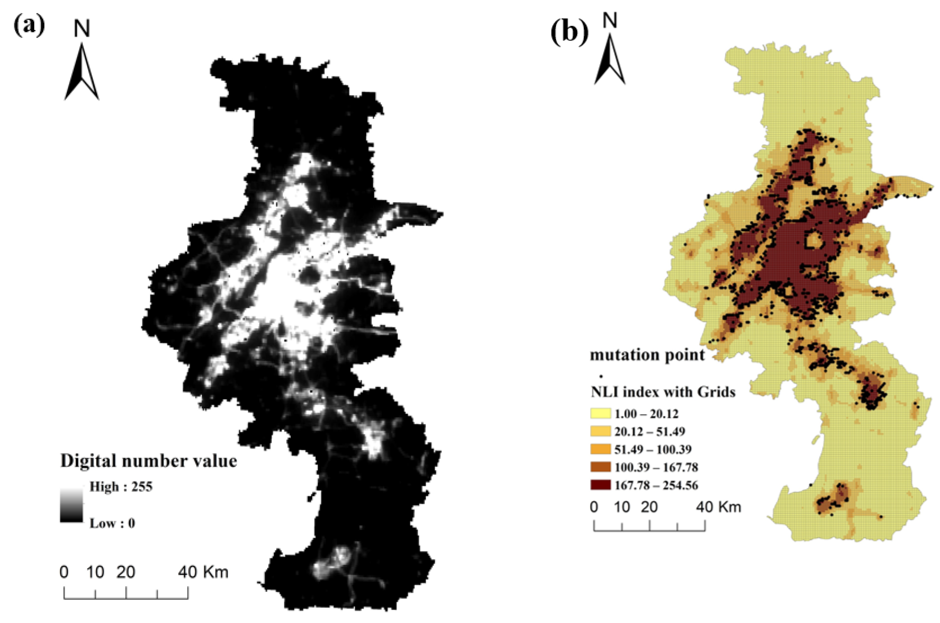
From the city center to the countryside, the nighttime light intensity gradually decreases, with a transition characteristic of ‘smooth–fluctuated–smooth’ [19]. Therefore, the nighttime light intensity (NLI) in the urban fringes can be used to show transitional characteristics from the city to the countryside [31]. NLI is quantified as the digital number (DN) values of pixels from the NPP/VIIRS images (Figure 2b), which can directly reflect the population’s spatial distribution and regional economic activities [33]. The monthly night lighting data were resampled, and the mean intensity of all grid cells was counted as the NLI in 2018. The city epicenters have more significant NLI indices, and the grid units are aggregated. With the increase in the distance from the mentioned centers, the NLI indices decline gently. This converts those pixel parts to discrete parts. Pixels with a bigger NLI index are more grouped than ones having middle-level indexes that generally exist in the urban fringe. The mentioned feature indirectly describes the mutability of the fringe. While considering the methods of identification based on the mutation points in this study, the NLI image data cannot be directly used to recognize urban fringes. We constructed a grid cell of 1 km × 1 km to record the corresponding NLI values of night lighting data that of the original data with 1 km resolution (Figure 2c).

2.2. Mutation Point Detection by SCWT

In the process of urban fringe identification, the abrupt change of nighttime light intensity, as reflected by the mutation points on the grid map of NLI, can be detected by the SCWT method [15]. Mapping the mutation points of a grid map of NLI using SCWT includes three steps. Firstly, transects are extracted from the grid map of NLI; these transects are constructed by line sampling of the grid map of NLI, beginning from the same grid located at the center of the city and ending at each grid located at the edge of the whole map. Secondly, one transect is processed using the SCWT and its wavelet coefficients are calculated, and these points with the wavelet coefficient’s maximum and minimum values are labeled as mutation points. Thirdly, step two is repeated to process all transects.
The grid map of the NLI values will be transected by the model in the first part as 1-D signals, initiating from similar grids (placed in the center of the central urban region) and finishing at all grid cells placed at the map edge for all signals, thus making the map suitable for SCWT. The mutation points of each 1-D signal are then identified and mapped as the map of mutation.
The basic principle underlying the SCWT method involves decomposing the original spatial sequence signal to acquire its approximate and detailed coefficients using wavelet transform. The former reflects the original signals simulations, and the latter reflects the sudden signal changes. The peaks and troughs of the signal changes are called the ‘maximum modulus’ points of the wavelet coefficients and are always considered to be the locations of mutation points.
SCWT a , b = S x φ x = 1 a 0 L x S x φ x b a d x ,
where SCWT a , b represents the wavelet coefficients, S x describes the signal of a spatial sequence (the original one), and φ x denotes a wavelet basic mapping, including a spatial scale ( a ) and shifting proxy ( b ), where the latter is controlled by the unique factor of the wavelet function (scale a ), which determines the decomposition effect.

2.2.1. Selection of Wavelet Basic Function

Before processing the wavelet transform, scholars should obtain the wavelet basic function that extracts a result describing the signal’s considerable impact, which precisely reflects the incoming signal’s feature. Using the SCWT method, two types of mutation points are identified in the spatial sequence signal [34]. The first type corresponds to smooth signals without mutations, with discontinuous and mutated first derivatives (Figure S1). The second type corresponds to signals with sudden amplitude changes at certain positions, which lead to signal discontinuity (Figure S2). In the urban fringe detection process, the sudden variation of NLI values, as reflected by the mutation points on the NLI map, emerges within a distinctly sharp rise. Thus, the mutation points were described by the second kind of discontinuity [15,16,35]. Db3 wavelet was then chosen as the wavelet basic function, acquired from the Daubechies wavelet family employed in the second type of discontinuity identification works in this study (Figure S2).

2.2.2. Determination of Spatial Scale in SCWT

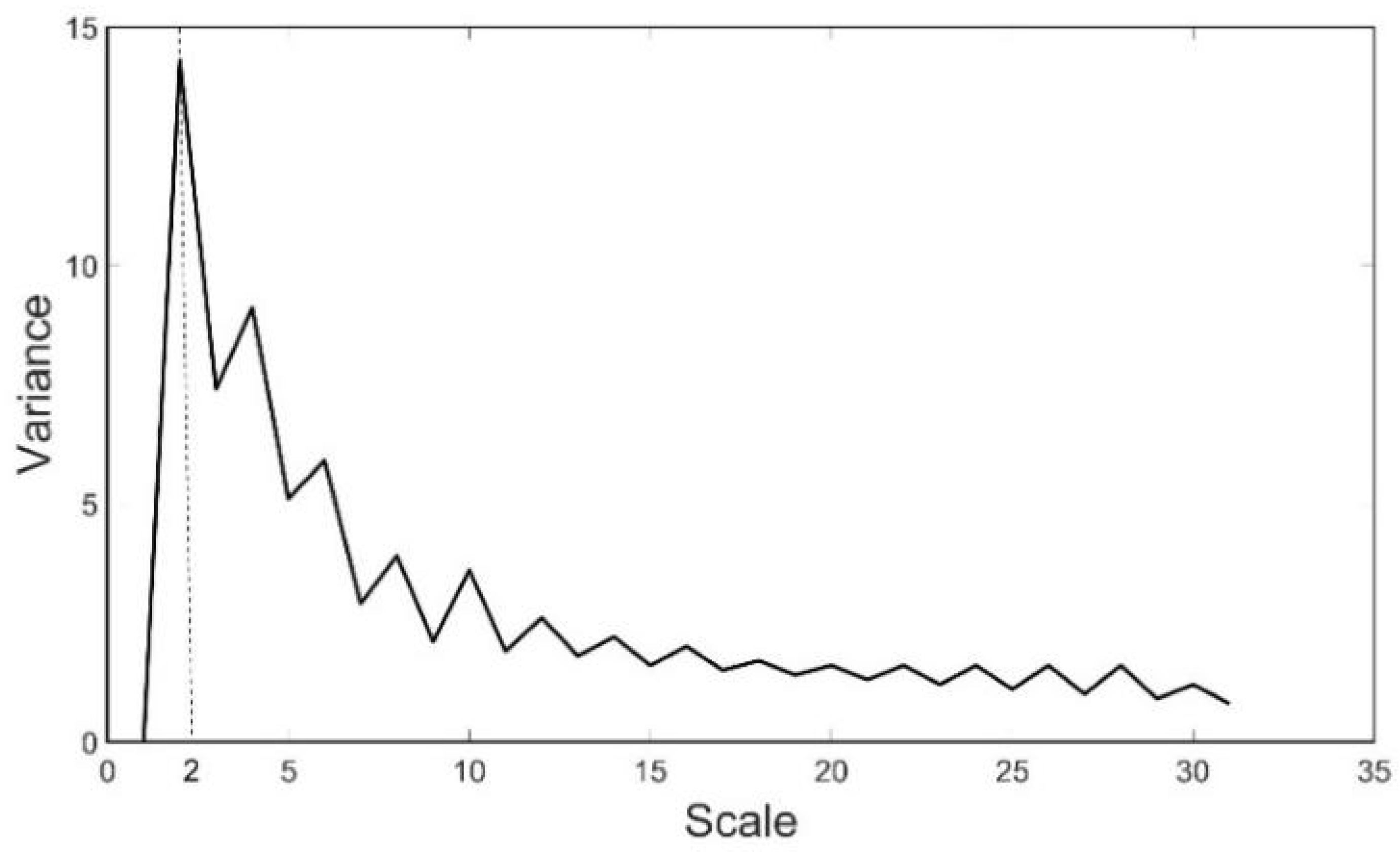
Choosing a proper transformation scale for identifying the mutation points is critical. Notably, many mutation points will be neglected when the scale is large. If the scale is small, the result will contain significant noise. The current work employs a plot of the wavelet coefficients’ variance to choose the scale fitted mostly [36]. As the scale reaches the highest variance value, it achieves a considerable signal impact, which can precisely reflect the incoming signal features. Figure 3 depicts that the curve of obtained variance indicated the second processing scale (i.e., Scale a = 2) had the maximum variance of the coefficients between the scales of the wavelet transform. Thus, the local maximum in the coefficients processed in Scale = 2 is explored by the model as the points of mutation points and eventually mapped all the mentioned regions (of all the transects coefficients) as a map of mutation points.

2.2.3. Elimination of “Pseudo” Mutation Point

Researchers usually label the location of mutation points by recording and mapping the “maximum module” of wavelet transform coefficients. Although the “modulus maximum” of the wavelet transform can correspond to more signal mutations, plenty of noises (i.e., “pseudo” mutation points) may be produced, making it challenging to place the mutation points more precisely [35]. As shown in Figure 4a, the wavelet coefficient curve was obtained by wavelet transform, and the wavelet coefficient’s maximum and minimum values are also calculated and marked. Many sudden urbanization-level variations happen in the urban fringe, indicating a remarkable transition from one stable state to another, characterized by high wavelet coefficient values [19]. Thus, eliminating the “pseudo” mutation point, characterized by low wavelet coefficient values, will attain an accurate urban fringe detection (discussion in Section 4.1).
To delineate the “true” mutation points within the urban fringe, the slicing threshold should derive the urban fringe areas, limited by mutation with high wavelet coefficient values with maximum continuity. The literature on delimitating different city regions generally presents a value of k-standard deviations [37]. Suppose that we have a set consisting of the points of mutation x1, x2, x3, …, xn, where their average   x   ¯ and k standard deviations are described as the following:
x i   x   ¯ > k σ
It is assumed that the wavelet coefficient values of “pseudo” mutation points in the interval of x ± k σ are normal, and the scores of “true” mutation points exceeding the range are abnormal (Figure 4b). The current test employed an appropriate value of two standard deviations.

2.3. Urban Fringes Identification by Dual Spatial Clustering

As discussed above, the urban fringe is a particular area comprising mutation points. A spatially local cluster, including similar neighboring mutation points (satisfying the spatial proximity and attribute similarity specifications), might exist in the urban fringe. To identify this particular cluster, a modified dual spatial clustering derived from the DBSC approach [38] is employed. A two-level distance constraint first established heterogeneous proximity relationships between mutation points in this modified model. Then, attribute information entropy is utilized to develop an adaptive attribute clustering approach for clustering with attribute similarity after establishing spatial proximity relationships.

2.3.1. Construction of Spatial Proximity Relationships

Given the non-uniform size and shape of the boundaries in urban fringes, mutation points are often distributed irregularly. This paper adopts a two-level approach from the DBSC algorithm to construct heterogeneous proximity relationships between mutation points [38]. The first step eliminates lengthy edges at the global level. In contrast, the second step removes lengthy edges at the local level. Mutation points with similar edges are detected as spatial neighborhoods after two trimming steps.
Suppose M D B is the mutation points database, and D T M D B represents the M D B ’s Delaunay triangulation. For every point P M D B , the global edge-length constraint is described as the following:
  G l o b a l L e n g t h _ C o n s t r a i n t P = G l o b a l M e a n D T + α G l o b a l V a r i a t i o n D T
α = G l o b a l M e a n D T / L o c a l M e a n P
where G l o b a l M e a n D T is the average length of the edges in D T M D B ; L o c a l M e a n P denotes the average length of edges directly incident to P ; G l o b a l V a r i a t i o n D T denotes the standard deviation of the length of each edge in D T M D B .
Suppose the length of an edge directly incident to P   is more significant than G l o b a l L e n g t h _ C o n s t r a i n t P . In that case, the edge is eliminated from the D T M D B . Local long edges retain after the global operation. Thus, using the edge length of each parcel centroid in the second-order neighborhood, the following local proximity requirement is defined to remove the residue lengthy edges:
L o c a l L e n g t h _ C o n s t r a i n t P = 2 o r d e r M e a n P + β M e a n V a r i a t i o n P
where 2 o r d e r M e a n P   stands for the average length of each edge belonging to a trajectory of two or smaller edges beginning from P ; M e a n V a r i a t i o n P describes the average of all L o c a l _ V a r i a t i o n Q for mutation point Q belonging to the trajectory of two or smaller edges beginning at P ; L o c a l _ V a r i a t i o n Q stands for the standard deviation of the length of the edges directly incident to Q . When the length of an edge belonging to a second-order neighborhood of P is more significant than L o c a l L e n g t h _ C o n s t r a i n t P , the edge will be deleted from D T M D B . Through the global and local proximity criteria, D T M D B   can be categorized into several sub-graphs by removing ‘inconsistent’ edges to obtain an accurate proximate relationship.

2.3.2. Clustering Mutation Points with Attribute Similarity

The attribute similarity (i.e., NLI index) strategy, the second part of DBSC algorithm, aims at detecting the homogeneous spatially fringe clusters based on the trimming results obtained from DT(MDB). Nevertheless, it is challenging to deal with attribute similarity under the simultaneous occurrence of heterogeneity and noise as the attribute similarity measurement is established using a binary predicate adopting the Euclidean distance. Existing work has found that the attribute similarity measurements designed for the Euclidean situation may cause severe over- or under-segmentation in the identification of spatial point events [39,40].
The current work determines the attribute similarity between mutation points using the information entropy. Information entropy (IE), as a measure of dispersion, uncertainty, disorder, and diversification related to a random variable or its probability distribution, can be employed as an appropriate index to measure the attributes and verify their corresponding distribution [41]. The modified algorithm determines the neighbor entropy for all mutation points and explores the adjacent neighbors having a higher neighbor entropy. According to the mentioned assumptions, the cluster center point inherently contains the maximum neighbor entropy. This means that the cluster center point is at the top of the sequence while calculating and sorting the mutation points’ neighbor entropy. The local similarity among neighboring mutation points and the global similarity between a mutation point and the others can be employed as the IE In the following, the three essential algorithm steps, including the neighbor entropy calculation, obtaining the similarity to the cluster center point, and producing various clusters, are presented.

Neighbor Entropy Computation for Each Mutation Point

The method proposed by Shannon [42] is employed to calculate the attribute IE. Accordingly, the entropy value is higher when the feature score of each point is similar. When the change is significant, the entropy value is smaller. This is attained by proportionating each value in a dataset to its summation of scores as the probability [41], and thereby we use it to determine the attribute IE (Figure S3). Let n be the whole number of mutation points A , the NLI score of A is described by R = r 1 ,   r 2 , , r n . This probability is described as the following:
P k = r k / k = 1 n r k ,   k = 1 , 2 , . , n
where P k denotes the proportion of the NLI value of all mutation points to the sum of all mutation points’ NLI values. Obviously, k = 1 n P k = 1 , which meets the normalization condition; the attribute IE of A is obtained as:
H M r = k = 1 n P k log 2 P k
After obtaining the mentioned attribute IE, the neighborhood entropy H n e a r p   of a mutation point is described as the following: For a mutation point p , all the mutation points of its adjacent neighborhoods, involving itself, are represented by N e i p . The neighborhood entropy of p is defined as
H n e a r p = H n = N e i p M r / N e i p
where H n = N e i p M r describes the IE of N e i p and N e i p represents the number of mutation points in N e i p . Neighborhood entropy determines the resemblance between p and adjacent neighborhoods. The value of H n e a r p is high when the mutation point p is analogous to its adjacent neighborhoods.

Calculating Similarity from the Cluster Center Mutation Point

As discussed above, the mutation point with the maximum neighbor entropy is chosen as the cluster center. By computing   H n e i p   for whole mutation points ranked in inclining order, the center of the cluster center is described by
C l u s t e r _ c e n t r e p 1 = m a x H n e i p
After determining the cluster center, its similarity to the remaining ungrouped mutation points is obtained. They can be divided into a direct neighbor (the first-order neighborhood in the proximate graph) and an indirect neighbor (k-order neighborhood, k > 1) based on the neighbor relationship with the cluster center:
Most previous studies determined the similarity between attributes using the Euclidean distance. Nevertheless, the mentioned similarity index can lead to significant over- or under-segmentation faced with heterogeneity problems. Accordingly, we consider local and global similarity based on IE. Equally,
D i s t x 1   , x 2 = H x 1 x 2 M r         i f   x 1   D N x 2   o r   x 2   D N x 1
D i s t p ,   B = H p B M r             o t h e r w i s e
Equation (9), which represents the local similarity, considers the disparity between the center point of the cluster and its direct neighborhoods; when more points of mutation (greater than 2) are appended to the original cluster, Equation (10), which represents the global similarity, can consider the disparity between the ungrouped points of mutation point and a set of mutated ones, where B is composed of a set of points of mutation, and p describes an ungrouped point of mutation (Figure S4).

Producing Various Clusters

After obtaining the center of the cluster and similarity index, the mutation of points that remained ungrouped is classified starting from the cluster center p 1 . The mutation points belonging to the direct neighbors of p 1 are initially ranked in inclining order according to their corresponding feature IE. The original cluster is constructed if they meet the resemblance criteria (Equation (11)). For all mutation points belonging to the indirect neighbors of p 1 , the initial point to be appended to the first cluster is selected as the starting point, and both direct and indirect neighborhoods are visited in descending order based on their corresponding attribute IE. When no mutation points can be appended to the cluster starting at p 1 , the initial spatial cluster is attained. The cluster center is then reselected through the mentioned operation based on the ungrouped points of mutation, and the above traverse operation can repeatedly group both direct and indirect neighborhoods (Figure S5). The current work ranks the cluster center’s direct and indirect neighborhoods based on their corresponding attribute IE and visited them through the breadth-first search approach [43].
The similarity threshold condition is a critical problem in spatial clustering. The attribute resemblance function is established based on the highest entropy theory. According to Equation (5), the feature IE attains its highest score, and the cluster attains the highest resemblance for a cluster with equal probabilities. When an unclassified mutation point is the same as a known point or cluster, the new cluster’s IE will be high based on the information entropy’s monotonicity. According to the mentioned assumptions, a point q or a cluster C is similar to a mutation point p if the following condition is fulfilled:
H M / H m a x M θ
where   H M   represents a new cluster’s information entropy, including p , q   o r p ,   C , and H m a x M   denotes the new cluster’s maximum IE. H M / H m a x M represents the normalized entropy of the feature n o r m H M r . Therefore, a middle score for the parameter, 0 < θ < 1 , accommodates a distinct clustering interval.
The similarity parameter θ adjusts the local spatial difference’s sensitivity, which is challenging to acquire without enough previous knowledge. The current work employs a cluster assessment measure, the PBM index, to attain good results by adjusting an appropriate value of θ . From [44], the PBM index outperforms in both modes, which is crisp and fuzzy, as local spatial patterns in clustering. The calculation formula is defined by
  PBM = 1 N c E 1 E N c D N c 2
E N c = i = 1 N c E i ,   E i = j = 1 N i x j v i , D N C = m a x i , j = 1 N C v i v j
where   N c   represents the cluster numbers,   N i   describes the entire points in the cluster C i ,   v i stands for the center of the cluster C i   , and D N c determines the highest distinction between a pair of clusters. When the index called PBM attains its highest score, the best segmentation can be attained. Hence, the law of IE measurement is an acceptable result.

Implementation Procedure of the Algorithm

The algorithm is run utilizing 3 steps.
Step 1. Establish the spatial proximity relationships between the mutation point set. The following operation should be performed to implement this step:
Establish the DT for the mentioned mutation points.
Eliminate the edges from the DT based on the global edge-length constraint.
Eliminate the edges from the DT according to local edge-length constraints.
Step 2. Compute the neighbor entropy. For each mutation point, calculate its neighbor entropy and sort the mutation point set in descending order by neighbor entropy.
Step 3. Implement attribute clustering. This step involves the following operations:
Choose the highest neighbor entropy as   C l u s t r e _ P o i n t p .
Utilize the BFS to visit both direct and indirect neighborhoods of p in the inclining order of their corresponding neighbor entropy. The cluster is constructed when they meet Equation (11), and no new mutation point is appended to the cluster, thereby detecting them as clustered.
Traverse all mutation points that are not clustered by iterative operations ①–②. When clustering is finished, any mutation point that does not belong to a cluster will be identified as noise.
The implementation procedure of attribute clustering is further illustrated. Figure 5 depicts the simulation of the data. The NLI scores for the points of mutation are tagged in Figure 5a. All mutation points’ neighborhood entropy is first calculated. P1 is chosen as the initial point of the clustering center (Figure 5b), and its neighborhoods are identified as the initial cluster C1 ( θ   = 0.985). P2 is then detected as the new point of the clustering center, and its neighborhoods construct C2 called the second cluster. In the end, P3 is picked as the center point of the clustering, and its neighborhoods are grouped as C3. The clustering outcomes of the simulated datasets (Figure 5b) indicate that points in a similar are the same as both the spatial and feature domains. Figure 5c presents the obtained curve graph, where the x-axis and y-axis indicate the θ value and the PBM index, respectively. The highest PBM index is attained for θ = 0.985. Notably, the index of PBM varies when θ = 0.90; this variation happens because spatial proximity and attribute similarity clustering results are considered similar in the range (0, 0.90].

2.4. Boundary Derivation of the Mutation Point Set

The dual spatial clustering approach was employed to attain various mutation point sets connected through the DT. A Delaunay-based shape reconstruction presented by Peethambaran and Muthuganapathy [45] is employed to precisely detect the boundaries. The urban fringe comprises outer and inner boundaries to construct a hollow shape geometrically. The benefit of the mentioned method is that both cavities and holes in the form of planar points can be identified, making it applicable to detect fringe boundaries. The boundary points’ Delaunay triangulation was initially constructed for the point set. Next, the triangle filtration proceeded by repeatedly eliminating thin boundary triangles while meeting the CIRCUMCENTER and REGULARITY requirements (More information on triangle filtration can be found in [45]).

3. Results

3.1. Mutation Point Detection

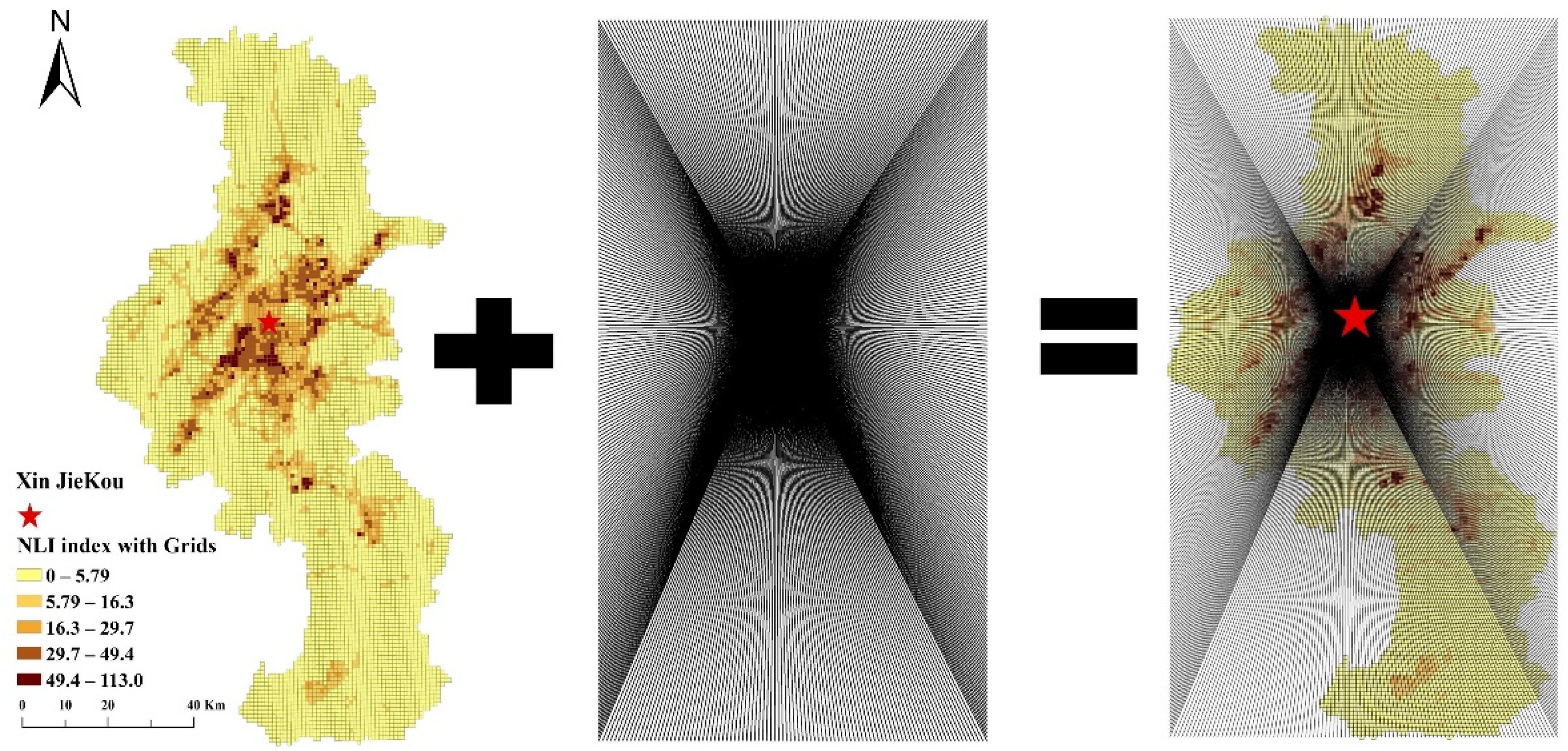
A downward inclination is exhibited regarding the light intensity of the nighttime in Nanjing City between the city center through the surrounding regions. To make the NLI value map applicable for SCWT, a city center was utilized as the beginning point, and 360 sampling lines were attained using a one-degree range [15]. The current work derived the sample lines by setting Xinjiekou, the primary center (indicated in Figure 6) of Nanjing, as the start location. The outermost grid center of the study region was chosen as the final point. Overall, 554 sample lines were acquired for the city center.
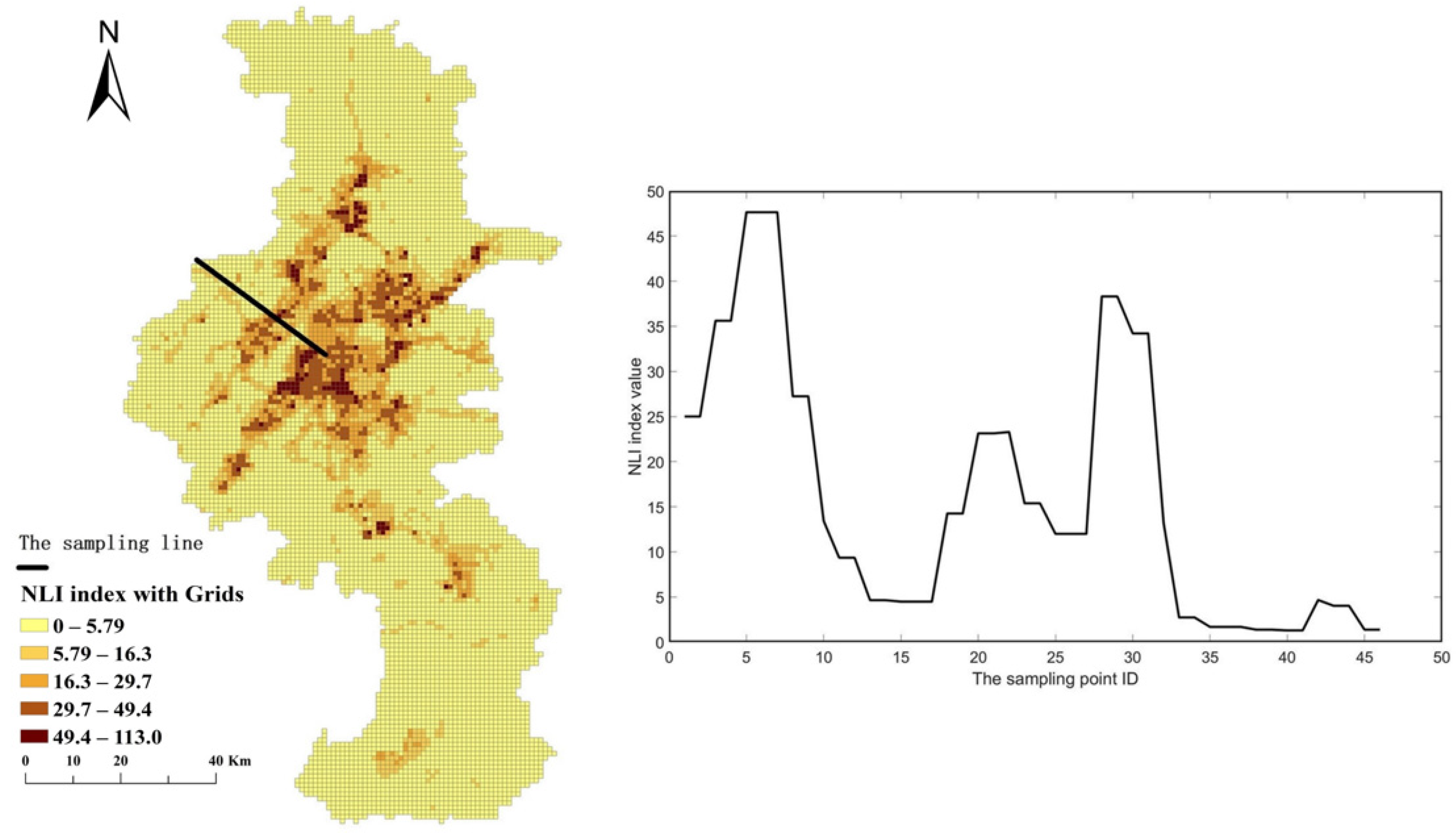
Each sample line’s spatial sequence signal was established by registering the NLI indices of the grids crossing the sample line from the city center to the periphery. The sample line exhibits an apparent urban–rural transition (Figure 7), where the NLI values changed along with the sample line on the map of NLI. The various features of nighttime light crossing the urban fringe region and the outer rural region were described. The sample points with IDs of 1–7 and 18–33, near the city center and located in growth zones, respectively, are in the urbanization–growth step. In the mentioned regions, the utilization types of both urban and rural lands are combined and have a random mosaic structure, leading to the urban infrastructure distributed nonuniformly infrastructure in which lights of nighttime alter. All are related to regional features of urban fringes. The sample points having IDs between 34–46, far away from the center of the city, are less urbanized and include inadequate urban infrastructure, exhibiting low nighttime light, compatible with standard features of rural areas.
Then, each signal’s mutation points (its highest and smallest scores) are detected through the approach called SCWT with the optimum scale (i.e., Scale a = 2) and wavelet basic function processed by db1 in Section 2.2.2. After mapping the points of mutation identified utilizing the entire as points, the model further eliminates “pseudo” mutation points using two standard deviation values. Ultimately, 473 mutation points were identified in the center with many intersection points (Figure 8).

3.2. Urban Fringe Identification

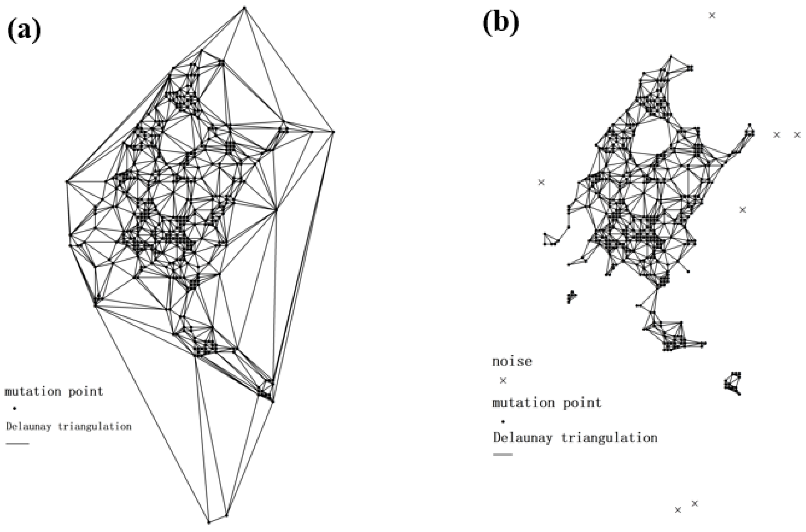
In the first step, Delaunay triangulation is presented to establish spatial proximity between the mentioned detected mutation points in Section 3.1, and their neighbor relations are described with edges as linking pairs of points. It can be observed that the detected mutation points are dispersed unevenly while covering the whole city densely. A spatial data distributed irregularly has imperfect natural neighborhoods distinguished through DT with varying densities. DT containing edge-length requirements globally and local constraints is further adopted to describe the spatial heterogeneous proximity correspondences between the mentioned points (Figure 9). It means employing large and small search radii for low-density and high-density regions, respectively. Therefore, every node and edge can store the required data for running the model, such as neighboring mutation points and NLI values.
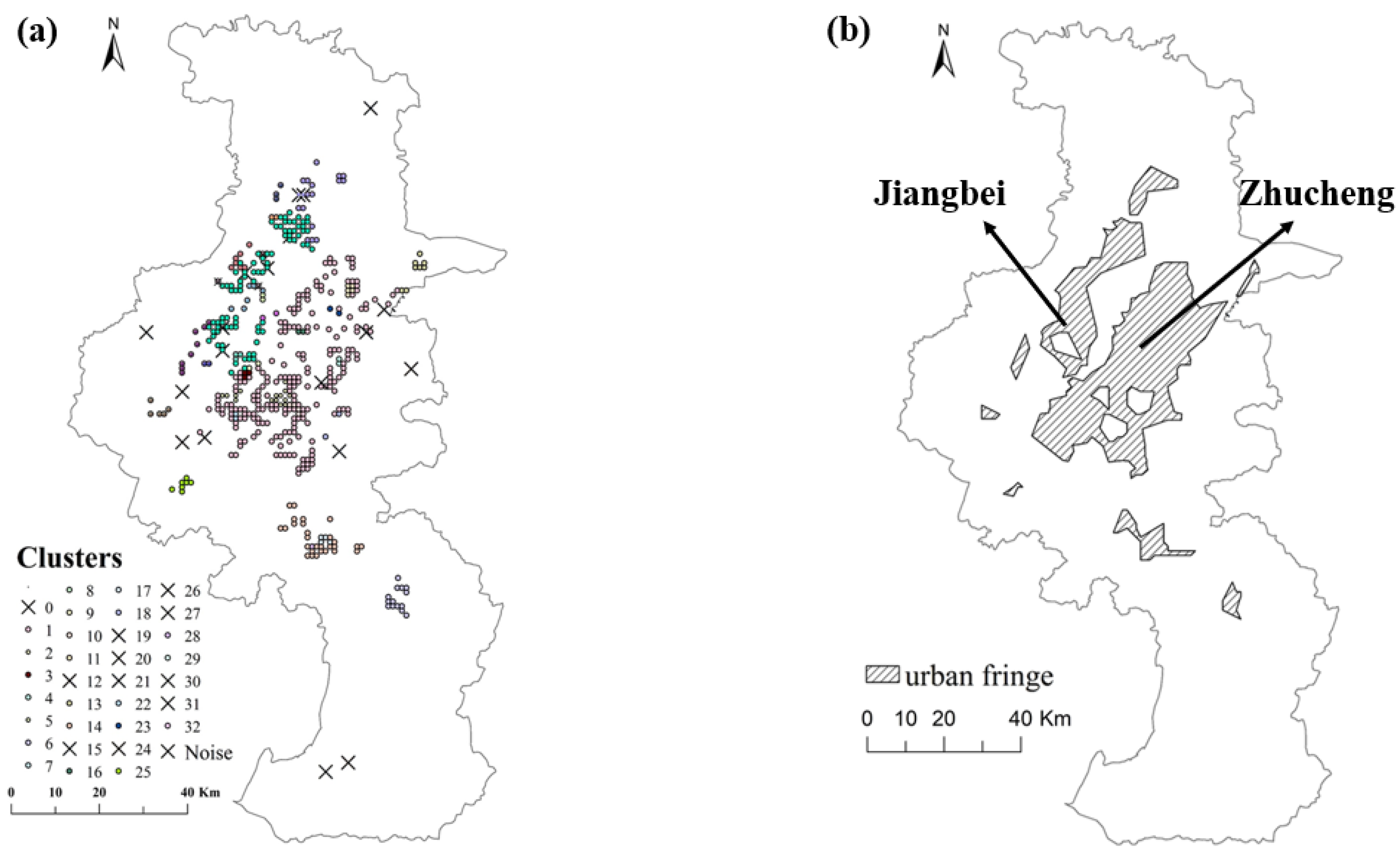
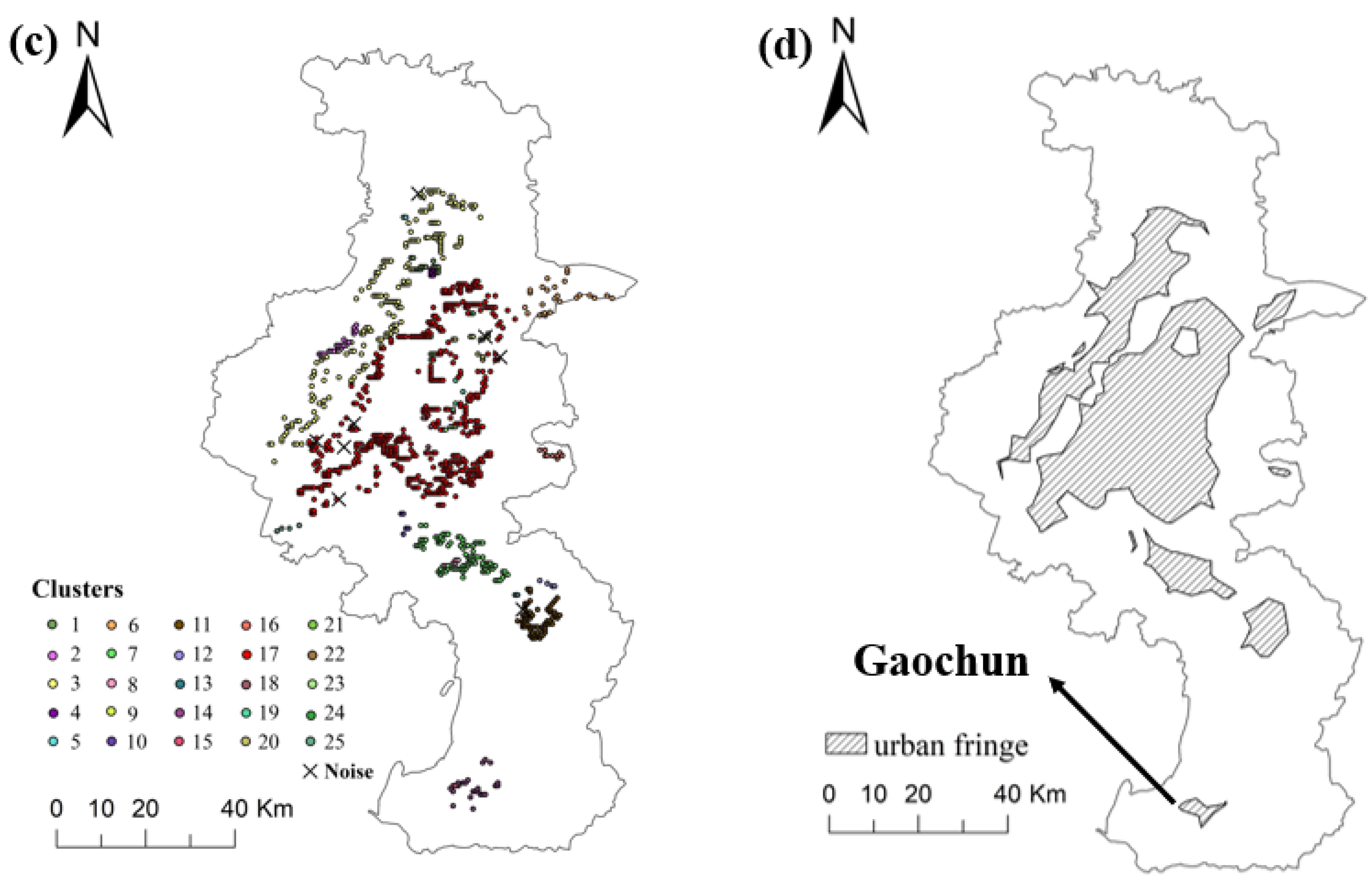
After performing the global and local trimming, the information entropy-based attribute clustering approach is applied to the NLI index of mutation points. As shown in Figure 10a, the points with similar colors lie in similar clusters, and the points described with “x” are identified as noise whose spatial location and attribute values significantly differ from those of other mutation points in its spatial neighborhood, where 22 main clusters are discovered. The basic statistical information of these clusters is listed in Table 1. We can see that there is a significant difference between adjacent clusters, and that the variation in each cluster is small. This information can reflect different urbanization levels characterized by NLI in this region. The boundary of the urban fringe is identified by linking the most adjacent mutation points, taking into account both spatial proximity and attribute similarity. The urban fringe is a combination of the outer and inner boundaries. We implement a density-based algorithm in Section 2.4 to identify the boundaries, which can detect both cavities and holes in planar points. The clustering results of our algorithm are shown in Figure 10b. Moving from north to south of Nanjing, the two main urban fringe segments are Jiangbei and Zhucheng, suggesting that human activities occurring at night are concentrated in these two regions.

4. Discussion

4.1. The Influence of Using the Strategy of Eliminating “Pseudo” Mutation Points

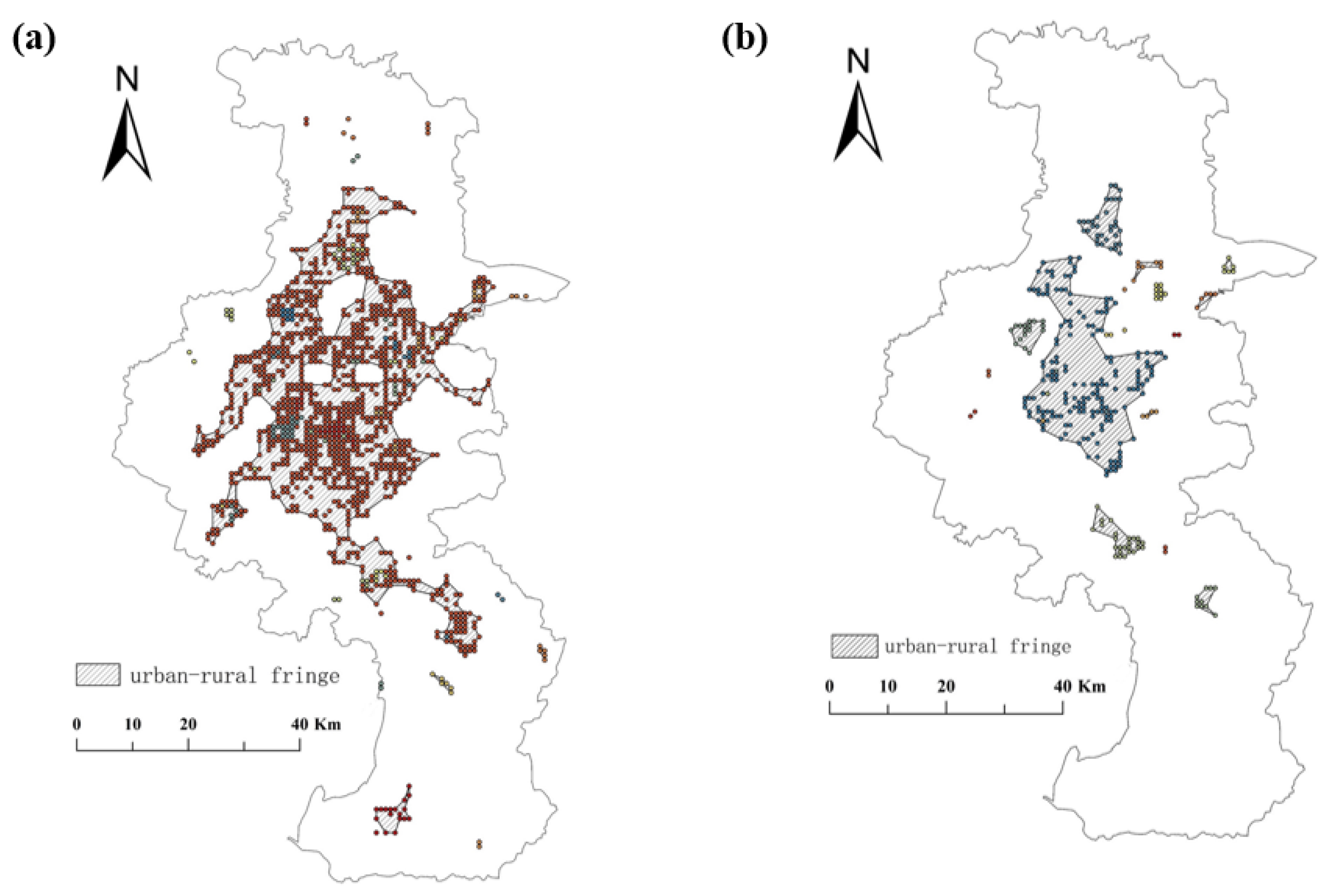
To further prove that the strategy of eliminating “pseudo” mutation points can lead to a more accurate result for identifying urban fringes, here, we extracted urban fringes with different slicing thresholds (k = 0. k =2.0, and k =3.0) in Equation (2) and compared the extracted results with the above-identified results. Figure 11a,b display the influence of different slicing thresholds on the mutation points pattern (the points with similar colors lie in similar clusters) and their geographical extents of urban fringes. Generally, no identified mutation point will be removed with k = 0, whereas the local similarity measurement promotes more neighbors on denser points to integrate a larger cluster, covering a broader urban fringe region (Figure 11a). As the k value increases from 0 to 2.0, the strategy starts to filter the body of mutation points pattern, the clusters with different densities are detected, and the NLI attribute values of these points are significantly different from those of other points in the clusters with k = 2.0 (Figure 10a). As the k value increases from 2.0 to 3.0, the distribution of mutation points is sparse and scattered and more mutation points will be removed since a larger k value can eliminate more points. As shown in Figure 11b, only a few clusters covering small areas are detected, excluding some interesting areas with k = 3.0. Hence, it is reasonable and feasible to study the urban fringes with k = 2 in this study.

4.2. Comparison of Identified Regions Using Different Dual Spatial Clustering

Three typical dual spatial strategies, including modified k-means (Mk-means) [46] and DBSC [38], are also presented for comparison goals. Moreover, the k-means approach takes into account both spatial and non-spatial features, the distance between points in K-Means can be modified according to Equation (14):
D p i , p j = w 1 D S p i , p j + w 2 D A p i , p j
where D p i , p j is the weighted sum of the normalized spatial distance D S p i , p j and non-spatial distance D A p i , p j between p i and p j . The weights, w 1 and w 2 , are set to 0.5 by default [46].
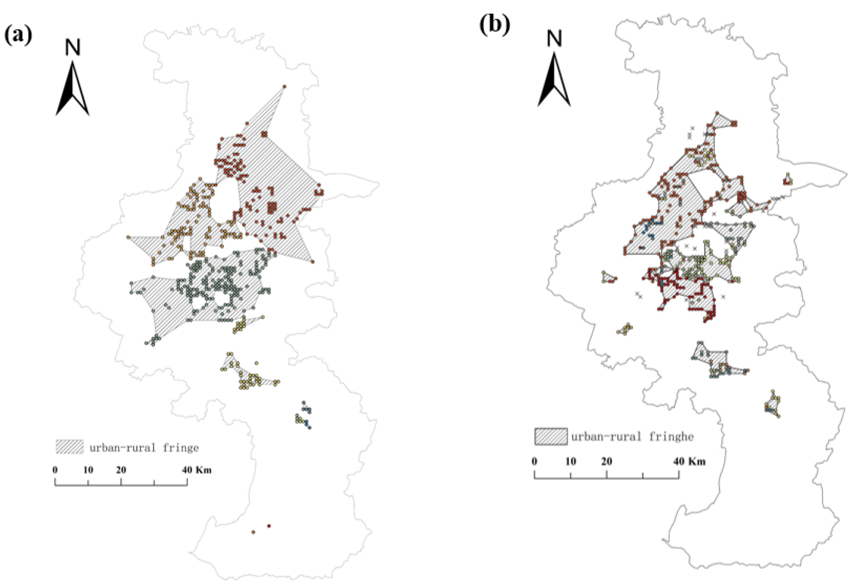
Figure 12 presents the Mk-means and DBSC clustering results, and the points with similar colors lie in similar clusters. Table 2 lists the clusters’ statistical information. The proposed method provides a significant disparity between neighborhood clusters with a generally low standard deviation within all clusters is concluded. The NLI index is an excellent index of various contamination levels. There exist two indispensable fringe partitions related to urban fringes (i.e., Jiangbei and Zhucheng) from north to south Nanjing, indicating that supplemental human exertions at night are focused in the mentioned areas. A significant fringe partition related to the urban fringe appeared from north to south of Nanjing (Figure 10b) and is incompatible with the actual status due to slight disparities between local points of mutation. In other words, the outcome indicates that the DBSC method is inappropriate for nonuniformly distributed features of datasets, where fringes of urban fringe are over-partitioned into various small segments (Figure 12b). Since the noises are not considered in the MK-Means algorithm, specific neighborhood spatial clusters with various features could not be identified (Figure 12a).
Both NLF and RS are employed to evaluate the clustering identification strategies numerically. The bigger the NLF is, the higher the dispersion of the population is, reflecting that the area is more likely to be the urban fringe [31]. RS can determine the constructed clusters’ homogeneity and difference. When the value of RS is zero (0), there is no difference between clusters. Moreover, if RS is 1, there is a remarkable difference between clusters [47]. Table 3 presents a similar variation tendency by two indices with various clustering approaches. The NLF and RS of urban fringe derived through the presented approach are higher than that by the contrast approaches.

4.3. Comparison of Identified Regions Using Different VIIRS Nighttime Light Data

The latest VIIRS dataset is the NASA’s Black Marble product suite. This product provides cloud-free, atmospheric-, terrain-, vegetation-, snow-, lunar-, and stray-light-corrected radiances, which can more accurately reflect human activities [48,49,50]. The all-angle snow-free layer in the Black Marble’s annual moonlight-adjusted nighttime light product (VNP46A4) is used to validate our method. The data preprocessing in the year 2018 has been carried out according to Zheng’s work (https://github.com/qmzheng09work/NTL-VIIRS-BlackMarbleProduct (accessed on 2 September 2022) (Figure 13a). Comparing the two results (Figure 10b and Figure 13d) shows that the overall patterns are similar, and it was initially demonstrated that our method can have a certain degree of reliability using different VIIRS nighttime light data. For example, the two main urban–rural fringe segments, Jiangbei and Zhucheng, are both recognized. However, several details differed. First, the spatial distribution of mutation points deriving from the Black Marble product (Figure 13b) presents an obvious hierarchical structure instead of the concentration state in Figure 8. More specifically, the inner layer of mutation points is ring-shaped, and they are mainly distributed in an area with high light intensity, but affected by terrain. The outer layer of mutation points has a circular structure with low nighttime light intensity, distributed along the edge of the central city. Second, the urban–rural fringes identified by Black Marble data have a larger area compared with that identified by NPP/VIIRS data. The reason for this is that the change in regional spatial patterns between satellite cities and the central city can be characterized by our method. Gaochun, as the district center, has higher urbanization with adequate population density and developed urban infrastructure, and has obvious characteristics of the urban fringe. In this case, Gaochun has been accurately recognized as the urban area and urban fringe using Black Marble data (Figure 13d). To sum up, the proposed recognition method with Black Marble nighttime light data is an effective way to distinguish between the urban fringe and towns and improve the precision and accuracy of the outer boundaries of the fringe range.

5. Conclusions

The current work developed a novel model for detecting the urban fringe by integrating SCWT and dual spatial clustering, which was evaluated by Nanjing City, China, as a case study through NPP/VIIRS nighttime light data. The model precisely identified the mutation of NLI change and mapped it using the mutation points’ SCWT-based identification and mapping. The urban fringe of Nanjing City was detected objectively by slicing the mutation map using the strategy of eliminating “pseudo” mutation points, reflecting a considerable enhancement over the traditional SCWT method without filtering mutation points. By using dual spatial clustering in the urban fringe identification, it transfers the mutation points’ spatial patterns to the homogeneous spatially adjacent clusters effectively, which measures the resemblance between mutation points regarding spatial proximity and attribute similarity. We modified the existing dual spatial clustering to detect clusters under heterogeneity and noise to detect the urban fringe region through the mutation points’ local spatial pattern.
Moreover, detecting fringe regions of urban via the model in Nanjing City was evaluated by running a comparison with conventional spatial clustering methods. The presented approach shows a significant difference between neighborhood clusters and all clusters that have a low SD. By utilizing the information entropy clustering approach, the proposed approach achieves proper inseparable clusters and prevents the over- and under-partition phenomena caused by other methods. Both NLF and RS indices of the urban fringe derived from the presented approach are higher than different approaches. Finally, the established model can detect the urban fringe accurately through NASA’s Black Marble product suite as a comparison case, which can distinguish between the urban fringe and towns and improve the precision and accuracy of the outer boundaries of the fringe range.
There are still various enhancements in the presented approach. The urban fringe is specified by great heterogeneity in spatial urbanization. Urbanization could be specified further precisely through an exhaustive index and multi-source data. Recent studies have established universal urbanization measures with multiple parameters and useful urbanization indicators. They modified the description of spatial urbanization frameworks to promote detection precision. There exist two kinds of cities: mono- and poly-centric. The spatial clustering approach can be employed to identify the urban fringe based on monocentric cities’ mutation point patterns [35]. Nevertheless, its application to the cities of polycentric type, with a spatial polycentric framework of ‘Main center–Subcenter,’ is doubtful.

Supplementary Materials

The following supporting information can be downloaded at: https://www.mdpi.com/article/10.3390/rs14236126/s1.

Author Contributions

J.Z. (Jie Zhu) and J.Y. conceived and designed the experiments; J.Z. (Jie Zhu) and Z.L. performed the experiments and wrote the paper; J.Z. (Jiazhu Zheng) and J.N. analyzed the data; J.N. and M.W. contributed to discussions and validation. All authors have read and agreed to the published version of the manuscript.

Funding

This research was funded by the National Natural Science Foundation of China (Grant No. 42101430), the Ministry of education of Humanities and Social Science project (Grant No.22YJCZH130), the Foundation of Anhui Province Key Laboratory of Physical Geographic Environment (Grant No. 2022PGE006) and the Foundation of Key Lab of Virtual Geographic Environment (Nanjing Normal University), Ministry of Education (Grant No. 2021VGE03, No. 2020VGE04).

Data Availability Statement

The data that support the findings of this study are available from the website given in the manuscript at https://www.ngdc.noaa.gov/eog/viirs/download_dnb_composites.html (accessed on 7 July 2022) and https://blackmarble.gsfc.nasa.gov/#product (accessed on 2 September 2022).

Conflicts of Interest

The authors declare no conflict of interest.

References

  1. Liu, X.; Huang, Y.; Xu, X.; Li, X.; Li, X.; Ciais, P.; Lin, P.; Gong, K.; Ziegler, A.D.; Chen, A.; et al. High-spatiotemporal-resolution mapping of global urban change from 1985 to 2015. Nat. Sustain. 2020, 3, 564–570. [Google Scholar] [CrossRef]
  2. United Nations. World Urbanization Prospects: The 2018 Revision; United Nations 717 Department of Economic and Social Affairs: New York, NY, USA, 2018. [Google Scholar]
  3. Pryor, R.J. Defining the rural-urban fringe. Soc. Forces. 1968, 47, 202–215. [Google Scholar] [CrossRef]
  4. Vizzari, M.; Sigura, M. Landscape sequences along the urban-rural-natural gradient: A novel geospatial approach for identification and analysis. Landsc. Urban. Plan. 2015, 140, 42–55. [Google Scholar] [CrossRef]
  5. Smith, T.L. The Population of Louisiana: Its Composition and Changes; Louisiana State University and Agricultural and Mechanical College, Agricultural Experiment Station: Baton Rouge, LA, USA, 1937; p. 261. [Google Scholar]
  6. Bryant, C.; Charvet, J.P. The peri-urban zone: The structure and dynamics of a strategic component of metropolitan regions. Can. J. Reg. Sci. 2003, 26, 231–239. [Google Scholar]
  7. Antrop, M. Landscape change and the urbanization process in Europe. Landsc. Urban. Plan. 2004, 67, 9–26. [Google Scholar] [CrossRef]
  8. Sharp, J.S.; Clark, J.K. Between the country and the concrete: Rediscovering the rural-urban fringe. City Community 2008, 7, 61–79. [Google Scholar] [CrossRef]
  9. Cao, G.; Liu, T.; Liu, H.; Miao, Y. Changing spatial and structural patterns of non–agricultural activities in outward–moving Beijing urban–rural fringe. Chin. Geogr. Sci. 2012, 22, 718–729. [Google Scholar] [CrossRef]
  10. Masek, J.G.; Lindsay, F.E.; Goward, S.N. Dynamics of urban growth in the Washington DC metropolitan area, 1973–1996, from Landsat observations. Int. J. Remote Sens. 2000, 21, 3473–3486. [Google Scholar] [CrossRef]
  11. Wang, X.; Li, X.; Feng, Z.; Fang, Y. Methods on defining the urban fringe area of Beijing. In Proceedings of the International Symposium on Digital Earth International Society for Optics and Photonics, Beijing, China, 3 November 2010; Volume 7840. [Google Scholar]
  12. Chen, B. Review on identification method and driving mechanism of Peri-urban Area. Prog. Geogr. 2012, 31, 210–220. [Google Scholar]
  13. Zhang, W.; Fang, X.; Zhang, L. Method to identify the urban-rural fringe by TM images. J. Remote Sens. 1999, 3, 199–202. (In Chinese) [Google Scholar]
  14. Qian, J.; Zhou, Y.; Yang, X. Confirmation of urban fringe area based on remote sensing and message entropy:a case study of Jingzhou, Hubei Province. Resour. Environ. 2007, 16, 451–455. (In Chinese) [Google Scholar]
  15. Peng, J.; Zhao, S.; Liu, Y.; Tian, L. Identifying the urban–rural fringe using wavelet transform and kernel density estimation: A case study in beijing city, China. Environ. Model. Softw. 2016, 83, 286–302. [Google Scholar] [CrossRef]
  16. Peng, J.; Hu, Y.; Liu, Y.; Ma, J.; Zhao, S. A new approach for urban–rural fringe identification: Integrating impervious surface area and spatial continuous wavelet transform. Landsc. Urban. Plan. 2018, 175, 72–79. [Google Scholar] [CrossRef]
  17. Dong, Q.; Qu, S.; Qin, J.; Yi, D.; Liu, Y.; Zhang, J. A Method to Identify Urban Fringe Area Based on the Industry Density of POI. ISPRS Int. J. Geo-Inf. 2022, 11, 128. [Google Scholar] [CrossRef]
  18. Gao, Y.; Feng, Z.; Wang, Y.; Liu, J.; Li, S.; Zhu, Y. Clustering urban multifunctional landscapes using the self–organizing feature map neural network model. J. Urban. Plan. Dev. 2014, 140, 11. [Google Scholar] [CrossRef]
  19. Zhao, F.A.; Jian, P.B.; Jwa, B. Using DMSP/OLS nighttime light data and K–means method to identify urban–rural fringe of megacities. Habitat. Int. 2020, 103, 102227. [Google Scholar]
  20. Goodchild, M.F. The validity and usefulness of laws in geographic information science and geography. Ann. Assoc. Am. Geographers. 2004, 94, 300–303. [Google Scholar] [CrossRef] [Green Version]
  21. Zhu, J.; Zheng, J.; Di, S.; Wang, S.; Yang, J. A dual spatial clustering method in the presence of heterogeneity and noise. Transactions 2020, 24, 1799–1826. [Google Scholar] [CrossRef]
  22. Imhoff, M.L.; Lawrence, W.T.; Stutzer, D.C.; Elvidge, C.D. A technique for using composite DMSP/OLS “city lights” satellite data to map urban area. Remote Sens. Environ. 1997, 61, 361–370. [Google Scholar] [CrossRef]
  23. Rom´an, M.O.; Wang, Z.; Sun, Q.; Kalb, V.; Miller, S.D.; Molthan, A.; Masuoka, E.J. NASA’s Black Marble nighttime lights product suite. Remote Sens. Environ. 2018, 210, 113–143. [Google Scholar] [CrossRef]
  24. Li, X.; Zhao, L.; Li, D.; Xu, H. Mapping urban extent using Luojia 1–01 nighttime light imagery. Sensors 2018, 18, 3665. [Google Scholar] [CrossRef] [PubMed] [Green Version]
  25. Zheng, Q.; Weng, Q.; Huang, L.; Wang, K.; Deng, J.; Jiang, R.; Gan, M. A new source of multi-spectral high spatial resolution night-time light imagery—JL1-3B. Remote Sens. Environ. 2018, 215, 300–312. [Google Scholar] [CrossRef]
  26. Guo, W.; Lu, D.; Wu, Y.; Zhang, J. Mapping impervious surface distribution with integration of SNNP VIIRS-DNB and MODIS NDVI data. Remote Sens. 2015, 7, 12459–12477. [Google Scholar] [CrossRef] [Green Version]
  27. Zhou, Y.; Li, X.; Asrar, G.R.; Smith, S.J.; Imhoff, M. A global record of annual urban dynamics (1992–2013) from nighttime lights. Remote Sens. Environ. 2018, 219, 206–220. [Google Scholar] [CrossRef]
  28. Omar, A.H.; Winker, D.M.; Tackett, J.L.; Giles, D.M.; Kar, J.; Liu, Z.; Vaughan, M.A.; Powell, K.A.; Trepte, C.R. CALIOP and AERONET aerosol optical depth comparisons: One size fits none. J. Geophys. Res. Atmos. 2013, 118, 4748–4766. [Google Scholar] [CrossRef]
  29. Román, M.O.; Stokes, E.C. Holidays in lights: Tracking cultural patterns in demand for energy services. Earth’s Futur. 2015, 3, 182–205. [Google Scholar] [CrossRef]
  30. Gao, C.; Feng, Y.; Tong, X.; Lei, Z.K.; Chen, S.R.; Zhai, S.T. Modeling urban growth using spatially heterogeneous cellular automata models: Comparison of spatial lag, spatial error and GWR. Comput. Enviro. Urban. 2020, 81, 101459. [Google Scholar] [CrossRef]
  31. Yang, Y.; Ma, M.; Tan, C.; Li, W. Spatial Recognition of the Urban-Rural Fringe of Beijing Using DMSP/OLS Nighttime Light Data. Remote Sens. 2017, 9, 114. [Google Scholar] [CrossRef] [Green Version]
  32. Chen, X.; Jia, X.; Pickering, M. Urban-Rural Fringe Recognition with the Integration of Optical and Nighttime Lights Data. In Proceedings of the IGARSS 2019—2019 IEEE International Geoscience and Remote Sensing Symposium, Yokohama, Japan, 28 July 2019–2 August 2019. [Google Scholar]
  33. Cai, J.; Huang, B.; Song, Y. Using multi-source geospatial big data to identify the structure of polycentric cities. Remote Sens. Enviro. 2017, 202, 210–221. [Google Scholar] [CrossRef]
  34. Fagan, W.F.; Fortin, M.J.; Soykan, C. Integrating edge detection and dynamic modeling in quantitative analyses of ecological boundaries. BioScience 2003, 53, 730–738. [Google Scholar] [CrossRef] [Green Version]
  35. Yang, J.; Dong, J.; Sun, Y.; Zhu, J.; Huang, Y.; Yang, S. A constraint-based approach for identifying the urban–rural fringe of polycentric cities using multi-sourced data. Int. J. Geogr. Sci. 2021, 36, 114–136. [Google Scholar] [CrossRef]
  36. Mallet, S. A Wavelet Tour of Signal Processing: The Sparse Way, 3rd ed.; Academic Press: New York, NY, USA, 2008. [Google Scholar]
  37. Yu, W.; Ai, T.; Shao, S. The analysis and delimitation of Central Business District using network kernel density estimation. J. Transp. Geogr. 2015, 45, 32–47. [Google Scholar] [CrossRef]
  38. Liu, Q.L.; Deng, M.; Shi, Y.; Wang, J.Q. A density-based spatial clustering algorithm considering both spatial proximity and attribute similarity. Comput. Geosci. 2012, 46, 296–309. [Google Scholar] [CrossRef]
  39. Zhu, J.; Sun, Y.; Li, J. Spatial clustering method considering spatial distribution feature in the attribute domain. J. Remote Sens. 2017, 21, 917–927. [Google Scholar]
  40. Zhu, J.; Sun, Y.Z.; Chen, L.Y.; Zhou, W.; Meng, Y.W. A Spatial Clustering Method Based on Uneven Distribution of Non-spatial Attributes-Identifying City Commercial Center. Geomat. Inf. Sci. Wuhan Univ. 2017, 42, 1696–1702. [Google Scholar]
  41. Li, Z.L.; Huang, P.Z. Quantitative measures for spatial information of maps. Int. J. Geogr. Inf. Sci. 2002, 16, 699–709. [Google Scholar] [CrossRef]
  42. Shannon, C.E. A mathematical theory of communication. Bell Syst. Tech. 1948, 27, 379–423. [Google Scholar] [CrossRef]
  43. Cormen, T.H.; Leiserson, C.E.; Rivest, R.L. Introduction to Algorithms; MIT Press: Cambridge, MA, USA, 1990. [Google Scholar]
  44. Pakhira, M.K.; Bandyopadhyay, S.; Maulik, U. Validity index for crisp and fuzzy clusters. Pattern Recognit. 2004, 37, 487–501. [Google Scholar] [CrossRef]
  45. Peethambaran, J.; Muthuganapathy, R. A non-parametric approach to shape reconstruction from planar point sets through Delaunay filtering. Comput. Aided Des. 2015, 62, 164–175. [Google Scholar] [CrossRef]
  46. Lin, C.R.; Liu, K.H.; Chen, M.-S. Dual clustering: Integrating data clustering over optimization and constraint domains. IEEE. T Knowl. Data. Eng. 2005, 17, 628–637. [Google Scholar]
  47. Halkidi, M.; Batistakis, Y.; Vazirgiannis, M. Clustering validity checking methods: Part II. ACM Sigmod Rec. 2002, 31, 19–27. [Google Scholar] [CrossRef]
  48. Zhu, C.; Li, X.; Ru, Y. Assessment of Socioeconomic Dynamics and Electrification Progress in Tanzania Using VIIRS Nighttime Light Images. Remote Sens. 2022, 14, 4240. [Google Scholar] [CrossRef]
  49. Zheng, Q.; Weng, Q.; Zhou, Y.; Dong, B. Impact of temporal compositing on nighttime light data and its applications. Remote Sens. Environ. 2022, 274, 113016. [Google Scholar] [CrossRef]
  50. Li, T.; Zhu, Z.; Wang, Z.; Román, M.O.; Kalb, V.L.; Zhao, Y. Continuous monitoring of nighttime light changes based on daily NASA’s Black Marble product suite. Remote Sens. Environ. 2022, 282, 113269. [Google Scholar] [CrossRef]
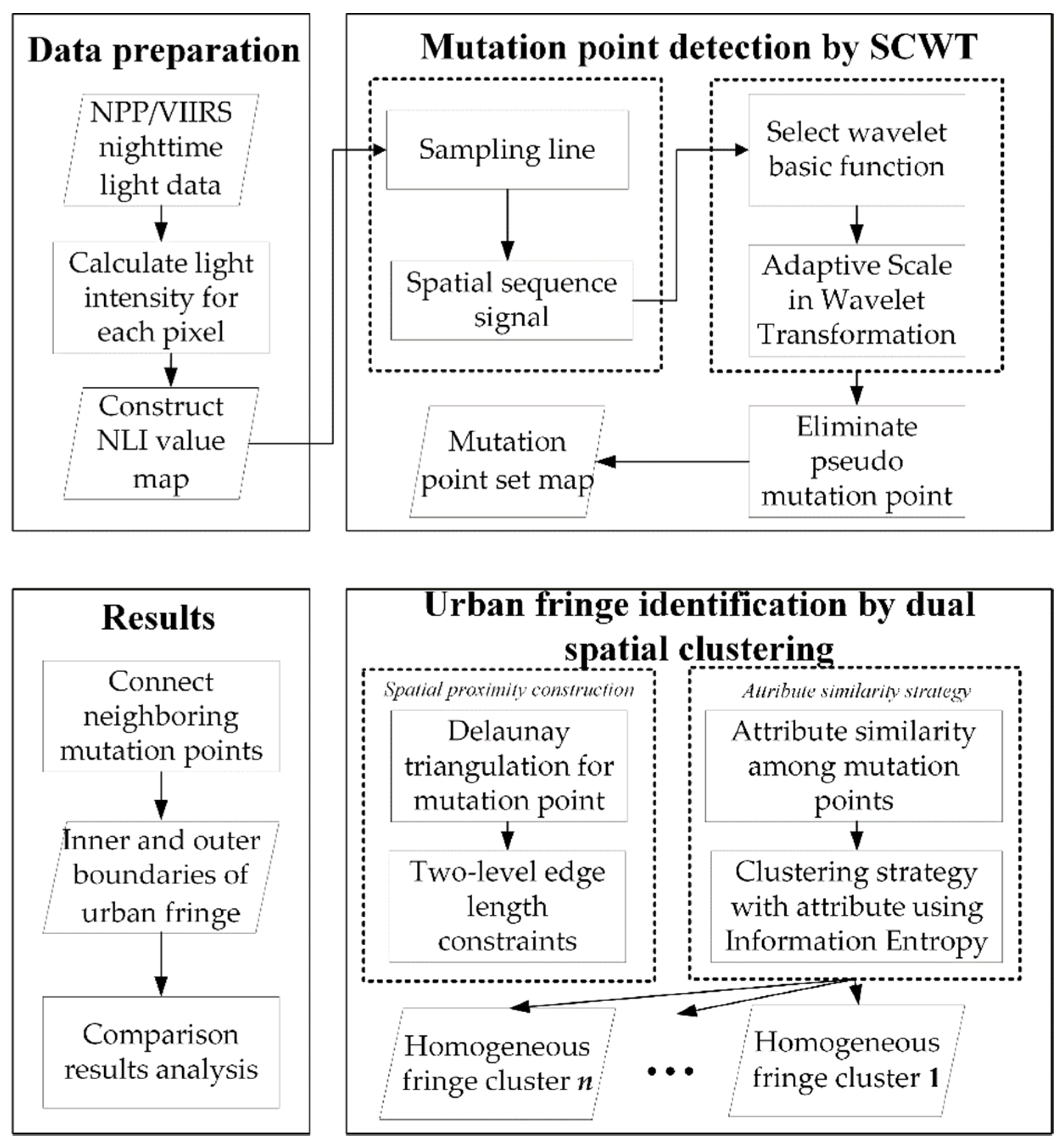
Figure 1. The sketch of the model to detect the urban fringe.
Remotesensing 14 06126 g001
Figure 2. Study region: (a) Location of the study region; (b) NPP/VIIRS nighttime light data in 2018; and (c) The NLI index’s spatial pattern at a grid scale of 1 km.
Remotesensing 14 06126 g002
Figure 3. Wavelet transform coefficients versus the scales.
Remotesensing 14 06126 g003
Figure 4. Elimination of “pseudo” mutation point: (a) “maximum module” of wavelet transform coefficients; (b) “pseudo” mutation points detected by k-standard deviations.
Remotesensing 14 06126 g004
Figure 5. Attribute clustering based on the modified method: (a) simulated data with attribute; (b) spatial clustering regarding attribute similarity; (c) curve graph of θ   score and the index of PBM.
Remotesensing 14 06126 g005
Figure 6. Detecting the mutation points by the sampling lines in 360 orientations.
Remotesensing 14 06126 g006
Figure 7. NLI index space sequence curve of the sampling line.
Remotesensing 14 06126 g007
Figure 8. Mutation points mapping result.
Remotesensing 14 06126 g008
Figure 9. Spatial proximity relationships between mutation points: (a) construction of DT; (b) global and local edge-length constraints.
Remotesensing 14 06126 g009
Figure 10. Detection of urban fringe in Nanjing: (a) clustering result; (b) spatial boundaries of urban fringes.
Remotesensing 14 06126 g010
Figure 11. Detection of urban fringe with different slicing thresholds: (a) result with k = 0.0; (b) result with k = 3.0.
Remotesensing 14 06126 g011
Figure 12. Detection of urban fringe with different dual spatial clustering methods: (a) Mk-means clustering (k = 10); (b) DBSC clustering.
Remotesensing 14 06126 g012
Figure 13. Detection of urban fringe with NASA’s Black Marble product: (a) Black Marble nighttime light data (VNP46A4) in 2018; (b) Detected mutation points at a grid scale of 0.5 km; (c) clustering results by our method; (d) Spatial boundaries of urban fringes.
Remotesensing 14 06126 g013aRemotesensing 14 06126 g013b
Table 1. Statistical information of the clustering results by our method.
C1C2C3C4C5C6C7C8C9C10C11
Number195152055151210201398
Mean value69.236.750.263.278.345.668.543.315.636.76.9
Standard deviation15.47.38.612.98.47.36.68.96.46.27.8
C13C14C16C17C18C22C23C25C28C29C32
Number8871268811765
Mean value43.526.536.553.169.252.170.140.218.139.310.9
Standard deviation7.66.56.37.27.66.57.16.86.95.24.8
Table 2. The clustering results from statistical information.
Our MethodDBSCMk-Means
Number of clusters224510
Number of noises15420
Urban fringe segment9127
SD of mean values of clusters20.5634.1511.39
Table 3. NLF of urban fringe areas with various approaches.
Our MethodDBSCMk-Means
NFL of urban fringe17.4615.138.65
RS index0.730.530.21
Publisher’s Note: MDPI stays neutral with regard to jurisdictional claims in published maps and institutional affiliations.