
Optimizing Landsat Next Shortwave Infrared Bands for Crop Residue Characterization

 , ,
, ,  , , , and
Abstract
1. Introduction
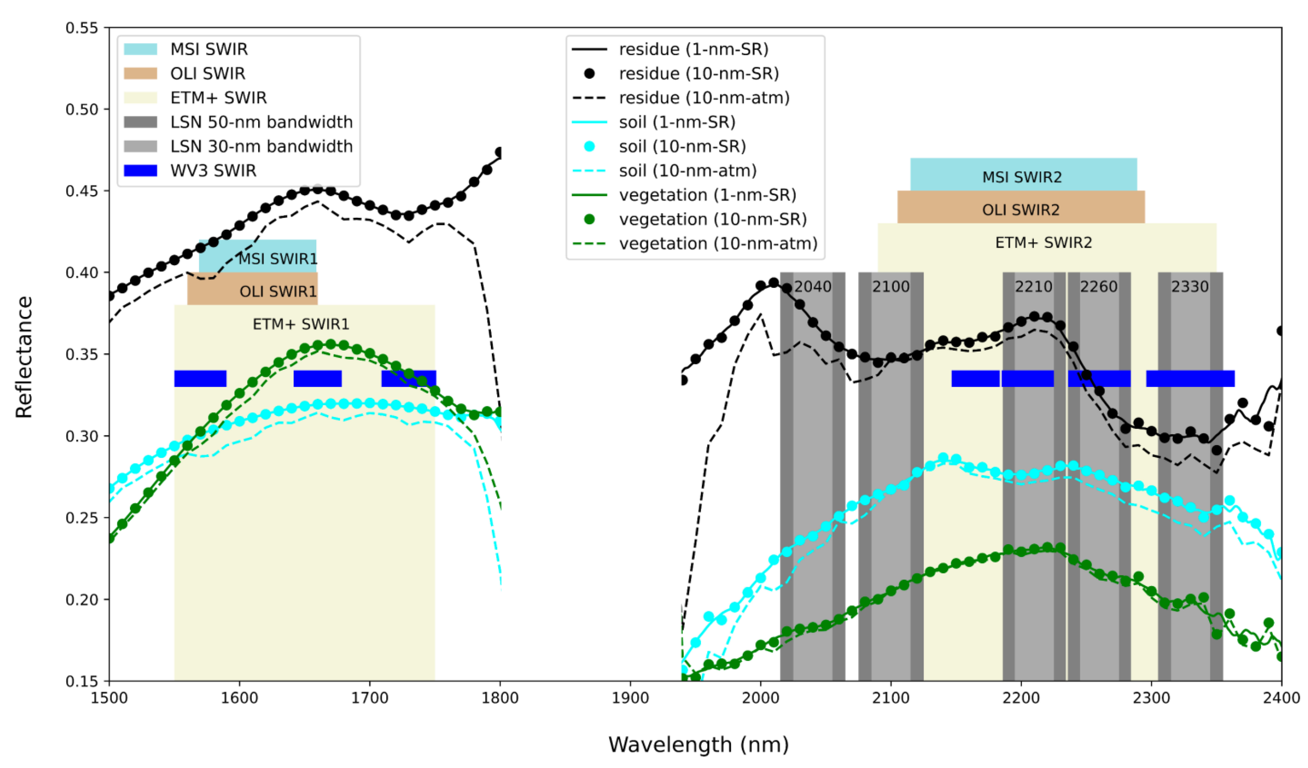
2. Materials and Methods
2.1. Two-Band Iterative Wavelength Shift Approach
2.2. Three-Band Iterative Wavelength Shift Approach
2.3. Iterative Wavelength Shift Approach Applied to BARC Spectra Datasets
2.4. Assessment of Moisture and Green Vegetation Impacts on Crop Residue Estimation
3. Results
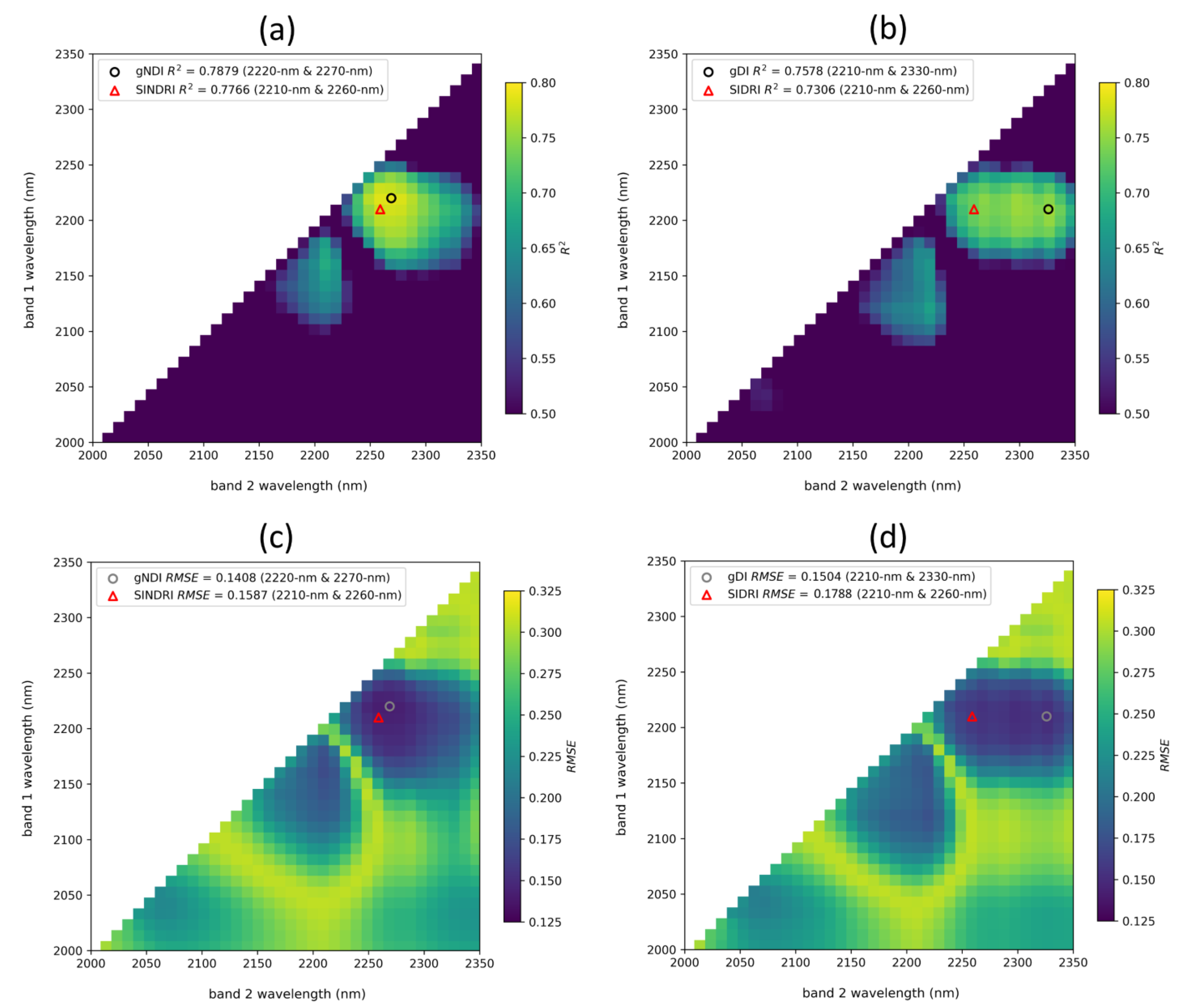
3.1. Two-Band Wavelength Shift Analysis Using the 10 nm BARC Dataset
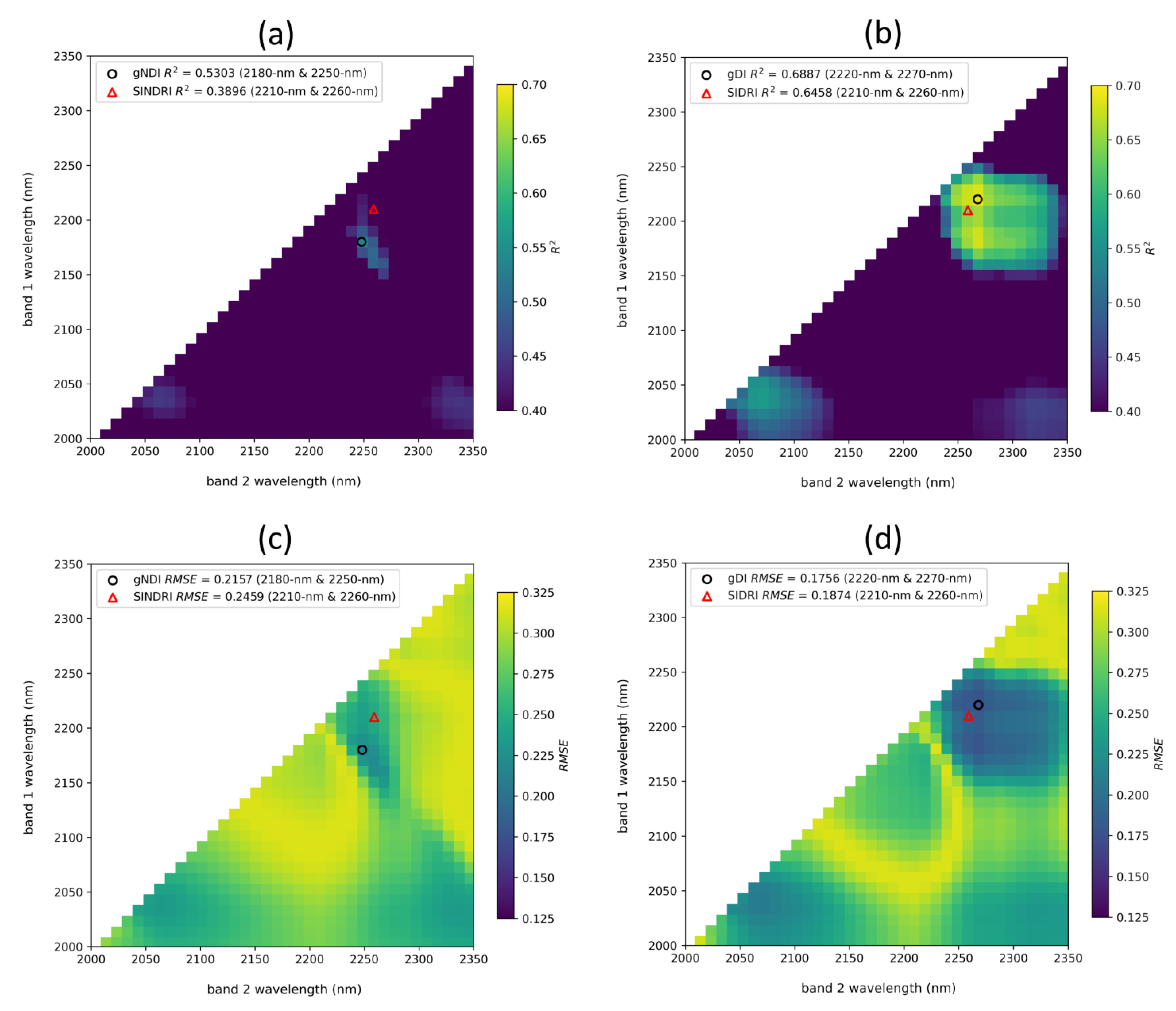
3.2. Two-Band Wavelength Shift Analysis Using the 1 nm Interval BARC Dataset
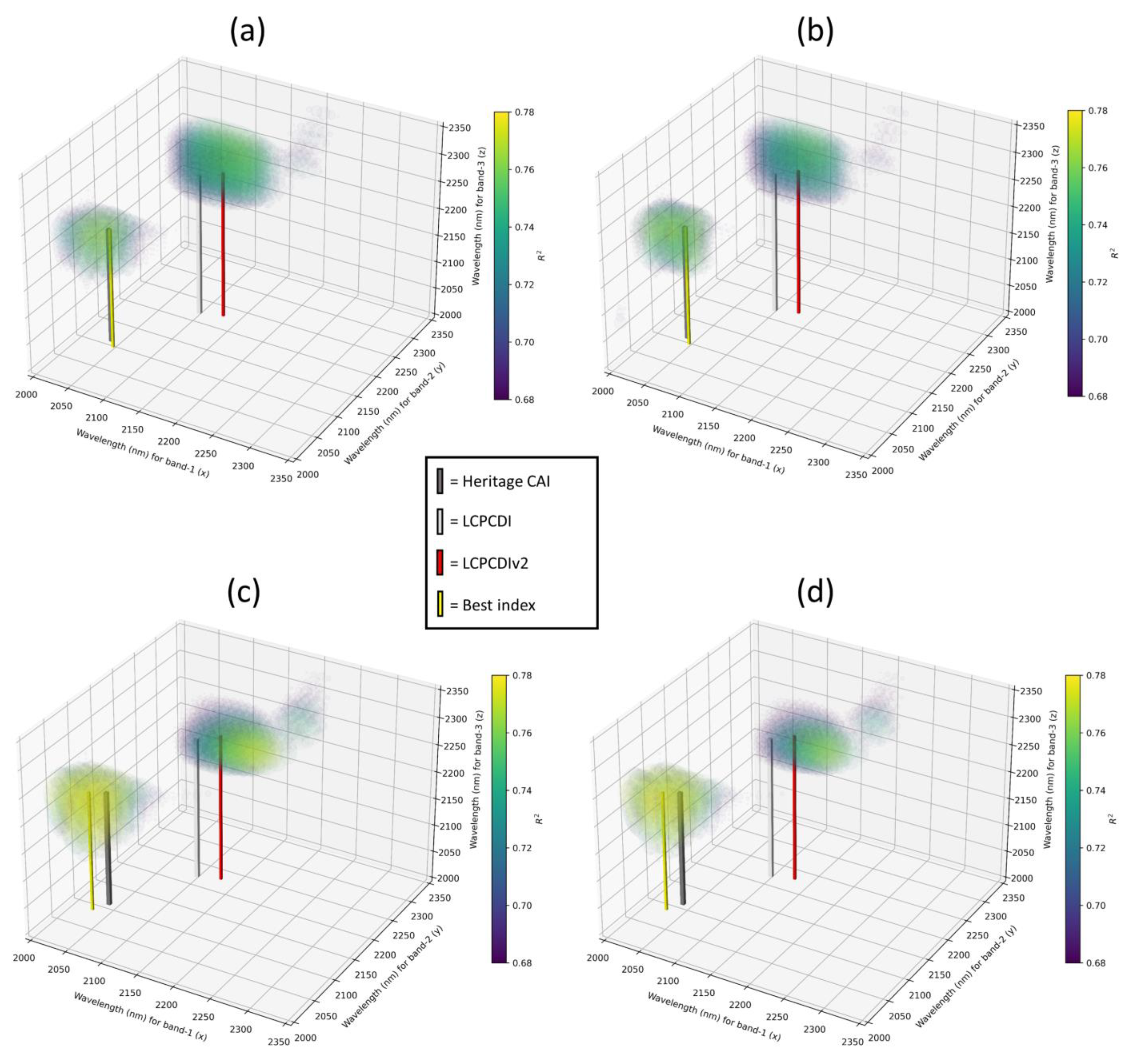
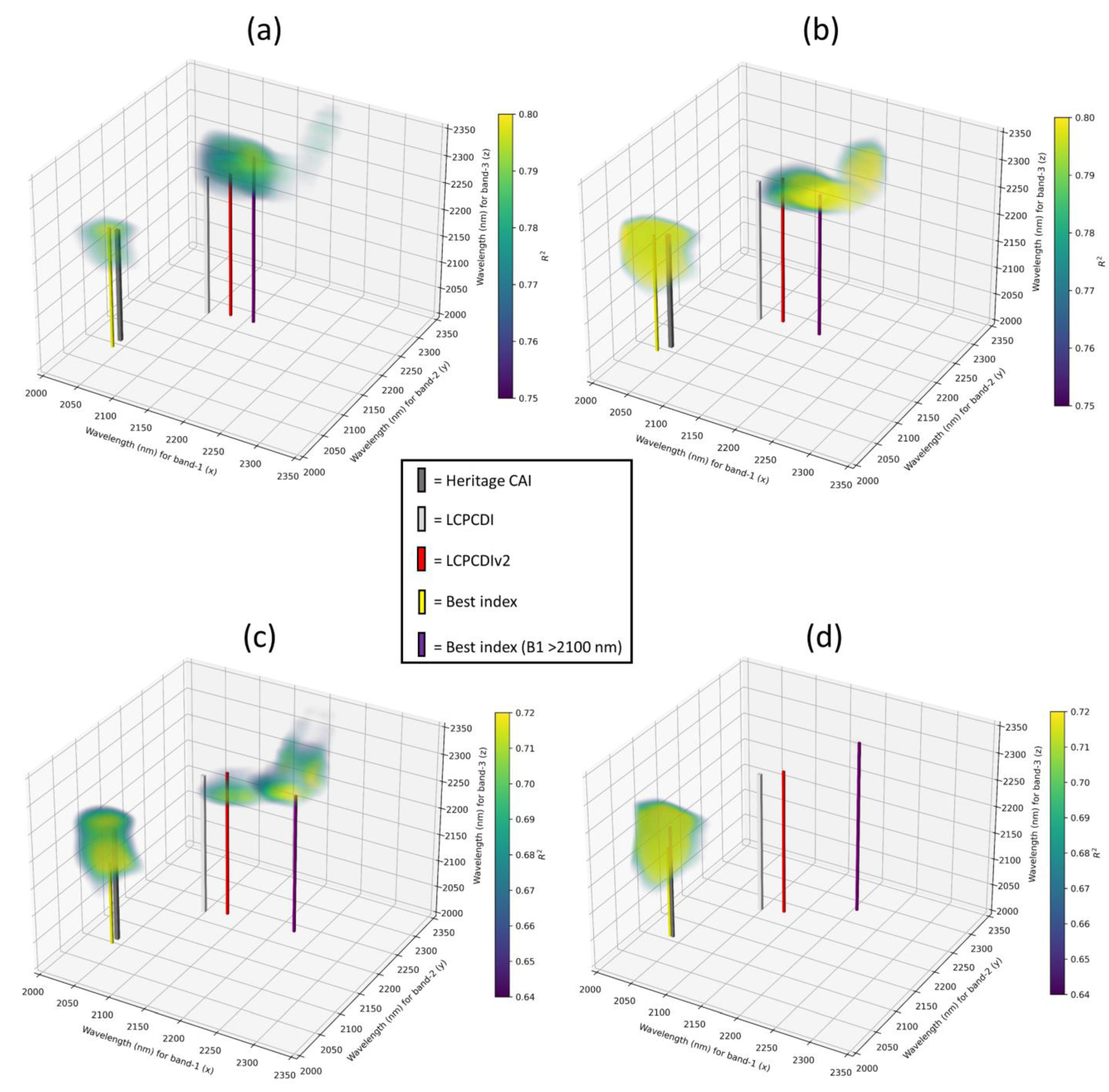
3.3. Three-Band Wavelength Shift Analysis Using the 10 nm BARC Dataset
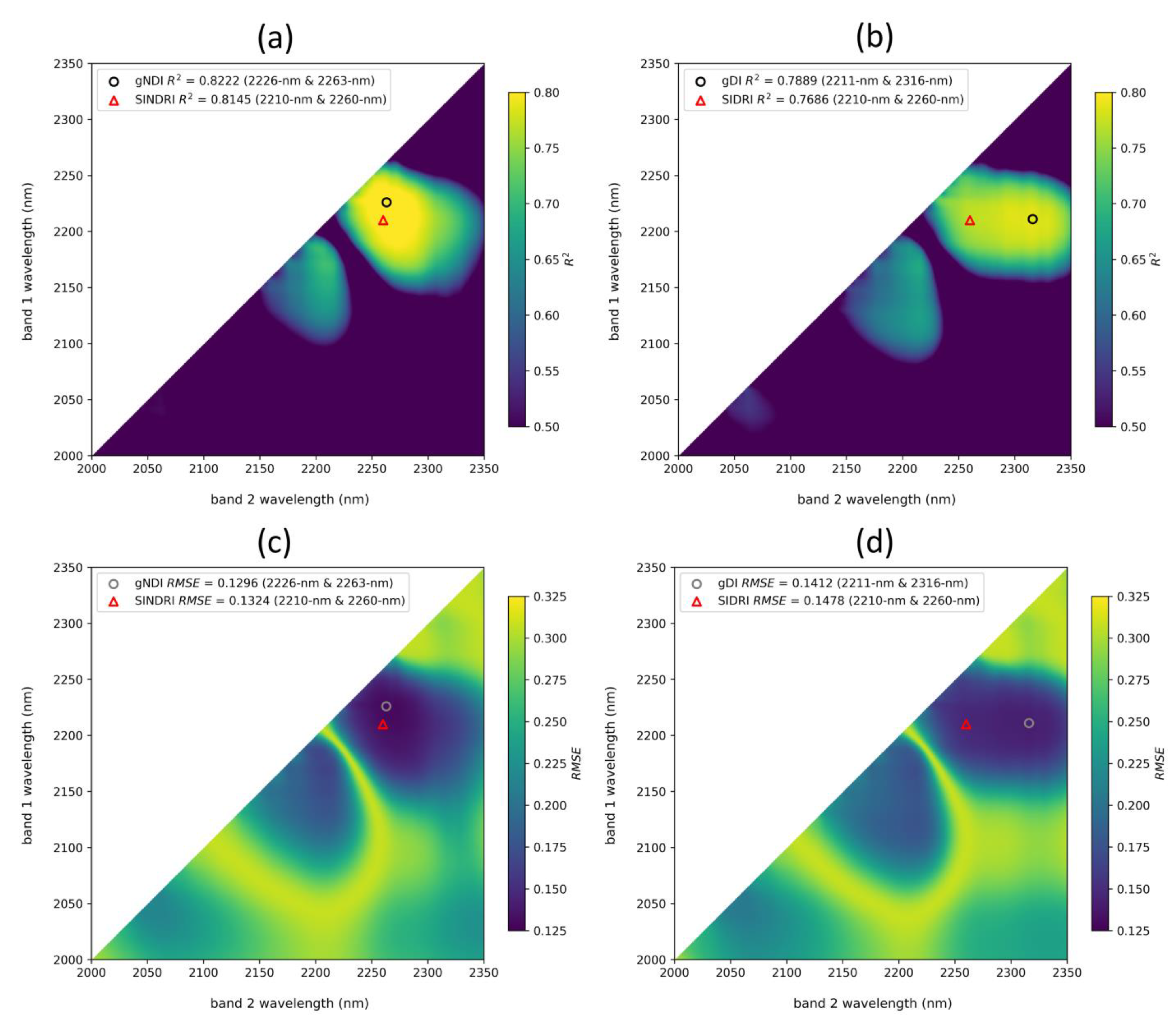
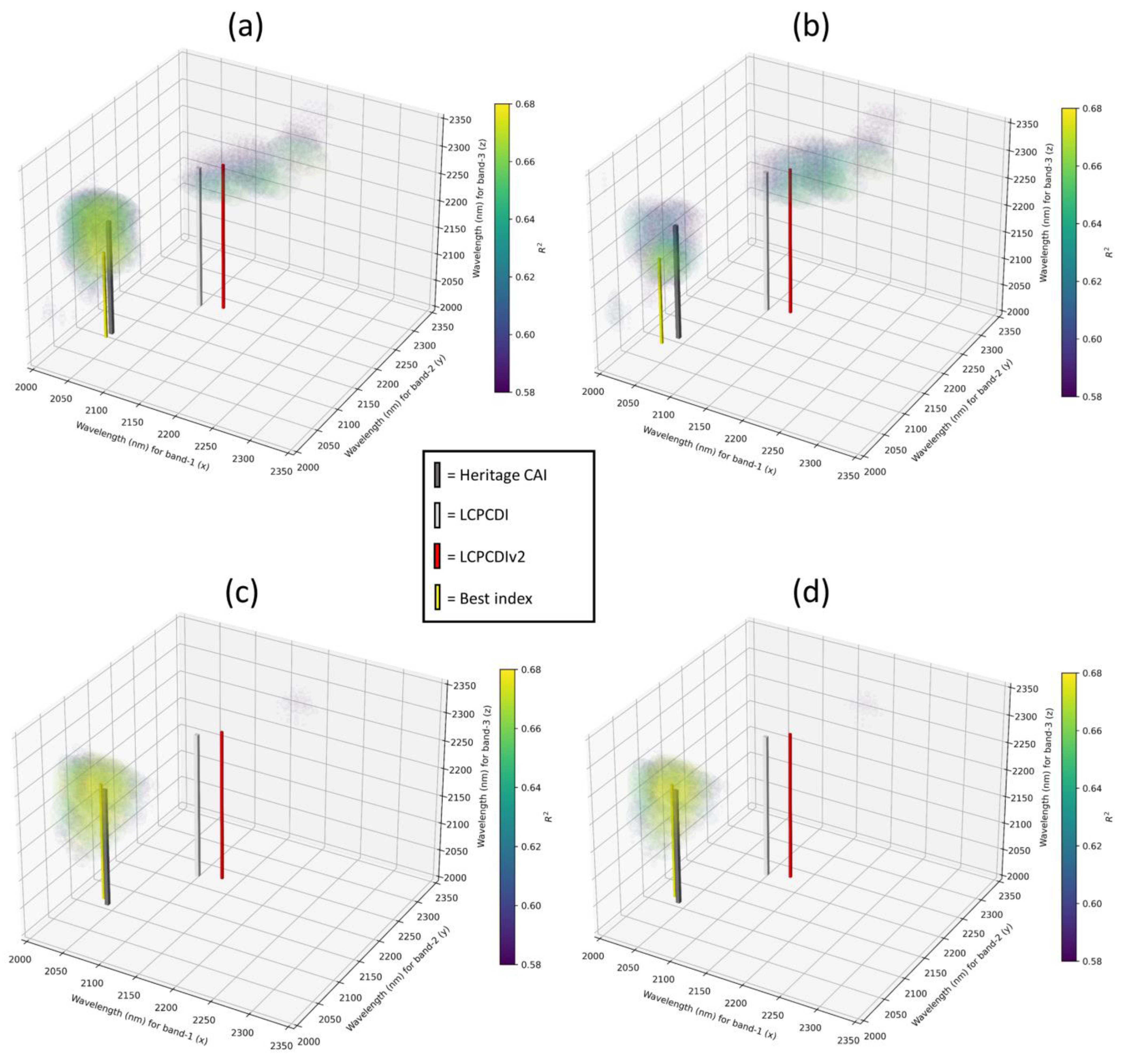
3.4. Three-Band Wavelength Shift Analysis Using the 1 nm Interval BARC Dataset
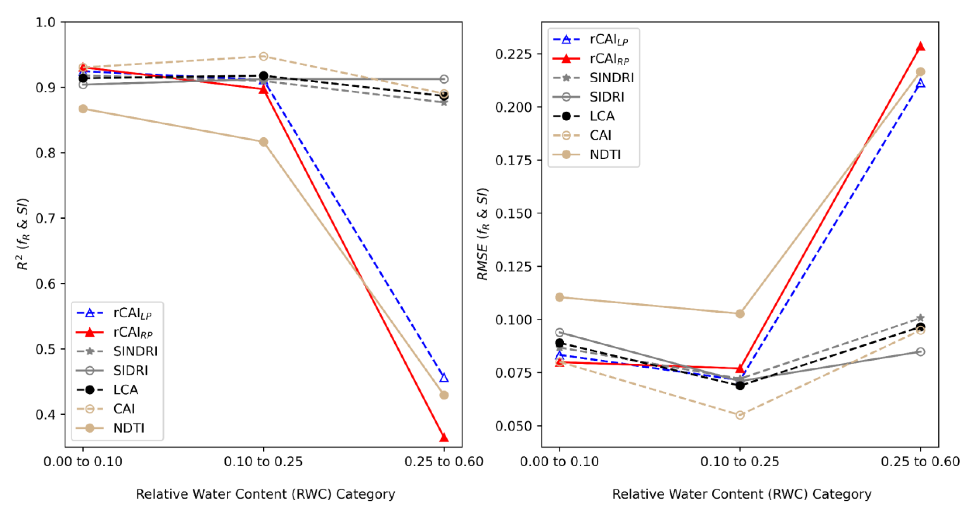
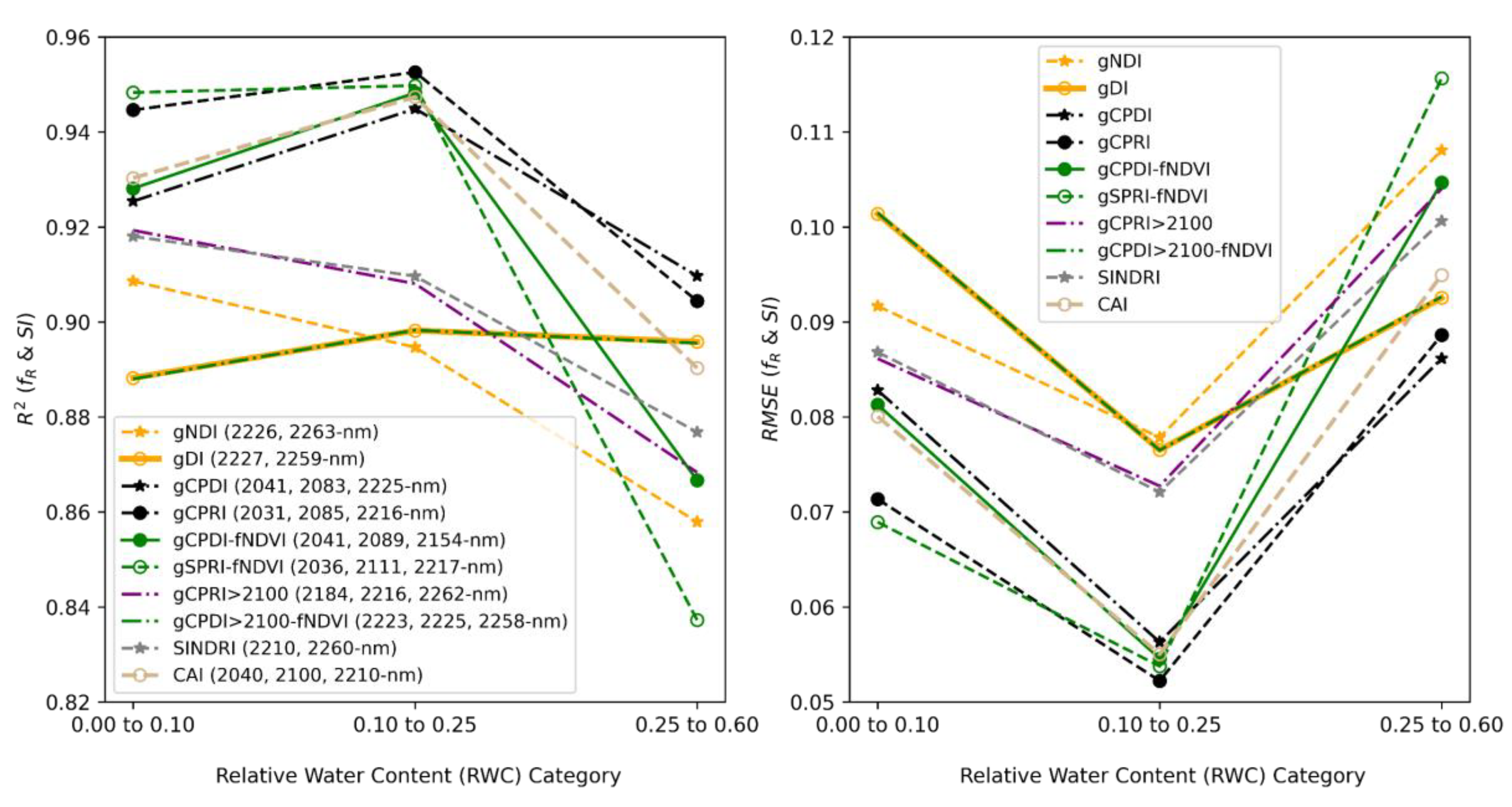
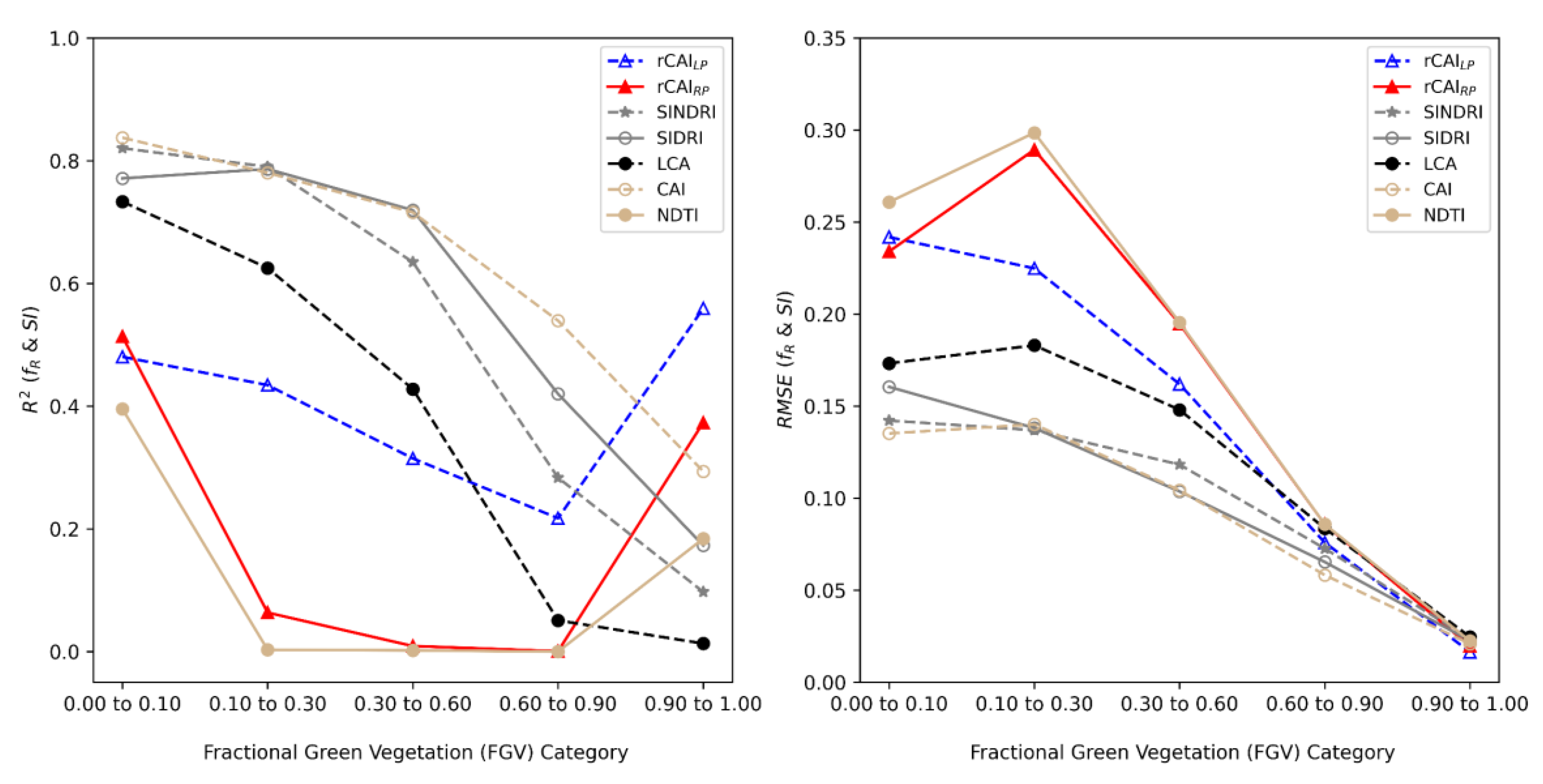
3.5. Moisture and Green Vegetation Impacts on Fractional Crop Residue (fR) Cover Estimation
4. Discussion
5. Conclusions
Supplementary Materials
Author Contributions
Funding
Data Availability Statement
Conflicts of Interest
Disclaimer
Abbreviations
| atm | abbreviation for spectra with atmospheric residuals |
| AVIRIS | Airborne Visible/Infrared Imaging Spectrometer |
| BARC | Beltsville Agricultural Research Center (USDA) |
| CAI | Cellulose Absorption Index |
| ETM+ | Enhanced Thematic Mapper Plus (on Landsat 7) |
| fGV | Fractional green vegetation cover |
| fR | Fractional crop residue cover |
| fS | Fractional soil cover |
| gCPDI | Generalized Center Peak Difference Index (three-band) |
| gCPRI | Generalized Center Peak Ratio Index (three-band) |
| gDI | Generalized Difference Index (two-band) |
| gNDI | Generalized Normalized Difference Index (two-band) |
| gSPRI | Generalized Side Peak Ratio Index (three-band) |
| LCA | Lignin Cellulose Absorption index |
| LCPCDI | Lignin Cellulose Peak Center Difference Index |
| LCPCDIv2 | Lignin Cellulose Peak Center Difference Index version 2 |
| MSI | Multispectral Instrument (on Sentinel-2) |
| NDTI | Normalized Difference Tillage Index |
| NDVI | Normalized Difference Vegetation Index |
| NPV | Non-photosynthetic vegetation |
| OLI | Operational Land Imager (on Landsats 8 and 9) |
| PRISMA | PRecursore IperSpettrale della Missione Applicativa |
| rCAILP | Ratio CAI—Left Peak (two-band) |
| rCAIRP | Ratio CAI—Right Peak (two-band) |
| RWC | Relative water content |
| SI | Spectral index |
| SIDRI | Shortwave Infrared Difference Residue Index |
| SINDRI | Shortwave Infrared Normalized Difference Residue Index |
| SR | Surface reflectance |
| SWIR | Shortwave infrared |
| SWIR1 | Shorter wavelength SWIR region and band for OLI and MSI (~1600 nm) |
| SWIR2 | Longer wavelength SWIR region and band for OLI and MSI (~2200 nm) |
| TM | Thematic Mapper (on Landsat 5) |
| WV3 | WorldView-3 |
References
- Wu, Z.; Snyder, G.; Vadnais, C.; Arora, R.; Babcock, M.; Stensaas, G.; Doucette, P.; Newman, T. User needs for future Landsat missions. Remote Sens. Environ. 2019, 231, 111214. [Google Scholar] [CrossRef]
- NASA, Goddard Space Flight Center. Landsat Next Request for Information (RFI). 2020. Available online: https://sam.gov/opp/09a18f980f67449fa10608ecb0924883/view?keywords=%22Landsat%20Next%22 (accessed on 30 October 2020).
- Lal, R. The Role of Residues Management in Sustainable Agricultural Systems. J. Sustain. Agric. 1995, 5, 51–78. [Google Scholar] [CrossRef]
- Magdoff, F.; Weil, R. Soil Organic Matter Management Strategies. In Soil Organic Matter in Sustainable Agriculture; CRC Press: Boca Raton, FL, USA, 2004. [Google Scholar] [CrossRef]
- Delgado, J.A. Crop residue is a key for sustaining maximum food production and for conservation of our biosphere. J. Soil Water Conserv. 2010, 65, 111A–116A. [Google Scholar] [CrossRef]
- Palm, C.; Blanco-Canqui, H.; DeClerck, F.; Gatere, L.; Grace, P. Conservation agriculture and ecosystem services: An overview. Agric. Ecosyst. Environ. 2014, 187, 87–105. [Google Scholar] [CrossRef]
- Zheng, B.; Campbell, J.B.; Serbin, G.; Daughtry, C.S.T. Multitemporal remote sensing of crop residue cover and tillage practices: A validation of the minNDTI strategy in the United States. J. Soil Water Conserv. 2013, 68, 120–131. [Google Scholar] [CrossRef]
- Conservation Technology Information Center. Procedures for Using the Cropland Roadside Transect Survey for Obtaining Tillage Crop Residue Data; Conservation Technology Information Center, Purdue University: West Lafayette, IN, USA, 2009; Available online: http://www.ctic.org (accessed on 5 May 2022).
- Masek, J.G.; Wulder, M.A.; Markham, B.; McCorkel, J.; Crawford, C.J.; Storey, J.; Jenstrom, D.T. Landsat 9: Empowering open science and applications through continuity. Remote Sens. Environ. 2020, 248, 111968. [Google Scholar] [CrossRef]
- U.S. Geological Survey. What are the Band Designations for the Landsat Satellites? 2022. Available online: https://www.usgs.gov/faqs/what-are-band-designations-landsat-satellites (accessed on 21 May 2022).
- Daughtry, C.S.T.; Doraiswamy, P.C.; Hunt, E.R.; Stern, A.J.; McMurtrey, J.E.; Prueger, J.H. Remote sensing of crop residue cover and soil tillage intensity. Soil Tillage Res. 2006, 91, 101–108. [Google Scholar] [CrossRef]
- Knight, E.J.; Kvaran, G. Landsat-8 Operational Land Imager Design, Characterization and Performance. Remote Sens. 2014, 6, 10286–10305. [Google Scholar] [CrossRef]
- ACCP. Accelerated Canopy Chemistry Program Final Report to NASA-EOS-IWG; National Aeronautics and Space Administration: Washington, DC, USA, 1994. Available online: http://daac.ornl.gov/ACCP/accp.html (accessed on 23 May 2022).
- Serrano, L.; Penuelas, J.; Ustin, S.L. Remote sensing of nitrogen and lignin in Mediterranean vegetation from AVIRIS data: Decomposing biochemical from structural signals. Remote Sens. Environ. 2002, 81, 355–364. [Google Scholar] [CrossRef]
- Kokaly, R.F.; Despain, D.G.; Clark, R.N.; Livo, K.E. Mapping vegetation in Yellowstone National Park using spectral feature analysis of AVIRIS data. Remote Sens. Environ. 2003, 84, 437–456. [Google Scholar] [CrossRef]
- Kokaly, R.F.; Rockwell, B.W.; Haire, S.L.; King, T.V. Characterization of post-fire surface cover, soils, and burn severity at the Cerro Grande Fire, New Mexico, using hyperspectral and multispectral remote sensing. Remote Sens. Environ. 2007, 106, 305–325. [Google Scholar] [CrossRef]
- Pepe, M.; Pompilio, L.; Gioli, B.; Busetto, L.; Boschetti, M. Detection and Classification of Non-Photosynthetic Vegetation from PRISMA Hyperspectral Data in Croplands. Remote Sens. 2020, 12, 3903. [Google Scholar] [CrossRef]
- Van Deventer, A.P.; Ward, A.D.; Gowda, P.M.; Lyon, J.G. Using thematic mapper data to identify contrasting soil plains and tillage practices. Photogramm. Eng. Remote Sens. 1997, 63, 87–93. [Google Scholar]
- Jin, X.; Ma, J.; Wen, Z.; Song, K. Estimation of maize residue cover using Landsat-8 OLI image spectral information and textural features. Remote Sens. 2015, 7, 14559–14575. [Google Scholar] [CrossRef]
- Hively, W.D.; Lamb, B.T.; Daughtry, C.S.T.; Shermeyer, J.; McCarty, G.W.; Quemada, M. Mapping crop residue and tillage intensity using WorldView-3 satellite shortwave infrared residue indices. Remote Sens. 2018, 10, 1657. [Google Scholar] [CrossRef]
- Najafi, P.; Navid, H.; Feizizadeh, B.; Eskandari, I.; Blaschke, T. Fuzzy object-based image analysis methods using Sentinel-2A and Landsat-8 data to map and characterize soil surface residue. Remote Sens. 2019, 11, 2583. [Google Scholar] [CrossRef]
- Azzari, G.; Grassini, P.; Edreira, J.I.R.; Conley, S.; Mourtzinis, S.; Lobell, D.B. Satellite mapping of tillage practices in the North Central US region from 2005 to 2016. Remote Sens. Environ. 2019, 221, 417–429. [Google Scholar] [CrossRef]
- Beeson, P.C.; Daughtry, C.S.T.; Wallander, S.A. Estimates of conservation tillage practices using Landsat archive. Remote Sens. 2020, 12, 2665. [Google Scholar] [CrossRef]
- Hagen, S.C.; Delgado, G.; Ingraham, P.; Cooke, I.; Emery, R.; Fisk, J.P.; Melendy, L.; Olson, T.; Patti, S.; Rubin, N.; et al. Mapping conservation management practices and outcomes in the corn belt using the operational tillage information system (Optis) and the denitrification–decomposition (DNDC) model. Land 2020, 9, 408. [Google Scholar] [CrossRef]
- Yue, J.; Tian, Q.; Dong, X.; Xu, N. Using broadband crop residue angle index to estimate the fractional cover of vegetation, crop residue, and bare soil in cropland systems. Remote Sens. Environ. 2020, 237, 111538. [Google Scholar] [CrossRef]
- Yue, J.; Fu, Y.; Guo, W.; Feng, H.; Qiao, H. Estimating fractional coverage of crop, crop residue, and bare soil using shortwave infrared angle index and Sentinel-2 MSI. Int. J. Remote Sens. 2022, 43, 1253–1273. [Google Scholar] [CrossRef]
- South, S.; Qi, J.; Lusch, D.P. Optimal classification methods for mapping agricultural tillage practices. Remote Sens. Environ. 2004, 91, 90–97. [Google Scholar] [CrossRef]
- Bannari, A.; Pacheco, A.; Staenz, K.; McNairn, H.; Omari, K. Estimating and mapping crop residues cover on agricultural lands using hyperspectral and IKONOS data. Remote Sens. Environ. 2006, 104, 447–459. [Google Scholar] [CrossRef]
- Yue, J.; Tian, Q.; Dong, X.; Xu, K.; Zhou, C. Using hyperspectral crop residue angle index to estimate maize and winter-wheat residue cover: A laboratory study. Remote Sens. 2019, 11, 807. [Google Scholar] [CrossRef]
- Daughtry, C.S.T.; Hunt, E.R. Mitigating the effects of soil and residue water contents on remotely sensed estimates of crop residue cover. Remote Sens. Environ. 2008, 112, 1647–1657. [Google Scholar] [CrossRef]
- Serbin, G.; Daughtry, C.S.T.; Hunt, E.R.; Brown, D.J.; McCarty, G.W. Effect of Soil Spectral Properties on Remote Sensing of Crop Residue Cover. Soil Sci. Soc. Am. J. 2009, 73, 1545–1558. [Google Scholar] [CrossRef]
- Quemada, M.; Hively, W.D.; Daughtry, C.S.T.; Lamb, B.T.; Shermeyer, J. Improved crop residue cover estimates obtained by coupling spectral indices for residue and moisture. Remote Sens. Environ. 2018, 206, 33–44. [Google Scholar] [CrossRef]
- Anderegg, W.R.L.; Anderegg, L.D.L.; Huang, C.Y. Testing early warning metrics for drought-induced tree physiological stress and mortality. Glob. Chang. Biol. 2019, 25, 2459–2469. [Google Scholar] [CrossRef]
- Coates, A.R.; Dennison, P.E.; Roberts, D.A.; Roth, K.L. Monitoring the impacts of severe drought on Southern California chaparral species using hyperspectral and thermal infrared imagery. Remote Sens. 2015, 7, 14200–14215. [Google Scholar] [CrossRef]
- Bai, X.; Zhao, W.; Ji, S.; Qiao, R.; Dong, C.; Chang, X. Estimating fractional cover of non-photosynthetic vegetation for various grasslands based on CAI and DFI. Ecol. Indic. 2021, 131, 108252. [Google Scholar] [CrossRef]
- Lugassi, R.; Chudnovsky, A.; Zaady, E.; Dvash, L.; Goldshleger, N. Spectral Slope as an Indicator of Pasture Quality. Remote Sens. 2015, 7, 256–274. [Google Scholar] [CrossRef]
- Hively, W.D.; Lamb, B.T.; Daughtry, C.S.T.; Serbin, G.; Dennison, P.; Kokaly, R.F.; Wu, Z.; Masek, J.G. Evaluation of SWIR crop residue bands for the Landsat Next mission. Remote Sens. 2021, 13, 3718. [Google Scholar] [CrossRef]
- Kokaly, R.F.; Asner, G.P.; Ollinger, S.V.; Martin, M.E.; Wessman, C.A. Characterizing canopy biochemistry from imaging spectroscopy and its application to ecosystem studies. Remote Sens. Environ. 2009, 113, S78–S91. [Google Scholar] [CrossRef]
- Dennison, P.E.; Qi, Y.; Meerdink, S.K.; Kokaly, R.F.; Thompson, D.R.; Daughtry, C.S.T.; Quemada, M.; Roberts, D.A.; Gader, P.D.; Wetherley, E.B.; et al. Comparison of methods for modeling fractional cover using simulated satellite hyperspectral imager spectra. Remote Sens. 2019, 11, 2072. [Google Scholar] [CrossRef]
- Quemada, M.; Daughtry, C.S.T. Spectral indices to improve crop residue cover estimation under varying moisture conditions. Remote Sens. 2016, 8, 660. [Google Scholar] [CrossRef]
- Serbin, G.; Hunt, E.R.; Daughtry, C.S.T.; McCarty, G.W.; Doraiswamy, P.C. An improved ASTER index for remote sensing of crop residue. Remote Sens. 2009, 1, 971–991. [Google Scholar] [CrossRef]
- Elvidge, C.D. Visible and near infrared reflectance characteristics of dry plant materials. Int. J. Remote Sens. 1990, 11, 1775–1795. [Google Scholar] [CrossRef]
- Nagler, P.L.; Daughtry, C.S.T.; Goward, S.N. Plant litter and soil reflectance. Remote Sens. Environ. 2000, 71, 207–215. [Google Scholar] [CrossRef]
- Daughtry, C.S.T.; Hunt, E.R.; Doraiswamy, P.C.; McMurtrey, J.E. Remote sensing the spatial distribution of crop residues. Agron. J. 2005, 97, 864–871. [Google Scholar] [CrossRef]
- Prabhakara, K.; Hively, W.D.; McCarty, G.W. Evaluating the relationship between biomass, percent groundcover and remote sensing indices across six winter cover crop fields in Maryland, United States. Int. J. Appl. Earth Obs. Geoinf. 2015, 39, 88–102. [Google Scholar] [CrossRef]
- Philpot, W.; Jacquemoud, S.; Tian, J. ND-space: Normalized difference spectral mapping. Remote Sens. Environ. 2021, 264, 112622. [Google Scholar] [CrossRef]
- Wang, L.; Hunt, E.R., Jr.; Qu, J.J.; Hao, X.; Daughtry, C.S.T. Remote sensing of fuel moisture content from ratios of narrow-band vegetation water and dry-matter indices. Remote Sens. Environ. 2013, 129, 103–110. [Google Scholar] [CrossRef]
- Thoma, D.P.; Gupta, S.C.; Bauer, M.E. Evaluation of optical remote sensing models for crop residue cover assessment. J. Soil Water Conserv. 2004, 59, 224–233. [Google Scholar]
- Hively, W.D.; Lamb, B.T.; Daughtry, C.S.T.; Serbin, G.; Dennison, P. Reflectance Spectra of Agricultural Field Conditions Supporting Remote Sensing Evaluation of Non-Photosynthetic Vegetative Cover (version 1.1); U.S. Geological Survey: Reston, VI, USA, 2021. [CrossRef]


| Index | NDVI | n | R2 | RMSE | Band-1 | Band-2 |
|---|---|---|---|---|---|---|
| gNDI-SR | <0.3 | 650 | 0.7879 | 0.1408 | 2220 | 2270 |
| gNDI-atm | <0.3 | 650 | 0.7734 | 0.1458 | 2220 | 2270 |
| gDI-SR | <0.3 | 650 | 0.7578 | 0.1504 | 2210 | 2330 |
| gDI-atm | <0.3 | 650 | 0.7428 | 0.1553 | 2210 | 2330 |
| SINDRI-SR | <0.3 | 650 | 0.7766 | 0.1587 | 2210 | 2260 |
| SINDRI-atm | <0.3 | 650 | 0.7610 | 0.1653 | 2210 | 2260 |
| SIDRI-SR | <0.3 | 650 | 0.7306 | 0.1788 | 2210 | 2260 |
| SIDRI-atm | <0.3 | 650 | 0.7089 | 0.1783 | 2210 | 2260 |
| gNDI-SR | full | 916 | 0.5303 | 0.2157 | 2180 | 2250 |
| gNDI-atm | full | 916 | 0.4709 | 0.2290 | 2180 | 2250 |
| gDI-SR | full | 916 | 0.6887 | 0.1756 | 2220 | 2270 |
| gDI-atm | full | 916 | 0.6870 | 0.1761 | 2220 | 2270 |
| SINDRI-SR | full | 916 | 0.3896 | 0.2459 | 2210 | 2260 |
| SINDRI-atm | full | 916 | 0.3613 | 0.2516 | 2210 | 2260 |
| SIDRI-SR | full | 916 | 0.6458 | 0.1874 | 2210 | 2260 |
| SIDRI-atm | full | 916 | 0.6505 | 0.1861 | 2210 | 2260 |
| Index | NDVI | n | R2 | RMSE | Band-1 | Band-2 |
|---|---|---|---|---|---|---|
| gNDI | <0.3 | 643 | 0.8222 | 0.1296 | 2226 | 2263 |
| gDI | <0.3 | 643 | 0.7889 | 0.1412 | 2211 | 2316 |
| SINDRI | <0.3 | 643 | 0.8145 | 0.1324 | 2210 | 2260 |
| SIDRI | <0.3 | 643 | 0.7686 | 0.1478 | 2210 | 2260 |
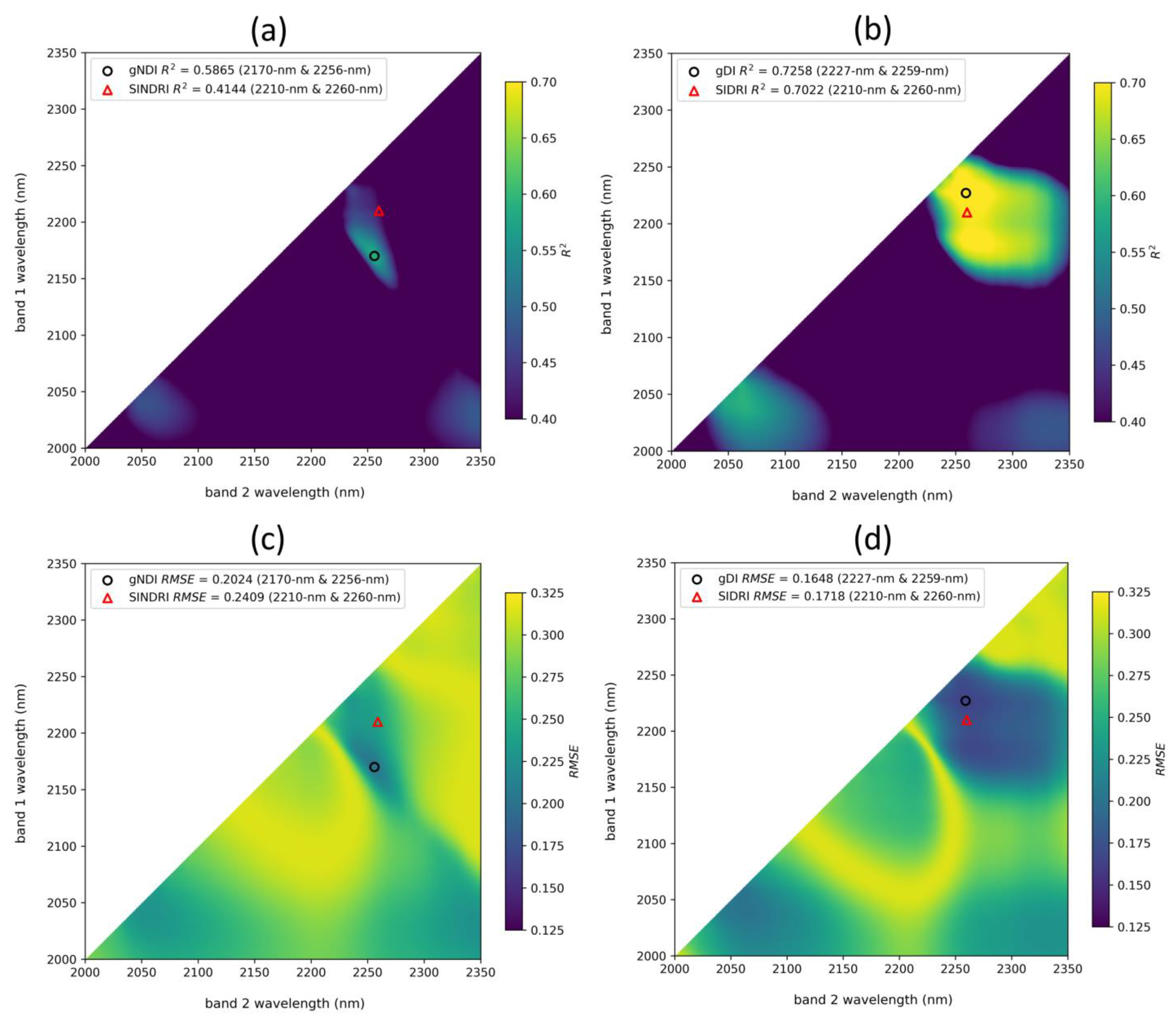
| gNDI | full | 916 | 0.5865 | 0.2024 | 2170 | 2256 |
| gDI | full | 916 | 0.7258 | 0.1648 | 2227 | 2259 |
| SINDRI | full | 916 | 0.4144 | 0.2409 | 2210 | 2260 |
| SIDRI | full | 916 | 0.7022 | 0.1718 | 2210 | 2260 |
| Index | NDVI | n | R2 | RMSE | Band-1 | Band-2 | Band-3 |
|---|---|---|---|---|---|---|---|
| gCPDI-SR | <0.3 | 650 | 0.7822 | 0.1427 | 2050 | 2090 | 2220 |
| gCPDI-atm | <0.3 | 650 | 0.7816 | 0.1431 | 2050 | 2090 | 2220 |
| gSPDI-SR | <0.3 | 650 | 0.7822 | 0.1427 | 2050 | 2090 | 2220 |
| gSPDI-atm | <0.3 | 650 | 0.7816 | 0.1431 | 2050 | 2090 | 2220 |
| gCPRI-SR | <0.3 | 650 | 0.8148 | 0.1315 | 2030 | 2080 | 2220 |
| gCPRI-atm | <0.3 | 650 | 0.8082 | 0.1341 | 2030 | 2080 | 2220 |
| gSPRI-SR | <0.3 | 650 | 0.8121 | 0.1325 | 2030 | 2080 | 2220 |
| gSPRI-atm | <0.3 | 650 | 0.8026 | 0.1361 | 2030 | 2080 | 2220 |
| CAI-SR | <0.3 | 650 | 0.7486 | 0.1533 | 2040 | 2100 | 2210 |
| CAI-atm | <0.3 | 650 | 0.7507 | 0.1529 | 2040 | 2100 | 2210 |
| LCPCDI-SR | <0.3 | 650 | 0.7129 | 0.1638 | 2100 | 2210 | 2260 |
| LCPCDI-atm | <0.3 | 650 | 0.6947 | 0.1692 | 2100 | 2210 | 2260 |
| LCPCDIv2-SR | <0.3 | 650 | 0.7625 | 0.1490 | 2130 | 2220 | 2270 |
| LCPCDIv2-atm | <0.3 | 650 | 0.7516 | 0.1527 | 2130 | 2220 | 2270 |
| gCPDI-SR | full | 916 | 0.6941 | 0.1741 | 2040 | 2090 | 2160 |
| gCPDI-atm | full | 916 | 0.6830 | 0.1772 | 2030 | 2080 | 2160 |
| gSPDI-SR | full | 916 | 0.6941 | 0.1741 | 2040 | 2090 | 2160 |
| gSPDI-atm | full | 916 | 0.6830 | 0.1772 | 2030 | 2080 | 2160 |
| gCPRI-SR | full | 916 | 0.7148 | 0.1681 | 2030 | 2110 | 2210 |
| gCPRI-atm | full | 916 | 0.7143 | 0.1682 | 2030 | 2110 | 2210 |
| gSPRI-SR | full | 916 | 0.7176 | 0.1673 | 2030 | 2110 | 2210 |
| gSPRI-atm | full | 916 | 0.7171 | 0.1674 | 2030 | 2110 | 2210 |
| CAI-SR | full | 916 | 0.6716 | 0.1804 | 2040 | 2100 | 2210 |
| CAI-atm | full | 916 | 0.5807 | 0.2038 | 2040 | 2100 | 2210 |
| LCPCDI-SR | full | 916 | 0.4622 | 0.2308 | 2100 | 2210 | 2260 |
| LCPCDI-atm | full | 916 | 0.4381 | 0.2360 | 2100 | 2210 | 2260 |
| LCPCDIv2-SR | full | 916 | 0.5782 | 0.2044 | 2130 | 2220 | 2270 |
| LCPCDIv2-atm | full | 916 | 0.5564 | 0.2097 | 2130 | 2220 | 2270 |
| Index | NDVI | n | R2 | RMSE | Band-1 | Band-2 | Band-3 |
|---|---|---|---|---|---|---|---|
| gCPDI | <0.3 | 643 | 0.8021 | 0.1367 | 2041 | 2083 | 2225 |
| gSPDI | <0.3 | 643 | 0.8021 | 0.1367 | 2041 | 2083 | 2225 |
| gCPRI | <0.3 | 643 | 0.8397 | 0.1231 | 2031* | 2085 | 2216 |
| gSPRI | <0.3 | 643 | 0.8360 | 0.1244 | 2031 | 2084 | 2216 |
| gCPDI>2100 | <0.3 | 643 | 0.8009 | 0.1371 | 2163 | 2220 | 2313 |
| gSPDI>2100 | <0.3 | 643 | 0.8009 | 0.1371 | 2163 | 2220 | 2313 |
| gCPRI>2100 | <0.3 | 643 | 0.8262 | 0.1281 | 2184 | 2216 | 2262 |
| gSPRI>2100 | <0.3 | 643 | 0.8241 | 0.1289 | 2185 | 2216 | 2262 |
| CAI | <0.3 | 643 | 0.7714 | 0.1469 | 2040 | 2100 | 2210 |
| LCPCDI | <0.3 | 643 | 0.7466 | 0.1547 | 2100 | 2210 | 2260 |
| LCPCDIv2 | <0.3 | 643 | 0.7806 | 0.1440 | 2130 | 2220 | 2270 |
| gCPDI | full | 916 | 0.7338 | 0.1624 | 2041 | 2089 | 2154 |
| gSPDI | full | 916 | 0.7338 | 0.1624 | 2041 | 2089 | 2154 |
| gCPRI | full | 916 | 0.7567 | 0.1553 | 2036 | 2100 | 2169 |
| gSPRI | full | 916 | 0.7581 | 0.1548 | 2036 | 2111 | 2217 |
| gCPDI>2100 | full | 916 | 0.7260 | 0.1648 | 2223 | 2225 | 2258 |
| gSPDI>2100 | full | 916 | 0.7260 | 0.1648 | 2223 | 2225 | 2258 |
| gCPRI>2100 | full | 916 | 0.6517 | 0.1858 | 2208 | 2270 | 2320 |
| gSPRI>2100 | full | 916 | 0.6574 | 0.1843 | 2208 | 2270 | 2320 |
| CAI | full | 916 | 0.7119 | 0.1690 | 2040 | 2100 | 2210 |
| LCPCDI | full | 916 | 0.4984 | 0.2229 | 2100 | 2210 | 2260 |
| LCPCDIv2 | full | 916 | 0.5862 | 0.2025 | 2130 | 2220 | 2270 |
| Index | Metric | RWC-0.0-0.1 | RWC-0.1-0.25 | RWC-0.25-0.6 | GV-0.0-0.1 | GV-0.1-0.3 | GV-0.3-0.6 | GV-0.6-0.9 | GV-0.9-1.0 | Average * |
|---|---|---|---|---|---|---|---|---|---|---|
| NDTI | R2 | 0.867 | 0.817 | 0.429 | 0.396 | 0.003 | 0.002 | 0.000 | 0.184 | 0.419 |
| SINDRI | R2 | 0.918 | 0.910 | 0.877 | 0.820 | 0.790 | 0.635 | 0.283 | 0.097 | 0.825 |
| SIDRI | R2 | 0.904 | 0.912 | 0.912 | 0.771 | 0.787 | 0.719 | 0.420 | 0.173 | 0.834 |
| LCA | R2 | 0.914 | 0.918 | 0.887 | 0.733 | 0.625 | 0.428 | 0.051 | 0.013 | 0.751 |
| CAI | R2 | 0.930 | 0.947 | 0.890 | 0.838 | 0.780 | 0.716 | 0.539 | 0.294 | 0.850 |
| rCAILP | R2 | 0.924 | 0.911 | 0.456 | 0.480 | 0.434 | 0.315 | 0.217 | 0.559 | 0.587 |
| rCAIRP | R2 | 0.931 | 0.897 | 0.365 | 0.513 | 0.064 | 0.009 | 0.001 | 0.373 | 0.463 |
| gCPDI | R2 | 0.925 | 0.945 | 0.910 | 0.804 | 0.701 | 0.594 | 0.327 | 0.028 | 0.813 |
| gCPRI | R2 | 0.945 | 0.953 | 0.904 | 0.839 | 0.706 | 0.533 | 0.265 | 0.019 | 0.813 |
| gCPDI-fNDVI | R2 | 0.928 | 0.948 | 0.867 | 0.751 | 0.755 | 0.767 | 0.560 | 0.266 | 0.836 |
| gSPRI-fNDVI | R2 | 0.948 | 0.950 | 0.837 | 0.812 | 0.852 | 0.814 | 0.485 | 0.411 | 0.869 |
| gCPRI>2100 | R2 | 0.919 | 0.908 | 0.868 | 0.818 | 0.733 | 0.506 | 0.178 | 0.004 | 0.792 |
| gCPDI>2100 | R2 | 0.888 | 0.898 | 0.896 | 0.750 | 0.787 | 0.741 | 0.367 | 0.071 | 0.827 |
| gNDI | R2 | 0.909 | 0.895 | 0.858 | 0.821 | 0.783 | 0.598 | 0.226 | 0.038 | 0.810 |
| gDI | R2 | 0.888 | 0.898 | 0.896 | 0.753 | 0.790 | 0.741 | 0.363 | 0.087 | 0.828 |
| NDTI | RMSE | 0.110 | 0.103 | 0.217 | 0.261 | 0.299 | 0.196 | 0.086 | 0.022 | 0.197 |
| SINDRI | RMSE | 0.087 | 0.072 | 0.101 | 0.142 | 0.137 | 0.118 | 0.073 | 0.024 | 0.109 |
| SIDRI | RMSE | 0.094 | 0.071 | 0.085 | 0.160 | 0.138 | 0.104 | 0.065 | 0.023 | 0.109 |
| LCA | RMSE | 0.089 | 0.069 | 0.097 | 0.173 | 0.183 | 0.148 | 0.084 | 0.025 | 0.126 |
| CAI | RMSE | 0.080 | 0.055 | 0.095 | 0.135 | 0.140 | 0.104 | 0.058 | 0.021 | 0.102 |
| rCAILP | RMSE | 0.083 | 0.071 | 0.211 | 0.242 | 0.225 | 0.162 | 0.076 | 0.016 | 0.166 |
| rCAIRP | RMSE | 0.080 | 0.077 | 0.229 | 0.234 | 0.289 | 0.195 | 0.086 | 0.020 | 0.184 |
| gCPDI | RMSE | 0.083 | 0.056 | 0.086 | 0.148 | 0.164 | 0.125 | 0.070 | 0.024 | 0.110 |
| gCPRI | RMSE | 0.071 | 0.052 | 0.089 | 0.134 | 0.162 | 0.134 | 0.074 | 0.025 | 0.107 |
| gCPDI-fNDVI | RMSE | 0.081 | 0.055 | 0.105 | 0.168 | 0.148 | 0.095 | 0.057 | 0.021 | 0.108 |
| gSPRI-fNDVI | RMSE | 0.069 | 0.054 | 0.116 | 0.145 | 0.115 | 0.084 | 0.062 | 0.019 | 0.097 |
| gCPRI>2100 | RMSE | 0.086 | 0.073 | 0.104 | 0.143 | 0.154 | 0.138 | 0.078 | 0.025 | 0.116 |
| gCPDI>2100 | RMSE | 0.101 | 0.077 | 0.093 | 0.168 | 0.138 | 0.100 | 0.068 | 0.024 | 0.113 |
| gNDI | RMSE | 0.092 | 0.078 | 0.108 | 0.142 | 0.139 | 0.124 | 0.076 | 0.024 | 0.114 |
| gDI | RMSE | 0.101 | 0.077 | 0.093 | 0.167 | 0.137 | 0.100 | 0.069 | 0.024 | 0.112 |
Publisher’s Note: MDPI stays neutral with regard to jurisdictional claims in published maps and institutional affiliations. |
© 2022 by the authors. Licensee MDPI, Basel, Switzerland. This article is an open access article distributed under the terms and conditions of the Creative Commons Attribution (CC BY) license (https://creativecommons.org/licenses/by/4.0/).
Share and Cite
Lamb, B.T.; Dennison, P.E.; Hively, W.D.; Kokaly, R.F.; Serbin, G.; Wu, Z.; Dabney, P.W.; Masek, J.G.; Campbell, M.; Daughtry, C.S.T. Optimizing Landsat Next Shortwave Infrared Bands for Crop Residue Characterization. Remote Sens. 2022, 14, 6128. https://doi.org/10.3390/rs14236128
Lamb BT, Dennison PE, Hively WD, Kokaly RF, Serbin G, Wu Z, Dabney PW, Masek JG, Campbell M, Daughtry CST. Optimizing Landsat Next Shortwave Infrared Bands for Crop Residue Characterization. Remote Sensing. 2022; 14(23):6128. https://doi.org/10.3390/rs14236128
Chicago/Turabian StyleLamb, Brian T., Philip E. Dennison, W. Dean Hively, Raymond F. Kokaly, Guy Serbin, Zhuoting Wu, Philip W. Dabney, Jeffery G. Masek, Michael Campbell, and Craig S. T. Daughtry. 2022. "Optimizing Landsat Next Shortwave Infrared Bands for Crop Residue Characterization" Remote Sensing 14, no. 23: 6128. https://doi.org/10.3390/rs14236128
APA StyleLamb, B. T., Dennison, P. E., Hively, W. D., Kokaly, R. F., Serbin, G., Wu, Z., Dabney, P. W., Masek, J. G., Campbell, M., & Daughtry, C. S. T. (2022). Optimizing Landsat Next Shortwave Infrared Bands for Crop Residue Characterization. Remote Sensing, 14(23), 6128. https://doi.org/10.3390/rs14236128