Article

Trends in Forest Greening and Its Spatial Correlation with Bioclimatic and Environmental Factors in the Greater Mekong Subregion from 2001 to 2020

1
School of Computer Science, Chengdu University of Information Technology, Chengdu 610225, China
2
Shenzhen Institute of Advanced Technology, Chinese Academy of Sciences, Shenzhen 518055, China
3
School of Geographic Sciences, East China Normal University, Shanghai 200241, China
4
School of Materials Engineering, Changshu Institute of Technology, Changshu 215500, China
*
Author to whom correspondence should be addressed.
Remote Sens. 2022, 14(23), 5982; https://doi.org/10.3390/rs14235982
Submission received: 28 August 2022 / Revised: 12 November 2022 / Accepted: 16 November 2022 / Published: 25 November 2022
(This article belongs to the Special Issue Remote Sensing Monitoring of Tropical Forest Disturbance and Dynamics)

Abstract

:
Understanding trends of vegetation evolution and its spatial characteristics is critical for sustainable social development in the Greater Mekong Subregion (GMS), which is densely populated and still has uneven economic development. Through Theil–Sen/Mann–Kendall tests, polynomial regression and bivariate local autocorrelation analyses, we investigated vegetation greening trends and their spatial correlation with bioclimatic and environmental variables. The study yielded the following results: (1) Land cover in the GMS has changed significantly over the last 20 years. Conversion between forest and grassland was the main type of change. (2) The upward trend in the forest enhanced vegetation index (EVI) significantly exceeded the downward trend in countries over 20 years. In GMS, the spatial variation in forest trend slope values ranged from −0.0297 a−1 to 0.0152 a−1. (3) Anthropogenic activities have played an important role in forest greening; planted, plantation and oil palm forests exhibit the largest contributions to greening. (4) Changes in forest EVI were most spatially correlated with radiation (12.19% for surface net solar radiation and 12.14% for surface solar radiation downwards) and least spatially correlated with seasonality precipitation (8.33%) and mean annual temperature (8.19%). The results of the analysis of EVI trends in vegetation and their spatial correlation with bioclimatic and environmental variables can provide a reference for strategies aimed for protecting the vegetation ecology.

1. Introduction

Climate change is expected to affect the growth state of vegetation, which will in turn cause regional variations in geographical and environmental elements [1]. This will inevitably affect human productivity and livelihoods, as well as the sustainable development of society. Owing to the spatial heterogeneity of hydrothermal conditions and topography, vegetation responses to climate change show considerable regional differences [2]. Therefore, a long-term analysis of vegetation dynamics and their interrelationships with climatic and geoenvironmental factors at the regional scale is of practical significance importance in ecological construction, carbon balance regulation, and the sustainable use of natural resources in the region.
To date, several vegetation indices, including the normalized difference vegetation index (NDVI) and enhanced vegetation index (EVI), have been developed, and various data products have emerged. This includes advanced very-high-resolution radiometer (AVHRR) NDVI, SPOT vegetation (VGT) NDVI, moderate resolution imaging spectroradiometer (MODIS) NDVI/EVI [3], and Landsat NDVI/EVI. They are characterized by a combination of red light absorption and high near-infrared reflection properties for green vegetation leaves and indicate vegetation cover, growth status, biomass, and photosynthetic intensity. They are essential for elucidating the impacts of global change on terrestrial ecosystems and are widely used in regional and global vegetation studies [4,5,6,7]. In contrast with NDVI, EVI is insensitive to the soil background and more sensitive to changes in the dense canopy than NDVI [8,9]. Compared with AVHRR, Landsat, and SPOT-VGT, MODIS EVI has a higher temporal resolution. This allows it to easily overcome the effects of cloud cover and makes it more suitable for analyzing long-term series of vegetation change and responses to climate at the regional scale.
Studying vegetation change in a long time series includes temporal trends in vegetation, the persistence of future changes, mutation analysis, and spatial heterogeneity. Multi-year change trend analysis methods include linear regression [10], Mann–Kendall trend test [11], Sen Slope calculation, and Sen+Mann–Kendall [12]. These have been widely applied in the Yellow River basin and the Beijing–Tianjin–Hebei region of China, as well as in the African and North American continents [13]. However, this approach is limited by its implicit assumption that vegetation changes linearly over a long period of time. The results reflect monotonic changes in vegetation trends, such as monotonic increase and decrease. In this context, it may fail to detect areas with different directions and rates of change [14], or may obscure the presence of short-term “greening” or “browning” patterns through averaging [15]. To explore mutations in vegetation, the segmented linear regression model [16], BFAST [17], and DBEST [18] are popular methods. However, short-term oscillations and abrupt change points may also be caused by orbital drift and instrument calibration, which affect the reliability of the long-term series trend analysis [19]. Furthermore, the impact of climate change on vegetation is mostly a gradual process [19] and can vary nonlinearly with different magnitudes over a range of spatial and temporal scales. This necessitates a detailed analysis of potential changes [14].
The factors affecting vegetation change from climatic constraints, anthropogenic activities, and topography have been investigated [20,21,22,23,24]. Among all factors, temperature and precipitation are the main shaping vegetation change [25,26]. In contrast, bioclimatic variables, which have more ecological importance than mean annual temperature and precipitation, are rarely mentioned [27]. Methods based on multiple regression and residual analysis are widely used to separate and assess the contributions of climatic and anthropogenic factors to vegetation change [28,29,30]. When identifying the magnitude of impacts caused by anthropogenic activities, it is difficult to distinguish between natural and anthropogenic vegetation changes due to climate variability [31,32]. This means that the final contribution of anthropogenic factors obtained is unclear. In addition, vegetation variation and its response to climate change show considerable spatial variations in different regions, owing to different hydrothermal conditions and vegetation types [33]. For example, the vegetation greenness trend in Southeast Asia during the dry season is opposite to that of the Amazon Forest. This highlights the complex effects of climate variability on vegetation dynamics [34]. Therefore, to overcome the shortcomings of linear relationships in regression and residual analyses, a spatial approach is needed to quantitatively assess the correlations between different factors on vegetation change at the regional scale.
The Greater Mekong Subregion (GMS) is located at the junction of Southeast Asia, South Asia, and Southwest China. It is an economic cooperation mechanism initiated by six countries in the Lancang–Mekong River Basin under the initiative of the Asian Development Bank to promote economic and social development in the region [35]. The land cover of the GMS is dominated by forests and agriculture. The rapid development of this region poses a serious threat to its ecosystems. World Wide Fund for Nature (WWF) has stated that this region is vulnerable to the effects of global climate change [36]. This study aims to analyze the trends and spatial patterns of vegetation and land cover in the GMS in the context of regional climate change. The effects of climate and geoenvironmental factors on the spatial and temporal variations of forests in the GMS are also examined. In this study, MOD13Q1 EVI time series data from 2001 to 2020 were obtained from the Google Earth engine. The spatial and temporal variations of vegetation EVI in GMS from 2001 to 2020 were analyzed by combining the monotonic trend and polynomial trend extraction methods. The three main contributions of this study are: (1) extraction and analysis of land cover transformations and EVI trends in the GMS over the past 20 years; (2) comparative analysis of the differences between monotonic and polynomial trend methods; and (3) analysis of the spatial correlations between forest EVI and climate elements as well as geoenvironmental factors.

2. Materials and Methods

2.1. Study Area

The GMS is located in the southwest of China, in Southeast Asia (Figure 1). It was first proposed by the Asian Development Bank in 1992 at a meeting of six countries (regions) in the GMS in Manila, and includes Yunnan Province (CN) of China, Myanmar (MM), Laos (LA), Thailand (TH), Cambodia (KH) and Vietnam (VN). In 2005, the Guangxi province in China joined the GMS as an economic cooperation region. The GMS covers an area of 2,568,600 km2, and has a population of approximately 320 million. The terrain is high in the north and low in the south, with numerous mountains and plateaus. The plains in this region are predominantly located in the coastal areas in the southeast, mainly in the alluvial plains and deltas with a wide area downstream of the rivers. The Ayeyarwady, Nujiang–Salween, Lancang–Mekong and Jinsha Rivers are distributed from north to south. The GMS is located in the tropical monsoon region of Asia. From May to October, it is influenced by the southwest monsoon from the sea, resulting in wet and rainy weather. From November to mid-April, it is influenced by the northeast monsoon from the mainland, producing dry and less rainy conditions.

2.2. Dataset

The data used for the study include the EVI, land cover, precipitation, temperature, radiation, topography, and forest management type.
(1) Given the dense vegetation cover in the study area, EVI data were used for vegetation change analysis. The MODIS MOD13Q1 data products had a spatial resolution of 250 m and a temporal resolution of 16 days. They covered the period January 2001 to December 2020, and eight regions of the GMS: h26v06, h26v07, h27v06, h27v07, h27v08, h28v06, h28v07, and h28v08. They were processed and downloaded from Google Earth Engine with the data ID MODIS/061/MOD13Q1.
(2) Land cover data were obtained from MODIS MCD12C1, with a spatial resolution of approximately 0.05°. They were used to analyze land cover change and the EVI trend in the GMS. This land cover dataset comprises 17 major types, including 11 natural vegetation types, 3 land development and mosaic land categories, and 3 non-grassland land type definition categories. They were downloaded from the Google Earth engine.
(3) To analyze the influence of meteorological factors on forest EVI trends, we downloaded meteorological data for temperature, precipitation, and radiation. These data were obtained from the ERA5-LAND reanalysis dataset provided by the European Center for Medium-Range Weather Forecasts (ECWMF). They were obtained using the land-based atmospheric variables simulated by ERA5, and the fifth-generation reanalysis product of ECWMF as forcing factors and simulated using the modified land surface hydrological model HTESSEL and CY45R1 [37]. Compared with ERA5, ERA5-LAND has a spatial resolution of 0.1° (9 km) and a temporal resolution of 1 h [37].
(4) To analyze the spatial correlations between environmental factors and EVI trends, we downloaded ASTER GDEM V2 [38], which was calculated based on data from the Advanced Spaceborne Thermal Emission and Anti-Emission Instrument (ASTER). ASTER GDEM V1 was released on 29 June 2009. The GDEM V2 solved the anomalies in the GDEM V1 data and improved the accuracy of spatial resolution and elevation.
(5) To differentiate anthropogenic activities in the analysis of the forest EVI trends, we downloaded globally consistent forest management map data (FMM) [39]. This map was derived from the 226 K reference dataset from Geo-Wiki with 2015 PROBA-V satellite imagery at a resolution of 100 m. It has an accuracy ranging between 58% and 80% for the forest management classes. This map has a high level of spatial detail for the most prevalent forest management classes, such as naturally regenerating forests without any signs of management (NRF), naturally regenerating forests with signs of forest management (NRFM), planted forests (PF1), plantation forests (PF2) with a rotation of up to 15 years, oil palm plantations (OPP), and agroforestry (AF).

2.3. Methods

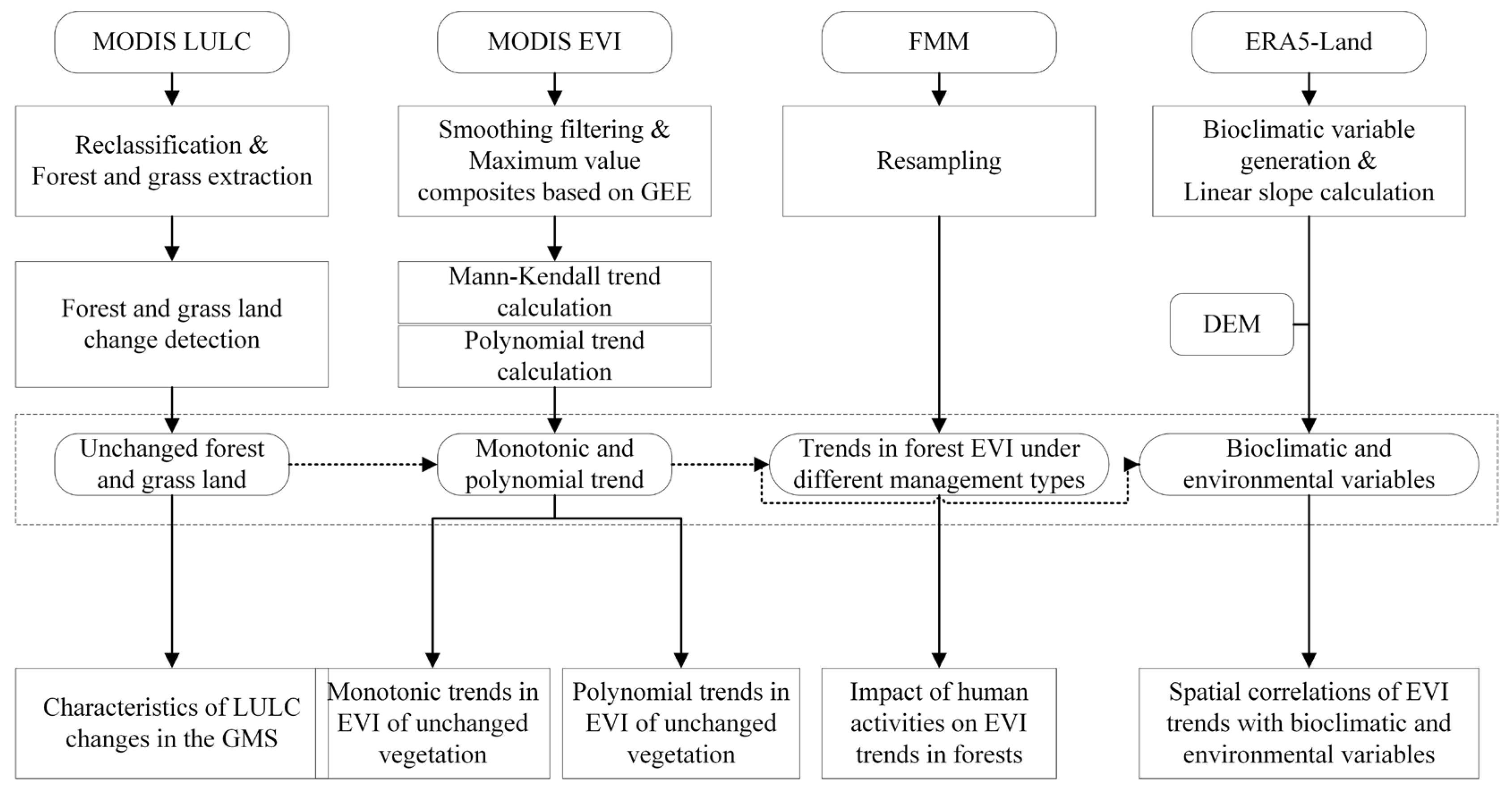
The flow of the research method is illustrated in Figure 2. After the performing pre-processing steps, such as EVI filtering, maximum value extraction, land cover reclassification, and calculation of biological variables and annual mean of net surface solar radiation, the monotonic and polynomial trends were extracted from the EVI series data. The spatial statistics were then determined. Finally, bivariate local Moran’s I (BiLISA) was used to analyze the spatial correlations between the climate and the environmental variables and EVI trends. The main steps are as follows.
(1)
Remote sensing data pre-processing
First, Savitzky Golay (S–G) filtering was performed on MODIS EVI series data from 2001 to 2020 using the Google Earth engine to remove outliers. The de-clouding of MODIS EVI was based on the labels of MODIS clouds. The maximum EVI value of each pixel was extracted from the valid EVI series data using the maximum value synthesis method [40] to obtain the E V I m a x in the ith year. The E V I m a x represented the vegetation cover and served to eliminate the influence of clouds and water vapor on the EVI and improve the reliability of the data.
In this study, the original 17 classes of MCD12Q1 were reclassified into seven classes: water bodies, forests, grasslands, croplands, cropland/natural vegetation, urban, and bare land. Evergreen needleleaf forests, evergreen broadleaf forests, deciduous needleleaf forests, deciduous broadleaf forests, mixed forests, and closed shrublands were classified as forests. Open shrublands, woody savannas, savannas, grasslands, and permanent wetlands were classified as grasslands. Permanent snow/ice and water bodies were classified as water bodies (Appendix A, Table A1).
For the ERA5-land hourly data, nine bioclimatic variables were calculated from the ERA5 land hourly data according to the definition of the “biovars” function in the “dismo” package in R 4.2.1. We then calculated the average values of five climatic variables, namely surface net solar radiation (SSR), surface solar radiation downward (SSRD), soil temperature layer 1 (STL1), volumetric soil water layer 1 (SWVl), and total evaporation (E) for 2001–2020. These data were then re-projected, cropped, and resampled into the spatial projection and resolution of MODIS EVI for subsequent data analysis. Finally, three topographic variables (elevation, slope, and aspect) were calculated using GDEMV2. These data are listed in Appendix A, Table A2.
(2)
Analysis of the EVI trend of vegetation
In this study, the Theil–Sen + Mann–Kendall (TS–MK) [41] trend analysis method was used. The TS–MK method uses Theil–Sen to calculate the trend slope and Mann–Kendall to test the significance of long time series trends. Mann–Kendall is a nonparametric statistical method widely used for the trend discrimination of meteorological and hydrological data. The Mann–Kendall method has no mandatory distribution requirements for series data and is not limited by anomalies. It is performed to statistically assess whether there is a monotonically increasing (upward) or decreasing (downward) trend in the EVI over time. A monotonically increasing trend implies that the variable increases over time. However, this trend may or may not be linear.
The Theil–Sen trend slope is calculated as follows:
β = M e d i a n ( x j x i j i )       j > i
where 1 < i < j < n , β is the slope, β > 0 indicates an upward trend in vegetation, and β < 0 indicates a downward trend in vegetation.
The statistic S for the Mann–Kendall trend test is calculated as follows:
S = i = 1 n 1 j = i + 1 n s g n ( x j x i )
where
s g n ( x j x i ) = { 1                     x j x i > 0 0                     x j x i = 0 1                   x j x i < 0  
The length of the time series in this study is n = 20 (2001–2020), and the statistic S approximately obeys the standard normal distribution. Therefore, statistic Z is used to perform the trend test, and the significance level is considered to be α = 0.05 , Z 1 α = Z 0.975 = 1.96 .
The statistic Z is calculated as follows:
Z = { S 1 V A R ( S )                         S > 0 0                                                 S = 0 S + 1 V A R ( S )                       S < 0
where
V A R ( S ) = n ( n 1 ) ( 2 n + 5 ) i = 1 m t i ( t i 1 ) ( 2 t i + 5 ) 18
where   n is the number of data points in the sequence, m is the number of knots (groups of recurring data points) in the sequence, t i is the width of the knot, that is, the number of repeated data points in the i th group of repeated datasets. A bilateral trend test was performed for the Z values. | Z | 1.96 indicates that the trend of the time series passed the significance level of 0.05.
Considering that TS–MK only detects monotonic trends, we used a polynomial trend [14] to detect nonlinear features in the EVI series data. The polynomial trend is a three-stage procedure for generating linear, quadratic, cubic, concealed, and non-trending classes of vegetation index time series. Polynomial trends are extracted using a recursive judgment method by statistically testing the significance of linear, quadratic, and cubic trends. During the first two significance tests, pixels were assigned cubic or quadratic trend classes when passing the test, but were treated as concealed classes if the slope coefficients were not statistically significant. Finally, the linear trend class was assigned to a pixel in the case of passing the significance test. Otherwise, it was regarded as having no trend.
(3)
Spatial correlation analysis of EVI trends with climate and environmental variables
To detect the spatial correlation characteristics of trends in forest EVI with bioclimatic and environmental variables, we used the BiLISA tool in GeoDa. BiLISA can reveal the spatial clustering and spatial differentiation characteristics of one attribute in each spatial cell and another attribute in the neighboring cells. BiLISA was calculated as follows:
I p q = W p q = 1 n Z p q W q
where I p q is the local spatial correlation index in spatial cells p and q , and W p and W q are the normalized values of the variance of the attribute values in spatial cells p and q, respectively. BiLISA can generate five types of spatial associations: spatially nonsignificant, high–high clustering (HH), high–low clustering (HL), low–low clustering (LL), and low–high clustering (LH). A total of nine biometeorological, two topographic, and five environmental variables were used in this study. To explore the correlation of these variables with EVI trends, we calculated their slopes for 2001–2020 using linear regression.

3. Results

3.1. Characteristics of Land Use/Land Cover Changes in the Greater Mekong Subregion

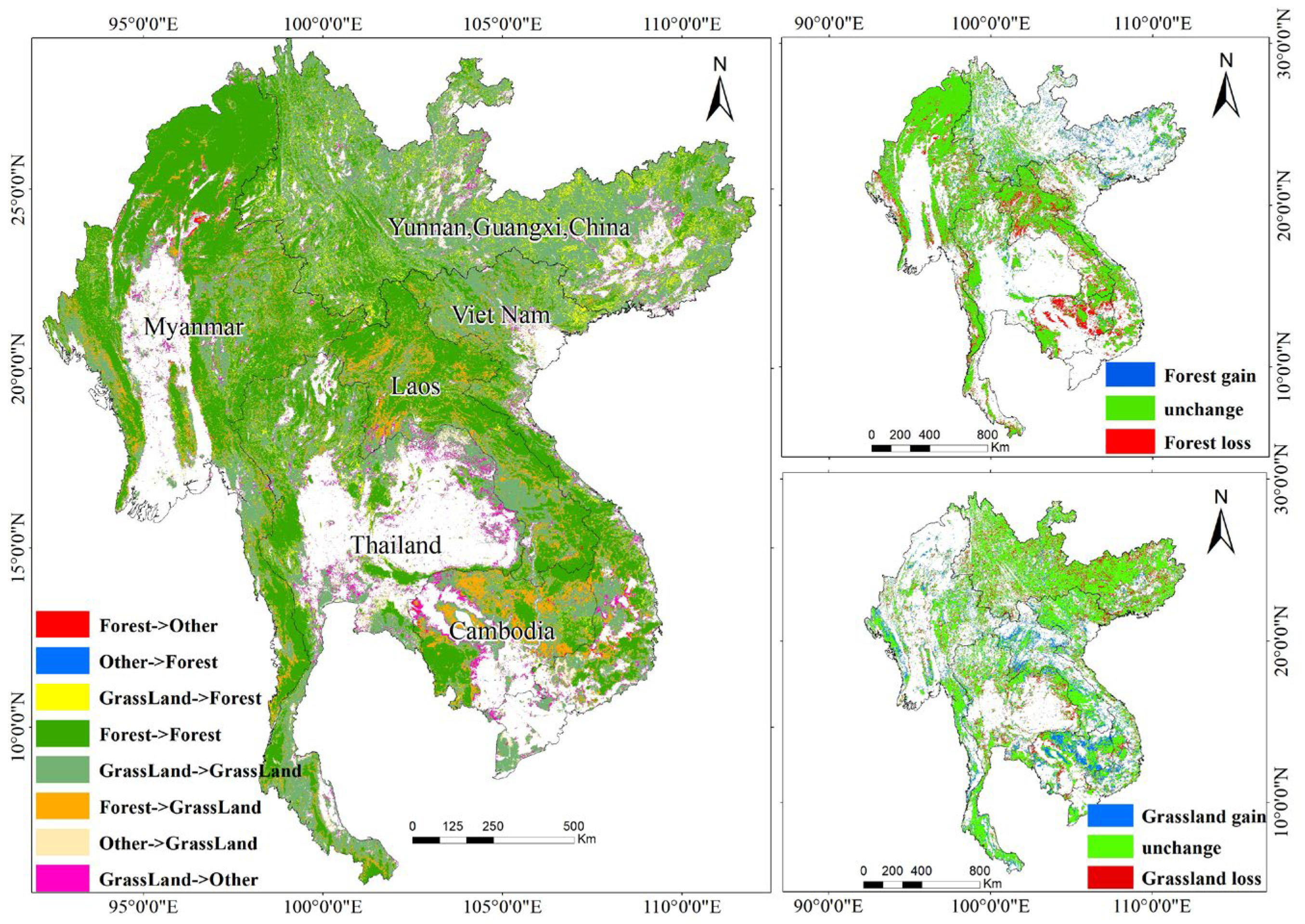
The spatial distribution of land cover of the GMS during 2001–2020 and its changes are shown in Figure 3. During 2001–2020, the land cover changes in the GMS were relatively significant, and 81.88% of the land cover types remained spatially stable. Forests and grasslands were the dominant land cover types in the GMS (Figure 3), accounting for more than 78% of the entire area. Among the categories where land cover change occurred, the pronounced ones were the conversion from forest to grassland (171,656.09 km2) and conversion from grassland to forest (114,631.71 km2). Conversion from forest to grassland was mainly distributed in Laos and Myanmar. Meanwhile, conversion from grassland to forest was mainly distributed in Guangxi and Yunnan, China, and the northern part of Thailand. In terms of forest loss and gain, Guangxi and Yunnan in China had the largest forest gain (64,036.84 km2), while Laos (3786.70 km2) and Cambodia (2695.88 km2) had the smallest gain. The largest forest loss was in Myanmar (48,560.93 km2) and the smallest was in China (14,509.18 km2). In terms of grassland loss and gain, Myanmar had the largest grassland gain (54,315.94 km2), and the remaining countries exhibited a small differences in grassland gain (33,511.51–37,695.95 km2). China had the largest grassland loss (78,044.89 km2), of which 49,281.51 km2 was transformed into forest, and the smallest grassland losses were in Laos (6636.01 km2) and Cambodia (11,674.21 km2).

3.2. Monotonic Trends in EVI of Vegetation with No Change

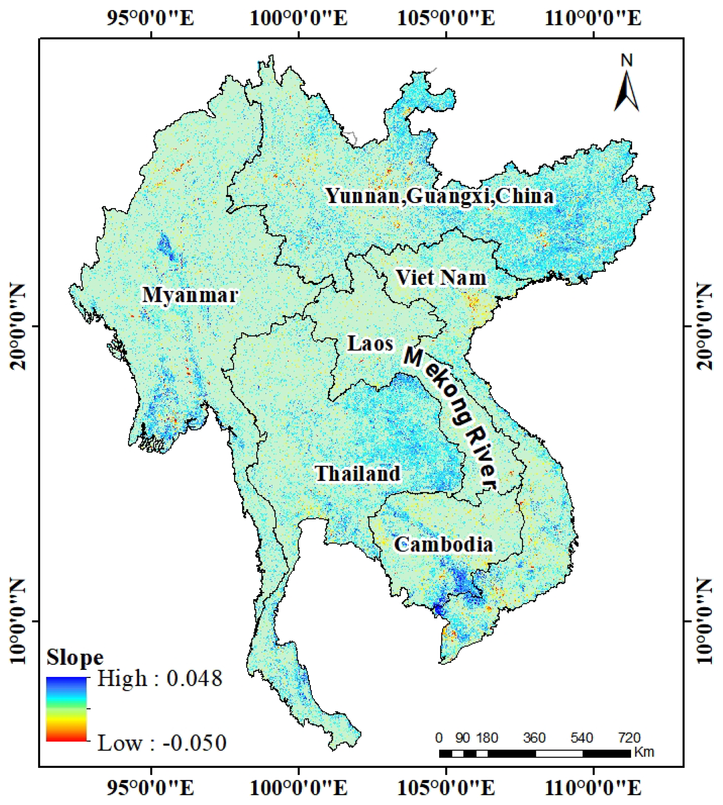
From the results of the MK significance trend test, the non-significant pixels encompassed a larger proportion of the area of each country, and were ranked according to value: Laos (89.7%) > Myanmar (83.3%) > Cambodia (74.1%) > Vietnam (73.2%) > Thailand (71.3%) > China (66.4%). Among the significant pixels, the largest proportion of the downward trend was Vietnam (5.9%), and the smallest proportion was Thailand (1.8%). In terms of the proportion of the area in an upward trend, Yunnan and Guangxi provinces in China had the largest increase (31.5%) and Laos the smallest (9.5%). Spatially (Appendix A, Figure A1), the areas with significant downward trends were mainly located around cities, such as the Red River Delta in Vietnam, Phnom Penh in Cambodia, Bangkok in Thailand, and Nanning City in Guangxi, China. The upward trend was concentrated and continuous in Guangxi Province, China, the Lower Mekong Plain, the Lower Ayeyarwady River in Myanmar, and northeastern Thailand.
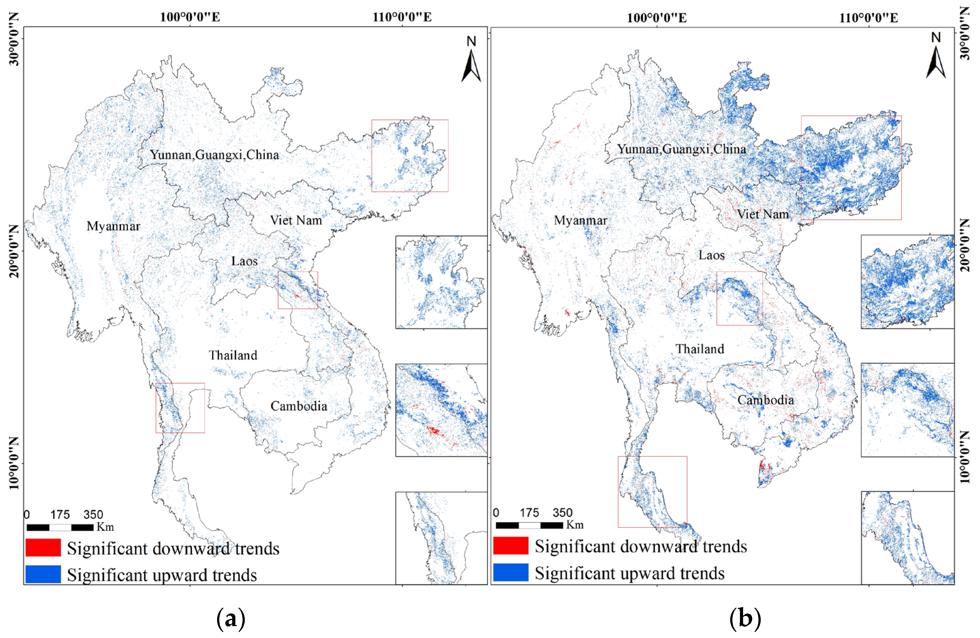
Figure 4a shows the distribution of significant trends in forest EVI without type change. Areas with a significant increase in forest EVI were located in several mountains, including the Truong Son Mountains, Birao Mountains, Arakan Mountains, and Shan Plateau as well as eastern Guangxi and southwestern Yunnan, China. Areas with a significant downward trend accounted for 8.1% of the area of the upward region and were spatially dispersed. There were also areas of intense downward movement in certain areas, such as Khammoung and Xieng Khouang in Laos. Areas with significant increases in EVI for grasslands without type change were mainly located in Guangxi and western and northern Yunnan in China, and northeastern and southern Thailand. A downward trend is present for in Laos, western Vietnam, and northern Cambodia.
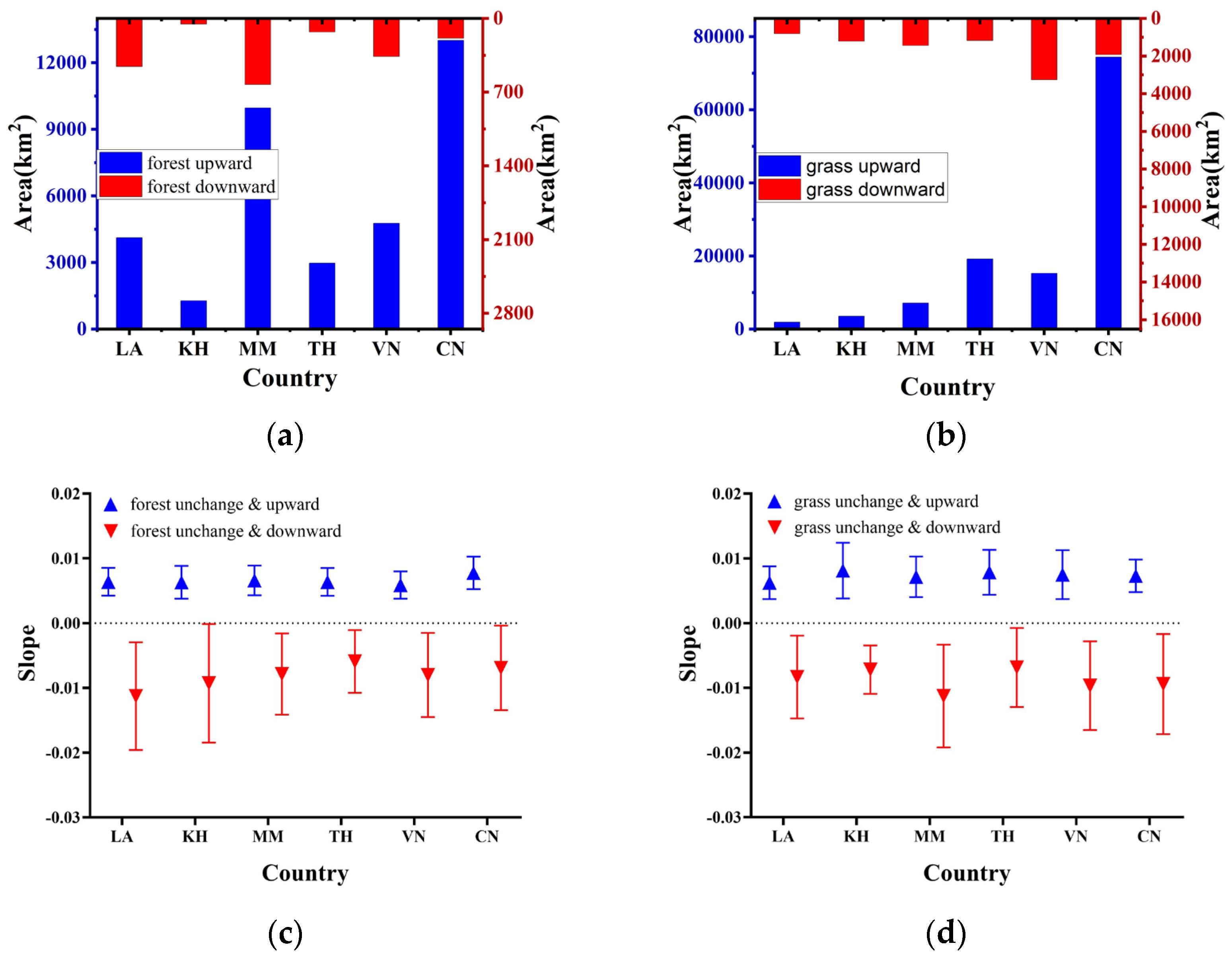
Figure 5 shows the distribution of the area and slope of the significant trend of EVI for unchanged forests and grasslands. Figure 5a shows that the largest area of significant EVI increase was in China, followed by Myanmar, and the smallest was in Cambodia. The upward trend for the EVI in the forests in each country was greater than the downward trend. For grasslands (Figure 5b), the largest area of significant EVI increase was in China and the lowest in Laos. Figure 5c,d shows the slope distribution of areas with significant EVI trends for forests and grasslands. In terms of forests, spatial variation in the slope values of forests in the GMS ranged from −0.0297 a−1 to 0.0152 a−1 over the last 20 years. For the spatial distribution, the largest upward slope was observed in China with a mean value of 0.0077 a−1, and the smallest was observed in Vietnam with a mean value of 0.0058 a−1. Dispersion of the upward slope was strongest in China and Cambodia. Meanwhile, the mean of the downward slope was more variable in the forests and more discrete than the upward trend. In terms of grasslands, the largest upward slope was for Cambodia (0.0081 a−1) and the smallest was for Laos (0.0062 a−1). The dispersion of the downward slope was greater than that of the upward slope. In summary, the overall trend for forests and vegetation without type change in the last 20 years in the GMS was upward.

3.3. Polynomial Trends in EVI of Vegetation with No Change

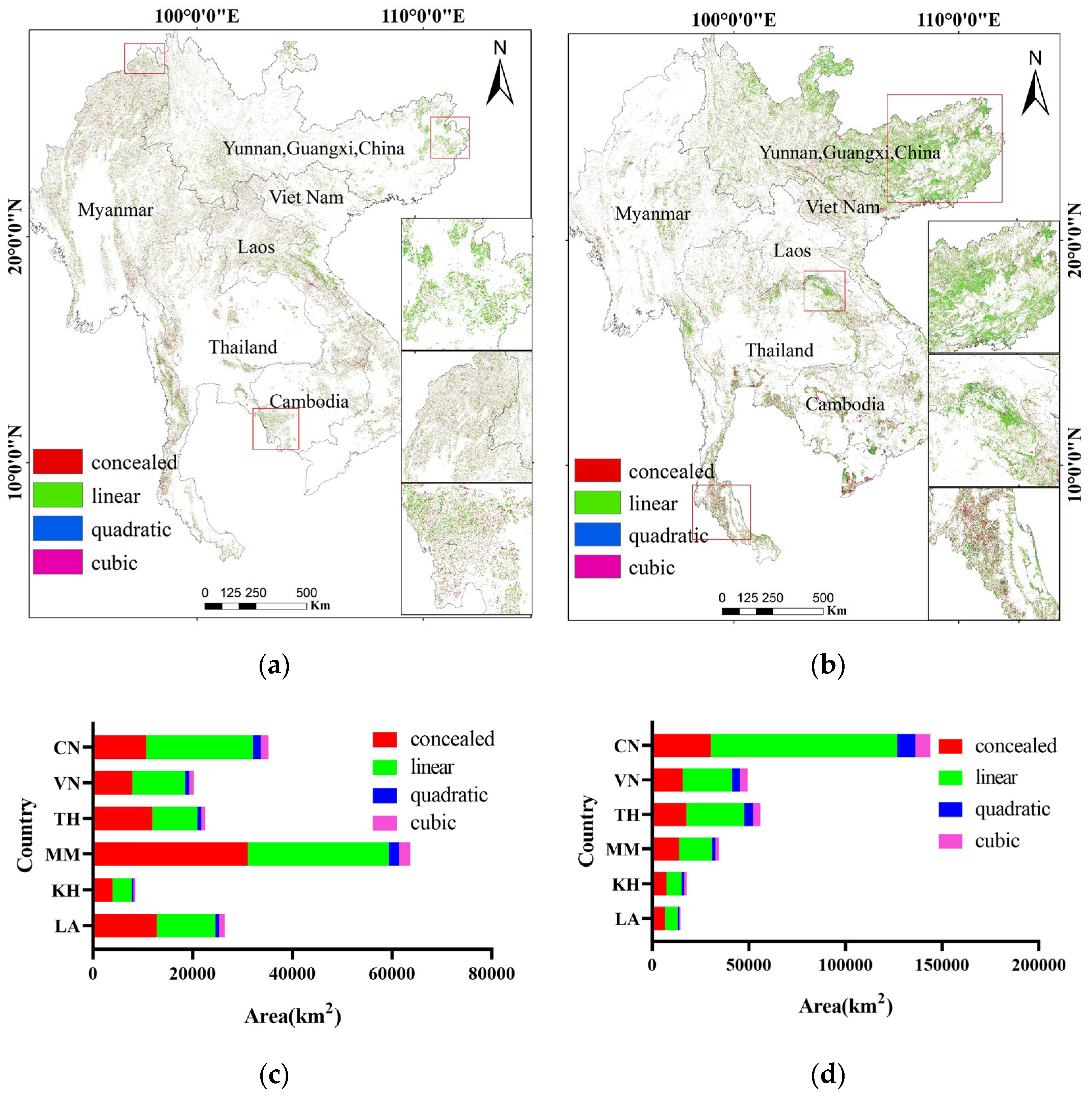
We extracted polynomial trends for forests and grasslands that had not experienced type changes (Figure 6). Five types of results were included in the polynomial trend algorithm, namely linear, quadratic, cubic, concealed trend, and no-trend classes. Only the first four types are presented here. Figure 6a shows the polynomial trends of the forests over the last 20 years. Spatially, the polynomial trends for forests were concentrated in the Shan Plateau, Arakan Mountains, Birao Mountains, Xieng Khouang Plateau, and lower and middle Mekong Mountains. Concealed forest trends were widely distributed and dispersed. Linear trends in forests were mainly observed in Ha Tinh Province and the Birao Mountains in Vietnam, the Cardamom Mountains in Cambodia, and the eastern and southern parts of Guangxi, China. Meanwhile, dispersed linear trends were observed in the Shan Plateau in northern Myanmar and the Hengduan Mountains in Yunnan. Quadratic and cubic trends were not spatially significant. Figure 6c shows that the forest had the largest proportion of concealed trends in terms of area, followed by linear trends, while the proportion of quadratic and cubic trends was smaller. Among the six countries, the concealed and linear trends were the largest in Myanmar. In China, the largest proportion of linear trends were found in forests, followed by concealed trends. Cambodia had the smallest area for all trends. In terms of grasslands, linear trends were mainly distributed in the eastern part of the Korat Plateau and the southern part of Changwat Krabi in Thailand, Guangxi province and the eastern part of Yunnan province in China, and Mon State in Myanmar (Figure 6b). The concealed, quadratic, and cubic trends were spatially dispersed, with only the quadratic trend being more concentrated in the northern part of Ho Chi Minh City in Vietnam. Figure 6d shows the area proportion for each trend. Compared with forests, the linear trend was larger in grasslands, followed by concealed trends. There was little difference in the proportions of quadratic and cubic trends for grasslands among the six countries.
Compared to TS–MK (Figure 5), the polynomial trend method (Figure 6) can detect more pixels with trends. In terms of forests, 11.28% of the pixels that did not show a significant trend in TS–MK were judged as concealed trend classes by polynomial trends, and 3.02% of the pixels were judged as linear (2.49%), quadratic (0.25%), and cubic (0.28%) trend classes. In pixels with TS–MK upward trends, the percentages of concealed, linear, quadratic, and cubic trend classes were 2.07%, 68.56%, 4.48%, and 4.8%, respectively. For the pixels with TS–MK downward trends, the percentages of concealed, linear, quadratic, and cubic trend classes were 2.92%, 58.69%, 6.4%, and 8.7%, respectively. With grasslands, the polynomial trend determined the pixels in which the TS–MK method showed no significant trend as concealed (14.74%), linear (3.5%), quadratic (0.62%), and cubic (0.49%) trend classes. The percentage of linear, quadratic, and cubic trend classes was higher than that of the forest in pixels with TS–MK upward and downward trends, whereas the percentage of concealed trends was lower than that of forests.

3.4. Impact of Human Activities on EVI Trends in Forests

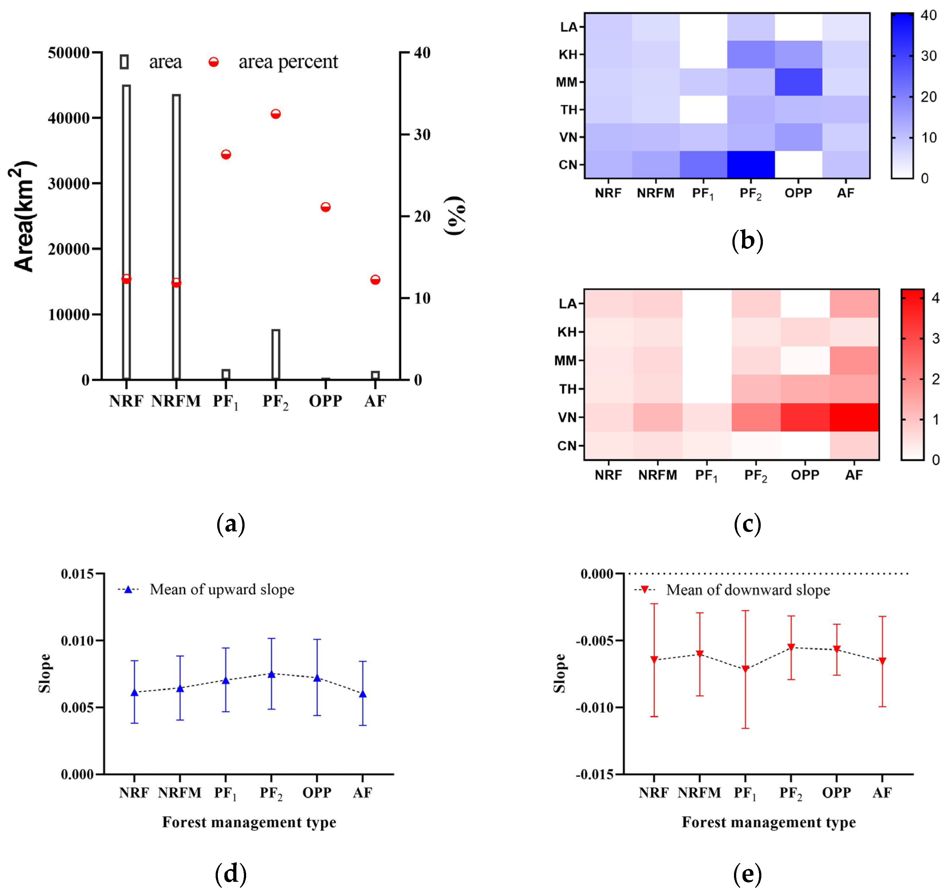
Figure 7a shows the distribution of significant trends in EVI for the forest management types defined by the FMM and the proportion of their area in each category. The areas of NRF and NRFM areas were the largest in the GMS. The proportion of significant trends was the largest in PF2 and PF1. This indicates that anthropogenic activities in the GMS strongly influence significant changes in forest EVI. For each country, Figure 7b,c shows the proportions of upward and downward trends in EVI for each forest management class. In terms of upward trends (Figure 7b), PF1 and PF2 had the largest proportions in China, reaching 27.76% and 40.46%, respectively, whereas AF had the lowest (9.53%). In Vietnam, the OPP had the largest upward trend, whereas the AP had the smallest. In Thailand, PF2 showed the largest upward trend and NFRM the smallest. In Myanmar, the OPP showed the largest upward trend and the AP the smallest. In Cambodia, PF2 showed the largest upward trend and NFRM the smallest. Overall, China showed relatively high upward trends in NRF, NRFM, PF1, and PF2, whereas other countries showed high upward trends in PF2 and OPP. As shown in Figure 7c, Vietnam showed the most pronounced downward trends in PF2 (2.11%), OPP (3.46%), and AF (4.22%), while other countries showed the largest proportion of downward trends in AF. However, the downward trend in GMS forests affected a small proportion (ranging from 0.36% to 4.2%). Figure 7d,e show the slope of the significant trend in EVI for different forest management types. In the upward trends, the PF2 of GMS showed the largest variation ( 0.0075 ± 0.0027 ), and the smallest was AF ( 0.0060 ± 0.0023 ). For the downward trends, PF1 had the highest variation ( 0.0071 ± 0.0044 ), and its dispersion was larger. PF2 exhibited the smallest variation ( 0.0055 ± 0.0023 ).

3.5. Spatial Correlation Analysis of Trends in EVI with Climate and Environmental Variables

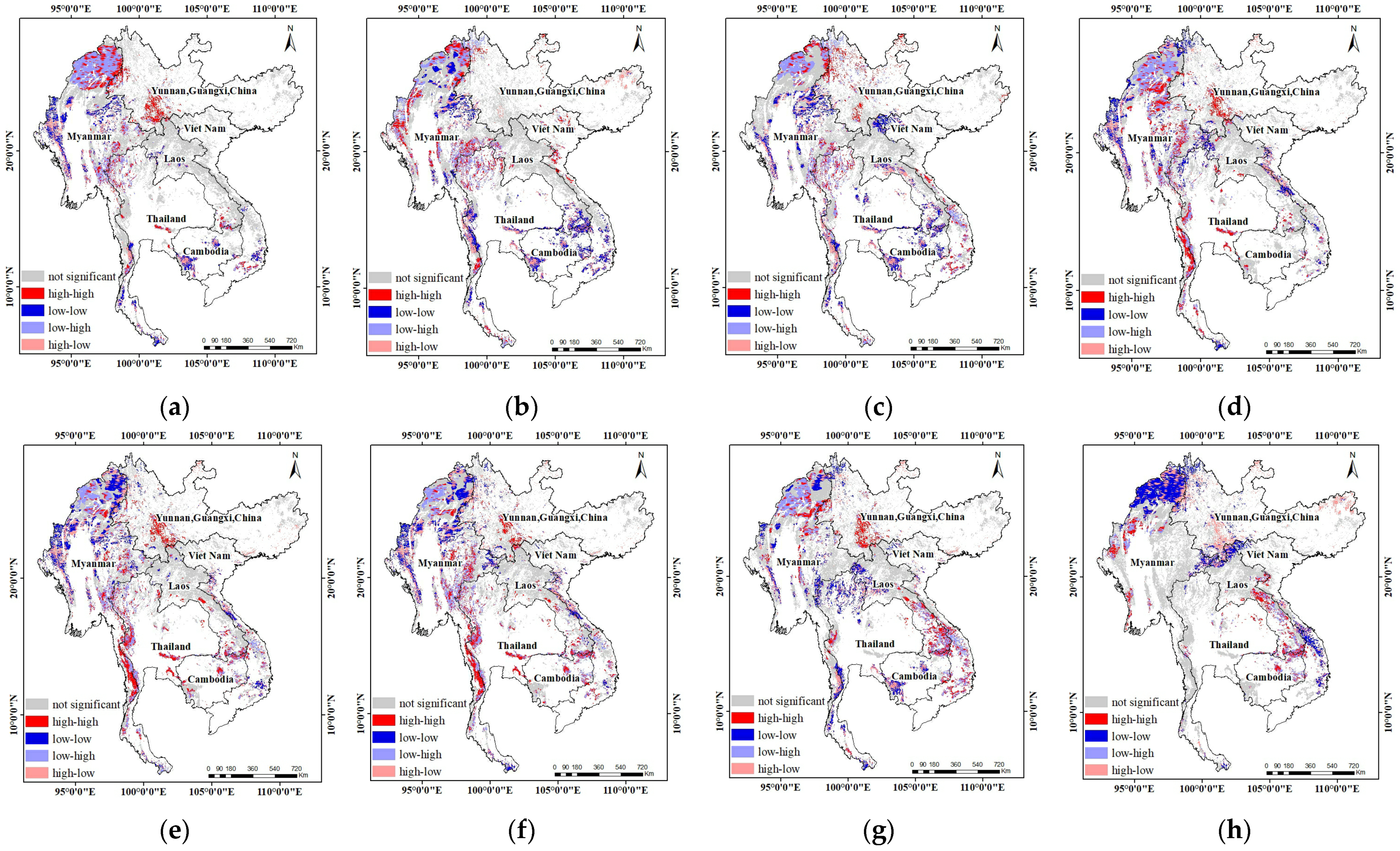
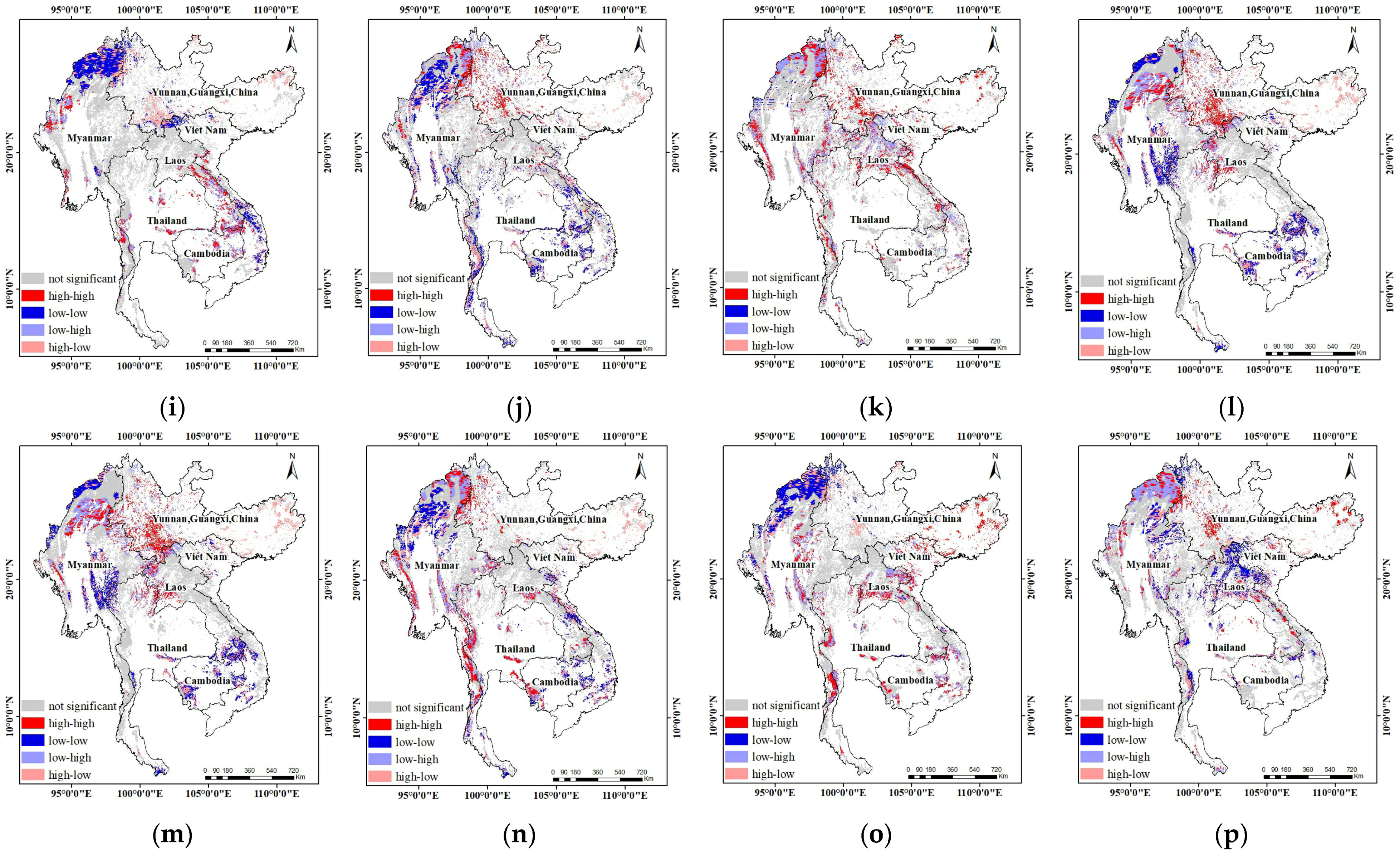
Overall, among the 16 variables, the average percentage of those without significant clustering characteristics with forest EVI trends reached 60.37%. Meanwhile, among those with significant clustering characteristics with forest EVI trends (p < 0.05), the average percentages of high–high clustering (HH), low–low clustering (LL), low–high clustering (LH), and high–low clustering (HL) were 9.56%, 9.86%, 11.02%, and 9.19%, respectively. In terms of clustering characteristics, the largest percentage of EVI with no significant characteristics was observed for bio01 (67.25%) and the smallest for SSR (51.24%). In HH clustering, the largest proportion was observed for EVI with a topographic slope (15.15%) and the smallest in bio12 (3.47%). In LL clustering, the largest proportion was observed for EVI with elevation (15.61%) and the smallest for topographic slope (1.50%). In LH clustering, the largest proportion was observed for EVI with a topographic slope (16.29%) and the smallest with bio12 (6.93%). In the HL clustering, the largest proportion was obtained for EVI with elevation (13.59%) and the smallest with topographic slope (1.19%). Spatially, LL clustering was most evident in the northern part of Myanmar, as shown in Figure 8e,g–j,o. LL clustering also exists in transnational regions, such as the borders of China, Vietnam and Laos, as shown in Figure 8c,h,i,p, and the borders of Vietnam, Laos and Cambodia, as shown in Figure 8b,j,l,m. LH clustering is mainly present in the northern part of Myanmar, as shown in Figure 8a–g,p. HL clustering was most evident in Yunnan and Guangxi, China, and Myanmar, as shown in Figure 8a,c–f,h–n. HH clustering was mainly distributed in northern Myanmar and southern Yunnan, China (Figure 8a,d,e,g,j–m,p), central Truong Son Mountains of Laos and Vietnam (Figure 8g–i,k), and the Birao Mountains of Myanmar and southern Thailand (Figure 8b,d–f,n,o).

4. Discussion

Overall, our results showed (Figure 3) that forests were decreasing in five of the six GMS countries, with Laos and Cambodia showing the largest reductions over the last 20 years. Meanwhile, China was the only country with an increase in the forest area. According to Tölle [42], forest dynamics occurred in stages, with a sharp decrease in forest area after 2000, which continued until 2018, as in Cambodia and Vietnam. In recent years, some countries have shown signs of reforestation or slow deforestation, such as Thailand [43,44]. According to food and agriculture organization studies, the recovery of forest cover in some countries is attributed to the expansion of plantations [45,46]. Therefore, despite the general slowdown in deforestation and efforts to increase forests in these countries, the trend of tropical forest decline has not changed [47]. Much of this forest decline has shifted to grasslands, as seen in southern Cambodia and northern Laos (Figure 3). These declines occurred in the marginal parts of forested areas, which is consistent with the trend observed by Tölle [42]. Land policies in China have been adjusted in recent years. In Guangxi, during the Tenth Five-Year Plan, forestry projects included the return of cultivated land to forest, the construction of fast-growing and productive forest bases, and the construction of nature reserves, Pearl River protection forests, and coastal protection forests [48]. Open forest land with 10–30% depression and high-cover grassland with >50% cover were planted into timber and economic forests [49]. This is the main anthropogenic factor affecting forest growth in China.
In recent years, global vegetation is becoming greener [50], including in India, southern and southeastern China, and Southeast Asia [51]. Study timespans are important for determining time-series trends in vegetation indices [16]. It has been shown that global vegetation trends after 2000 are highly uncertain [47]. Multiple trend detection methods are required to assess the coherence of trends. In this study, a monotonic trend assessment method and polynomial trend analysis were used. With TS–MK, the polynomial trend was able to find more trend pixels in EVI, especially those with concealed trends. In contrast, 58.69–68.56% of the significant trend pixels were linear. This does not mean that TS–MK overestimated the trend variation of the EVI. The TS–MK method is insensitive to noise, does not require the data to obey a normal distribution, and has high reliability in monotonic trend detection. The difference in the number of linear trends may be attributed to the polynomial trend that assigns pixels from the monotonic trend to the quadratic and cubic trend classes. In terms of spatial distribution, the trends were similar. In the case of forests, areas where trends were clearly concentrated were distributed in eastern China and central Laos. Meanwhile, areas where trends appeared more dispersed were distributed in the mountainous areas between Myanmar and Yunnan, China. The similarity in spatial distribution characteristics of the results of the two detection methods was more evident in grassland trend maps. From the results of vegetation index trends, all six countries located in the study area had unique land use policies, and therefore, may have unique vegetation trend trajectories. Chen et al. [47] showed that the “greening” of Earth is mainly attributed to increasing in human agriculture and forest replanting. In this study, we excluded agriculture and areas where forest categories changed over a 20-year period. As shown in Figure 5 and Figure 6, these increasing trends in EVI were significantly greater than the decreasing trends. However, spatially, the increasing and decreasing trends in EVI are intertwined, which is consistent with the observations of Chen [51].
In terms of land cover change, the GMS had the greatest reduction in forests, and the greatest increase in grasslands (Figure 3), and a large proportion of conversion from forests to grasslands. One of the main driving factors is deforestation by agricultural production in Southeast Asian countries [52]. The high value of forests to the ecology of the GMS and the sustainability of human society is well known. Therefore, this study used BiLISA to analyze the spatial clustering characteristics of biometeorological and topographic factors and forest EVI trends. From the results, 16 variables with no significant spatial correlation with forest EVI trends in the GMS accounted for most of this region. Net surface solar radiation (SSR; 12.19%), downward surface solar radiation, (SSRD; 12.14%), and elevation (11.29%) were the three variables with the largest average distribution correlated with EVI trends (HH, LL, LH, and HL). This was followed by STL1 (soil temperature class 1, 10.52%), Bio05 (maximum temperature in the warmest month, 10.47%), Bio09 (average temperature in the driest quarter, 10.36%), and Bio08 (average temperature in the wettest quarter, 10.26%) in the biometeorological variables, although the differences in the average proportions between them were relatively small. The smallest average proportions of spatial clustering characteristics with EVI trends were the topographic slope (8.53%), Bio15 (precipitation seasonality, 8.33%), and Bio01 (annual mean temperature, 8.19%). Nemani [20] suggested that vegetation growth in Southeast Asia is mainly limited by radiation rather than by other climatic factors such as precipitation and temperature. Results of our BiLISA analysis also showed that radiation (SSR and SSRD) had the largest spatial correlation with forest EVI trends. In addition, forest EVI trends were also influenced by elevation due to differences in hydrothermal, light, and atmospheric conditions resulting from different elevations. Our results further confirmed that the precipitation and temperature variables Bio15 and Bio01 were the two variables with the lowest spatial correlation with forest EVI trends; however, seasonal changes in precipitation and temperature were more spatially correlated with forest EVI trends.
To date, we have only analyzed monotonic and polynomial trends, which complicated determining of the response of vegetation to weather extremes. In future studies, we will use long-term time-series datasets to capture trends and their turning points as well as related influencing factors. In this study, we analyzed anthropogenic activities in unchanged forest areas. Considering the higher anthropogenic activities in the GMS, the impacts of anthropogenic activities on other vegetation types will be further explored.

5. Conclusions

This study aimed to analyze the change characteristics of land cover as well as grassland and forest EVI of six countries in the GMS, and their spatial correlation with bioclimatic and environmental variables. We used TS–MK and polynomial regression to extract the vegetation trends in MODIS EVI over the past 20 years, and BiLISA was used to characterize the spatial clustering of bioclimatic and environmental variables with forest EVI trends. The results of the study show that land cover changes in the GMS were relatively large during 2001–2020. Among types of land cover change, conversion between forest and grassland was the main trend. The EVI trend in forests and grasslands without a type change in the GMS was upward. Forest EVI trends in the six countries were strongly influenced by anthropogenic activities, especially planted forests and plantation forests in China, and oil palm plantations in the other countries. Changes in forest EVI were most spatially correlated with radiation and least spatially correlated with the seasonality of precipitation and mean annual temperature. Considering the relatively high population density and unbalanced economic development in the GMS, the sustainable development of society is urgently needed for soil and water conservation, carbon sequestration capacity, and protecting the economic value of forests. While working towards, regional economic development, countries should work together to strengthen the regulation of anthropological activities and effectively reduce forest loss.

Author Contributions

Conceptualization, B.H. and X.W.; Data curation, K.L. and W.Z.; Formal analysis, B.H.; Funding acquisition, B.H. and K.L.; Investigation, B.H. and W.C.; Methodology, B.H.; Project administration, B.H.; Resources, B.H.; Software, K.L.; Supervision, B.H.; Validation, B.H. and Y.Y.; Visualization, K.L.; Writing—original draft, B.H. and X.W.; Writing—review and editing, B.H. and K.L. All authors have read and agreed to the published version of the manuscript.

Funding

This research was funded by the National Key Research and Development Program of China (No. 2022YFB3904203), the Shenzhen Fundamental Research Program (No. JCYJ20190812171419161, JCYJ20190807163001783).

Data Availability Statement

The MODIS EVI and MCD12C1 data sets are available from https://code.earthengine.google.com (accessed on 12 February 2022). The ERA5-LAND are available from https://cds.climate.copernicus.eu/cdsapp#!/dataset/reanalysis-era5-land?tab=form (accessed on 14 February 2022). The ASTER GDEM V2 are available from http://www.gscloud.cn/ (accessed on 14 February 2022). The globally consistent forest management map data are available from https://doi.org/10.5281/zenodo.5879022 (accessed on 14 February 2022).

Conflicts of Interest

The authors declare no conflict of interest.

Appendix A

Table A1. MODIS land cover reclassification.
ClassesCodeReclassified ClassesNew Code
Evergreen needleleaf forests1Forests1
Evergreen broadleaf forests2
Deciduous needleleaf forests3
Deciduous broadleaf forests4
Mixed forests5
Closed shrublands6
Open shrublands7Grasslands2
Woody savannas8
Savannas9
Grasslands10
Permanent wetlands11
Croplands12Croplands3
Urban and built-up lands13Urban and Built-up Lands4
Cropland/natural vegetation mosaics14Cropland/Natural Vegetation Mosaics5
Barren15Barren6
Permanent snow and ice16Water Bodies7
Water bodies17
Unclassified255Unclassified
Table A2. Biometeorological and topographic factors.
VariableCodeUnit
Annual mean temperaturebio01°C/a
Temperature seasonalitybio04°C/a
Max Temperature of warmest monthbio05°C/a
Min temperature of the coldest monthbio06°C/a
Mean temperature of wettest quarterbio08°C/a
Mean temperature of driest quarterbio09°C/a
Mean temperature of warmest quarterbio10°C/a
Annual precipitationbio12mm/a
Precipitation seasonalitybio15%/a
Elevationelevationm
Topographic Slopeslope°C
Surface net solar radiationssrJ m−2
Surface solar radiation downwardsssrdJ m−2
Soil temperature level 1stl1K
Volumetric soil water layer 1swvl1m3
Total evaporationem of water equivalent
Figure A1. Map of the monotonic trend slope in GMS.
Remotesensing 14 05982 g0a1

References

  1. Qu, L.; Huang, Y.; Yang, L.; Li, Y. Vegetation restoration in response to climatic and anthropogenic changes in the Loess Plateau, China. Chin. Geogr. Sci. 2020, 30, 89–100. [Google Scholar] [CrossRef] [Green Version]
  2. Wang, H.; Yan, S.; Liang, Z.; Jiao, K.; Li, D.; Wei, F.; Li, S. Strength of association between vegetation greenness and its drivers across China between 1982 and 2015: Regional differences and temporal variations. Ecol. Indic. 2021, 128, 107831. [Google Scholar] [CrossRef]
  3. Fensholt, R.; Rasmussen, K.; Nielsen, T.T.; Mbow, C. Evaluation of earth observation based long term vegetation trends- Intercomparing NDVI time series trend analysis consistency of Sahel from AVHRR GIMMS, Terra MODIS and SPOT VGT data. Remote Sens. Environ. 2009, 113, 1886–1898. [Google Scholar] [CrossRef]
  4. Tian, F.; Brandt, M.; Liu, Y.Y.; Verger, A.; Tagesson, T.; Diouf, A.A.; Rasmussen, K.; Mbow, C.; Wang, Y.; Fensholt, R. Remote sensing of vegetation dynamics in drylands: Evaluating vegetation optical depth (VOD) using AVHRR NDVI and in situ green biomass data over West African Sahel. Remote Sens. Environ. 2016, 177, 265–276. [Google Scholar] [CrossRef] [Green Version]
  5. Mangiarotti, S.; Mazzega, P.; Hiernaux, P.; Mougin, M. The vegetation cycle in West Africa from AVHRR–NDVI data: Horizons of predictability versus spatial scales. Remote Sens. Environ. 2010, 114, 2036–2047. [Google Scholar] [CrossRef] [Green Version]
  6. Setiawan, Y.; Yoshino, K.; Prasetyo, L.B. Characterizing the dynamics change of vegetation cover on tropical forestlands using 250 m multi-temporal MODIS EVI. Int. J. Appl. Earth Obs. Geoinf. 2014, 26, 132–144. [Google Scholar] [CrossRef]
  7. Zhang, Y.; Song, C.; Band, L.E.; Sun, G.; Li, J. Reanalysis of global terrestrial vegetation trends from MODIS products: Browning or greening? Remote Sens. Environ. Inter. Dis. J. 2017, 191, 145–155. [Google Scholar] [CrossRef] [Green Version]
  8. Huete, A.; Didan, K.; Miura, T.; Rodriguez, E.P.; Gao, X.; Ferreira, L.G. Overview of the radiometric and biophysical performance of the MODIS vegetation indices. Remote Sens. Environ. 2002, 83, 195–213. [Google Scholar] [CrossRef]
  9. Qiu, B.; Zhong, J.; Tang, Z.; Feng, M.; Chen, C.; Wang, X. Greater phenological sensitivity on the higher Tibetan Plateau: New insights from weekly 5 km EVI2 datasets. Int. J. Biometeorol. 2016, 61, 807–820. [Google Scholar] [CrossRef] [PubMed]
  10. Jiang, M.; He, Y.; Song, C.; Pan, Y.; Qiu, T.; Tian, S. Disaggregating climatic and anthropogenic influences on vegetation changes in Beijing-Tianjin-Hebei region of China. Sci. Total Environ. 2021, 786, 147574. [Google Scholar] [CrossRef]
  11. Santana, R.O.; Delgado, R.C.; Schiavetti, A. The past, present and future of vegetation in the Central Atlantic Forest Corridor, Brazil. Remote Sens. Appl. Soc. Environ. 2020, 20, 100357. [Google Scholar] [CrossRef]
  12. Ren, Z.; Tian, Z.; Wei, H.; Liu, Y.; Yu, Y. Spatiotemporal evolution and driving mechanisms of vegetation in the Yellow River Basin, China during 2000–2020. Ecol. Indic. 2022, 138, 108832. [Google Scholar] [CrossRef]
  13. Ju, J.; Masek, J.G. The vegetation greenness trend in Canada and US Alaska from 1984–2012 Landsat data. Remote Sens. Environ. Inter. Dis. J. 2016, 176, 1–16. [Google Scholar] [CrossRef]
  14. Jamali, S.; Seaquist, J.; Eklundh, L.; Ardö, J. Automated mapping of vegetation trends with polynomials using NDVI imagery over the Sahel. Remote Sens. Environ. 2014, 141, 79–89. [Google Scholar] [CrossRef]
  15. de Jong, R.; Verbesselt, J.; Schaepman, M.E.; de Bruin, S. Trend changes in global greening and browning: Contribution of short-term trends to longer-term change. Glob. Chang. Biol. 2012, 18, 642–655. [Google Scholar] [CrossRef]
  16. Piao, S.; Wang, X.; Ciais, P.; Zhu, B.; Wang, T.; Liu, J. Changes in satellite-derived vegetation growth trend in temperate and boreal Eurasia from 1982 to 2006. Glob. Chang. Biol. 2011, 17, 3228–3239. [Google Scholar] [CrossRef]
  17. Verbesselt, J.; Hyndman, R.; Zeileis, A.; Culvenor, D. Phenological change detection while accounting for abrupt and gradual trends in satellite image time series. Remote Sens. Environ. 2010, 114, 2970–2980. [Google Scholar] [CrossRef] [Green Version]
  18. Jamali, S.; Jönsson, P.; Eklundh, L.; Ardö, J.; Seaquist, J. Detecting changes in vegetation trends using time series segmentation. Remote Sens. Environ. 2015, 156, 182–195. [Google Scholar] [CrossRef]
  19. Pan, N.; Feng, X.; Fu, B.; Wang, S.; Ji, F.; Pan, S. Increasing global vegetation browning hidden in overall vegetation greening: Insights from time-varying trends. Remote Sens. Environ. 2018, 214, 59–72. [Google Scholar] [CrossRef]
  20. Nemani, R.R.; Keeling, C.D.; Hashimoto, H.; Jolly, W.M.; Piper, S.C.; Tucker, C.J.; Myneni, R.B.; Running, S.W. Climate-driven increases in global terrestrial net primary production from 1982 to 1999. Science 2003, 300, 1560–1563. [Google Scholar] [CrossRef] [PubMed]
  21. Wu, Y.; Tang, G.; Gu, H.; Liu, Y.; Yang, M.; Sun, L. The variation of vegetation greenness and underlying mechanisms in Guangdong province of China during 2001–2013 based on MODIS data. Sci. Total Environ. 2019, 653, 536–546. [Google Scholar] [CrossRef] [PubMed]
  22. Piao, S.; Yin, G.; Tan, J.; Cheng, L.; Huang, M.; Li, Y.; Liu, R.; Mao, J.; Myneni, R.B.; Peng, S.; et al. Detection and attribution of vegetation greening trend in China over the last 30 years. Glob. Chang. Biol. 2015, 21, 1601–1609. [Google Scholar] [CrossRef] [PubMed]
  23. Kalisa, W.; Igbawua, T.; Henchiri, M.; Ali, S.; Zhang, S.; Bai, Y.; Zhang, J. Assessment of climate impact on vegetation dynamics over East Africa from 1982 to 2015. Sci. Rep. 2019, 9, 16865. [Google Scholar] [CrossRef] [PubMed] [Green Version]
  24. Gao, M.; Piao, S.; Chen, A.; Yang, H.; Liu, Q.; Fu, Y.H.; Janssens, I.A. Divergent changes in the elevational gradient of vegetation activities over the last 30 years. Nat. Commun. 2019, 10, 2970. [Google Scholar] [CrossRef] [PubMed] [Green Version]
  25. Lamchin, M.; Lee, W.K.; Jeon, S.W.; Wang, S.W.; Lim, C.H.; Song, C.; Sung, M. Long-term trend and correlation between vegetation greenness and climate variables in Asia based on satellite data. Sci. Total Environ. 2018, 618, 1089–1095. [Google Scholar] [CrossRef]
  26. Piao, S.; Nan, H.; Huntingford, C.; Ciais, P.; Friedlingstein, P.; Sitch, S.; Peng, S.; Ahlström, A.; Canadell, J.G.; Cong, N.; et al. Evidence for a weakening relationship between interannual temperature variability and northern vegetation activity. Nat. Commun. 2014, 5, 5018. [Google Scholar] [CrossRef] [PubMed] [Green Version]
  27. Xu, X.; Liu, H.; Jiao, F.; Gong, H.; Lin, Z. Nonlinear relationship of greening and shifts from greening to browning in vegetation with nature and human factors along the Silk Road Economic Belt. Sci. Total Environ. 2021, 766, 142553. [Google Scholar] [CrossRef]
  28. Chu, H.; Venevsky, S.; Chao, W.; Wang, M. NDVI-based vegetation dynamics and its response to climate changes at Amur-Heilongjiang River Basin from 1982 to 2015. Sci. Total Environ. 2019, 650, 2051–2062. [Google Scholar] [CrossRef] [PubMed]
  29. Zhao, C.; Yan, Y.; Ma, W.; Shang, X.; Cheng, J.; Rong, Y.; Xie, T.; Quan, Y. RESTREND-based assessment of factors affecting vegetation dynamics on the Mongolian Plateau. Ecol. Model. 2021, 440, 109415. [Google Scholar] [CrossRef]
  30. Evans, J.; Geerken, R. Discrimination between climate and human-induced dryland degradation. J. Arid Environ. 2004, 57, 535–554. [Google Scholar] [CrossRef]
  31. Wessels, K.J.; Prince, S.D.; Malherbe, J.; Small, J.; Frost, P.; VanZyl, D. Can human-induced land degradation be distinguished from the effects of rainfall variability? A case study in South Africa. J. Arid Environ. 2007, 68, 271–297. [Google Scholar] [CrossRef]
  32. Wessels, K.J.; den Bergh, F.; Scholes, R.J. Limits to detectability of land degradation by trend analysis of vegetation index data. Remote Sens. Environ. 2012, 125, 10–22. [Google Scholar] [CrossRef]
  33. Fang, J.; Song, Y.; Liu, H.; Piao, S. Vegetation-climate relationship and its application in the division of vegetation zone in China. Acta Bot. Sin. 2002, 44, 1105–1122. [Google Scholar]
  34. Zhang, Y.; Zhu, Z.; Liu, Z.; Zeng, Z.; Ciais, P.; Huang, M.; Liu, Y.; Piao, S. Seasonal and interannual changes in vegetation activity of tropical forests in Southeast Asia. Agric. For. Meteorol. 2016, 224, 1–10. [Google Scholar] [CrossRef]
  35. Wu, J.; Wang, X.; Zhong, B.; Yang, A.; Jue, K.; Wu, J.; Zhang, L.; Xu, W.; Wu, S.; Zhang, N.; et al. Ecological environment assessment for Greater Mekong Subregion based on Pressure-State-Response framework by remote sensing. Ecol. Indic. 2020, 117, 106521. [Google Scholar] [CrossRef]
  36. WWF. First Contact in the Greater Mekong: New Species Discoveries. Available online: https://www.worldwildlife.org/publications/first-contact-in-the-greater-mekong-new-species-discoveries (accessed on 5 December 2021).
  37. ECMWF. ERA5-Land: Data Documentation. Available online: https://confluence.ecmwf.int/display/CKB/ERA5-Land%3A+data+documentation (accessed on 5 December 2021).
  38. Geospatial Data Cloud. Available online: http://www.gscloud.cn/ (accessed on 5 December 2021).
  39. Lesiv, M.; Schepaschenko, D.; Buchhorn, M.; See, L.; Dürauer, M.; Georgieva, I.; Jung, M.; Hofhansl, F.; Schulze, K.; Bilous, A.; et al. Global forest management data for 2015 at a 100 m resolution. Sci. Data 2022, 9, 199. [Google Scholar] [CrossRef] [PubMed]
  40. Holben, B.N. Characteristics of maximum-value composite images from temporal AVHRR data. Int. J. Remote Sens. 1986, 7, 1417–1434. [Google Scholar] [CrossRef]
  41. Yao, R.; Wang, L.; Huang, X.; Chen, X.; Liu, Z. Increased spatial heterogeneity in vegetation greenness due to vegetation greening in mainland China. Ecol. Indic. 2019, 99, 240–250. [Google Scholar] [CrossRef]
  42. Tölle, M.H.; Engler, S.; Panitz, H.J. Impact of Abrupt Land Cover Changes by Tropical Deforestation on Southeast Asian Climate and Agriculture. J. Clim. 2017, 30, 2587–2600. [Google Scholar] [CrossRef]
  43. FAO. Southeast Asian Forests and Forestry to 2020. 2011. Available online: http://www.fao.org/3/i1964e/i1964e00.htm (accessed on 11 December 2021).
  44. Boori, M.S.; Choudhary, K.; Kupriyanov, A. 2019 Land Cover Map of Southeast Asia at 30 m Spatial Resolution with Changes Since 2010. Opt. Mem. Neural Netw. 2020, 29, 257–262. [Google Scholar] [CrossRef]
  45. The Food and Agriculture Organization of the United Nations (FAO). Global Forest Resources Assessment 2015. Available online: http://www.fao.org/3/a-i4808e.pdf (accessed on 11 December 2021).
  46. IPCC. Climate Change 2014: Synthesis Report. Available online: https://www.ipcc.ch/pdf/assessment-report/ar5/syr/SYR_AR5_FINAL_full_wcover.pdf (accessed on 11 December 2021).
  47. Chen, C.; Park, T.; Wang, X.; Piao, S.; Xu, B.; Chaturvedi, R.K.; Fuchs, R.; Brovkin, V.; Ciais, P.; Fensholt, R.; et al. China and India lead in greening of the world through land-use management. Nat. Sustain. 2019, 2, 122–129. [Google Scholar] [CrossRef] [PubMed]
  48. Wei, S.; Lu, R.; Lin, X.; Pan, X.; Qin, Q. Cross-Sensitivity Analysis of Ecological Service Function in Guangxi Border Region Based on Land Use Transition. Res. Soil Water Conserv. 2022, 29, 308–316. [Google Scholar] [CrossRef]
  49. Liao, W.; Nie, X.; Jiang, W. Analysis of land use change based on sequence model: Taking Guangxi Zhuang Autonomous Region as an example. J. Nat. Resour. 2020, 35, 1160–1171. [Google Scholar] [CrossRef]
  50. Wang, Z.; Chang, J.; Peng, S.; Piao, S.; Ciais, P.; Betts, R. Changes in productivity and carbon storage of grasslands in China under future global warming scenarios of 1.5 °C and 2 °C. J. Plant Ecol. 2019, 12, 804–814. [Google Scholar] [CrossRef]
  51. Chen, B.; Xu, G.; Coops, N.C.; Ciais, P.; Innes, J.L.; Wang, G.; Myneni, R.B.; Wang, T.; Krzyzanowski, J.; Li, Q.; et al. Changes in vegetation photosynthetic activity trends across the Asia–Pacific region over the last three decades. Remote Sens. Environ. 2014, 144, 28–41. [Google Scholar] [CrossRef]
  52. Imai, N.; Furukawa, T.; Tsujino, R.; Kitamura, S.; Yumoto, T. Factors affecting forest area change in Southeast Asia during 1980–2010. PLoS ONE 2018, 13, e0197391. [Google Scholar] [CrossRef] [PubMed]
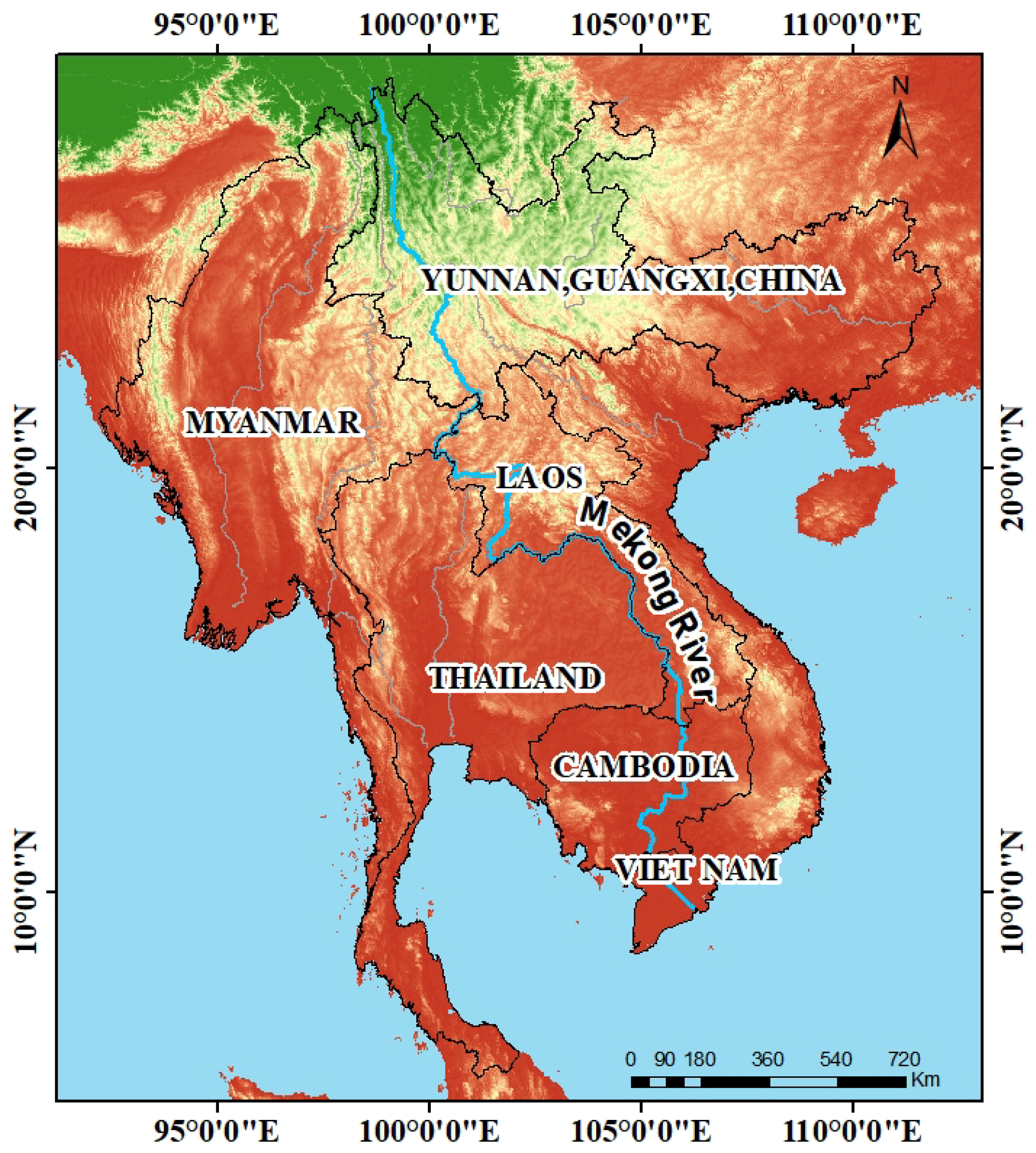
Figure 1. Distribution maps of Myanmar (MM), Laos (LA), Thailand (TH), Cambodia (KH), Vietnam (VN) and Guangxi and Yunnan provinces of China (CN) in the study area.
Remotesensing 14 05982 g001
Figure 2. Flow chart of enhanced vegetation index (EVI) trend extraction and spatial correlation analysis.
Remotesensing 14 05982 g002
Figure 3. Spatial distribution of land use/land cover (LULC) conversion.
Remotesensing 14 05982 g003
Figure 4. Significant trends in EVI of forests and grasslands without type change: (a) significant trends in EVI of forests; (b) significant trends in EVI of grasslands.
Remotesensing 14 05982 g004
Figure 5. Area and slope distributions of significant EVI trends for forests and grasslands with no change type change: (a) area of EVI trends for forests; (b) area of EVI trends for grasslands; (c) slope of EVI trends for forests; (d) slope of EVI trends for grasslands.
Remotesensing 14 05982 g005
Figure 6. Area and spatial distributions of polynomial trends for forests and grasslands with no change type change: (a,b) spatial distributions of polynomial trends for forests and grasslands; (c,d) area distributions of polynomial trends for forests.
Remotesensing 14 05982 g006
Figure 7. Trends in EVI for different forest management types: (a) area distribution of significant trends in EVI in forest management types; (b,c) proportion of upward and downward trends in EVI for forest management classes; (d,e) significant slope in EVI for forest management types.
Remotesensing 14 05982 g007
Figure 8. Spatial correlations in EVI with climate and environmental variables. (ap) Spatial clustering maps of EVI with bio01, bio04, bio05, bio06, bio08, bio09, bio10, bio12, bio15, elevation, topographic slope, surface net solar radiation (SSR), surface solar radiation downward (SSRD), soil temperature layer 1 (STl1), volumetric soil water layer 1 (SWVl) and total evaporation, respectively.
Remotesensing 14 05982 g008aRemotesensing 14 05982 g008b
Publisher’s Note: MDPI stays neutral with regard to jurisdictional claims in published maps and institutional affiliations.