Assessing Potential Spontaneous Combustion of Coal Gangue Dumps after Reclamation by Simulating Alfalfa Heat Stress Based on the Spectral Features of Chlorophyll Fluorescence Parameters

Abstract

The spontaneous combustion of coal gangue dumps after reclamation causes severe harm to the ecological environment surrounding mining areas. Using remote sensing technology to determine vegetation heat stress levels is an important way to evaluate the probability of a spontaneous combustion disaster. The canopy spectra and chlorophyll fluorescence (ChlF) parameters of alfalfa were collected through pot experiments to simulate different heat stress levels. Time series analyses of three ChlF (chlorophyll fluorescence) parameters showed that the regularity of the quantum efficiency of photosystem II (PSII) in light-adapted conditions (${\mathrm{Fv}}^{\prime }/{\mathrm{Fm}}^{\prime }$) was stronger during the monitoring period. The correlation coefficients between the three ChlF parameters and the canopy raw spectrum, first derivative spectrum, and vegetation indices were calculated, and the spectral features were found to be more correlated. Lasso regression was used to further screen spectral features, and the optimal spectral features were the raw spectral value at 741 nm (abbreviated as RS (741)) and NDVI (652, 671). To discriminate among heat stress levels accurately and automatically, we built a time convolution neural network. The classification results showed that when the sequence length is 3, the heat stress is divided into three categories, and the model obtains the highest accuracy. In combination with relevant research conclusions on the temperature distribution law of spontaneous combustion in coal gangue dumps, three heat stress levels can be used to assess the potential of spontaneous combustion in coal gangue dumps after reclamation. The research results provide an important theoretical basis and technical support for early warnings regarding spontaneous combustion disasters in reclaimed coal gangue dumps.

1. Introduction

Coal is one of the primary global energy sources [1]; coal production exceeded 8 billion tons in 2021. Although it provides energy security for the economy and society, coal mining also leads to great pressure on the ecological environment. The main by-product of coal mining is coal gangue, which is an important solid waste and one of the main sources of pollution in mining areas [2]. Under different mining methods and geological conditions, gangue accounts for about 10–15% of the total coal production [3]. Coal gangue is usually piled up, forming a coal gangue dump [4]. With long-term exposure to the natural environment, coal gangue will undergo weathering, oxidation, and other reactions. Organic matter and inorganic matter in waste rock oxidize and heat up, which could induce spontaneous combustion [5]. Further, the accumulation of coal gangue could provide favorable conditions for spontaneous combustion. When a spontaneous combustion disaster occurs, carbon monoxide, hydrogen sulfide, sulfur dioxide, and other gases are released, which leads to severe atmospheric pollution. In addition, it also causes heavy metal pollution in soil and groundwater [6,7].

With yearly increases in coal production, the number of coal gangue dumps is also increasing. According to statistics (which are still incomplete), there are nearly 10,000 coal gangue dumps in China, of which more than 1700 have experienced spontaneous combustion [8,9]. In light of this, in 2018, the Chinese government launched a three-year environmental protection plan. This plan has led to the treatment of coal gangue hills in major economic zones in China. However, field investigations have found that the reclaimed coal gangue dumps may still experience re-ignition [10]. This phenomenon is not only found in China but has also been reported all over the world in related research [11,12]. In addition to polluting the environment, the spontaneous combustion of reclaimed coal gangue dumps will also lead to surface soil cracking and large-scale vegetation damage [13,14], leading to severe ecosystem damage. The best way to avoid a spontaneous combustion disaster is prevention, the key to which is establishing an appropriate early warning method.

The surface temperature of exposed gangue dumps should be monitored using thermal infrared remote sensing to identify internal fire sources [15,16,17,18]. However, reclaimed gangue dumps often have covers of soil and vegetation; only when spontaneous combustion results in the destruction of surface vegetation can the thermal infrared sensor play a role. In recent years, reports that vegetation can be used as an early warning indicator of spontaneous combustion disasters in reclaimed coal gangue dumps have appeared [19,20]. Abramowicz et al. [20] found that changes in the health of vegetation in gangue mountain ecosystems could indicate increases in the ground temperature and can even help determine the direction of spontaneous combustion through vegetation, while discussing the possibility of identifying potential ignition points at the surface through vegetation. Sloss [21] identified the process of heat release rates with time for internal shade combustion and complete ignition spontaneous combustion of the potential ignition point of coal gangue mountains, concluding that the best time for fire prevention and control—irrespective of whether the fire source is shade combustion or final ignition—is the early heat release rate in the rising process, that is, the stage of heat accumulation. At this stage, the soil layer in the corresponding area is heated, and the surface vegetation experiences heat stress. Different intensities of fire sources will lead to different heat stress levels on surface vegetation; it is worth focusing on the use of this relationship to warn of spontaneous combustion disasters. The first problem to be solved is the accurate discrimination of the heat stress level.

Under different environmental stresses, vegetation’s physiological and biochemical parameters change significantly [22,23]. Remote sensing technology can monitor vegetation stresses quickly and accurately [24]. Spontaneous combustion of potential fire sources in coal gangue dumps is a form of typical environmental stress for surface vegetation. The selection of stress-sensitive physiological and biochemical parameters of vegetation can amplify the differences between different stress levels and facilitate the discrimination of stress levels using remote sensing.

Several studies have demonstrated that ChlF is an effective measure reflecting plant photosynthetic function [25], and is widely used in studies on functional changes in the photosynthetic structure of plants subjected to environmental stresses [26,27,28]. According to the different measurement methods for ChlF, it can be divided into laser-induced fluorescence and sunlight-induced fluorescence [29]. In this paper, laser-induced fluorescence is used, which is an important means to study the fluorescence remote sensing of terrestrial vegetation. $\mathrm{Fv}/\mathrm{F}\mathrm{m}$ and ${\mathrm{Fv}}^{\prime }/{\mathrm{Fm}}^{\prime }$ represent the quantum efficiency of photosystem II (PSII) in dark-and light-adapted conditions, respectively, and the healthy vegetation generally remains above 0.7 [30]. PhiPS2 is the actual photochemical efficiency of PS II, which decreases obviously when plants are stressed. qP and qN are the photochemical burst coefficient and non-photochemical burst coefficient, respectively, which represent the coefficients for plants to convert the total light energy into chemical energy and heat dissipation. From the point of view of applicability, this paper focuses on changes in the ChlF parameters of vegetation in heat stress and light-adapted conditions in coal gangue dumps.

The theoretical basis of ChlF indicates that it can adequately reflect the health status of vegetation experiencing stress. In recent years, many researchers have determined environmental stresses based on the spectral features of ChlF parameters. Alexander et al. [29] used steady-state fluorescence Fs to track changes in the photosynthesis processes of plants under water, temperature, and nitrogen stress through remote-sensing monitoring. The results show that water stress is related to decreases in the Fs signal intensity of red light and far-red light measured at the leaf and canopy level, and heat stress leads to an unstable decrease in Fs, exhibiting a downward trend. Gu et al. [31] extracted spectral features based on hyperspectral data and inverted several ChlF parameters of plants at different growth stages under waterlogging stress by constructing a back propagation neural network (BPNN) model. Their experimental results showed that the spectral features of ChlF parameters extracted were strongly correlated with plant waterlogging stress in different periods. Jia et al. [32] explored the quantitative relationship between spectral features such as the vegetation index, red edge position, and wavelet features and $\mathrm{Fv}/\mathrm{F}\mathrm{m}$ and ${\mathrm{Fv}}^{\prime }/{\mathrm{Fm}}^{\prime }$ through winter wheat nitrogen stress experiments. Their results showed that traditional vegetation indices and wavelet features could successfully detect $\mathrm{Fv}/\mathrm{F}\mathrm{m}$ and ${\mathrm{Fv}}^{\prime }/{\mathrm{Fm}}^{\prime }$ in various scenarios. Further, under high-temperature stress, the ChlF parameters are excellent indices reflecting the photosynthetic performance of vegetation [33,34,35]. Therefore, it is feasible to evaluate the vegetation stress using the spectral features of chlorophyll fluorescence [36].

From this perspective, the objectives of this study include: (1) ascertaining the spectral features most related to vegetation ChlF parameters under heat stress; (2) building a time convolutional network model with powerful generalization capability to discriminate the vegetation heat stress level based on multivariate spectral features; and (3) discussing, through relevant research on the distribution law of the spontaneous combustion temperature of coal gangue dumps, the applicability of discrimination results of the heat stress level for early warning systems regarding the spontaneous combustion of coal gangue dumps after reclamation.

2. Materials and Methods

2.1. Experimental Design

The heat stress simulation experiment was carried out in the canopy of Yangzhou University’s potted experiment site in Yangzhou City, Jiangsu Province (119°25′N, 32°23′E) in the autumn of 2020. Alfalfa, a common herbaceous plant used in coal gangue dump reclamation, was selected as the plant under study, and Algonquin was the tested alfalfa variant [37]. Sowing occurred on 10 September 2020, with a sowing density of 10 holes in each pot and two seeds in each hole. When the sample grew to three leaves, the seedlings were fixed as 10 plants in each pot and harvested on 15 November 2020. The diameter of the pelvic floor was about 20 cm, the largest diameter was about 28 cm, the height of the pelvic floor was about 31.5 cm, and the vacant weight was about 0.54 kg. Before sowing, 10 kg of air-dried loam after drying was filled in each pot, and 5.28 g of compound fertilizer (N-P-K ratio of 15%-15%-15%) was mixed. After sowing, about 1 kg of soil was evenly covered, and the relative water content of all treated soils was controlled to about 60%. The test site design is shown in Figure 1.

The first crop of alfalfa was sown for about 60 days to flowering. The heat stress gradient experiment commenced on 16 October 2020, one month before flowering. By 15 November 2020, data was collected eight times. A control group and five experimental groups were set: T1 = 60 °C, T2 = 90 °C, T3 = 120 °C, T4 = 150 °C, and T5 = 180 °C, where experiments were repeated five times each. The heat source was placed at a depth of 30 cm in the soil layer according to the thickness of the surface cover [38], which is usually the case in reclamation.

2.2. Data Acquisition

2.2.1. Measurement of ChlF Parameters

ChlF parameters were obtained using an LI-6800 photosynthetic-fluorescence measuring instrument (LiCOR Inc., Lincoln, NE, USA). LI-6800 comprises the main engine and an analyzer. The main engine is connected to the analyzer through a signal transmission line and a gas duct. The front end of the analyzer is a fluorescent leaf chamber, which can sandwich plant leaves with an area of few than 6 cm². Before measuring the fluorescence parameters, the alfalfa leaves were put into the fluorescence leaf chamber, and the main parameters were then set at the main engine: the gas flow rate was 500, the ambient temperature and air humidity were consistent with the humidity of the test site on the same day, the carbon dioxide concentration was set to 400, the induced light intensity was set according to the light intensity at the time of measurement, and the induced pulse light was multiphase. Fluorescence measurement began at about 11:00 a.m. on the monitoring day. Three pots were selected for each treatment, three plants were selected for each pot, and flag leaves were selected for measurement. In this experiment, ChlF parameters in light-adapted conditions were obtained; therefore, the dark-adapted process of leaves was not designed before each measurement. The main fluorescence parameters obtained include PhiPS2, ${\mathrm{Fv}}^{\prime }/{\mathrm{Fm}}^{\prime }$, and qP; their calculation equations are shown in (1)–(3).

$${Fv}^{\prime }/{Fm}^{\prime }=({Fm}^{\prime }-{Fo}^{\prime })/{Fm}^{\prime }$$

(1)

$$PhiPS2=({Fm}^{\prime }-Fs)/{Fm}^{\prime }$$

(2)

$$qP=1-(Fs-{Fo}^{\prime })/({Fm}^{\prime }-{Fo}^{\prime })$$

(3)

In the equations, fluorescence intensity values—including steady-state fluorescence (Fs), maximum fluorescence (Fm′) in light-adapted conditions, minimum fluorescence (Fo′) in light-adapted conditions, and variable fluorescence (Fv′) in light-adapted conditions—can be measured.

2.2.2. Measurement of Canopy Spectrum

The hyperspectral data was acquired using a portable ground object spectrometer SVC HR-1024i (Spectra Vista Corporation SVC HR-1024I). The alfalfa canopy reflectivity was measured in the range of 350–2500 nm, with sampling intervals of 1.5 nm (350–1000 nm), 3.8 nm (1000–1885 nm), and 2.5 nm (1885–2500 nm); the resampling interval was 1 nm. Because ChlF is mainly located in the visible wavelength region [39], only the 400–800 nm band is used in this paper.

The measurement was synchronized with the temperature gradient test, which was measured for the first time on 16 October 2020, and thereafter every four days. Sunny and windless weather was chosen, the canopy reflectivity data was measured from 10:00 to 14:00, and rainy days were disregarded. Up to 15 November 2020, spectral data were collected 8 times. A standard whiteboard was used for calibration during measurement. A hand-held optical fiber probe was used to measure alfalfa potted plants, and 3 pots were selected for the control group and each temperature treatment, and each pot was measured 6 times. The measured mean value for each group was taken as the true value for alfalfa canopy spectral reflectance. During the measurement, the standard whiteboard correction was carried out every 30 min.

2.3. Methods

2.3.1. Spectral Data Processing

 (1)

Raw spectrum

To suppress noise, all of the collected canopy original spectral data were smoothed. The smoothing algorithm adopted the Gaussian weighted moving average and used the spectral curves collected using Matlab 2017a (MathWorks, Natick, MA, USA) to calculate the average value, which helped reduce the intra-group differences. Then, the mean spectral curve was smoothed by one-dimensional Gaussian filtering along the spectral direction. The sliding window was set to 5.

 (2)

First derivative spectrum

The differential processing of the canopy spectrum can decrease the influence of background information on spectral data [40]. The first-derivative spectrum of spectral reflectance is calculated to highlight the target spectral features by Equation (4).

$$R^{\prime }({\lambda }_i)=[R({\lambda }_i+1)-R({\lambda }_i-1)]/2\mathsf{\Delta }\lambda$$

(4)

where ${\lambda }_i$ is the wavelength; $R({\lambda }_i)$ and $R^{\prime }({\lambda }_i)$ are the reflectance and first-derivative spectrum of the wavelength ${\lambda }_i$, respectively; and $\mathsf{\Delta }\lambda$ is the interval between the wavelength ${\lambda }_i-1$ and ${\lambda }_i$.

 (3)

Vegetation Index

The vegetation index was constructed using the two-band combination method of the raw canopy spectrum and compared with the conventional index (

Table 1. Vegetation indices related to ChlF parameters.

Index Type	Index Name (Abbreviation)	Equation 1
ChI VI	Transformed chlorophyll absorption in reflectance index (TCARI)	$3\times [(R_{710}-R_{680})-0.2\times (R_{700}-R_{560})(R_{710}/R_{680})]$ [42]
	Modified chlorophyll absorption ratio index (MCARI)	$(R_{700}-R_{670})-0.2\times (R_{700}-R_{550})(R_{700}/R_{670})$ [43]
	MERIS terrestrial chlorophyll index (MTCI)	$(R_{750}-R_{710})/(R_{750}-R_{680})$ [44]
	Modified MERIS terrestrial chlorophyll index (MMTCI)	$(R_{750}-R_{680}+0.03)(R_{750}-R_{710})/(R_{750}-R_{680})$ [45]
Pigment VI	Plant pigment ratio (PPR)	$(R_{550}-R_{450})/(R_{550}+R_{450})$ [46]
Structure VI	Structure insensitive pigment index (SIPI)	$(R_{800}-R_{445})/(R_{800}-R_{680})$ [47]
	Optimized soil-adjusted vegetation index (OSAVI)	$1.16\times (R_{800}-R_{670})/(R_{800}-R_{670}+0.16)$ [48]
	Green normalized difference vegetation index (GNDVI)	$(R_{750}-R_{550})/(R_{750}+R_{550})$ [49]

¹ $R_{\lambda }$ = reflectance at wavelength ${\lambda }_{}$.

). The two-band combination method included the ratio vegetation index ($RVI({\lambda }_1,{\lambda }_2)$), normalized difference vegetation index ($NDVI({\lambda }_1,{\lambda }_2)$), and difference vegetation index ($DVI({\lambda }_1,{\lambda }_2)$). The band combinations were available between 400 and 800 nm, and their equations [41] are as follows:

$$NDVI({\lambda }_1,{\lambda }_2)=(R_{{\lambda }_1}-R_{{\lambda }_2})/(R_{{\lambda }_1}+R_{{\lambda }_2})$$

(5)

$$RVI({\lambda }_1,{\lambda }_2)=R_{{\lambda }_1}/R_{{\lambda }_2}$$

(6)

$$DVI({\lambda }_1,{\lambda }_2)=R_{{\lambda }_1}-R_{{\lambda }_2}$$

(7)

where ${\lambda }_1$ and ${\lambda }_2$ are wavelengths (nm); $R_{{\lambda }_1}$ and $R_{{\lambda }_2}$ are the reflectances at wavelengths ${\lambda }_1$ and ${\lambda }_2$, respectively; and ${\lambda }_1\ne {\lambda }_2$.

2.3.2. Spectral Feature Extraction of ChlF Parameters

 (1)

Correlation Analysis

The spectral parameters (raw spectra, first-order derivative spectra, and vegetation indices) were correlated with the alfalfa ChlF parameters (PhiPS2, ${\mathrm{Fv}}^{\prime }/{\mathrm{Fm}}^{\prime }$, and qP) using Pearson correlation coefficients (Equation (8)). The highly correlated spectral features were selected in the appropriate band range.

$$r(X,Y)=\frac{Cov(X,Y)}{{\delta }_X{\delta }_Y}$$

(8)

where $Cov(X,Y)$ is the covariance of $X$ and $Y$, ${\delta }_X$ is the variance of $X$, and ${\delta }_Y$ is the variance of $Y$.

 (2)

Lasso Regression Analysis

The Lasso (least absolute shrinkage operator) regression model is an important regression model in the field of machine learning [50]. The method obtains a relatively stable model by constructing a penalty function. This allows the model to compress the coefficients of some independent variables. Through regularization, the regression coefficients of some independent variables are compressed to zero. At the same time, Lasso regression retains the advantage of subset shrinkage and is a biased estimation model dealing with multicollinearity data (Equation (9)).

$$\underset{{\beta }_0,\beta }{\min }(\frac{1}{2N}{\displaystyle \sum _{i=1}^N(y_j-\beta x_i^T-{\beta }_0)+\lambda {\displaystyle \sum _{j=1}^p\left|{\beta }_j\right|}})$$

(9)

where $N$ is is the sample number, $y_j$ is the predicted true value, $x_i$ is the observed value, ${\beta }_0$ is the bias, $\beta$ is the weight of the observed variable, and $\lambda$ is a non-negative regularization parameter. $\lambda {\displaystyle {\sum }_{j=1}^p\left|{\beta }_j\right|}$ is called $L^1$ regularization.

2.3.3. Discrimination of the Heat Stress Level Using TCN

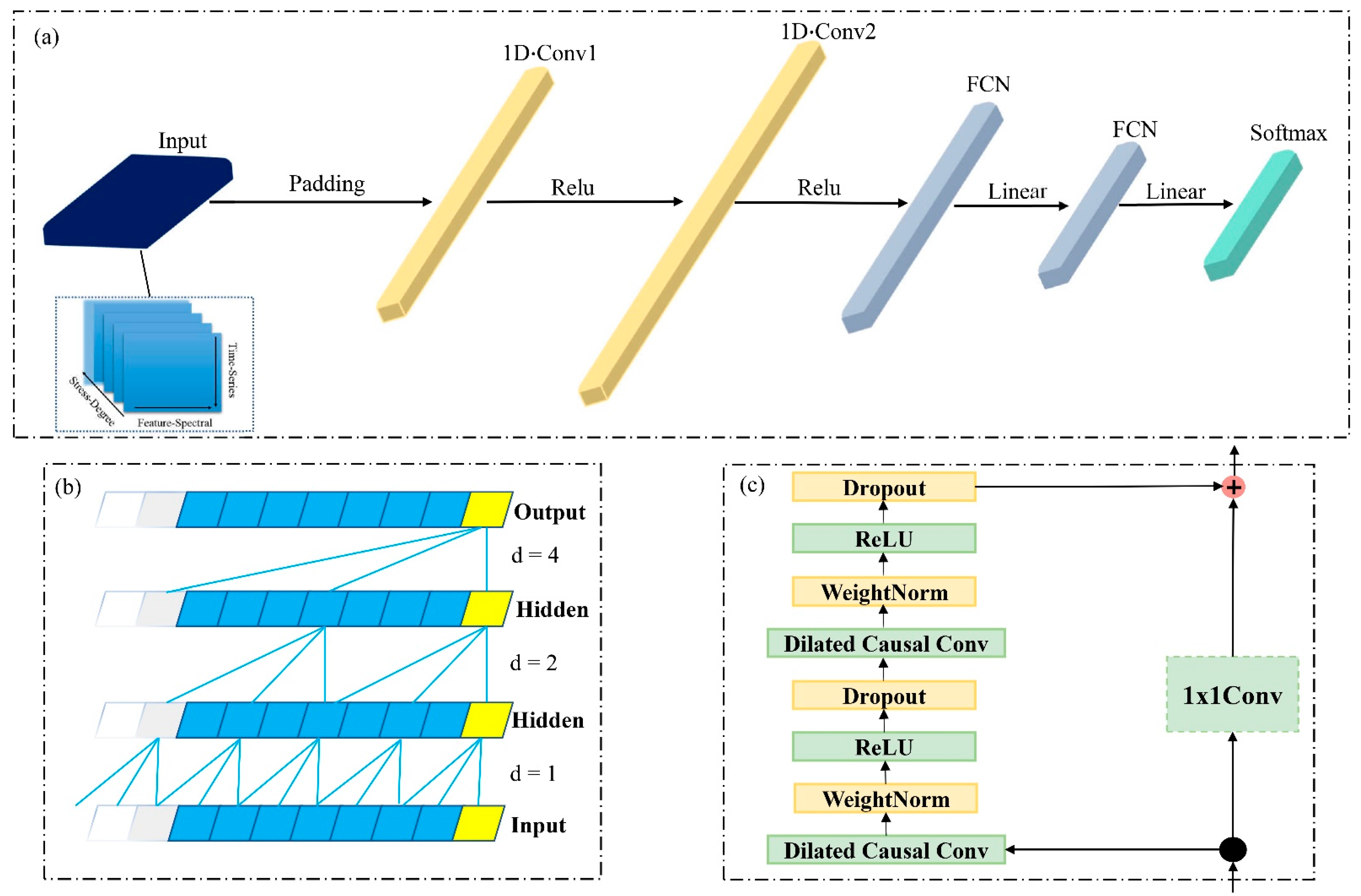
The modeling of time series data is the key to distinguishing the heat stress levels by using the spectral features of ChlF parameters of alfalfa. In recent years, rapid developments in deep learning have made important contributions to solving this problem. Among them, sequence modeling is primarily based on recurrent neural networks (RNNs), and their variants—LSTM, gated recurrent units (GRUs), back-propagation through time (BPTT), etc. However, studies have shown that convolution structures are superior to RNNs in series modeling tasks in recent years [51]. A time convolution network (TCN) originates from a convolution neural network, it performs better in time series prediction tasks than LSTM [52]. TCN has a stronger generalization ability, it can not only process one-dimensional time series data but can also process two-dimensional images. TCN k in this paper primarily comprises two one-dimensional convolution layers, two full connection layers, and a softmax classification layer. Similar to image data processing, a three-dimensional matrix of input data was constructed with dimensions of (1) specific features, (2) time series, and (3) stress levels, as illustrated in Figure 2a.

Because of the causality of convolution, the architecture of TCN ensures that time series data does not go missing. Convolution structures emphasize the use of 1D fully convolution network (FCN) architectures, set each hidden layer to maintain the same length as the input layer, and keep the length at zero (kernel size). It can be simply described as follows:

$$\mathrm{TCN}=1\mathrm{D}\mathrm{FCN}+\mathrm{causal}\mathrm{convolutions}$$

(10)

Simple causal convolution can only deal with linear time series data in a network. In some long-time series tasks, a linear review of the data alone is not sufficient. An exponential receptive field is achieved in the TCN structure by the dilated convolution method. That is, for a one-dimensional sequence input $\mathrm{x}\in {ℝ}^{\mathrm{n}}$ and a filter $f:\left\{0,\dots ,k-1\right\}\to ℝ$, the dilated convolution operation F on sequence element s is defined as

$$F\left(s\right)=\left(\mathrm{X}{\ast }_{d}f\right)\left(s\right)={\displaystyle \sum _{i=0}^{k-1}f\left(i\right)}\cdot {\mathrm{X}}_{s-d\cdot i·}$$

(11)

where d is the dilated factor; k denotes the filter size; and s-d·i is the past direction. It can be seen from the formula that the basic principle of expansion involves adding a filter with a specific step size between adjacent nodes. The stronger expansion enables the output to obtain a wider range of inputs at the upper layer, effectively expanding the receptive field of the convolution network, as illustrated in Figure 2b.

The application of residual links in the time convolution network has improved owing to the high-quality research on deep residual networks (Resnet) [53] conducted in 2016. The TCN residual block contains a branch that leads to a series of transformations $\mathcal{F}$, the output of which is added to the input X of the block:

$$\mathrm{o}=\mathrm{Activation}\left(\mathrm{X}+\mathcal{F}\left(\mathrm{X}\right)\right)$$

(12)

In the residual block, TCN has two layers of extended causal convolution and nonlinearity, for which we use a rectified linear unit (ReLU). Further, weight normalization is applied to the convolution filters. In addition, spatial attenuation is added after each dilated convolution for regularization, as illustrated in Figure 2c.

In this study, the main data source for discriminating heat stress levels is one-dimensional hyperspectral data. Considering practical applicability, the data sources in the large-scale monitoring of coal gangue hills are mostly UAV images or satellite remote sensing images; the advantages of TCN form the basis for its use in this study and subsequent work.

2.3.4. Evaluation Criteria

The sample data for constructing the model were divided into a training set (segmentation scale = 0.8) and test set (segmentation scale = 0.2). The coefficient of determination (R²) and root mean square error (RMSE) were used as indicators of its accuracy [54] (Equations (13) and (14)). Accuracy is defined as the degree of consistency between the model results and the true categories (Equation (15)). Ten-fold cross-validation was adopted for the training set [55].

$$R\mathrm{m}SE=\sqrt{\frac{{\displaystyle {\sum }_{i=1}^n{({\widehat{y}}_i-y_i)}^2}}{n}}$$

(13)

$$R^2=1-\frac{{\displaystyle {\sum }_{i=1}^n{({\widehat{y}}_i-y_i)}^2}}{{\displaystyle {\sum }_{i=1}^n{({\overline{y}}_i-y_i)}^2}}$$

(14)

$$Accuracy=\frac{n_{class}}{n}\times 100\%$$

(15)

where $y_i$ is the true value, ${\widehat{y}}_i$ is the predicted value, ${\overline{y}}_i$ is the mean value, $n$ is the number of samples, and $n_{class}$ is the number of correctly classified samples.

3. Results

3.1. ChIF Parameter Time Series Analysis

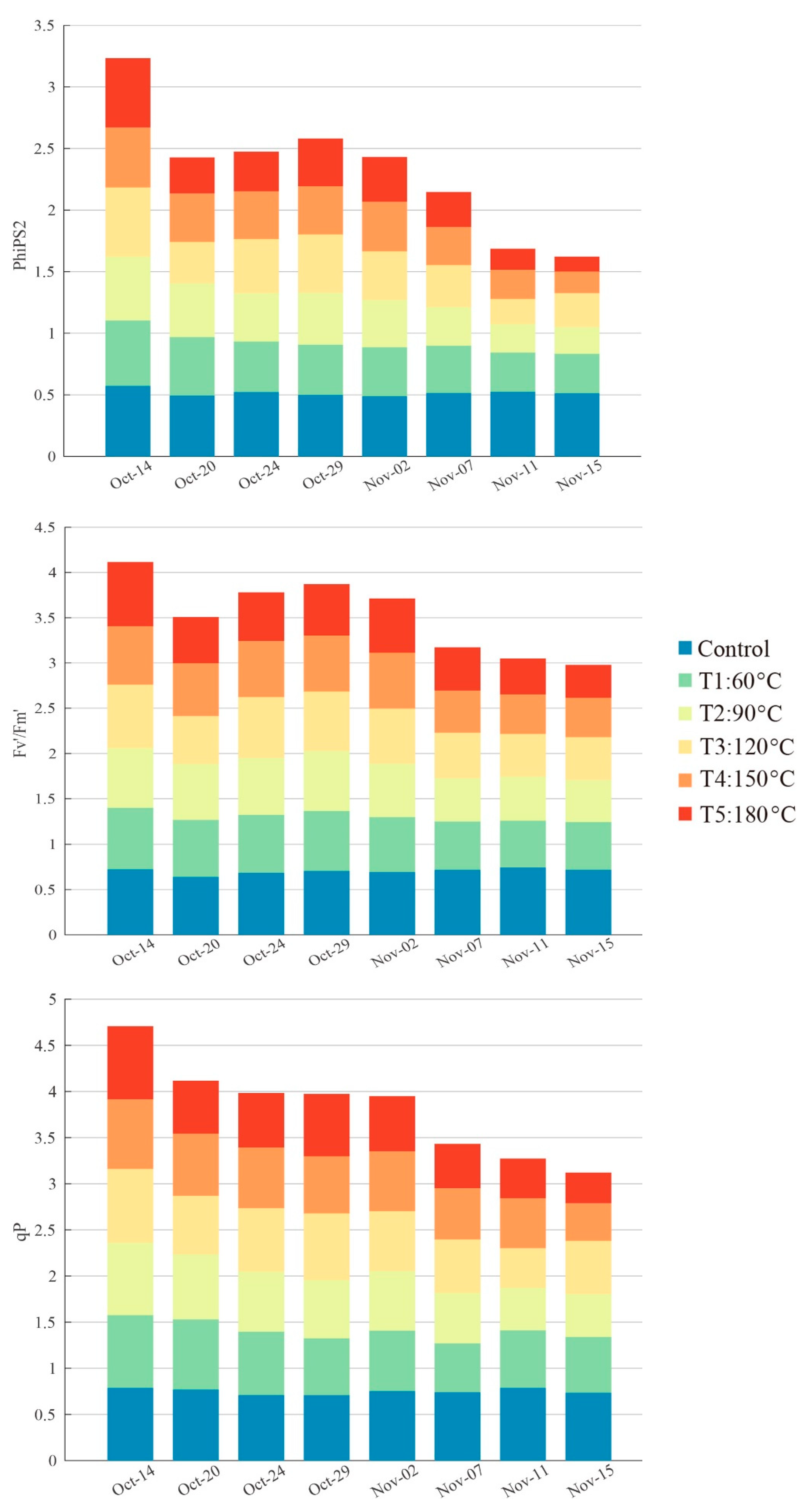
ChlF parameters are important indicators of the photosynthetic capacity of alfalfa. Under different heat stress levels, the ChlF parameters of alfalfa changed significantly. On 16 October 2020, the day after the first data collection, the soil layer was heated, and the ChlF parameters of alfalfa were measured eight times. Figure 3 shows the significant differences between the control group and the experimental groups at each measurement date, and the changes in the PhiPS2, ${\mathrm{Fv}}^{\prime }/{\mathrm{Fm}}^{\prime }$, and qP with time under different treatments. When the samples were collected on 16 October, the topsoil was not heated. At this time, the growth trend of alfalfa in the control group and the experimental group was similar, but there was no obvious difference in PhiPS2 and qP among the groups. After heating began, the significant differences between PhiPS2, and qP at each measurement date were weak in regularity. When focusing on the time series trend of fluorescence parameters in the overall monitoring period, the following can be observed: (1) PhiPS2: The control group exhibited little change during the entire monitoring period, while all treatments in the experimental group showed a downward trend. T3, T4, and T5 increased slightly after a rapid decline on 20 October. By 7 November, all experimental groups began to decline rapidly. Generally speaking, the PhiPS2 value in the control group was larger than that in the experimental group on each monitoring date, but it was difficult to find a consistent change rule in each treatment of the experimental group either on a single date or in the overall monitoring cycle; (2) ${\mathrm{Fv}}^{\prime }/{\mathrm{Fm}}^{\prime }$: As shown in Figure 3, the control group was larger than the experimental group on all dates, and the experimental group exhibited a downward trend. After 24 October, the size of each experimental group was consistent with the stress level. From 11 November, the experimental group dropped to a low point; T5 was lower than 0.4, and the vegetation was irreversibly damaged, which remained the same on 15 November. (3) qP: The change range of the control group was small during the monitoring period, while the experimental group still exhibited a decreasing trend. The changes in qP under different treatments were different on each date, which clearly had nothing to do with the stress level. After 7 November, T2, T4, and T5 decreased rapidly in the experimental group, but T1 and T3 did not change much.

According to the abovementioned analysis, ChlF is a suitable parameter to reflect the heat stress levels of alfalfa. The temporal change law is in accordance with the actual situation, and the photosynthetic capacity of plants is positively correlated with ${\mathrm{Fv}}^{\prime }/{\mathrm{Fm}}^{\prime }$, which is suitable for discriminating the heat stress levels of alfalfa [56].

3.2. Correlation Analysis of the Spectral Features and ChlF Parameters

3.2.1. Correlations among the Raw Spectrum, Derivative Spectrum, and ChlF Parameters

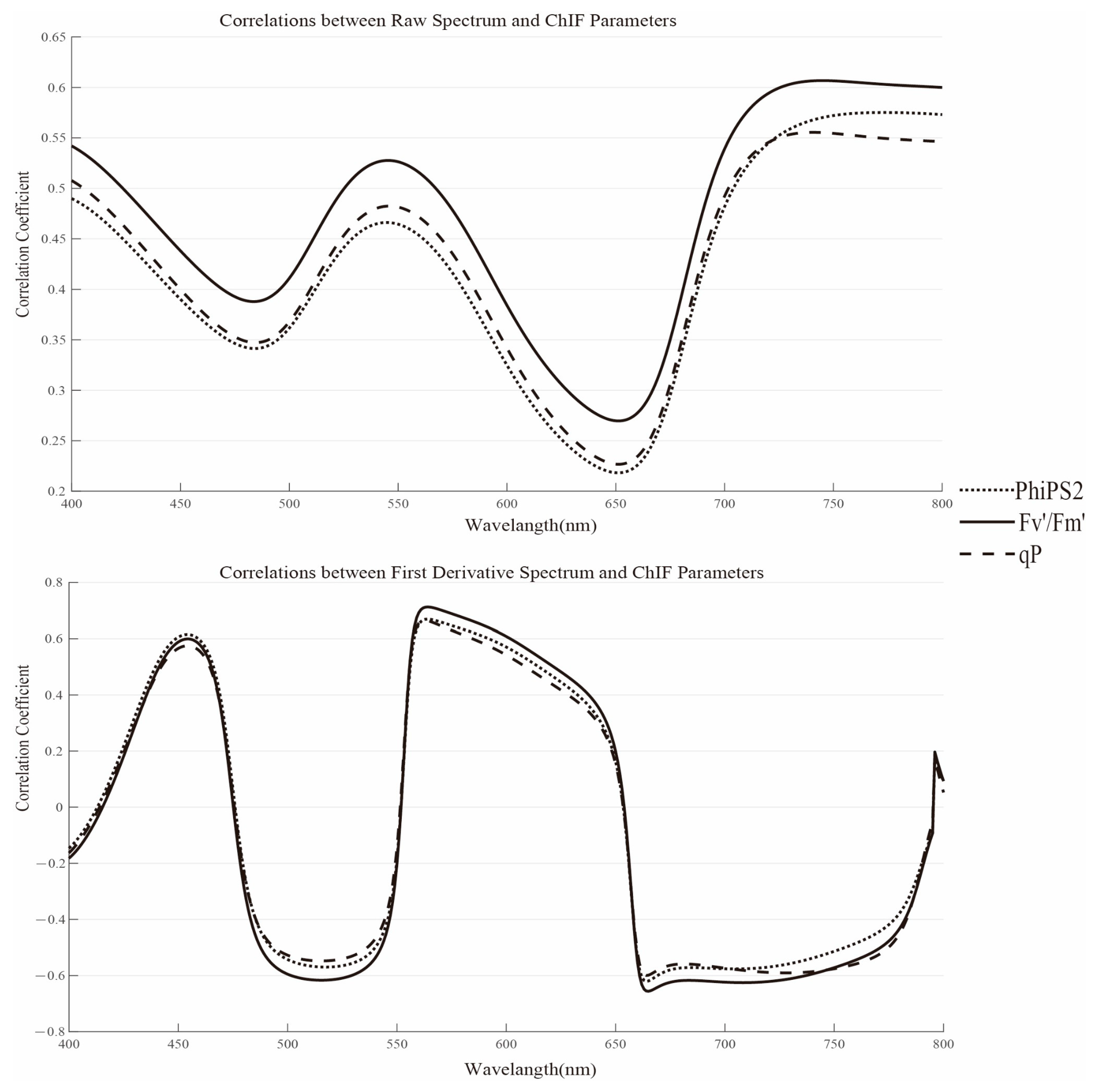
A correlation analysis of PhiPS2, ${\mathrm{Fv}}^{\prime }/{\mathrm{Fm}}^{\prime }$, and qP was performed using raw canopy spectrum and first-derivative spectrum data from the entire monitoring period (16 October–15 November; Figure 4). The results show that the change trends of the three parameters in the monitoring period are similar, the correlation between the raw spectrum and the first-order differential spectrum is uncertain, the correlation of ${\mathrm{Fv}}^{\prime }/{\mathrm{Fm}}^{\prime }$ is stronger than the other two parameters on the whole, and the maximum correlation coefficient also belongs to ${\mathrm{Fv}}^{\prime }/{\mathrm{Fm}}^{\prime }$. The maximum value of the raw spectrum and ${\mathrm{Fv}}^{\prime }/{\mathrm{Fm}}^{\prime }$ correlation appears at 741 nm (r = −0.61), and the maximum value of the first-order differential spectrum and ${\mathrm{Fv}}^{\prime }/{\mathrm{Fm}}^{\prime }$ correlation coefficient appears at 516 nm (r = −0.71). The spectral reflectance of the 400–800 nm band has no effect on water vapor absorption, and the first-order differential spectrum can suppress background noise to a certain extent; its correlation analysis with ChlF parameters is slightly better than that with the raw spectrum.

3.2.2. Correlation between Vegetation Indices and ChlF Parameters

In the hyperspectral remote-sensing monitoring of plant ChlF parameters, a large number of studies have shown that the relevant index located in visible light and red edge band can be used for the inversion of fluorescence parameters [57]. Therefore, we first calculated the correlation between the vegetation index of the canopy spectrum (Table 1) and PhiPS2, ${\mathrm{Fv}}^{\prime }/{\mathrm{Fm}}^{\prime }$, and qP. The results are shown in

Table 2. Coefficients of correlation (r) between existing spectral reflectance indices and the ChlF Parameters.

VI	r			VI	r
	PhiPS2	${\mathrm{Fv}}^{\prime }/{\mathrm{Fm}}^{\prime }$	qP		PhiPS2	${\mathrm{Fv}}^{\prime }/{\mathrm{Fm}}^{\prime }$	qP
SIPI	0.59	0.59 *	0.59 *	MCARI	0.51	0.56 *	0.52
OSAVI	0.51	0.52	0.50	PPR	0.42	0.49	0.46
GNDVI	0.31	0.36	0.29	MTCI	0.39	0.40	0.39
TCARI	0.53	0.67 *	0.55	MMTCI	0.62 *	0.64 *	0.59

* Indicates significant differences at the 95% confidence level.

. There are three absolute values of the correlation coefficient for the index calculation selected by the canopy spectrum greater than 0.6, including TCARI (r = 0.67) with ${\mathrm{Fv}}^{\prime }/{\mathrm{Fm}}^{\prime }$ and MMTCI (r = 0.62) and MMTCI (r = 0.64) with PhiPS2. The calculation results in Table 2 show that the correlation between these classical vegetation indices and fluorescence parameters is relatively weak. To determine better spectral features, it is necessary to construct vegetation indices with better correlations.

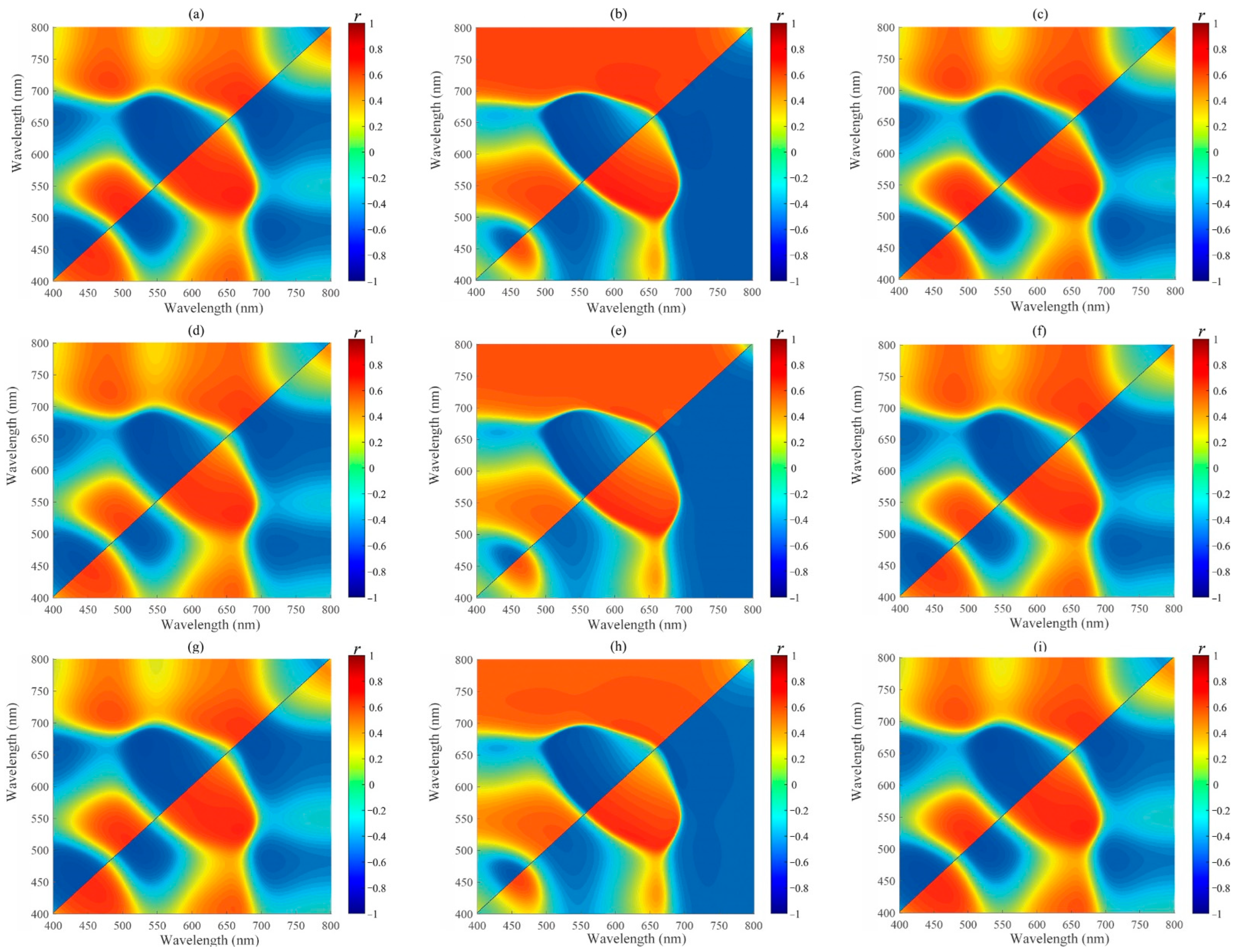
To find the best VI for estimating the ChlF parameters, the correlations between the ratio (RVI), the normalized difference (NDVI), and the difference (DVI) vegetation indices of the two bands in the 400–800 nm range with PhiPS2, ${\mathrm{Fv}}^{\prime }/{\mathrm{Fm}}^{\prime }$, and qP were systematically analyzed. Figure 5 shows a matrix of the correlation coefficients based on the different band combinations of the raw full-band spectrum and the ChIF parameters.

The results show that the main reason for the difference in the overall correlation between the spectral index and ChlF parameters is the construction mode of band combination, that is, the ratio and normalization are stronger than the difference, and the maximum correlation coefficient in each constructed index appears in the correlation analysis with ${\mathrm{Fv}}^{\prime }/{\mathrm{Fm}}^{\prime }$. The vegetation index was more strongly correlated with ${\mathrm{Fv}}^{\prime }/{\mathrm{Fm}}^{\prime }$ than PhiPS2 and qP. From Figure 5d–f, the three indices with the highest correlation coefficient r were selected, RVI (599, 611), DVI (570, 634), and NDVI (652, 671), with r being 0.71, 0.76, and 0.70, respectively. The three indices have a high correlation with ${\mathrm{Fv}}^{\prime }/{\mathrm{Fm}}^{\prime }$, which can be used as spectral features for ChlF parameter estimation.

3.3. Spectral Features of Lasso Regression Analysis

According to the previous analysis, ${\mathrm{Fv}}^{\prime }/{\mathrm{Fm}}^{\prime }$ values at the canopy scale are suitable to reflect the heat stress of alfalfa. After preliminary screening, five spectral features were obtained: RS (741), FDS (516), RVI (599, 611), DVI (570, 634), and NDVI (652, 671). The bands that constitute spectral characteristics are mainly concentrated in red-light and edge areas. Many spectral features obtained through correlation analysis may suffer from collinearity and other problems; therefore, it is necessary to further optimize spectral features. Lasso regression is used to reduce the dimensionality of feature parameters.

The Lasso regression model can reduce the dimensionality of multi-dimensional inputs. Figure 6 maps the training process and fitting results of selected canopy spectral features using Lasso regression. First, we need to determine the optimal regularization coefficient lambda (λ) and use 10-fold cross-validation for the dataset (n = 48). The training process of the Lasso regularity coefficient at the canopy scale is shown in Figure 6a. After many iterations, we obtain λ with the smallest RMSE as the optimal regularity coefficient of the model. The compressed spectral characteristic parameters are then obtained and the accuracy of the regression model is tested. The results are shown in

Table 3. Spectral features were selected by Lasso regression.

Lasso Regression Spectral Parameters	Regression Coefficients	R2_CV	RMSE_CV
RS (741)	2.80 × 10−3	0.67	9.10 × 10−3
FDS (516)	−4.94 × 10−2
RVI (599,611)	0
DVI (570,634)	0
NDVI (652,671)	1.82
Bias	2.12 × 10−2
Equation 1	$y=2.8\times {10}^{-3}{x}_1-4.94\times {10}^{-2}{x}_2+1.82x_3+2.12\times {10}^{-2}$

¹ y = $\mathrm{Fv}{}^{\prime }/\mathrm{Fm}{}^{\prime }$; $x_1$ = RS (741);$x_2$ = FDS (516);$x_3=$ NDVI (652,671).

and Figure 6b. Table 3 shows that the regression coefficients of RVI (599, 611) and DVI (570, 634) are both 0, which means that they are eliminated by the model. The R² and RMSE of the Lasso regression model with RS (741), FDS (516), and NDVI (652, 671) as independent variables were 0.67 and 9.10 × 10⁻³, respectively.

In the reflectance spectrum, the spectral information of ChlF is concentrated in the red-light and far red-light regions [58]. Although FDS (516) performs well in quantitative analyses, it has no physical significance and is not suitable for use as the spectral feature of ${\mathrm{Fv}}^{\prime }/{\mathrm{Fm}}^{\prime }$. Therefore, the optimal results for spectral characteristics are RS (741) and NDVI (652, 671).

3.4. Discrimination of the Heat-Stress Level

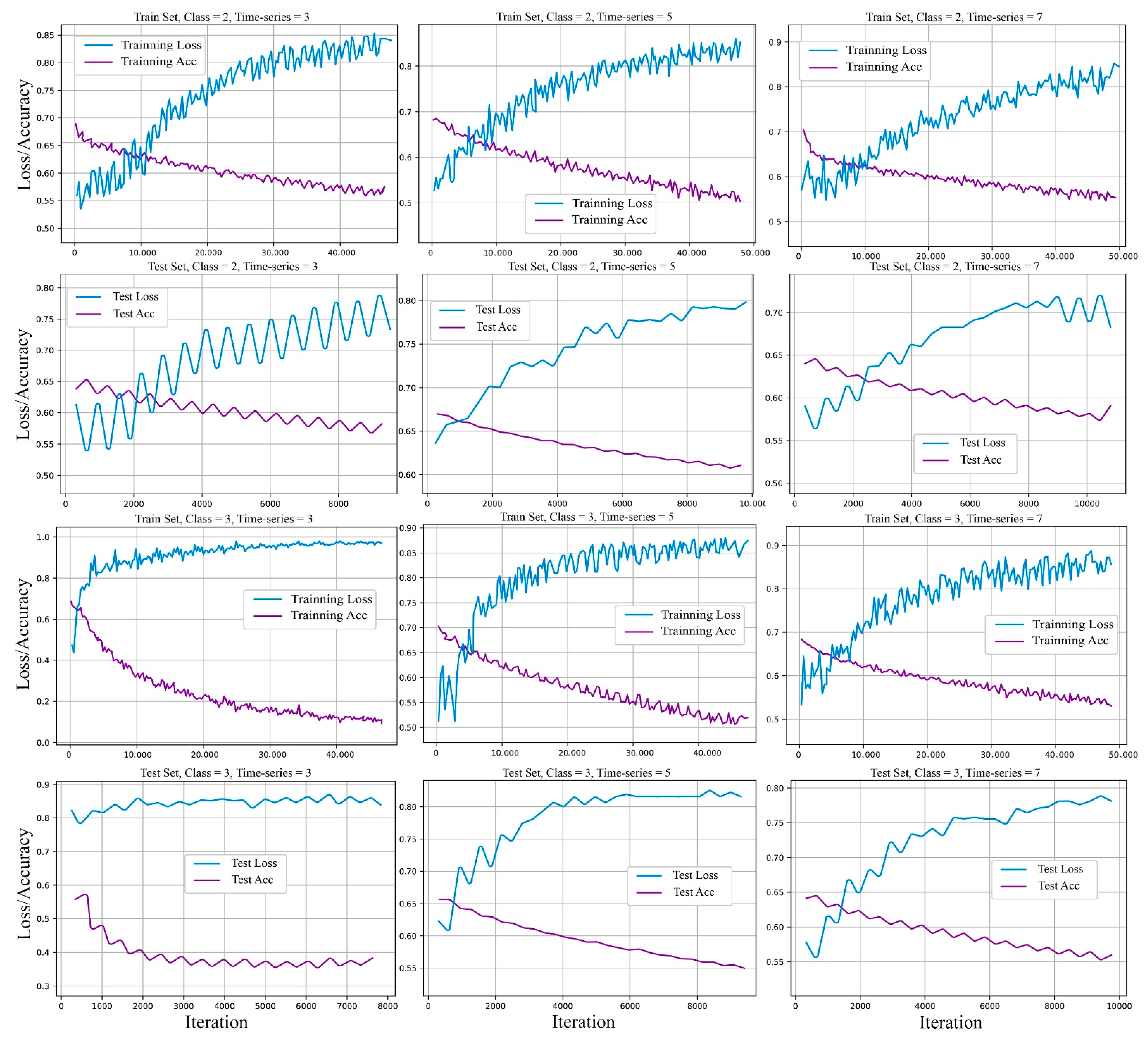
Using the spectral features of ChlF parameters to accurately discriminate the stress levels of plants should fully consider the time-series changes of spectral data, and while single-period estimation is sometimes feasible, these methods are often not well generalized. To solve this problem, this study uses the spectral features of time series as inputs to construct an SF-TCN model, which transforms the discrimination of plant stress levels into a classification problem; Figure 4 shows the network structure. To find the optimal model, the input layer data is set with uniform spectral features and different time series lengths, and different classification strategies are used to carry out experiments: (1) ${\mathrm{Fv}}^{\prime }/{\mathrm{Fm}}^{\prime }$ spectral features are used as input: RS (741) and NDVI (652, 671); (2) time series: the time series length is divided into 3, 5, and 7 (each time series length is a continuous date and does not repeat in reverse); (3) classification strategies: two categories (control group and experimental groups), three categories (control group; T1 and T2; and T3, T4, and T5), and six categories (control group and each of the five experimental groups). The number of samples in each test was determined by the length of the time series, and the ratio of the training set to the verification set was 4:1. The number of output layer categories was consistent with the number of stress level categories. The initial learning rate was 0.001, and the batch size was adjusted according to the sample size. The adaptive moment estimate (Adam) was selected by the network optimizer and the cross-entropy error function was adopted as the loss function. The model training and test results are shown in Figure 7. The model training accuracy under the six strategies in the figure is too low, and loss is difficult to converge, so it is not drawn.

As shown in Figure 7, the classification determines the overall accuracy of the model. The loss and accuracy of the training set and verification set of the two-class strategy are lower than those of the three-class strategy. When the heat stress level is divided into three categories, the accuracy of the model is obviously improved. When the time series length is 3, the convergence of model training set loss and accuracy is better, the accuracy of the test set is relatively highest, and the highest accuracy of the test set accuracy is about 87%. With increases in the length of the time series, the accuracy of the model decreases, and the effect is the worst when the time series length is 7. Overall, the SF-TCN model based on spectral features is suitable for discriminating the heat stress levels of alfalfa when the classification strategy is 3 and the time series length is 3.

4. Discussion

In this study, a conduct gradient test was conducted by simulating alfalfa heat stress in a coal gangue dump after reclamation. ChlF parameters and canopy spectra on alfalfa were collected. The stress level in alfalfa under heat stress was estimated by the SF-TCN model. The spectral features of ChlF parameters and the discrimination model of heat stress are crucial for the assessment of spontaneous combustion disasters of coal gangue after reclamation, which requires further discussion.

4.1. ${Fv}^{\prime }/{Fm}^{\prime }$ as an Indicator to Respond to Heat Stress t

High temperatures may cause irreversible damage to the photosynthetic system of plants [59], including PSII inactivation, PSII electron transport rate decreases, and thylakoid disintegration [33,60]. The high soil temperature caused by fire sources inside gangue dumps is more harmful to surface plants than high air temperatures [61]. Studies have proved that ChlF can quickly capture the instantaneous changes in plant physiological states and their responses to various environmental stresses [32,62]. Practically, when detecting plant responses to stress, dark-adapted conditions are usually impossible to achieve; therefore, the three ChlF parameters selected in this paper are all in light-adapted conditions. The results of the time-series analysis show that the value of ${\mathrm{Fv}}^{\prime }/{\mathrm{Fm}}^{\prime }$ for the higher temperature treatment exhibited a decreasing trend, followed by increases and then decreases, characterizing the physiological process from the stress response to irreversible damage in vegetation under heat stress, which is consistent with the actual situation; however, the rest of the parameters performed poorly. ${\mathrm{Fv}}^{\prime }/{\mathrm{Fm}}^{\prime }$ is a suitable parameter to respond to heat stress, and it is an excellent indicator for evaluating plant stress, nutrient status, and health status [29], which is consistent with previous studies [63].

4.2. Spectral Feature Selection and Heat Stress Level Discrimination Model

This study focuses on the spectral features of ChlF parameters that can reflect vegetation heat stress. The spectral features used to monitor ChlF parameters are reflectance information characterizing the fluorescence intensity, rather than definite physical quantities [64]. Furthermore, ChlF signals belong to weak information in the reflection spectrum [65], which must be enhanced and screened using mathematical methods. Through correlation analyses, we preliminary obtained the spectral features of ChlF parameters, and further determined that ${\mathrm{Fv}}^{\prime }/{\mathrm{Fm}}^{\prime }$ is a suitable parameter to respond to the heat stress of alfalfa. Multivariate variables may also exhibit collinearity. Lasso regression can reduce the dimensionality of data, and further optimize the three spectral features: RS (741), FDS (516), and NDVI (652, 671) through the results of regression analysis. The chlorophyll fluid emission spectrum ranges from around 650 nm to 850 nm and includes two broad band peaks centered in the red (685 nm) and far-red (740 nm) wavelength range [66]. Although FDS (516) is highly correlated with ${\mathrm{Fv}}^{\prime }/{\mathrm{Fm}}^{\prime }$, it cannot be used as an indicator. RS (741) and NDVI (652, 671) are in the sensitive spectral range of ChlF, which are ideal spectral features.

4.3. Potential for Early Warning of Spontaneous Combustion Disasters in Coal Gangue Dumps Using Heat Stress Levels

The discrimination of heat stress levels is crucial for evaluating the spontaneous combustion disasters of reclaimed coal gangue dumps. We constructed an SF-TCN model to classify the heat stress levels. The model classification results show that the accuracy is the highest when the stress level is divided into three categories (control group; T1 and T2; and T3, T4, and T5). The results are highly consistent with those of previous studies. Ref. [67] found that, in the heat accumulation stage, the best early warning time for spontaneous combustion of coal gangue dump is when the temperature on the critical surface (30 cm for the soil layer in this study) is about 60–80 °C, and the state of the internal heat source is relatively stable at this time, which is the best time for fire extinguishing. With the passage of time, the temperature gradually increases, and the heat source point may move inside, causing an area fire. When the temperature reaches 200 °C and above, the possibility of an above-ground fire increases sharply and is the time of highest fire danger.

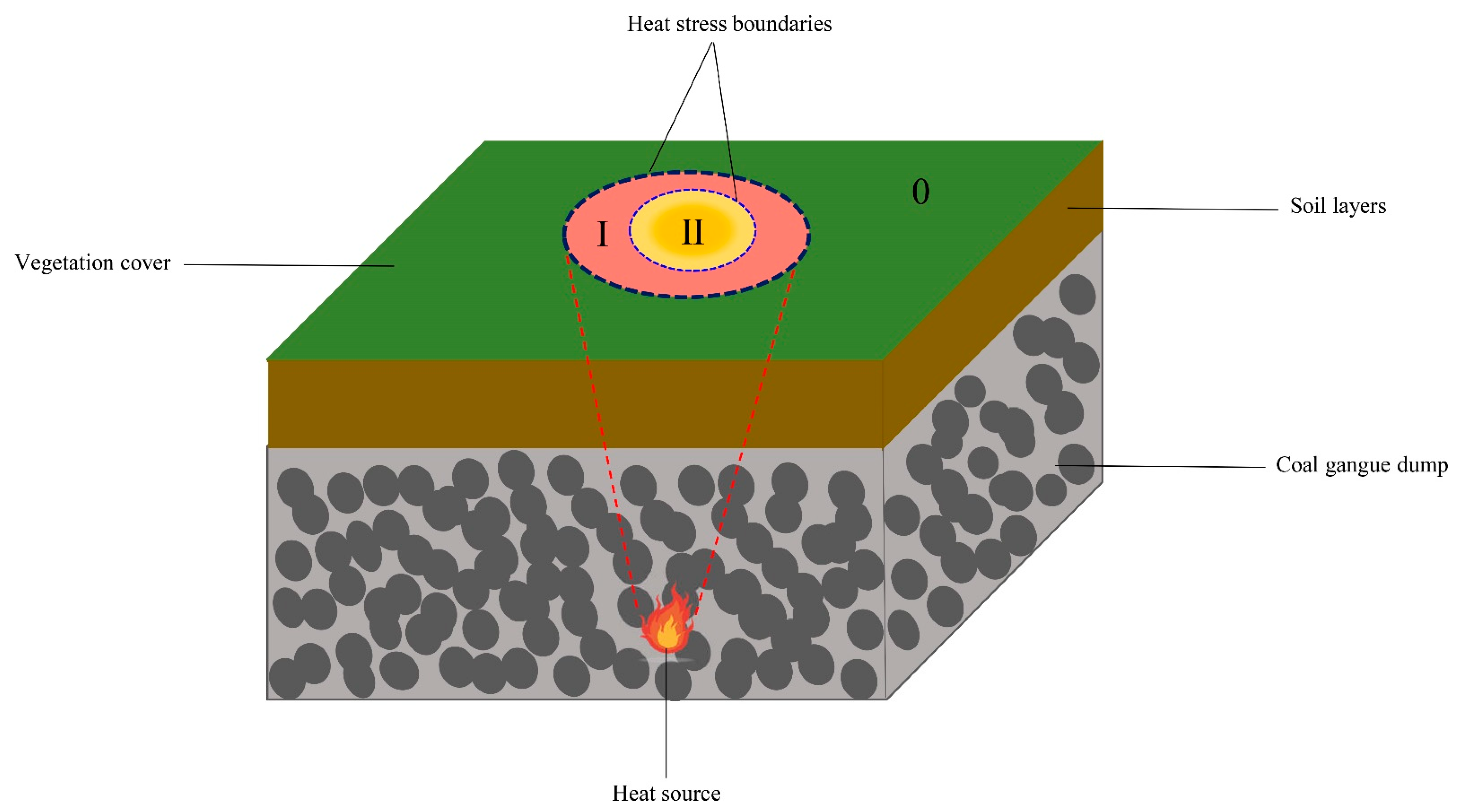
Based on the discrimination results of the heat stress level in this study and previous research conclusions, the early warning of spontaneous combustion can be divided into three grades according to the fire danger degree: the control group is O grade; 60 °C and 90 °C are I grade; and 120 °C, 150 °C, and 180 °C are II grade, as shown in Figure 8. During field applications, remote sensing data acquisition is mainly based on the canopy scale. The classification accuracy of the SF-TCN model constructed using multi-dimensional spectral features is high, and CNN as the core structure makes the model have strong generalization ability, which can be extended to the processing of unmanned aerial vehicle or satellite remote sensing images, giving it the strong potential to assess spontaneous combustion disasters of reclaimed coal gangue dumps. In the future, through remote sensing images, the heat stress level discrimination model can be used to draw a schematic, as shown in Figure 8, and divide the early warning levels of the spontaneous combustion of reclaimed coal gangue dumps.

5. Conclusions

Early warning of spontaneous combustion of gangue dumps is of great significance for ecological safety in mining areas. This study focuses on using the spectral features of ChlF parameters to discriminate the heat stress level of surface vegetation of reclaimed coal gangue dumps, and then contribute to the early warnings of spontaneous combustion disasters in reclaimed coal gangue dumps. The results showed that ${\mathrm{Fv}}^{\prime }/{\mathrm{Fm}}^{\prime }$ was more sensitive to heat stress than other parameters. RS (741) and NDVI (652, 671) were used as inputs to successfully construct an SF-TCN model with three heat stress levels. The consistency between the discrimination results of the heat stress level and previous research conclusions was discussed. The SF-TCN model has potential applicability in the early warning of spontaneous combustion disasters in reclaimed coal gangue dumps. Therefore, the focus of future research will be to use UAV remote sensing images or high-resolution satellite images for field monitoring. Further, this study also provides a new perspective on the remote-sensing monitoring of environmental stress such as drought stress and high-temperature stress.

References

1. Ren, H.; Zhao, Y.; Xiao, W.; Zhang, J.; Chen, C.; Ding, B.; Yang, X. Vegetation growth status as an early warning indicator for the spontaneous combustion disaster of coal waste dump after reclamation: An unmanned aerial vehicle remote sensing approach. J. Environ. Manag. 2022, 317, 115502. [Google Scholar] [CrossRef]
2. Xiao, W.; Chen, W.; Deng, X. Coupling and coordination of coal mining intensity and social-ecological resilience in China. Ecol. Indic. 2021, 131, 108167. [Google Scholar] [CrossRef]
3. Abramowicz, A.; Rahmonov, O.; Chybiorz, R. Environmental management and landscape transformation on self-heating coal-waste dumps in the Upper Silesian Coal Basin. Land 2020, 10, 23. [Google Scholar] [CrossRef]
4. Wang, Q.; Zhao, Y.; Yang, F.; Liu, T.; Xiao, W.; Sun, H. Simulating Heat Stress of Coal Gangue Spontaneous Combustion on Vegetation Using Alfalfa Leaf Water Content Spectral Features as Indicators. Remote Sens. 2021, 13, 2634. [Google Scholar] [CrossRef]
5. Querol, X.; Zhuang, X.; Font, O.; Izquierdo, M.; Alastuey, A.; Castro, I.; Van Drooge, B.L.; Moreno, T.; Grimalt, J.O.; Elvira, J. Influence of soil cover on reducing the environmental impact of spontaneous coal combustion in coal waste gobs: A review and new experimental data. Int. J. Coal Geol. 2011, 85, 2–22. [Google Scholar] [CrossRef]
6. Xiao, W.; Ren, H.; Sui, T.; Zhang, H.; Zhao, Y.; Hu, Z. A drone-and field-based investigation of the land degradation and soil erosion at an opencast coal mine dump after 5 years’ evolution of natural processes. Int. J. Coal Sci. Technol. 2022, 9, 1–17. [Google Scholar] [CrossRef]
7. Sun, Y.Z.; Fan, J.S.; Qin, P.; Niu, H.Y. Pollution extents of organic substances from a coal gangue dump of Jiulong Coal Mine, China. Environ. Geochem. Health 2009, 31, 81–89. [Google Scholar] [CrossRef]
8. Haibin, L.; Zhenling, L. Recycling utilization patterns of coal mining waste in China. Resour. Conserv. Recycl. 2010, 54, 1331–1340. [Google Scholar] [CrossRef]
9. Bian, Z.; Dong, J.; Lei, S.; Leng, H.; Mu, S.; Wang, H. The impact of disposal and treatment of coal mining wastes on environment and farmland. Environ. Geol. 2009, 58, 625–634. [Google Scholar] [CrossRef]
10. Ren, H.; Zhao, Y.; Xiao, W.; Yang, X.; Ding, B.; Chen, C. Monitoring potential spontaneous combustion in a coal waste dump after reclamation through UAV RGB imagery-based on alfalfa aboveground biomass (AGB). Land Degrad. Dev. 2022, 33, 2728–2742. [Google Scholar] [CrossRef]
11. Nádudvari, D.; Abramowicz, A.; Fabiańska, M.; Misz-Kennan, M.; Ciesielczuk, J. Classification of fires in coal waste dumps based on Landsat, Aster thermal bands and thermal camera in Polish and Ukrainian mining regions. Int. J. Coal Sci. Technol. 2021, 8, 441–456. [Google Scholar] [CrossRef]
12. Smoliński, A.; Dombek, V.; Pertile, E.; Drobek, L.; Magdziarczyk, M. An analysis of self-ignition of mine waste dumps in terms of environmental protection in industrial areas in Poland. Sci. Rep. 2021, 1, 8851. [Google Scholar] [CrossRef]
13. He, F.; Lan, Y.; Yan, H.; Duan, Q.; Yang, H. Research on key support technology based on green mining system and its application. In Proceedings of the 2011 International Conference on Remote Sensing, Environment and Transportation Engineering, Nanjing, China, 24–26 June 2011. [Google Scholar]
14. Abramowicz, A.K.; Rahmonov, O.; Fabiańska, M.J.; Nádudvari, Á.; Chybiorz, R.; Michalak, M. Changes in soil chemical composition caused by self-heating of a coal-waste dump. Land Degrad. Dev. 2021, 32, 4340–4349. [Google Scholar] [CrossRef]
15. Ren, H.; Zhao, Y.; Xiao, W.; Hu, Z. A review of UAV monitoring in mining areas: Current status and future perspectives. Int. J. Coal Sci. Technol. 2019, 6, 320–333. [Google Scholar] [CrossRef] [Green Version]
16. Hu, Z.; Xia, Q. An integrated methodology for monitoring spontaneous combustion of coal waste dumps based on surface temperature detection. Appl. Therm. Eng. 2017, 122, 27–38. [Google Scholar] [CrossRef]
17. Jendruś, R. Environmental Protection in Industrial Areas and Applying Thermal Analysis to Coal Dumps. Pol. J. Environ. Stud. 2017, 26, 137–146. [Google Scholar] [CrossRef]
18. Lewińska, P.; Dyczko, A. Thermal digital terrain model of a coal spoil tip–a way of improving monitoring and early diagnostics of potential spontaneous combustion areas. J. Ecol. Eng. 2016, 17, 170–179. [Google Scholar] [CrossRef]
19. Nádudvari, Á.; Abramowicz, A.; Ciesielczuk, J.; Cabała, J.; Misz-Kennan, M.; Fabiańska, M. Self-Heating Coal Waste Fire Monitoring and Related Environmental Problems: Case Studies from Poland and Ukraine. J. Environ. Geogr. 2021, 14, 26–38. [Google Scholar] [CrossRef]
20. Abramowicz, A.; Rahmonov, O.; Chybiorz, R.; Ciesielczuk, J. Vegetation as an indicator of underground smoldering fire on coal-waste dumps. Fire Saf. J. 2021, 121, 103287. [Google Scholar] [CrossRef]
21. Sloss, L.L. Assessing and Managing Spontaneous Combustion of Coal; IEA Clean Coal Centre: London, UK, 2015. [Google Scholar]
22. Singh, A.K.; Dhanapal, S.; Yadav, B.S. The dynamic responses of plant physiology and metabolism during environmental stress progression. Mol. Biol. Rep. 2020, 47, 1459–1470. [Google Scholar] [CrossRef]
23. Safdar, H.; Amin, A.; Shafiq, Y.; Ali, A.; Yasin, R.; Shoukat, A.; Hussan, M.U.; Sarwar, M.I. A review: Impact of salinity on plant growth. Nat. Sci. 2019, 17, 34–40. [Google Scholar]
24. Gerhards, M.; Schlerf, M.; Mallick, K.; Udelhoven, T. Challenges and future perspectives of multi-/Hyperspectral thermal infrared remote sensing for crop water-stress detection: A review. Remote Sens. 2019, 11, 1240. [Google Scholar] [CrossRef] [Green Version]
25. Joiner, J.; Yoshida, Y.; Vasilkov, A.P.; Middleton, E.M. First observations of global and seasonal terrestrial chlorophyll fluorescence from space. Biogeosciences 2011, 8, 637–651. [Google Scholar] [CrossRef] [Green Version]
26. Zarco-Tejada, P.J.; González-Dugo, V.; Berni, J.A. Fluorescence, temperature and narrow-band indices acquired from a UAV platform for water stress detection using a micro-hyperspectral imager and a thermal camera. Remote Sens. Environ. 2012, 117, 322–337. [Google Scholar] [CrossRef]
27. Panigada, C.; Rossini, M.; Meroni, M.; Cilia, C.; Busetto, L.; Amaducci, S.; Boschetti, M.; Cogliati, S.; Picchi, V.; Pinto, F. Fluorescence, PRI and canopy temperature for water stress detection in cereal crops. Int. J. Appl. Earth Obs. 2014, 30, 167–178. [Google Scholar] [CrossRef]
28. Meroni, M.; Rossini, M.; Picchi, V.; Panigada, C.; Cogliati, S.; Nali, C.; Colombo, R. Assessing steady-state fluorescence and PRI from hyperspectral proximal sensing as early indicators of plant stress: The case of ozone exposure. Sensors 2008, 8, 1740–1754. [Google Scholar] [CrossRef] [Green Version]
29. Ač, A.; Malenovský, Z.; Olejníčková, J.; Gallé, A.; Rascher, U.; Mohammed, G. Meta-analysis assessing potential of steady-state chlorophyll fluorescence for remote sensing detection of plant water, temperature and nitrogen stress. Remote Sens. Environ. 2015, 168, 420–436. [Google Scholar] [CrossRef] [Green Version]
30. Sharma, D.K.; Andersen, S.B.; Ottosen, C.O.; Rosenqvist, E. Wheat cultivars selected for high Fv/Fm under heat stress maintain high photosynthesis, total chlorophyll, stomatal conductance, transpiration and dry matter. Physiol. Plantarum. 2015, 153, 284–298. [Google Scholar] [CrossRef]
31. Gu, X.; Xu, P.; Qiu, H.; Feng, H. Monitoring the chlorophyll fluorescence parameters in rice under flooding and waterlogging stress based on remote sensing. In Proceedings of the 2014 World Automation Congress (WAC), Waikoloa, HI, USA, 3–7 August 2014. [Google Scholar]
32. Jia, M.; Li, D.; Colombo, R.; Wang, Y.; Wang, X.; Cheng, T.; Zhu, Y.; Yao, X.; Xu, C.; Ouer, G. Quantifying chlorophyll fluorescence parameters from hyperspectral reflectance at the leaf scale under various nitrogen treatment regimes in winter wheat. Remote Sens. 2019, 11, 2838. [Google Scholar] [CrossRef] [Green Version]
33. Janka, E.; Körner, O.; Rosenqvist, E.; Ottosen, C. High temperature stress monitoring and detection using chlorophyll a fluorescence and infrared thermography in chrysanthemum (Dendranthema grandiflora). Plant Physiol. Biochem. 2013, 67, 87–94. [Google Scholar] [CrossRef]
34. Gorbe, E.; Calatayud, A. Applications of chlorophyll fluorescence imaging technique in horticultural research: A review. Sci. Hortic. 2012, 138, 24–35. [Google Scholar] [CrossRef]
35. Zhou, R.; Yu, X.; Kjær, K.H.; Rosenqvist, E.; Ottosen, C.; Wu, Z. Screening and validation of tomato genotypes under heat stress using Fv/Fm to reveal the physiological mechanism of heat tolerance. Environ. Exp. Bot. 2015, 118, 1–11. [Google Scholar] [CrossRef]
36. Maimaitiyiming, M.; Ghulam, A.; Bozzolo, A.; Wilkins, J.L.; Kwasniewski, M.T. Early Detection of Plant Physiological Responses to Different Levels of Water Stress Using Reflectance Spectroscopy. Remote Sens. 2017, 9, 745. [Google Scholar] [CrossRef] [Green Version]
37. Xiong, X.; Liu, N.; Wei, Y.; Bi, Y.; Luo, J.; Xu, R.; Zhou, J.; Zhang, Y. Effects of non-uniform root zone salinity on growth, ion regulation, and antioxidant defense system in two alfalfa cultivars. Plant Physiol. Biochem. 2018, 132, 434–444. [Google Scholar] [CrossRef] [PubMed]
38. Wang, J.; Li, X.; Bai, Z.; Huang, L. The effects of coal gangue and fly ash on the hydraulic properties and water content distribution in reconstructed soil profiles of coal-mined land with a high groundwater table. Hydrol. Process. 2017, 31, 687–697. [Google Scholar] [CrossRef]
39. Zhao, F.; Li, R.; Verhoef, W.; Cogliati, S.; Liu, X.; Huang, Y.; Guo, Y.; Huang, J. Reconstruction of the full spectrum of solar-induced chlorophyll fluorescence: Intercomparison study for a novel method. Remote Sens. Environ. 2018, 219, 233–246. [Google Scholar] [CrossRef]
40. Thorp, K.R.; Wang, G.; Bronson, K.F.; Badaruddin, M.; Mon, J. Hyperspectral data mining to identify relevant canopy spectral features for estimating durum wheat growth, nitrogen status, and grain yield. Comput. Electron. Agr. 2017, 136, 1–12. [Google Scholar] [CrossRef] [Green Version]
41. Atzberger, C.; Darvishzadeh, R.; Immitzer, M.; Schlerf, M.; Skidmore, A.; Le Maire, G. Comparative analysis of different retrieval methods for mapping grassland leaf area index using airborne imaging spectroscopy. Int. J. Appl. Earth Obs. 2015, 43, 19–31. [Google Scholar] [CrossRef] [Green Version]
42. Zhang, L.; Zhang, H.; Niu, Y.; Han, W. Mapping maize water stress based on UAV multispectral remote sensing. Remote Sens. 2019, 11, 605. [Google Scholar] [CrossRef] [Green Version]
43. Zhang, C.; Kovacs, J.M. The application of small unmanned aerial systems for precision agriculture: A review. Precis. Agric. 2012, 13, 693–712. [Google Scholar] [CrossRef]
44. Sun, Q.; Jiao, Q.; Qian, X.; Liu, L.; Liu, X.; Dai, H. Improving the retrieval of crop canopy chlorophyll content using vegetation index combinations. Remote Sens. 2021, 13, 470. [Google Scholar] [CrossRef]
45. Jin, X.; Li, Z.; Feng, H.; Xu, X.; Yang, G. Newly combined spectral indices to improve estimation of total leaf chlorophyll content in cotton. IEEE J.-Stars. 2014, 7, 4589–4600. [Google Scholar] [CrossRef]
46. Geipel, J.; Link, J.; Claupein, W. Combined spectral and spatial modeling of corn yield based on aerial images and crop surface models acquired with an unmanned aircraft system. Remote Sens. 2014, 6, 10335–10355. [Google Scholar] [CrossRef] [Green Version]
47. Kureel, N.; Sarup, J.; Matin, S.; Goswami, S.; Kureel, K. Modelling vegetation health and stress using hypersepctral remote sensing data. Modeling Earth Syst. Environ. 2022, 8, 733–748. [Google Scholar] [CrossRef]
48. Blanco, V.; Blaya-Ros, P.J.; Castillo, C.; Soto-Vallés, F.; Torres-Sánchez, R.; Domingo, R. Potential of UAS-based remote sensing for estimating tree water status and yield in sweet cherry trees. Remote Sens. 2020, 12, 2359. [Google Scholar] [CrossRef]
49. Rahman, M.M.; Robson, A. Integrating landsat-8 and sentinel-2 time series data for yield prediction of sugarcane crops at the block level. Remote Sens. 2020, 12, 1313. [Google Scholar] [CrossRef] [Green Version]
50. Tibshirani, R. Regression shrinkage and selection via the lasso. J. R. Stat. Soc. Ser. B (Methodol.) 1996, 58, 267–288. [Google Scholar] [CrossRef]
51. Bai, S.; Kolter, J.Z.; Koltun, V. An empirical evaluation of generic convolutional and recurrent networks for sequence modeling. arXiv 2018, arXiv:1803.01271. [Google Scholar]
52. Yan, J.; Mu, L.; Wang, L.; Ranjan, R.; Zomaya, A.Y. Temporal convolutional networks for the advance prediction of ENSO. Sci. Rep. 2020, 10, 8055. [Google Scholar] [CrossRef] [PubMed]
53. He, K.; Zhang, X.; Ren, S.; Sun, J. Deep residual learning for image recognition. In Proceedings of the IEEE Conference on Computer Vision and Pattern Recognition, Las Vegas, NV, USA, 27–30 June 2016. [Google Scholar]
54. Cao, Z.; Wang, Q.; Zheng, C. Best hyperspectral indices for tracing leaf water status as determined from leaf dehydration experiments. Ecol. Indic. 2015, 54, 96–107. [Google Scholar] [CrossRef]
55. Kim, J. Estimating classification error rate: Repeated cross-validation, repeated hold-out and bootstrap. Comput. Stat. Data Anal. 2009, 53, 3735–3745. [Google Scholar] [CrossRef]
56. Cotrozzi, L.; Lorenzini, G.; Nali, C.; Pellegrini, E.; Saponaro, V.; Hoshika, Y.; Arab, L.; Rennenberg, H.; Paoletti, E. Hyperspectral Reflectance of Light-Adapted Leaves Can Predict Both Dark- and Light-Adapted Chl Fluorescence Parameters, and the Effects of Chronic Ozone Exposure on Date Palm (Phoenix dactylifera). Multidiscip. Digit. Publ. Inst. 2020, 21, 6441. [Google Scholar] [CrossRef] [PubMed]
57. Wen, S.; Shi, N.; Lu, J.; Gao, Q.; Hu, W.; Cao, Z.; Lu, J.; Yang, H.; Gao, Z. Continuous Wavelet Transform and Back Propagation Neural Network for Condition Monitoring Chlorophyll Fluorescence Parameters Fv/Fm of Rice Leaves. Agriculture 2022, 12, 1197. [Google Scholar] [CrossRef]
58. Grossmann, K.; Frankenberg, C.; Magney, T.S.; Hurlock, S.C.; Seibt, U.; Stutz, J. PhotoSpec: A new instrument to measure spatially distributed red and far-red Solar-Induced Chlorophyll Fluorescence. Remote Sens. Environ. 2018, 216, 311–327. [Google Scholar] [CrossRef] [Green Version]
59. Mathur, S.; Agrawal, D.; Jajoo, A. Photosynthesis: Response to high temperature stress. J. Photochem. Photobiol. B: Biol. 2014, 137, 116–126. [Google Scholar] [CrossRef]
60. Zheng, W.; Lu, X.; Li, Y.; Li, S.; Zhang, Y. Hyperspectral Identification of Chlorophyll Fluorescence Parameters of Suaeda salsa in Coastal Wetlands. Remote Sens. 2021, 13, 2066. [Google Scholar] [CrossRef]
61. Pramanik, P.; Chakrabarti, B.; Bhatia, A.; Singh, S.D.; Maity, A.; Aggarwal, P.; Krishnan, P. Effect of elevated temperature on soil hydrothermal regimes and growth of wheat crop. Environ. Monit. Assess. 2018, 190, 1–10. [Google Scholar] [CrossRef]
62. Baker, N.R. Chlorophyll fluorescence: A probe of photosynthesis in vivo. Annu. Rev. Plant Biol. 2008, 59, 89. [Google Scholar] [CrossRef] [Green Version]
63. Netto, A.T.; Campostrini, E.; de Oliveira, J.G.; Bressan-Smith, R.E. Photosynthetic pigments, nitrogen, chlorophyll a fluorescence and SPAD-502 readings in coffee leaves. Sci. Hortic. 2005, 104, 199–209. [Google Scholar] [CrossRef]
64. Pérez-Priego, O.; Zarco-Tejada, P.J.; Miller, J.R.; Sepulcre-Cantó, G.; Fereres, E. Detection of water stress in orchard trees with a high-resolution spectrometer through chlorophyll fluorescence in-filling of the O/sub 2/-A band. IEEE T. Geosci. Remote. 2005, 43, 2860–2869. [Google Scholar] [CrossRef]
65. Chen, J.; Wang, S.; Chen, B.; Li, Y.; Amir, M.; Ma, L.; Zhu, K.; Yang, F.; Wang, X.; Liu, Y. Comparative Analysis on the Estimation of Diurnal Solar-Induced Chlorophyll Fluorescence Dynamics for a Subtropical Evergreen Coniferous Forest. Remote Sens. 2021, 13, 3143. [Google Scholar] [CrossRef]
66. Porcar-Castell, A.; Tyystjärvi, E.; Atherton, J.; Van der Tol, C.; Flexas, J.; Pfündel, E.E.; Moreno, J.; Frankenberg, C.; Berry, J.A. Linking chlorophyll a fluorescence to photosynthesis for remote sensing applications: Mechanisms and challenges. J. Exp. Bot. 2014, 65, 4065–4095. [Google Scholar] [CrossRef] [PubMed] [Green Version]
67. Misz-Kennan, M.; Tabor, A. The thermal history of selected coal waste dumps in the Upper Silesian Coal Basin (Poland). Coal Peat Fires A Glob. Perspect. 2015, 3, 431–474. [Google Scholar]
Figure 1. Potted simulation of alfalfa under heat stress.
Remotesensing 14 05974 g001
Figure 2. (a) SF-TCN network structure; (b) dilated convolution method; (c) residual links.
Remotesensing 14 05974 g002
Figure 3. Time series of actual photochemical efficiency of PSII (PhiPS2), the quantum efficiency of photosystem II under light-adapted conditions ( Fv / Fm ), and the photochemical burst coefficient (qP) in the control and experimental groups at the canopy level from 16 October–15 November 2020.
Remotesensing 14 05974 g003
Figure 4. Correlation coefficients between PhiPS2, Fv / Fm , qP, and the raw canopy and first-derivative spectral data.
Remotesensing 14 05974 g004
Figure 5. Coefficients of correlation between PhiPS2, Fv / Fm , and qP with RVI (λ1, λ2), NDVI (λ1, λ2), DVI (λ1, λ2), and ratio/normalized difference/difference vegetation indexes constructed from raw spectral data. (a) Correlation between PhiPS2 and RVI (RVI band combinations based on the raw reflectance relationship with EWT); (b) Correlation between PhiPS2 and DVI; (c) Correlation between PhiPS2 and NDVI; (d) Correlation between Fv / Fm and RVI; (e) Correlation between Fv / Fm and DVI; (f) Correlation between Fv / Fm and NDVI; (g) Correlation between qP and RVI; (h) Correlation between qP and DVI; and (i) Correlation between qP and NDVI.
Remotesensing 14 05974 g005
Figure 6. (a) Use of 10-fold cross-validation to determine the regular coefficient (lambda, λ) of the Lasso model; (b) predicted and actual values of Fv / Fm by Lasso regression.
Remotesensing 14 05974 g006
Figure 7. Loss and accuracy of the SF-TCN model training set and test set under different classification strategies and time series lengths.
Remotesensing 14 05974 g007
Figure 8. Spontaneous combustion warning levels of the reclaimed coal gangue dump.
Remotesensing 14 05974 g008