


Assessing the Added Value of Sentinel-1 PolSAR Data for Crop Classification

 , ,
, ,  and
and
Abstract
1. Introduction
- The extraction of the complete set of H/A/ polarimetric indicators from the Sentinel-1 time-series data and the assessment of their capability of classifying different crop classes using SVM, which yields promising results with an overall accuracy of more than 82%.
- The demonstration of the added value that PolSAR Sentinel-1 data offer when combined with Sentinel-2 optical data for crop classification, in areas that suffer from extended cloud coverage.
- The implementation of a custom but robust GA as a feature selection method, which provides the optimal feature sets for crop classification.
- A statistical analysis of GA’s feature selection results as a means to estimate features’ relative importance and suggest optimal feature sets of reduced dimensionality (more than 85% decrease). We show that the spectral and polarimetric characteristics of these optimal features, in different temporal milestones, can be explained by the phenology evolution of the different crops included in the dataset.
2. Materials
2.1. Study Area
2.2. Reference Data
2.3. Satellite Data
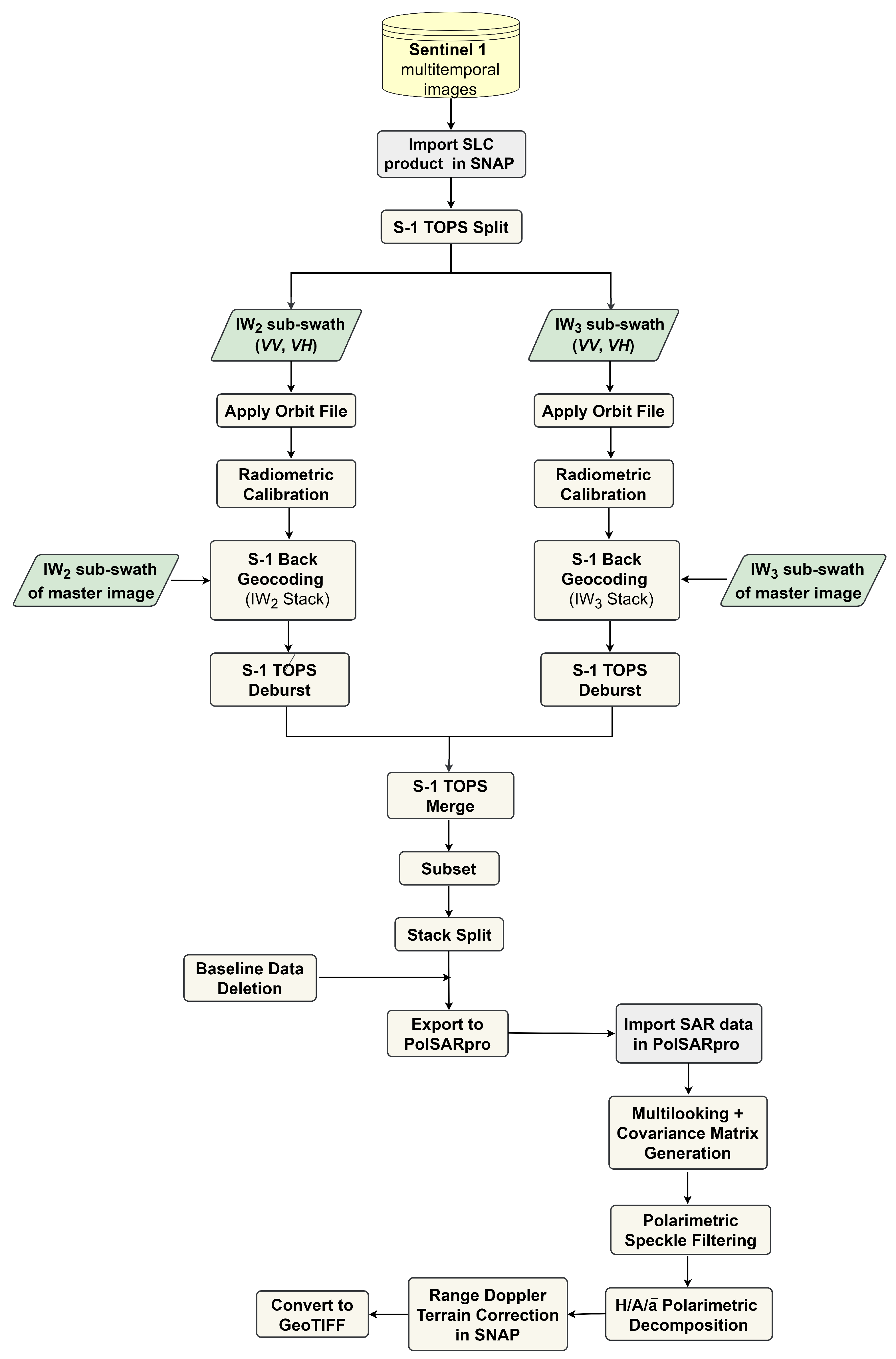
2.3.1. Sentinel-1 Data
2.3.2. Polarimetric Data Representation
2.3.3. Sentinel-2 Data
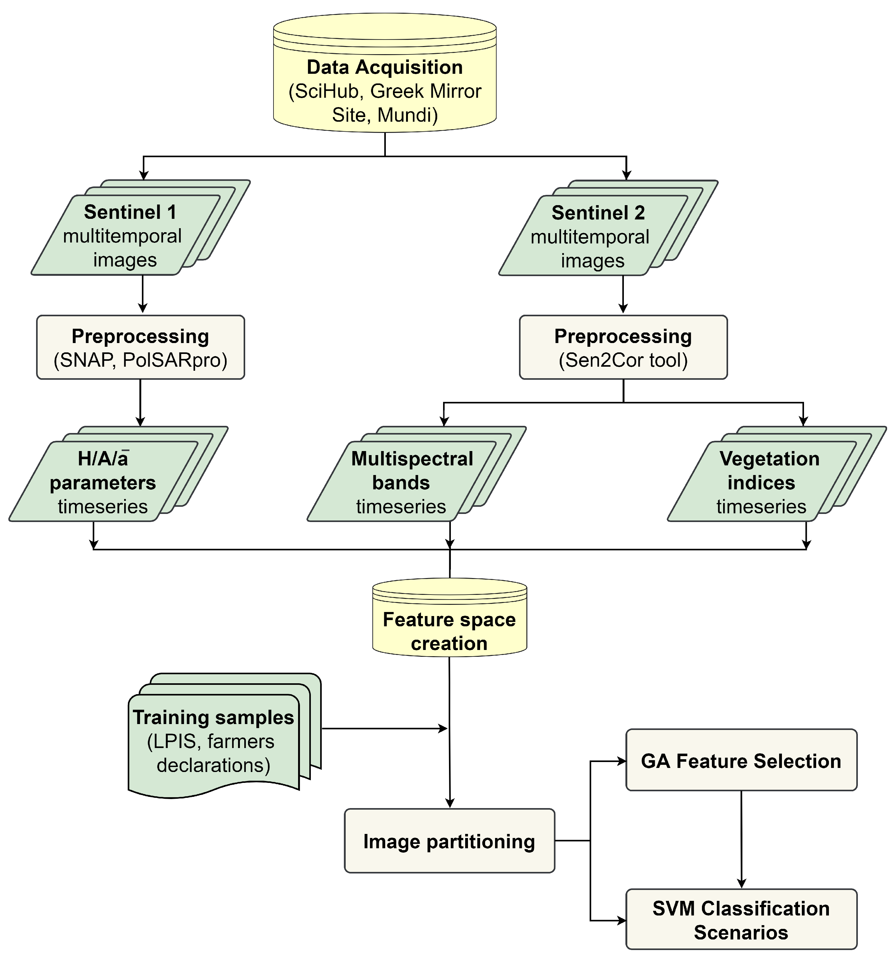
3. Methods
3.1. Image Partitioning and Feature Space Creation
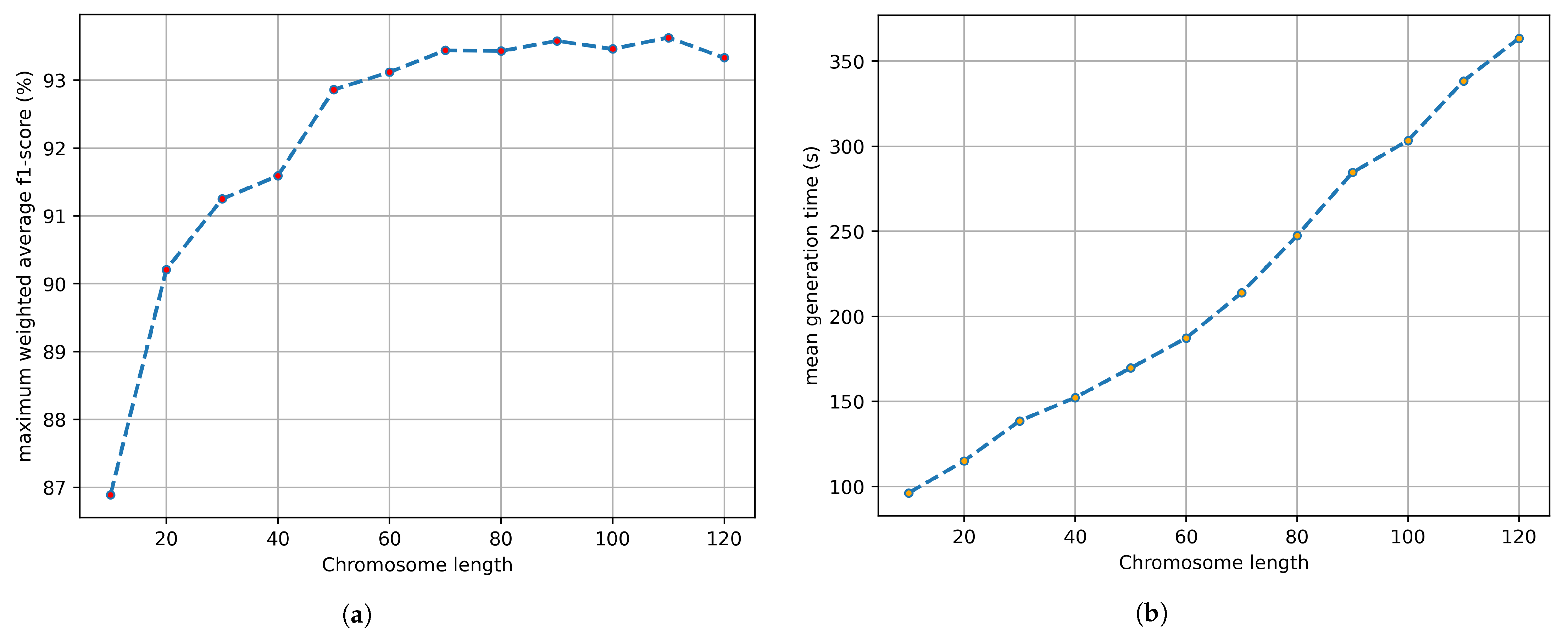
3.2. Genetic Algorithm
3.3. Crop Classification
4. Results
4.1. Crop Classification Results

| Method | UA | PA | f1-Score | OA |
|---|---|---|---|---|
| S2 | 91.06 | 88.95 | 89.93 | 92.42 |
| S1 | 76.10 | 67.68 | 71.12 | 82.83 |
| S1/S2 | 91.09 | 87.99 | 89.41 | 92.28 |
| GA | 91.85 | 90.04 | 90.85 | 93.58 |
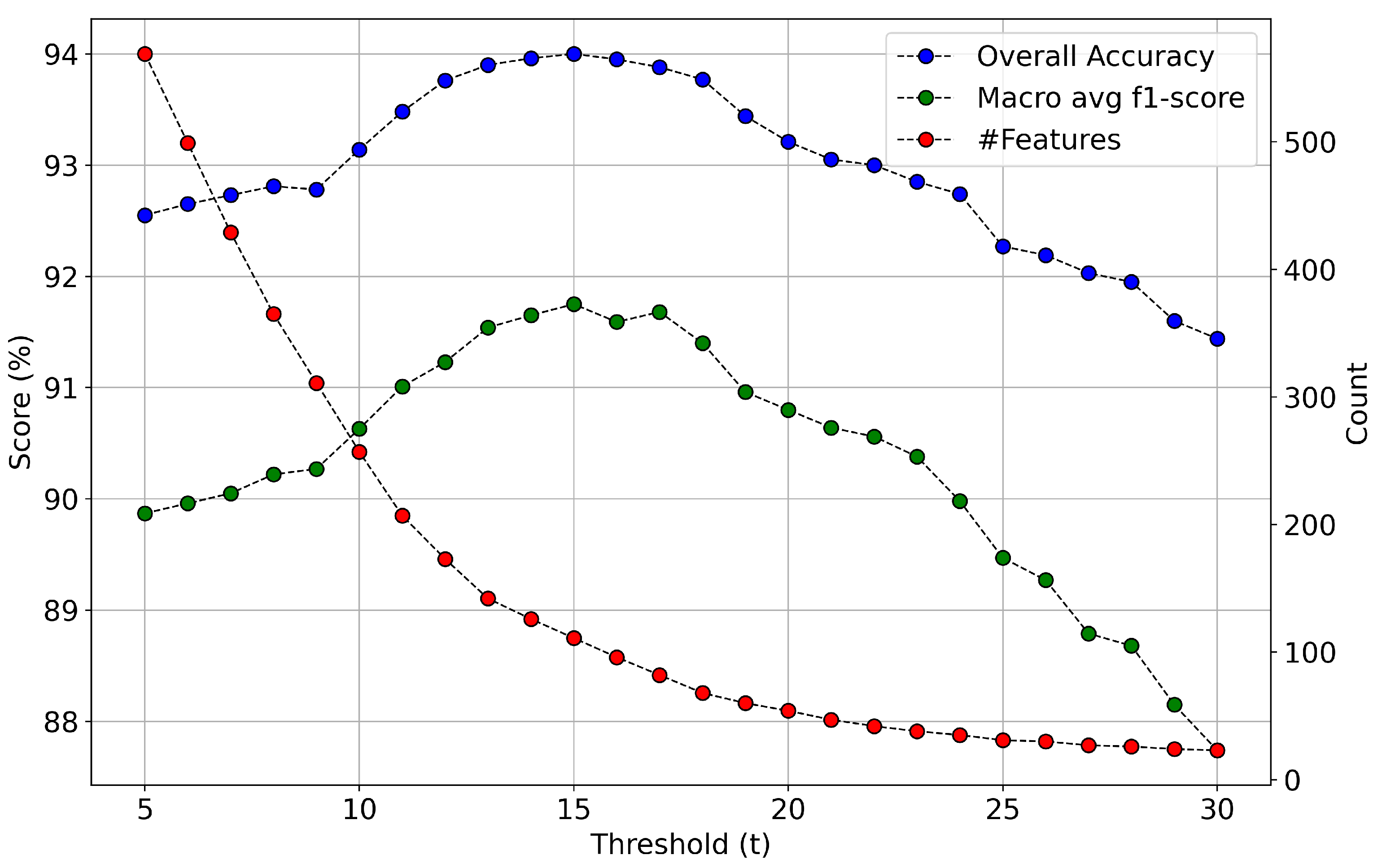
| GA15 | 92.75 | 90.93 | 91.75 | 94.00 |
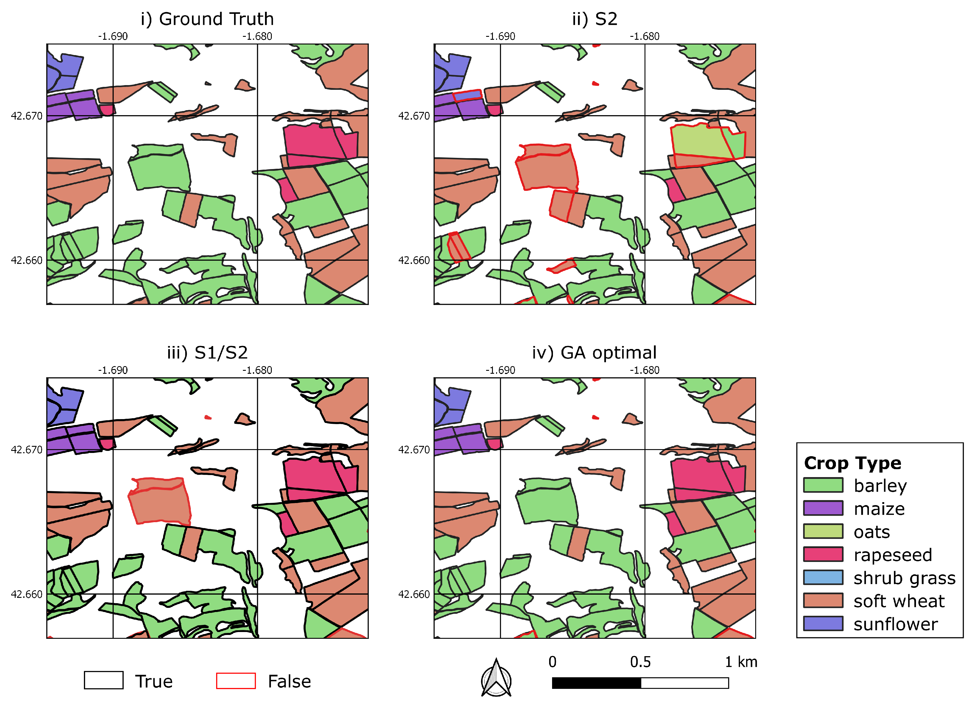
4.1.1. Crop Classification Results Based on Sentinel-2 Imagery (S2 Model)
4.1.2. Crop Classification Results Based on the Combination of Sentinel-1 and Sentinel-2 Multi-Temporal Imagery (S1/S2 Model)
4.1.3. Crop Classification Results Based on Sentinel-1 PolSAR Imagery (S1 Model)
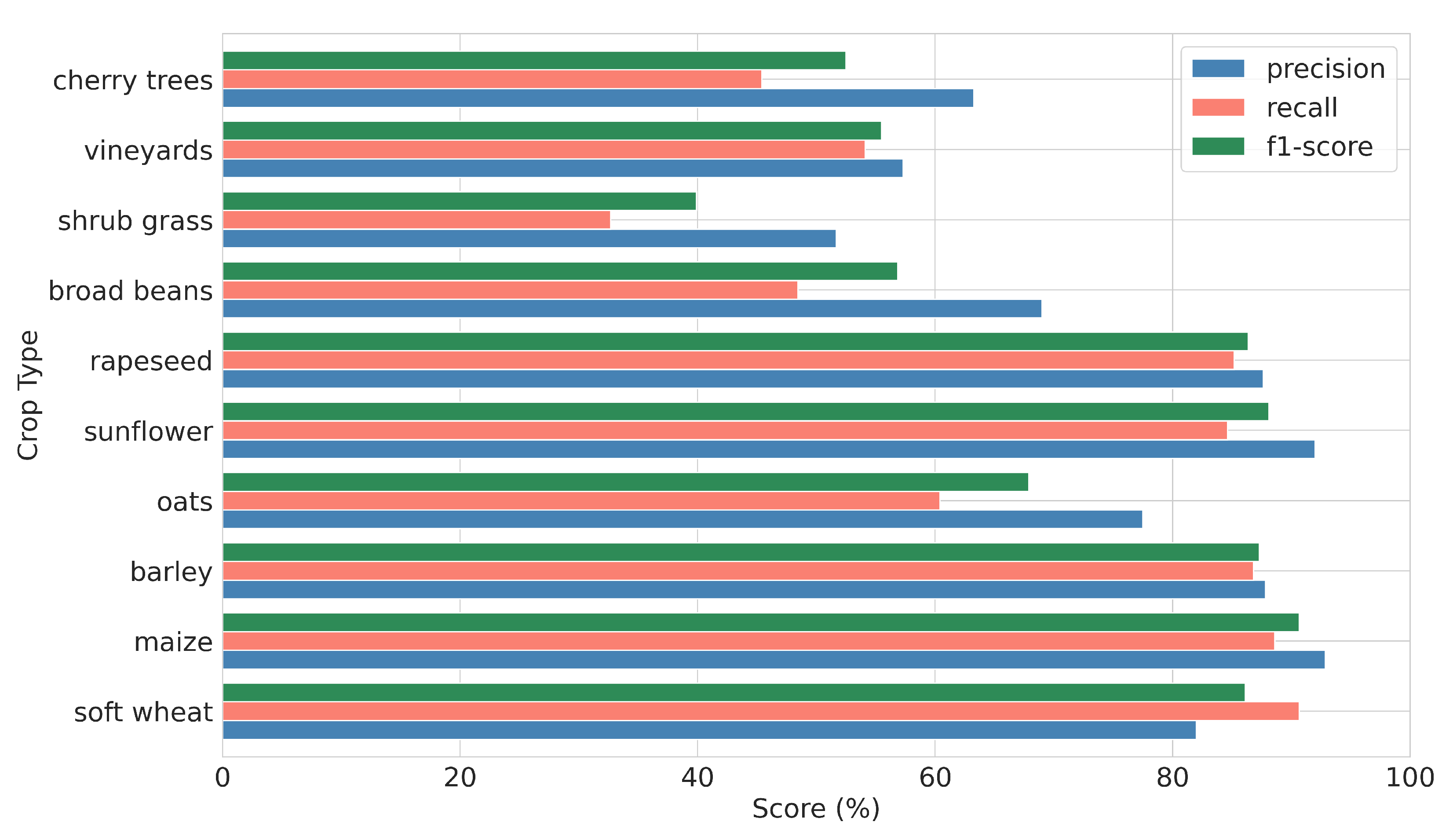
4.1.4. Crop Classification Results Based on Genetic Algorithm’s Results (GA Model)
| Crop Type | UA | PA | f1-Score | Support |
|---|---|---|---|---|
| soft wheat | 94.55 | 95.92 | 95.23 | 3823 |
| maize | 95.04 | 96.22 | 95.60 | 156 |
| barley | 93.84 | 94.35 | 94.10 | 2526 |
| oats | 93.70 | 89.13 | 91.35 | 820 |
| sunflower | 97.55 | 92.35 | 94.86 | 200 |
| rapeseed | 96.17 | 94.80 | 95.47 | 496 |
| broad beans | 95.83 | 90.48 | 93.06 | 147 |
| shrub grass | 85.67 | 81.84 | 83.69 | 228 |
| vineyards | 85.00 | 91.92 | 88.27 | 146 |
| cherry trees | 90.17 | 82.25 | 85.90 | 89 |
| macro avg | 92.75 | 90.93 | 91.75 | 8631 |
| weighted avg | 94.01 | 94.00 | 93.98 | 8631 |
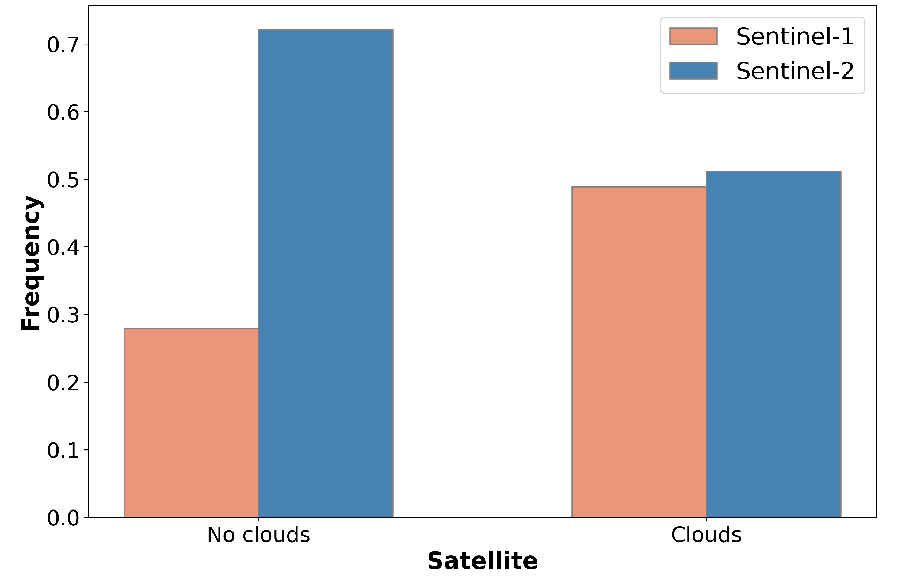
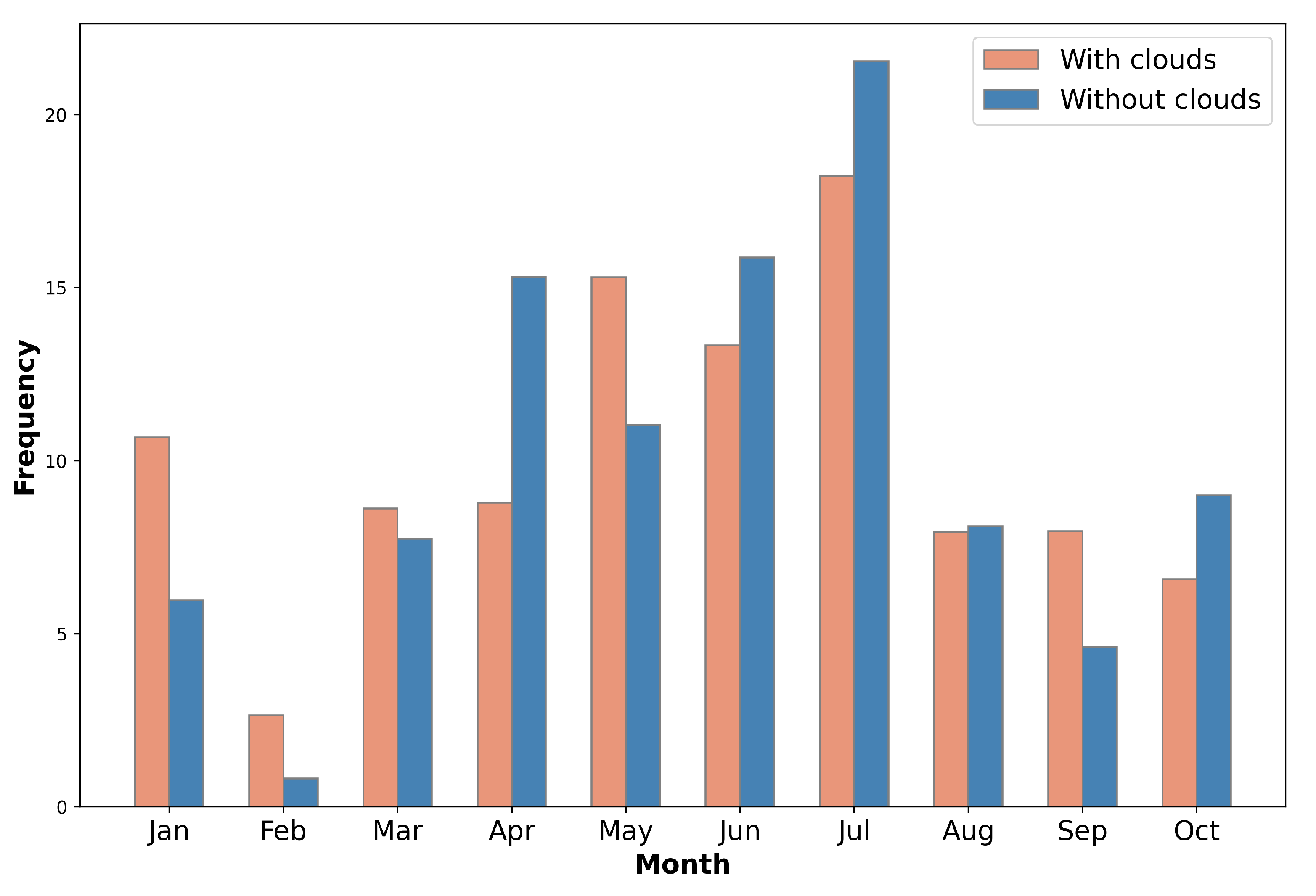
4.2. Performance of Crop Classification Models in Artificially Generated Cloudy Conditions
| f1-Score (%) | PA (%) | UA (%) | |||||||
|---|---|---|---|---|---|---|---|---|---|
| Crop | S2c | S1/S2c | GAc,15 | S2c | S1/S2c | GAc,15 | S2c | S1/S2c | GAc,15 |
| wheat | 88.38 | 90.91 | 92.16 | 91.08 | 93.65 | 94.22 | 85.84 | 88.34 | 90.19 |
| maize | 90.60 | 94.02 | 93.88 | 89.23 | 93.40 | 92.88 | 92.16 | 94.72 | 94.93 |
| barley | 85.83 | 90.51 | 91.51 | 85.08 | 90.04 | 91.02 | 86.60 | 90.99 | 92.01 |
| oats | 76.57 | 81.30 | 84.70 | 71.98 | 75.09 | 80.23 | 81.83 | 88.65 | 89.72 |
| sunflower | 87.31 | 91.67 | 92.50 | 86.50 | 88.75 | 89.45 | 88.22 | 94.85 | 95.78 |
| rapeseed | 84.83 | 91.40 | 92.84 | 81.75 | 89.21 | 92.24 | 88.17 | 93.73 | 93.48 |
| broad bean | 78.97 | 82.23 | 86.98 | 72.11 | 76.26 | 82.11 | 87.81 | 89.36 | 92.55 |
| shrub grass | 72.55 | 73.83 | 76.36 | 68.68 | 70.79 | 72.68 | 77.00 | 77.28 | 80.50 |
| vineyards | 77.99 | 80.34 | 83.33 | 79.11 | 84.52 | 85.62 | 85.62 | 76.71 | 81.23 |
| cherry trees | 76.32 | 78.40 | 83.78 | 75.96 | 71.91 | 82.02 | 76.99 | 86.45 | 85.72 |
| macro | 81.94 | 85.46 | 87.80 | 80.15 | 83.36 | 86.25 | 84.19 | 88.11 | 89.61 |
| weighted | 85.44 | 89.08 | 90.60 | 85.56 | 89.18 | 90.66 | 85.55 | 89.23 | 90.67 |
5. Discussion
5.1. Relevance of Sentinel-1 PolSAR Data for Crop Classification
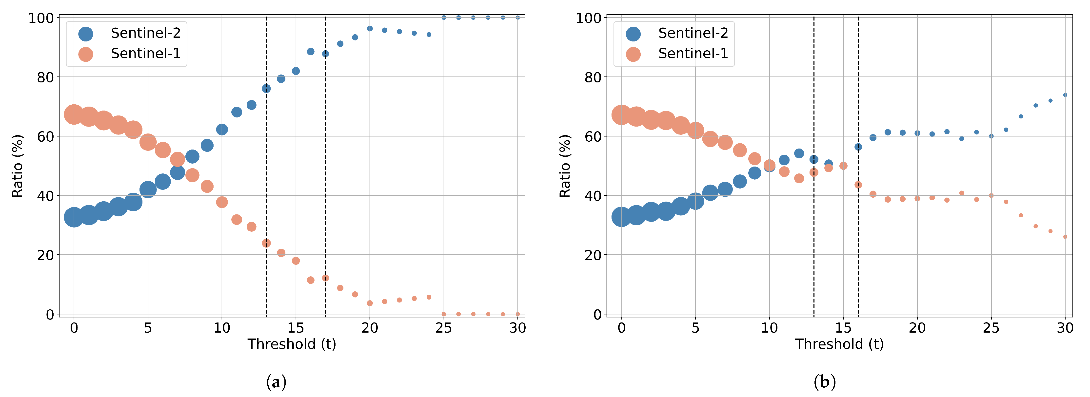
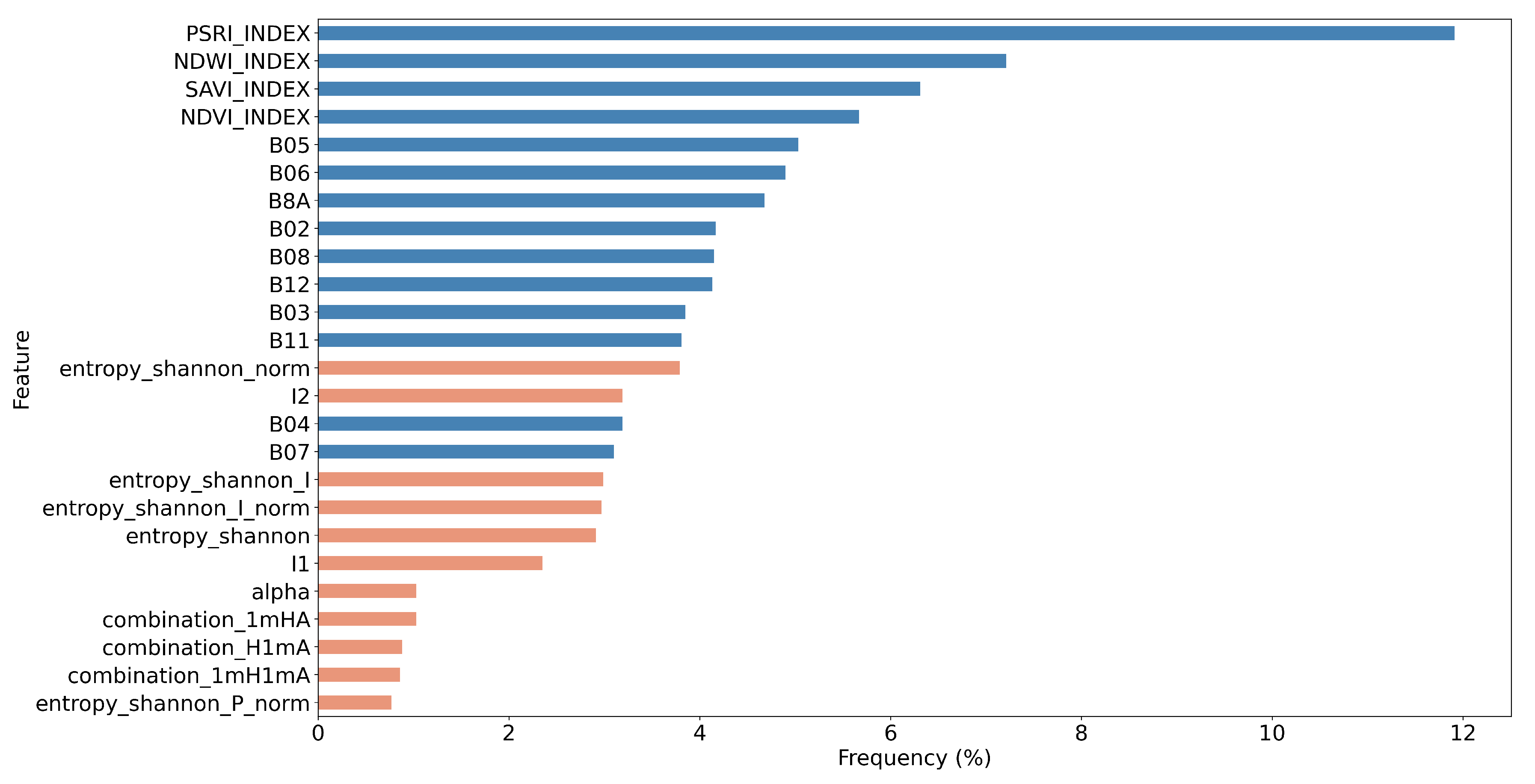
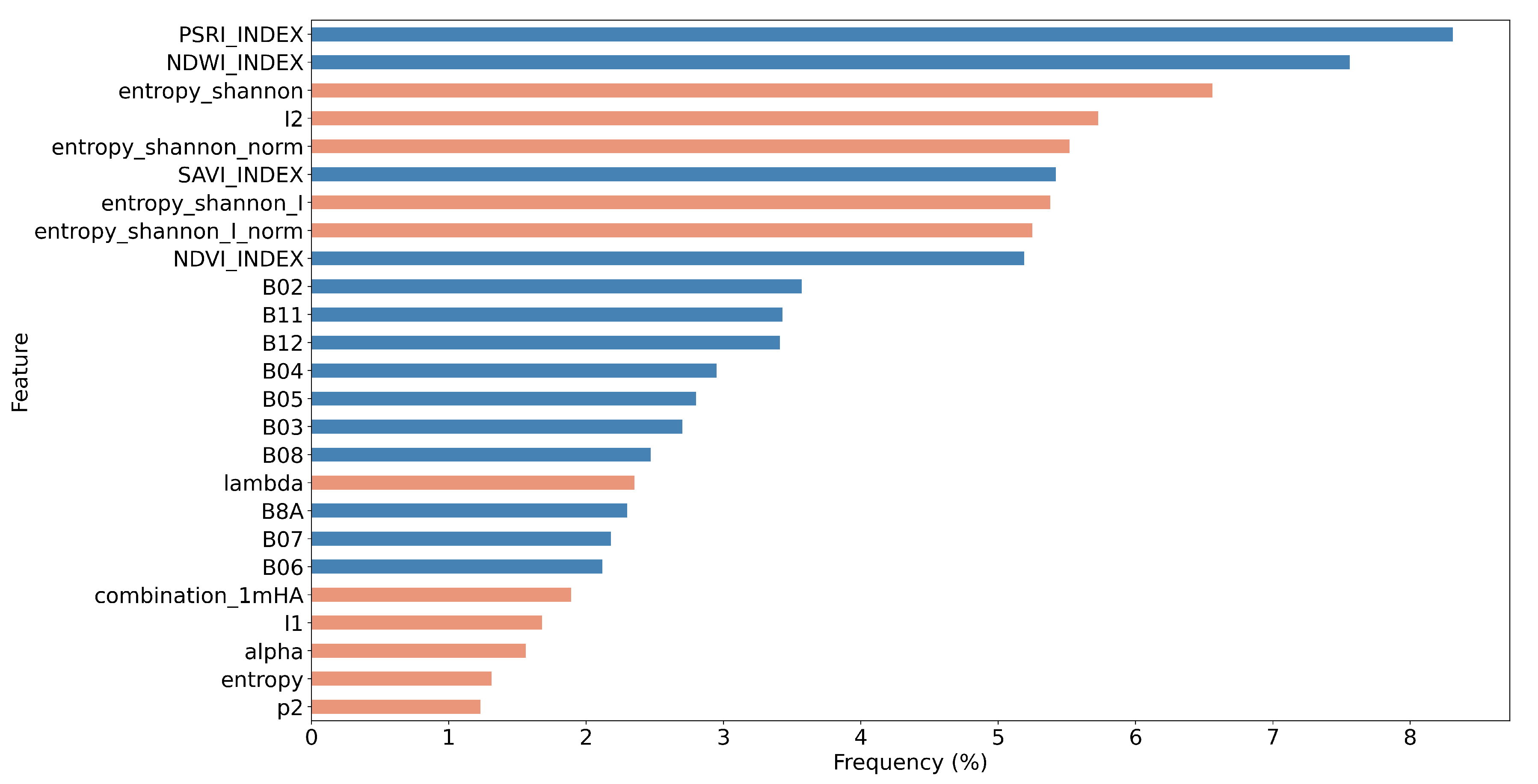
5.2. Feature Importance of the Combined Sentinel-1/2 Feature Space
5.3. Comparison of the GA with Other Feature Selection Methods
5.4. Limitations
6. Conclusions
- The use of all the available optical and polarimetric features improved slightly the crop classification accuracy. However, when artificial cloud masks were injected into the original Sentinel-2 imagery, simulating a real world scenario, the added value of PolSAR data was revealed. The corresponding polarimetric/optical synergistic SVM model presented an accuracy improvement of more than 3.5%, in comparison with the optical-based model under artificially cloudy conditions. This experimental result showcases the potential value of this approach in relevant tasks above agricultural regions that suffer from frequent cloud cover.
- By employing our custom GA, we re-identified the most important features in the scenario of artificial clouds and used them an input data in the SVM classifier. This particular model exhibited an increased OA by 1.5%, approaching 90.66%.
- Through a computationally demanding feature importance estimation analysis of carrying out more than 100 GA experiments, we derived a sorted list of the most important individual predictors in both scenarios of the original cloud-free Sentinel-2 dataset and the one with the artificial cloud masks that could be effectively utilized in future studies. This feature importance analysis verified the great contribution of Sentinel-2 attributes in the original case, as expected, and highlighted the great relative importance of several polarimetric SAR parameters, such as Shannon entropy, especially in the case of injecting artificial cloud coverage.
Supplementary Materials
Author Contributions
Funding
Acknowledgments
Conflicts of Interest
References
- Larrañaga, A.; Álvarez-Mozos, J. On the added value of quad-pol data in a multi-temporal crop classification framework based on RADARSAT-2 imagery. Remote Sens. 2016, 8, 335. [Google Scholar] [CrossRef]
- Orynbaikyzy, A.; Gessner, U.; Conrad, C. Crop type classification using a combination of optical and radar remote sensing data: A review. Int. J. Remote Sens. 2019, 40, 6553–6595. [Google Scholar] [CrossRef]
- Dakir, A.; Alami, O.B.; Barramou, F. Crop type mapping using optical and radar images: A review. In Proceedings of the 2020 IEEE International conference of Moroccan Geomatics (Morgeo), Casablanca, Morocco, 11–13 May 2020; pp. 1–8. [Google Scholar]
- Sonobe, R.; Tani, H.; Wang, X.; Kobayashi, N.; Shimamura, H. Discrimination of crop types with TerraSAR-X-derived information. Phys. Chem. Earth Parts A/B/C 2015, 83, 2–13. [Google Scholar] [CrossRef]
- Giannarakis, G.; Sitokonstantinou, V.; Lorilla, R.S.; Kontoes, C. Towards assessing agricultural land suitability with causal machine learning. In Proceedings of the 2022 IEEE/CVF Conference on Computer Vision and Pattern Recognition Workshops (CVPRW), New Orleans, LA, USA, 19–20 June 2022; pp. 1442–1452. [Google Scholar]
- Sishodia, R.P.; Ray, R.L.; Singh, S.K. Applications of remote sensing in precision agriculture: A review. Remote Sens. 2020, 12, 3136. [Google Scholar] [CrossRef]
- Phiri, D.; Simwanda, M.; Salekin, S.; Nyirenda, V.R.; Murayama, Y.; Ranagalage, M. Sentinel-2 data for land cover/use mapping: A review. Remote Sens. 2020, 12, 2291. [Google Scholar] [CrossRef]
- Campos-Taberner, M.; García-Haro, F.J.; Martínez, B.; Sánchez-Ruíz, S.; Gilabert, M.A. A copernicus Sentinel-1 and Sentinel-2 classification framework for the 2020+ European common agricultural policy: A case study in València (Spain). Agronomy 2019, 9, 556. [Google Scholar] [CrossRef]
- Beriaux, E.; Jago, A.; Lucau-Danila, C.; Planchon, V.; Defourny, P. Sentinel-1 Time Series for Crop Identification in the Framework of the Future CAP Monitoring. Remote Sens. 2021, 13, 2785. [Google Scholar] [CrossRef]
- Hunt, M.L.; Blackburn, G.A.; Carrasco, L.; Redhead, J.W.; Rowland, C.S. High resolution wheat yield mapping using Sentinel-2. Remote Sens. Environ. 2019, 233, 111410. [Google Scholar] [CrossRef]
- Nasirzadehdizaji, R.; Balik Sanli, F.; Abdikan, S.; Cakir, Z.; Sekertekin, A.; Ustuner, M. Sensitivity analysis of multi-temporal Sentinel-1 SAR parameters to crop height and canopy coverage. Appl. Sci. 2019, 9, 655. [Google Scholar] [CrossRef]
- Torres, R.; Snoeij, P.; Geudtner, D.; Bibby, D.; Davidson, M.; Attema, E.; Potin, P.; Rommen, B.; Floury, N.; Brown, M.; et al. GMES Sentinel-1 mission. Remote Sens. Environ. 2012, 120, 9–24. [Google Scholar] [CrossRef]
- Raspini, F.; Bianchini, S.; Ciampalini, A.; Del Soldato, M.; Solari, L.; Novali, F.; Del Conte, S.; Rucci, A.; Ferretti, A.; Casagli, N. Continuous, semi-automatic monitoring of ground deformation using Sentinel-1 satellites. Sci. Rep. 2018, 8, 7253. [Google Scholar] [CrossRef]
- Van Tricht, K.; Gobin, A.; Gilliams, S.; Piccard, I. Synergistic use of radar Sentinel-1 and optical Sentinel-2 imagery for crop mapping: A case study for Belgium. Remote Sens. 2018, 10, 1642. [Google Scholar] [CrossRef]
- Lechner, A.M.; Foody, G.M.; Boyd, D.S. Applications in remote sensing to forest ecology and management. One Earth 2020, 2, 405–412. [Google Scholar] [CrossRef]
- Gao, H.; Wang, C.; Wang, G.; Zhu, J.; Tang, Y.; Shen, P.; Zhu, Z. A crop classification method integrating GF-3 PolSAR and Sentinel-2A optical data in the Dongting Lake Basin. Sensors 2018, 18, 3139. [Google Scholar] [CrossRef]
- Kobayashi, N.; Tani, H.; Wang, X.; Sonobe, R. Crop classification using spectral indices derived from Sentinel-2A imagery. J. Inf. Telecommun. 2020, 4, 67–90. [Google Scholar] [CrossRef]
- Mazzia, V.; Khaliq, A.; Chiaberge, M. Improvement in land cover and crop classification based on temporal features learning from Sentinel-2 data using recurrent-convolutional neural network (R-CNN). Appl. Sci. 2019, 10, 238. [Google Scholar] [CrossRef]
- Sitokonstantinou, V.; Papoutsis, I.; Kontoes, C.; Lafarga Arnal, A.; Armesto Andrés, A.P.; Garraza Zurbano, J.A. Scalable parcel-based crop identification scheme using Sentinel-2 data time-series for the monitoring of the common agricultural policy. Remote Sens. 2018, 10, 911. [Google Scholar] [CrossRef]
- Sitokonstantinou, V.; Koukos, A.; Drivas, T.; Kontoes, C.; Papoutsis, I.; Karathanassi, V. A Scalable Machine Learning Pipeline for Paddy Rice Classification Using Multi-Temporal Sentinel Data. Remote Sens. 2021, 13, 1769. [Google Scholar] [CrossRef]
- Sitokonstantinou, V.; Drivas, T.; Koukos, A.; Papoutsis, I.; Kontoes, C. Scalable distributed random forest classification for paddy rice mapping. Zenodo 2020, 11. [Google Scholar] [CrossRef]
- Yi, Z.; Jia, L.; Chen, Q. Crop classification using multi-temporal Sentinel-2 data in the Shiyang River Basin of China. Remote Sens. 2020, 12, 4052. [Google Scholar] [CrossRef]
- Rußwurm, M.; Körner, M. Multi-temporal land cover classification with sequential recurrent encoders. ISPRS Int. J. Geo-Inf. 2018, 7, 129. [Google Scholar] [CrossRef]
- Jiang, Y.; Lu, Z.; Li, S.; Lei, Y.; Chu, Q.; Yin, X.; Chen, F. Large-scale and high-resolution crop mapping in china using Sentinel-2 satellite imagery. Agriculture 2020, 10, 433. [Google Scholar] [CrossRef]
- Chen, Y.; Lu, D.; Moran, E.; Batistella, M.; Dutra, L.V.; Sanches, I.D.; da Silva, R.F.B.; Huang, J.; Luiz, A.J.B.; de Oliveira, M.A.F. Mapping croplands, cropping patterns, and crop types using MODIS time-series data. Int. J. Appl. Earth Obs. Geoinf. 2018, 69, 133–147. [Google Scholar] [CrossRef]
- Liu, C.a.; Chen, Z.X.; Yun, S.; Chen, J.s.; Hasi, T.; PAN, H.z. Research advances of SAR remote sensing for agriculture applications: A review. J. Integr. Agric. 2019, 18, 506–525. [Google Scholar] [CrossRef]
- Valcarce-Diñeiro, R.; Arias-Pérez, B.; Lopez-Sanchez, J.M.; Sánchez, N. Multi-temporal dual-and quad-polarimetric synthetic aperture radar data for crop-type mapping. Remote Sens. 2019, 11, 1518. [Google Scholar] [CrossRef]
- Mandal, D.; Kumar, V.; Ratha, D.; Dey, S.; Bhattacharya, A.; Lopez-Sanchez, J.M.; McNairn, H.; Rao, Y.S. Dual polarimetric radar vegetation index for crop growth monitoring using Sentinel-1 SAR data. Remote Sens. Environ. 2020, 247, 111954. [Google Scholar] [CrossRef]
- Arias, M.; Campo-Bescós, M.Á.; Álvarez-Mozos, J. Crop classification based on temporal signatures of Sentinel-1 observations over Navarre province, Spain. Remote Sens. 2020, 12, 278. [Google Scholar] [CrossRef]
- Mestre-Quereda, A.; Lopez-Sanchez, J.M.; Vicente-Guijalba, F.; Jacob, A.W.; Engdahl, M.E. Time-series of Sentinel-1 interferometric coherence and backscatter for crop-type mapping. IEEE J. Sel. Top. Appl. Earth Obs. Remote Sens. 2020, 13, 4070–4084. [Google Scholar] [CrossRef]
- Zhu, X.X.; Montazeri, S.; Ali, M.; Hua, Y.; Wang, Y.; Mou, L.; Shi, Y.; Xu, F.; Bamler, R. Deep learning meets SAR: Concepts, models, pitfalls, and perspectives. IEEE Geosci. Remote Sens. Mag. 2021, 9, 143–172. [Google Scholar] [CrossRef]
- Qu, Y.; Zhao, W.; Yuan, Z.; Chen, J. Crop Mapping from Sentinel-1 Polarimetric Time-Series with a Deep Neural Network. Remote Sens. 2020, 12, 2493. [Google Scholar] [CrossRef]
- Lee, J.S.; Pottier, E. Polarimetric Radar Imaging: From Basics to Applications; CRC Press: Boca Raton, FL, USA, 2017. [Google Scholar]
- Ustuner, M.; Balik Sanli, F. Polarimetric target decompositions and light gradient boosting machine for crop classification: A comparative evaluation. ISPRS Int. J. Geo-Inf. 2019, 8, 97. [Google Scholar] [CrossRef]
- Cloude, S.R.; Pottier, E. An entropy based classification scheme for land applications of polarimetric SAR. IEEE Trans. Geosci. Remote Sens. 1997, 35, 68–78. [Google Scholar] [CrossRef]
- Zeyada, H.H.; Ezz, M.M.; Nasr, A.H.; Shokr, M.; Harb, H.M. Evaluation of the discrimination capability of full polarimetric SAR data for crop classification. Int. J. Remote Sens. 2016, 37, 2585–2603. [Google Scholar] [CrossRef]
- Cloude, S. The dual polarization entropy/alpha decomposition: A PALSAR case study. Sci. Appl. SAR Polarim. Polarim. Interferom. 2007, 644, 2. [Google Scholar]
- Ouchi, K. Recent trend and advance of synthetic aperture radar with selected topics. Remote Sens. 2013, 5, 716–807. [Google Scholar] [CrossRef]
- López-Martínez, C.; Pottier, E. Basic principles of SAR polarimetry. In Polarimetric Synthetic Aperture Radar; Springer: Berlin/Heidelberg, Germany, 2021; pp. 1–58. [Google Scholar]
- Pottier, E.; Sarti, F.; Fitrzyk, M.; Patruno, J. PolSARpro-Biomass Edition: The new ESA polarimetric SAR data processing and educational toolbox for the future ESA & third party fully polarimetric SAR missions. In Proceedings of the ESA Living Planet Symposium 2019, Milan, Italy, 13–17 May 2019. [Google Scholar]
- Morio, J.; Réfrégier, P.; Goudail, F.; Dubois-Fernandez, P.; Dupuis, X. Application of information theory measures to polarimetric and interferometric SAR images. In Proceedings of the PSIP 2007—5th International Conference on Physics in Signal & Image Processing, Mulhouse, France, 30 January–2 February 2007. [Google Scholar]
- Li, M.; Bijker, W. Vegetable classification in Indonesia using Dynamic Time Warping of Sentinel-1A dual polarization SAR time series. Int. J. Appl. Earth Obs. Geoinf. 2019, 78, 268–280. [Google Scholar] [CrossRef]
- Sayedain, S.A.; Maghsoudi, Y.; Eini-Zinab, S. Assessing the use of cross-orbit Sentinel-1 images in land cover classification. Int. J. Remote Sens. 2020, 41, 7801–7819. [Google Scholar] [CrossRef]
- Diniz, J.M.F.d.S.; Gama, F.F.; Adami, M. Evaluation of polarimetry and interferometry of Sentinel-1A SAR data for land use and land cover of the Brazilian Amazon Region. Geocarto Int. 2022, 37, 1482–1500. [Google Scholar] [CrossRef]
- Whyte, A.; Ferentinos, K.P.; Petropoulos, G.P. A new synergistic approach for monitoring wetlands using Sentinels-1 and 2 data with object-based machine learning algorithms. Environ. Model. Softw. 2018, 104, 40–54. [Google Scholar] [CrossRef]
- Hu, J.; Ghamisi, P.; Zhu, X.X. Feature extraction and selection of Sentinel-1 dual-pol data for global-scale local climate zone classification. ISPRS Int. J. Geo-Inf. 2018, 7, 379. [Google Scholar] [CrossRef]
- Schulz, D.; Yin, H.; Tischbein, B.; Verleysdonk, S.; Adamou, R.; Kumar, N. Land use mapping using Sentinel-1 and Sentinel-2 time series in a heterogeneous landscape in Niger, Sahel. ISPRS J. Photogramm. Remote Sens. 2021, 178, 97–111. [Google Scholar] [CrossRef]
- Harfenmeister, K.; Itzerott, S.; Weltzien, C.; Spengler, D. Agricultural monitoring using polarimetric decomposition parameters of Sentinel-1 data. Remote Sens. 2021, 13, 575. [Google Scholar] [CrossRef]
- Mercier, A.; Betbeder, J.; Baudry, J.; Le Roux, V.; Spicher, F.; Lacoux, J.; Roger, D.; Hubert-Moy, L. Evaluation of Sentinel-1 & 2 time series for predicting wheat and rapeseed phenological stages. ISPRS J. Photogramm. Remote Sens. 2020, 163, 231–256. [Google Scholar]
- Haldar, D.; Verma, A.; Kumar, S.; Chauhan, P. Estimation of mustard and wheat phenology using multi-date Shannon entropy and Radar Vegetation Index from polarimetric Sentinel-1. Geocarto Int. 2021, 37, 1–22. [Google Scholar] [CrossRef]
- Yeasin, M.; Haldar, D.; Kumar, S.; Paul, R.K.; Ghosh, S. Machine Learning Techniques for Phenology Assessment of Sugarcane Using Conjunctive SAR and Optical Data. Remote Sens. 2022, 14, 3249. [Google Scholar] [CrossRef]
- Mercier, A.; Betbeder, J.; Rapinel, S.; Jegou, N.; Baudry, J.; Hubert-Moy, L. Evaluation of Sentinel-1 and-2 time series for estimating LAI and biomass of wheat and rapeseed crop types. J. Appl. Remote Sens. 2020, 14, 024512. [Google Scholar] [CrossRef]
- Umutoniwase, N.; Lee, S.K. The Potential of Sentinel-1 SAR Parameters in Monitoring Rice Paddy Phenological Stages in Gimhae, South Korea. Korean J. Remote Sens. 2021, 37, 789–802. [Google Scholar]
- Hosseini, M.; Becker-Reshef, I.; Sahajpal, R.; Lafluf, P.; Leale, G.; Puricelli, E.; Skakun, S.; McNairn, H. Soybean Yield Forecast Using Dual-Polarimetric C-Band Synthetic Aperture Radar. ISPRS Ann. Photogramm. Remote Sens. Spat. Inf. Sci. 2022, 3, 405–410. [Google Scholar] [CrossRef]
- De Petris, S.; Sarvia, F.; Gullino, M.; Tarantino, E.; Borgogno-Mondino, E. Sentinel-1 polarimetry to map apple orchard damage after a storm. Remote Sens. 2021, 13, 1030. [Google Scholar] [CrossRef]
- Elkharrouba, E.; Sekertekin, A.; Fathi, J.; Tounsi, Y.; Bioud, H.; Nassim, A. Surface soil moisture estimation using dual-Polarimetric Stokes parameters and backscattering coefficient. Remote Sens. Appl. Soc. Environ. 2022, 26, 100737. [Google Scholar] [CrossRef]
- Tavus, B.; Kocaman, S.; Nefeslioglu, H.; Gokceoglu, C. A fusion approach for flood mapping using Sentinel-1 and Sentinel-2 datasets. Int. Arch. Photogramm. Remote Sens. Spat. Inf. Sci. 2020, 43, 641–648. [Google Scholar] [CrossRef]
- Parida, B.R.; Mandal, S.P. Polarimetric decomposition methods for LULC mapping using ALOS L-band PolSAR data in Western parts of Mizoram, Northeast India. SN Appl. Sci. 2020, 2, 1049. [Google Scholar] [CrossRef]
- Wang, D.; Liu, C.A.; Zeng, Y.; Tian, T.; Sun, Z. Dryland Crop Classification Combining Multitype Features and Multitemporal Quad-Polarimetric RADARSAT-2 Imagery in Hebei Plain, China. Sensors 2021, 21, 332. [Google Scholar] [CrossRef]
- Sun, Z.; Wang, D.; Zhong, G. A review of crop classification using satellite-based polarimetric SAR imagery. In Proceedings of the 2018 7th International Conference on Agro-Geoinformatics (Agro-Geoinformatics), Hangzhou, China, 6–9 August 2018; pp. 1–5. [Google Scholar]
- Guo, J.; Wei, P.L.; Liu, J.; Jin, B.; Su, B.F.; Zhou, Z.S. Crop Classification Based on Differential Characteristics of H/α Scattering Parameters for Multitemporal Quad-and Dual-Polarization SAR Images. IEEE Trans. Geosci. Remote Sens. 2018, 56, 6111–6123. [Google Scholar] [CrossRef]
- Kpienbaareh, D.; Sun, X.; Wang, J.; Luginaah, I.; Bezner Kerr, R.; Lupafya, E.; Dakishoni, L. Crop type and land cover mapping in northern Malawi using the integration of Sentinel-1, Sentinel-2, and planetscope satellite data. Remote Sens. 2021, 13, 700. [Google Scholar] [CrossRef]
- Denize, J.; Hubert-Moy, L.; Pottier, E. Polarimetric SAR time-series for identification of winter land use. Sensors 2019, 19, 5574. [Google Scholar] [CrossRef]
- Gella, G.W.; Bijker, W.; Belgiu, M. Mapping crop types in complex farming areas using SAR imagery with dynamic time warping. ISPRS J. Photogramm. Remote Sens. 2021, 175, 171–183. [Google Scholar] [CrossRef]
- Gao, H.; Wang, C.; Wang, G.; Li, Q.; Zhu, J. A new crop classification method based on the time-varying feature curves of time series dual-polarization Sentinel-1 data sets. IEEE Geosci. Remote Sens. Lett. 2019, 17, 1183–1187. [Google Scholar] [CrossRef]
- Oldoni, L.; Prudente, V.; Diniz, J.; Wiederkehr, N.; Sanches, I.; Gama, F. Polarimetric Sar Data from Sentinel-1A Applied to Early Crop Classification. Int. Arch. Photogramm. Remote Sens. Spat. Inf. Sci. 2020, 43, 1039–1046. [Google Scholar] [CrossRef]
- Gao, H.; Wang, C.; Wang, G.; Fu, H.; Zhu, J. A novel crop classification method based on ppfSVM classifier with time-series alignment kernel from dual-polarization SAR datasets. Remote Sens. Environ. 2021, 264, 112628. [Google Scholar] [CrossRef]
- Chabalala, Y.; Adam, E.; Ali, K.A. Machine Learning Classification of Fused Sentinel-1 and Sentinel-2 Image Data towards Mapping Fruit Plantations in Highly Heterogenous Landscapes. Remote Sens. 2022, 14, 2621. [Google Scholar] [CrossRef]
- Yaping, D.; Zhongxin, C. A review of crop identification and area monitoring based on SAR image. In Proceedings of the 2012 First International Conference on Agro-Geoinformatics (Agro-Geoinformatics), Shanghai, China, 2–4 August 2012; pp. 1–4. [Google Scholar]
- Chakhar, A.; Hernández-López, D.; Ballesteros, R.; Moreno, M.A. Improving the accuracy of multiple algorithms for crop classification by integrating Sentinel-1 observations with Sentinel-2 data. Remote Sens. 2021, 13, 243. [Google Scholar] [CrossRef]
- David, N.; Giordano, S.; Mallet, C. Investigating operational country-level crop monitoring with Sentinel-1 and -2 imagery. Remote Sens. Lett. 2021, 12, 970–982. [Google Scholar] [CrossRef]
- Kussul, N.; Lavreniuk, M.; Shumilo, L. Deep Recurrent Neural Network for Crop Classification Task Based on Sentinel-1 and Sentinel-2 Imagery. In Proceedings of the IGARSS 2020–2020 IEEE International Geoscience and Remote Sensing Symposium, Waikoloa, HI, USA, 26 September–2 October 2020; pp. 6914–6917. [Google Scholar]
- Niculescu Sr, S.; Billey, A.; Talab-Ou-Ali, H., Jr. Random forest classification using Sentinel-1 and Sentinel-2 series for vegetation monitoring in the Pays de Brest (France). In Proceedings of the SPIE Remote Sensing for Agriculture, Ecosystems, and Hydrology XX, Berlin, Germany, 10–13 September 2018; Volume 10783, p. 1078305. [Google Scholar]
- Felegari, S.; Sharifi, A.; Moravej, K.; Amin, M.; Golchin, A.; Muzirafuti, A.; Tariq, A.; Zhao, N. Integration of Sentinel 1 and Sentinel 2 Satellite Images for Crop Mapping. Appl. Sci. 2021, 11, 10104. [Google Scholar] [CrossRef]
- Fundisi, E.; Tesfamichael, S.G.; Ahmed, F. A combination of Sentinel-1 RADAR and Sentinel-2 multispectral data improves classification of morphologically similar savanna woody plants. Eur. J. Remote Sens. 2022, 55, 372–387. [Google Scholar] [CrossRef]
- He, T.; Zhao, K. Multispectral remote sensing land use classification based on RBF neural network with parameters optimized by genetic algorithm. In Proceedings of the 2018 International Conference on Sensor Networks and Signal Processing (SNSP), Xi’an, China, 28–31 October 2018; pp. 118–123. [Google Scholar]
- Chu, H.; Ge, L.; Ng, A.; Rizos, C. Application of genetic algorithm and support vector machine in classification of multisource remote sensing data. Int. J. Remote Sens. Appl. 2012, 2, 1–11. [Google Scholar]
- Zhu, J.; Pan, Z.; Wang, H.; Huang, P.; Sun, J.; Qin, F.; Liu, Z. An improved multi-temporal and multi-feature tea plantation identification method using Sentinel-2 imagery. Sensors 2019, 19, 2087. [Google Scholar] [CrossRef]
- Cui, J.; Zhang, X.; Wang, W.; Wang, L. Integration of optical and SAR remote sensing images for crop-type mapping based on a novel object-oriented feature selection method. Int. J. Agric. Biol. Eng. 2020, 13, 178–190. [Google Scholar] [CrossRef]
- Paul, S.; Kumar, D.N. Evaluation of feature selection and feature extraction techniques on multi-temporal Landsat-8 images for crop classification. Remote Sens. Earth Syst. Sci. 2019, 2, 197–207. [Google Scholar] [CrossRef]
- Blickensdörfer, L.; Schwieder, M.; Pflugmacher, D.; Nendel, C.; Erasmi, S.; Hostert, P. Mapping of crop types and crop sequences with combined time series of Sentinel-1, Sentinel-2 and Landsat 8 data for Germany. Remote Sens. Environ. 2022, 269, 112831. [Google Scholar] [CrossRef]
- Löw, F.; Michel, U.; Dech, S.; Conrad, C. Impact of feature selection on the accuracy and spatial uncertainty of per-field crop classification using support vector machines. ISPRS J. Photogramm. Remote Sens. 2013, 85, 102–119. [Google Scholar] [CrossRef]
- Yin, L.; You, N.; Zhang, G.; Huang, J.; Dong, J. Optimizing feature selection of individual crop types for improved crop mapping. Remote Sens. 2020, 12, 162. [Google Scholar] [CrossRef]
- Wirsansky, E. Hands-On Genetic Algorithms with Python: Applying Genetic Algorithms to Solve Real-World Deep Learning and Artificial Intelligence Problems; Packt Publishing Ltd.: Birmingham, UK, 2020. [Google Scholar]
- Zhi, H.; Liu, S. Face recognition based on genetic algorithm. J. Vis. Commun. Image Represent. 2019, 58, 495–502. [Google Scholar] [CrossRef]
- Kramer, O. Genetic algorithms. In Genetic Algorithm Essentials; Springer: Berlin/Heidelberg, Germany, 2017; pp. 11–19. [Google Scholar]
- Haddadi, G.A.; Reza Sahebi, M.; Mansourian, A. Polarimetric SAR feature selection using a genetic algorithm. Can. J. Remote Sens. 2011, 37, 27–36. [Google Scholar] [CrossRef]
- Li, S.; Wu, H.; Wan, D.; Zhu, J. An effective feature selection method for hyperspectral image classification based on genetic algorithm and support vector machine. Knowl.-Based Syst. 2011, 24, 40–48. [Google Scholar] [CrossRef]
- Shi, L.; Wan, Y.; Gao, X.; Wang, M. Feature selection for object-based classification of high-resolution remote sensing images based on the combination of a genetic algorithm and tabu search. Comput. Intell. Neurosci. 2018, 2018, 6595792. [Google Scholar] [CrossRef]
- Zhou, Y.; Zhang, R.; Wang, S.; Wang, F. Feature selection method based on high-resolution remote sensing images and the effect of sensitive features on classification accuracy. Sensors 2018, 18, 2013. [Google Scholar] [CrossRef]
- Zhuo, L.; Zheng, J.; Li, X.; Wang, F.; Ai, B.; Qian, J. A genetic algorithm based wrapper feature selection method for classification of hyperspectral images using support vector machine. In Proceedings of the Geoinformatics 2008 and Joint Conference on GIS and Built Environment: Classification of Remote Sensing Images, Guangzhou, China, 28–29 June 2008; Volume 7147, pp. 503–511. [Google Scholar]
- Ming, D.; Zhou, T.; Wang, M.; Tan, T. Land cover classification using random forest with genetic algorithm-based parameter optimization. J. Appl. Remote Sens. 2016, 10, 035021. [Google Scholar] [CrossRef]
- Tomppo, E.; Antropov, O.; Praks, J. Cropland classification using Sentinel-1 time series: Methodological performance and prediction uncertainty assessment. Remote Sens. 2019, 11, 2480. [Google Scholar] [CrossRef]
- Zang, S.; Zhang, C.; Zhang, L.; Zhang, Y. Wetland remote sensing classification using support vector machine optimized with genetic algorithm: A case study in Honghe Nature National Reserve. Sci. Geogr. Sin. 2012, 32, 434–441. [Google Scholar]
- Rodriguez-Galiano, V.F.; Ghimire, B.; Rogan, J.; Chica-Olmo, M.; Rigol-Sanchez, J.P. An assessment of the effectiveness of a random forest classifier for land-cover classification. ISPRS J. Photogramm. Remote Sens. 2012, 67, 93–104. [Google Scholar] [CrossRef]
- Rousi, M.; Sitokonstantinou, V.; Meditskos, G.; Papoutsis, I.; Gialampoukidis, I.; Koukos, A.; Karathanassi, V.; Drivas, T.; Vrochidis, S.; Kontoes, C.; et al. Semantically enriched crop type classification and linked earth observation data to support the common agricultural policy monitoring. IEEE J. Sel. Top. Appl. Earth Obs. Remote Sens. 2020, 14, 529–552. [Google Scholar] [CrossRef]
- Vreugdenhil, M.; Wagner, W.; Bauer-Marschallinger, B.; Pfeil, I.; Teubner, I.; Rüdiger, C.; Strauss, P. Sensitivity of Sentinel-1 backscatter to vegetation dynamics: An Austrian case study. Remote Sens. 2018, 10, 1396. [Google Scholar] [CrossRef]
- Ainsworth, T.L.; Kelly, J.; Lee, J.S. Polarimetric analysis of dual polarimetric SAR imagery. In Proceedings of the 7th European Conference on Synthetic Aperture Radar, Friedrichshafen, Germany, 2–5 June 2008; pp. 1–4. [Google Scholar]
- Moreira, A.; Prats-Iraola, P.; Younis, M.; Krieger, G.; Hajnsek, I.; Papathanassiou, K.P. A tutorial on synthetic aperture radar. IEEE Geosci. Remote Sens. Mag. 2013, 1, 6–43. [Google Scholar] [CrossRef]
- Mandal, D.; Vaka, D.S.; Bhogapurapu, N.R.; Vanama, V.; Kumar, V.; Rao, Y.S.; Bhattacharya, A. Sentinel-1 SLC preprocessing workflow for polarimetric applications: A generic practice for generating dual-pol covariance matrix elements in SNAP S-1 toolbox. Preprints 2019. [Google Scholar] [CrossRef]
- Veci, L.; Lu, J.; Foumelis, M.; Engdahl, M. ESA’s Multi-mission Sentinel-1 Toolbox. In Proceedings of the 19th EGU General Assembly, EGU2017, Vienna, Austria, 23–28 April 2017; p. 19398. [Google Scholar]
- Schwerdt, M.; Schmidt, K.; Tous Ramon, N.; Klenk, P.; Yague-Martinez, N.; Prats-Iraola, P.; Zink, M.; Geudtner, D. Independent system calibration of Sentinel-1B. Remote Sens. 2017, 9, 511. [Google Scholar] [CrossRef]
- Lee, J.S. Refined filtering of image noise using local statistics. Comput. Graph. Image Process. 1981, 15, 380–389. [Google Scholar] [CrossRef]
- Filipponi, F. Sentinel-1 GRD preprocessing workflow. Multidiscip. Digit. Publ. Inst. Proc. 2019, 18, 11. [Google Scholar]
- Drusch, M.; Del Bello, U.; Carlier, S.; Colin, O.; Fernandez, V.; Gascon, F.; Hoersch, B.; Isola, C.; Laberinti, P.; Martimort, P.; et al. Sentinel-2: ESA’s optical high-resolution mission for GMES operational services. Remote Sens. Environ. 2012, 120, 25–36. [Google Scholar] [CrossRef]
- Xue, J.; Su, B. Significant remote sensing vegetation indices: A review of developments and applications. J. Sens. 2017, 2017, 1353691. [Google Scholar] [CrossRef]
- Sonobe, R.; Yamaya, Y.; Tani, H.; Wang, X.; Kobayashi, N.; Mochizuki, K.i. Crop classification from Sentinel-2-derived vegetation indices using ensemble learning. J. Appl. Remote Sens. 2018, 12, 026019. [Google Scholar] [CrossRef]
- Hatfield, J.L.; Prueger, J.H. Value of using different vegetative indices to quantify agricultural crop characteristics at different growth stages under varying management practices. Remote Sens. 2010, 2, 562–578. [Google Scholar] [CrossRef]
- Rouse, J.W., Jr.; Haas, R.H.; Schell, J.; Deering, D. Monitoring the Vernal Advancement and Retrogradation (Green Wave Effect) of Natural Vegetation; Contractor Report; NASA: Houston, TX, USA, 1973. [Google Scholar]
- Verhegghen, A.; Bontemps, S.; Defourny, P. A global NDVI and EVI reference data set for land-surface phenology using 13 years of daily SPOT-VEGETATION observations. Int. J. Remote Sens. 2014, 35, 2440–2471. [Google Scholar] [CrossRef]
- Asgarian, A.; Soffianian, A.; Pourmanafi, S. Crop type mapping in a highly fragmented and heterogeneous agricultural landscape: A case of central Iran using multi-temporal Landsat 8 imagery. Comput. Electron. Agric. 2016, 127, 531–540. [Google Scholar] [CrossRef]
- Gao, B.C. NDWI—A normalized difference water index for remote sensing of vegetation liquid water from space. Remote Sens. Environ. 1996, 58, 257–266. [Google Scholar] [CrossRef]
- Prajesh, P.; Kannan, B.; Pazhanivelan, S.; Ragunath, K. Monitoring and mapping of seasonal vegetation trend in Tamil Nadu using NDVI and NDWI imagery. J. Appl. Nat. Sci. 2019, 11, 54–61. [Google Scholar] [CrossRef]
- Merzlyak, M.N.; Gitelson, A.A.; Chivkunova, O.B.; Rakitin, V.Y. Non-destructive optical detection of pigment changes during leaf senescence and fruit ripening. Physiol. Plant. 1999, 106, 135–141. [Google Scholar] [CrossRef]
- Huete, A.R. A soil-adjusted vegetation index (SAVI). Remote Sens. Environ. 1988, 25, 295–309. [Google Scholar] [CrossRef]
- Reed, B.C.; Schwartz, M.D.; Xiao, X. Remote sensing phenology. In Phenology of Ecosystem Processes; Springer: Berlin/Heidelberg, Germany, 2009; pp. 231–246. [Google Scholar]
- Ok, A.O.; Akar, O.; Gungor, O. Evaluation of random forest method for agricultural crop classification. Eur. J. Remote Sens. 2012, 45, 421–432. [Google Scholar] [CrossRef]
- Holland, J.H. Adaptation in Natural and Artificial Systems: An Introductory Analysis with Applications to Biology, Control, and Artificial Intelligence; MIT Press: Cambridge, MA, USA, 1992. [Google Scholar]
- Hassanat, A.; Almohammadi, K.; Alkafaween, E.; Abunawas, E.; Hammouri, A.; Prasath, V. Choosing mutation and crossover ratios for genetic algorithms—A review with a new dynamic approach. Information 2019, 10, 390. [Google Scholar] [CrossRef]
- Katoch, S.; Chauhan, S.S.; Kumar, V. A review on genetic algorithm: Past, present, and future. Multimed. Tools Appl. 2021, 80, 8091–8126. [Google Scholar] [CrossRef] [PubMed]
- Mirjalili, S.; Song Dong, J.; Sadiq, A.S.; Faris, H. Genetic algorithm: Theory, literature review, and application in image reconstruction. In Nature-Inspired Optimizers; Studies in Computational Intelligence Book Series; Springer: Cham, Switzerland, 2020; Volume 811, pp. 69–85. [Google Scholar]
- Roeva, O.; Fidanova, S.; Paprzycki, M. Population size influence on the genetic and ant algorithms performance in case of cultivation process modeling. In Recent Advances in Computational Optimization; Springer: Berlin/Heidelberg, Germany, 2015; pp. 107–120. [Google Scholar]
- El Aboudi, N.; Benhlima, L. Review on wrapper feature selection approaches. In Proceedings of the 2016 International Conference on Engineering & MIS (ICEMIS), Agadir, Morocco, 22–24 September 2016; pp. 1–5. [Google Scholar]
- Patil, V.; Pawar, D. The optimal crossover or mutation rates in genetic algorithm: A review. Int. J. Appl. Eng. Technol. 2015, 5, 38–41. [Google Scholar]
- Sivanandam, S.; Deepa, S. Introduction to Genetic Algorithms; Springer: Berlin/Heidelberg, Germany, 2008. [Google Scholar]
- Olympia, R.; Stefka, F.; Paprzycki, M. Influence of the Population Size on the Genetic Algorithm Performance in Case of Cultivation Process Modelling. In Proceedings of the 2013 Federated Conference on Computer Science and Information Systems, Krakow, Poland, 8–11 September 2013; pp. 371–376. [Google Scholar]
- Suthaharan, S. Support vector machine. In Machine Learning Models and Algorithms for Big Data Classification; Springer: Berlin/Heidelberg, Germany, 2016; pp. 207–235. [Google Scholar]
- Ndikumana, E.; Ho Tong Minh, D.; Baghdadi, N.; Courault, D.; Hossard, L. Deep recurrent neural network for agricultural classification using multitemporal SAR Sentinel-1 for Camargue, France. Remote Sens. 2018, 10, 1217. [Google Scholar] [CrossRef]
- Flach, P. Machine Learning: The Art and Science of Algorithms that Make Sense of Data; Cambridge University Press: Cambridge, UK, 2012. [Google Scholar]
- Maxwell, A.E.; Warner, T.A.; Fang, F. Implementation of machine-learning classification in remote sensing: An applied review. Int. J. Remote Sens. 2018, 39, 2784–2817. [Google Scholar] [CrossRef]
- Géron, A. Hands-On Machine Learning with Scikit-Learn, Keras, and TensorFlow: Concepts, Tools, and Techniques to Build Intelligent Systems; O’Reilly Media, Inc.: Sebastopol, CA, USA, 2019. [Google Scholar]
- Müller, A.C.; Guido, S. Introduction to Machine Learning with Python: A Guide for Data Scientists; O’Reilly Media, Inc.: Sebastopol, CA, USA, 2016. [Google Scholar]
- Cervantes, J.; Garcia-Lamont, F.; Rodríguez-Mazahua, L.; Lopez, A. A comprehensive survey on support vector machine classification: Applications, challenges and trends. Neurocomputing 2020, 408, 189–215. [Google Scholar] [CrossRef]
- Mountrakis, G.; Im, J.; Ogole, C. Support vector machines in remote sensing: A review. ISPRS J. Photogramm. Remote Sens. 2011, 66, 247–259. [Google Scholar] [CrossRef]
- Ofori-Ampofo, S.; Pelletier, C.; Lang, S. Crop type mapping from optical and radar time series using attention-based deep learning. Remote Sens. 2021, 13, 4668. [Google Scholar] [CrossRef]
- Zhong, L.; Hu, L.; Zhou, H. Deep learning based multi-temporal crop classification. Remote Sens. Environ. 2019, 221, 430–443. [Google Scholar] [CrossRef]
- Vuolo, F.; Neuwirth, M.; Immitzer, M.; Atzberger, C.; Ng, W.T. How much does multi-temporal Sentinel-2 data improve crop type classification? Int. J. Appl. Earth Obs. Geoinf. 2018, 72, 122–130. [Google Scholar] [CrossRef]
- Sun, Y.; Qin, Q.; Ren, H.; Zhang, T.; Chen, S. Red-edge band vegetation indices for leaf area index estimation from Sentinel-2/msi imagery. IEEE Trans. Geosci. Remote Sens. 2019, 58, 826–840. [Google Scholar] [CrossRef]
- Kraskov, A.; Stögbauer, H.; Grassberger, P. Estimating mutual information. Phys. Rev. E 2004, 69, 066138. [Google Scholar] [CrossRef]
- Ross, B.C. Mutual information between discrete and continuous data sets. PLoS ONE 2014, 9, e87357. [Google Scholar] [CrossRef]


| Parameter Name | Parameter Notation |
|---|---|
| mean scattering alpha angle | alpha |
| first scattering alpha angle | alpha1 |
| second scattering alpha angle | alpha2 |
| Anisotropy | anisotropy |
| H-A combination 1 | combination_HA |
| H-A combination 2 | combination_H1mA |
| H-A combination 3 | combination_1mHA |
| H-A combination 4 | combination_1mH1mA |
| mean scattering delta angle | delta |
| first scattering delta angle | delta1 |
| second scattering delta angle | delta2 |
| entropy | entropy |
| Shannon entropy | entropy_shannon |
| Shannon entropy intensity | entropy_shannon_I |
| Shannon entropy intensity normalized | entropy_shannon_I_norm |
| Shannon entropy polarization | entropy_shannon_P |
| Shannon entropy polarization normalized | entropy_shannon_P_norm |
| first eigenvalue | l1 |
| second eigenvalue | l2 |
| mean eigenvalue | lambda |
| probability 1 | p1 |
| probability 2 | p2 |
| Crop Type | Class Code | Number of Fields | Total Area (ha) |
|---|---|---|---|
| soft wheat | 1 | 5461 | 10,922 |
| barley | 5 | 3609 | 7218 |
| oats | 8 | 1172 | 2344 |
| rapeseed | 35 | 708 | 1416 |
| shrub grass | 65 | 326 | 652 |
| sunflower | 33 | 285 | 570 |
| maize | 4 | 223 | 446 |
| broad beans | 41 | 210 | 420 |
| vineyards | 102 | 208 | 416 |
| cherry trees | 110 | 127 | 254 |
| No Clouds | Clouds | |||||
|---|---|---|---|---|---|---|
| Selection Method | #Features | OA | f1 Macro | #Features | OA | f1 Macro |
| MR | 111 | 92.63 | 89.81 | 120 | 87.72 | 83.54 |
| RFE | 111 | 93.54 | 91.19 | 120 | 89.38 | 85.85 |
| Lasso | 111 | 93.83 | 91.60 | 120 | 89.83 | 86.03 |
| RF | 111 | 93.18 | 90.59 | 120 | 88.36 | 83.86 |
| GA | 111 | 94.00 | 91.75 | 120 | 90.66 | 87.80 |
Publisher’s Note: MDPI stays neutral with regard to jurisdictional claims in published maps and institutional affiliations. |
© 2022 by the authors. Licensee MDPI, Basel, Switzerland. This article is an open access article distributed under the terms and conditions of the Creative Commons Attribution (CC BY) license (https://creativecommons.org/licenses/by/4.0/).
Share and Cite
Ioannidou, M.; Koukos, A.; Sitokonstantinou, V.; Papoutsis, I.; Kontoes, C. Assessing the Added Value of Sentinel-1 PolSAR Data for Crop Classification. Remote Sens. 2022, 14, 5739. https://doi.org/10.3390/rs14225739
Ioannidou M, Koukos A, Sitokonstantinou V, Papoutsis I, Kontoes C. Assessing the Added Value of Sentinel-1 PolSAR Data for Crop Classification. Remote Sensing. 2022; 14(22):5739. https://doi.org/10.3390/rs14225739
Chicago/Turabian StyleIoannidou, Maria, Alkiviadis Koukos, Vasileios Sitokonstantinou, Ioannis Papoutsis, and Charalampos Kontoes. 2022. "Assessing the Added Value of Sentinel-1 PolSAR Data for Crop Classification" Remote Sensing 14, no. 22: 5739. https://doi.org/10.3390/rs14225739
APA StyleIoannidou, M., Koukos, A., Sitokonstantinou, V., Papoutsis, I., & Kontoes, C. (2022). Assessing the Added Value of Sentinel-1 PolSAR Data for Crop Classification. Remote Sensing, 14(22), 5739. https://doi.org/10.3390/rs14225739