Individual Tree Segmentation from Side-View LiDAR Point Clouds of Street Trees Using Shadow-Cut

Abstract

Segmentation of vegetation LiDAR point clouds is an important method for obtaining individual tree structure parameters. The current individual tree segmentation methods are mainly for airborne LiDAR point clouds, which use elevation information to form a grid map for segmentation, or use canopy vertices as seed points for clustering. Side-view LiDAR (vehicle LiDAR and hand-held LiDAR) can acquire more information about the lower layer of trees, but it is a challenge to perform the individual tree segmentation because the structure of side-view LiDAR point clouds is more complex. This paper proposes an individual tree segmentation method called Shadow-cut to extract the contours of the street tree point cloud. Firstly, we separated the region of the trees using the binary classifier (e.g., support vector machine) based on point cloud geometric features. Then, the optimal projection of the 3D point clouds to the 2D image is calculated and the optimal projection is the case where the pixels of the individual tree image overlap the least. Finally, after using the image segmentation algorithm to extract the tree edges in the 2D image, the corresponding 3D individual tree point cloud contours are matched with the pixels of individual tree edges in the 2D image. We conducted experiments with the proposed method on LiDAR data of urban street trees, and the correctness, completeness, and quality of the proposed individual tree segmentation method reached 91.67%, 85.33%, and 79.19%, which were superior to the CHM-based method by 2.70%, 6.19%, and 7.12%, respectively. The results show that this method is a practical and effective solution for individual tree segmentation in the LiDAR point clouds of street trees.

1. Introduction

In recent years, urban vegetation management has become an indispensable part of human sustainable development. Vegetation has the functions of dust prevention, haze reduction, noise absorption, and air purification [1,2]. In order to maintain the good growth conditions of urban vegetation, there is an increasing demand for new methods to study urban green infrastructure. Street trees are an important component of the urban landscape system and ecosystem. Street trees can reduce the adverse effects on human living environment caused by urbanization and help maintain the biodiversity of cities [3]. Traditional urban forest information detection mostly adopts manual measurement and sampling survey methods, which are inefficient, prone to significant errors, and difficult to dynamically reflect the changes of street trees, especially for large area street tree sample plots [4,5,6]. Compared with ordinary manual measurement, LiDAR is more accurate for height measurement [7,8,9,10]. It can establish point cloud data by emitting laser pulses to the trunk, branches, and leaves of street trees, and then obtain 3D signals containing distance information and spatial location information. The greatest advantage of LiDAR is that it can directly measure vertical forest structure, and LiDAR data can be used to characterize stand height, canopy structure, canopy volume, and other forest attributes [11]. Currently, LiDAR data are mainly classified into top-view LiDAR (airborne LiDAR) and side-view LiDAR (vehicle-mounted LiDAR and handheld LiDAR) according to the different views of data acquisition.

At present, the individual tree segmentation method based on airborne LiDAR is mature, which is mainly divided into two types. One is the individual tree segmentation based on the grid surface model, in which the canopy height model (CHM) is widely used. The other is to normalize the LiDAR point cloud data first, and then use the spatial relationship information between the points for clustering.

CHM is a model that indicates the vertical distance between the tree canopy and the ground. The idea is to divide the point clouds into grids and then perform the difference operation between the local maximum in the grid and the ground points. The grid-based method first interpolates the original discrete point clouds to obtain the digital surface model (DSM) and the digital elevation model (DEM), and the CHM is the difference between the DSM and the DEM. After obtaining the CHM, we can assume that the local maximum is the vertex of the tree, and the local minimum can then be used to determine the location of the tree canopy boundary. Chen Q et al. [12] used a variable window to determine the position of the treetop and used Gaussian filtering to remove falsely detected treetops to improve the accuracy of individual tree segmentation. The size of the variable window was determined by the lower bound of the regression curve prediction interval of tree crown size and tree height. Koch B et al. [13] used a local maximum filtering to detect tree crowns, and then detected the edges of the tree crowns by pouring algorithm and searching vectors starting from the trees’ tops. Although the method based on CHM can quickly segment an individual tree, most of the methods focus on the information of the canopy while ignoring the parameter information in the lower part of the canopy. Moreover, the rasterization and interpolation of point clouds are likely to cause spatial information errors, thereby reducing the segmentation accuracy.

The point-based approach to implementing individual tree segmentation can effectively solve the problem of information loss caused by the formation of grid surfaces. At present, among the methods for individual tree segmentation directly based on point cloud data, the more common ones are the voxel clustering method and the K-means clustering algorithm. The voxel clustering method is to partition the set of point clouds into multiple voxel units in 3D space, and each voxel unit uses the number of its points to characterize the voxel attributes [14]. Yunsheng W et al. [15] proposed directly processing point clouds based on voxels. According to the elevation distribution of voxels, the tree canopy areas of different heights were divided to realize individual tree segmentation. Morsdorf F et al. [16] obtained the local highest points of trees through the DSM first, and then used the K-means algorithm to perform cluster analysis based on these local highest points. Vega C et al. [17] proposed to extract optimal vertex sets from different scales and then use K-means algorithm for clustering. Compared with the segmentation method based on CHM, the method of directly segmenting the point cloud data can make full use of the 3D information and identify more low trees, thereby improving the segmentation accuracy. However, the forest structure is complex, and the amount of data is huge. Direct processing of point cloud data requires more computing time, which can easily lead to the decrease of segmentation efficiency.

Compared with trees in forests, urban street trees are relatively sparsely planted, and the understory is clear. The CHM-based method cannot obtain more information about low-level trees and trunks, and the point-based method is inefficient, so side-view LiDAR is especially suitable for the study of street trees. However, the current effect of individual tree segmentation for side-view LiDAR data is restricted by the complex structure of trees. To address these challenges, we propose a method based on projection and back-projection and realize the edge extraction of street trees point clouds with the help of image segmentation algorithms. We named the method tree-shadow. The main contributions of the proposed method are as follows.

(1)

Compared with the current individual tree segmentation methods, the method proposed in this study is not limited to the information of canopy, but also takes into account the information of the undergrowth trees to achieve multi-directional segmentation of the side face of trees.

(2)

Due to the complex structure of 3D vegetation point clouds, we propose extracting 3D point cloud contours through the edge information in 2D images and realize the mapping from 2D edges to 3D contours, thus solving the segmentation problem of the tree point clouds in 3D space.

2. Materials and Methods

In this study, individual tree segmentation of street trees was conducted based on point cloud projection and edge detection algorithm. First of all, we envisaged that the vegetation was classified into trees, grounds, and weeds through feature extraction based on covariance matrix, feature selection based on Fisher algorithm, and support vector machine (SVM) [18]. In order to obtain the forest information and monitor the growth of trees better, we performed individual tree segmentation for the classified tree parts. After completing the optimal orientation projection of the tree region, the Canny algorithm is suitable for edge detection of tree projections because of the generally large number of gaps inside the trees and the good anti-noise ability of the Canny algorithm compared with other edge detection algorithm. However, there are still some false edges in the result image detected by the Canny algorithm, which is not the outermost edge curve in the ideal result. Therefore, the Snake model was considered to extract the outer edge of a tree from the results calculated by Canny. Finally, after obtaining the contour map of the outer edge of the individual tree, the 3D point clouds corresponding to the edge of the 2D gray image were calculated by pixel matching to complete the individual tree segmentation. The system framework of this study is shown in Figure 1.

2.1. Study Area and Data Preparation

The experimental data set of this study was collected from some street trees in Purple Mountain Scenic Area and Nanjing Forestry University in Jiangsu Province. The data set was collected using the Riegl VZ4-00i 3D laser scanning system, which has a maximum measurement distance of 480 m, a scanning angle range of 360° × 100°, and an effective measurement speed of 125,000 points/s. A total of 98,721,201 laser data points were obtained. When using LiDAR equipment to collect vegetation point cloud data, affected by the environment of the measurement area, such as atmospheric particles and multi-path propagation caused by reflection, there will inevitably be some outliers higher than ground objects in the data set. Therefore, we need to denoise the point cloud before conducting individual tree segmentation research. Most point cloud noises are represented by a single point or a sparse clustered point set. Considering that the number of noise points in the vegetation point clouds is large, and most of them have obvious height differences from the vegetation part, we used a radius outlier removal filter to remove these noise points. Given a value R, we set N as the threshold of the number of adjacent points existing in the field with R as the radius of each point. When the number of points existing in the neighborhood of a point with a radius of R is M, if M < N, the point is removed, otherwise it is kept. In this experiment, R is 0.1 and N is 3, which can remove most of the isolated points and noise points.

The data studied is vegetation point cloud, which is large in scale. Direct processing of raw data requires a high computation cost. In order to improve the efficiency of vegetation point cloud segmentation, it is considered to use Voxel-subsampling to extract representative samples from the point cloud data according to certain rules. Voxelization can effectively solve the problem of point cloud disorder and reduce the data scale. For any point (x, y, z) in the data set, its coordinate position is changed according to (1), where x_min, y_min, and z_min are the minimum values in the three coordinate directions of x, y, and z, respectively, s is the size of voxel grid, and floor (m) is the largest integer less than or equal to m. After traversing all points, the voxelization of the point cloud is completed [19,20]. We take s as 0.05, which avoids the loss of data information and improves the computational efficiency of subsequent experiments.

$$\{\begin{array}{c}{x}_{new}=floor\left(\frac{x-x_{min}}{s}\right)\\ y_{new}=floor\left(\frac{y-y_{min}}{s}\right)\\ z_{new}=floor\left(\frac{z-z_{min}}{s}\right)\end{array}$$

(1)

2.2. Vegetation Classification

In order to segment a tree more accurately and efficiently, we first separate the trees by machine learning. The features extracted based on the covariance matrix reflect the local geometric information of the point cloud. The eigenvalues of the covariance matrix are arithmetically combined to obtain the futures that represent the local surface curvature of the model [21]. For the i-th point in the point cloud data, the covariance matrix of its neighborhood is defined as:

$${\mathit{C}}_i=\frac{1}{n}{\displaystyle \sum _{k=1}^n\left(P_k-\overline{P}\right)}{\left(P_k-\overline{P}\right)}^{{\rm T}}$$

(2)

$$\overline{\mathit{P}}=\frac{1}{n}{\displaystyle \sum _{k=1}^n}{P}_k$$

(3)

where P_k is the coordinate of the k-th point in the field, k = 1,2,⋯,n, n is the number of points in the neighborhood of the i-th point. The corresponding eigenvalues λ₁, λ₂, λ₃ and eigenvectors e₁, e₂, e₃ can be acquired by the covariance matrix C_i. Based on the arithmetic combination of these eigenvalues and eigenvectors, the local geometric features of the point cloud can be obtained as shown in

Table 1. Feature combination.

Name		Combination Value	Name		Combination Value
∑λ	Sum	$\lambda 1+\lambda 2+\lambda 3$	Cλ	Surface Variation	$\frac{\lambda 3}{\lambda 1+\lambda 2+\lambda 3}$
Oλ	Omnivariance	$\sqrt[3]{\lambda 1\cdot \lambda 2\cdot \lambda 3}$	Sλ	Sphericity	$\frac{\lambda 3}{\lambda 1}$
Aλ	Anisotropy	$\frac{\lambda 1-\lambda 3}{\lambda 1}$	Vλ	Verticality	$1-|\langle [\begin{array}{ccc}0& 0& 1\end{array}], e_3\rangle |$
Pλ	Planarity	$\frac{\lambda 2-\lambda 3}{\lambda 1}$	Jλ	Area	$\frac{\lambda 1\cdot \lambda 2}{\lambda 3}$
Lλ	Linearity	$\frac{\lambda 1-\lambda 2}{\lambda 1}$	Zλ	Pointing	$\frac{\lambda 3\cdot \lambda 1}{\lambda 2}$

. Since there are some redundant features in these features, we used Fisher feature selection algorithm to assign weight to each feature so that we could get several features with a high discriminative ability [22,23]. Finally, these features were used as the input of SVM to achieve classification.

2.3. Point Cloud Projection

The structure of tree point clouds is complicated. In order to reduce the complexity of the individual tree segmentation algorithm and improve the computational efficiency, we used the point cloud optimal orientation projection method to extract the projection surface which retains the most complete information on street trees. In order to select the optimal projection surface, we considered projecting the point clouds from multiple directions to obtain vegetation cross-sections from different perspectives. We used the transformation matrix to rotate the vegetation point cloud. It is assumed that the matrix formed by the 3D coordinates of n points of the point cloud data is D_n×3, and the rotation matrix is S_θ, where θ is the angle of rotation of the point cloud. D′ is the point cloud coordinate matrix after rotation, as shown in Formula (4).

$$D^{\prime }=D_{n\times 3}\times S_{\theta }$$

(4)

$$S_{\theta }=\left(\begin{array}{ccc}cos\theta & -sin\theta & 0\\ sin\theta & cos\theta & 0\\ 0& 0& 1\end{array}\right)$$

(5)

In order to ensure the high accuracy of tree segmentation and high efficiency in edge extraction using Canny algorithm and active contour model, we set the pixel size of the projection image as pa × pb = 200 × 500 (determined by multiple comparison experiments). Then, we divided the point clouds into the finite blocks of point sets with a cross-section of C_y × C_z along the direction parallel to the Y-Z plane. C_y and C_z are shown in Formula (6), where Y_max and Y_min are the maximum and minimum of the Y-axis coordinates of all points in the point clouds, and Z_max and Z_min are the maximum and minimum of the Z-axis coordinates of all points in the point clouds, respectively. Each point in the point clouds has a corresponding pixel position in the projection image. The correspondence between the point and the pixel position is shown in Formula (7), where Y and Z are the Y-axis and Z-axis coordinates of a point, respectively, and the coordinate (a, b) is the pixel position in the image.

$$\{\begin{array}{c}{C}_y=\frac{Y_{max}-Y_{min}}{p_a}\\ C_z=\frac{Z_{max}-Z_{min}}{p_b}\end{array}$$

(6)

$$\{\begin{array}{c}a=\frac{Y}{C_y}\\ b=\frac{Z}{C_z}\end{array}$$

(7)

2.4. Edge Detection

The edge of the object in the image is reflected in the dramatic change of the pixel gray value. The reasons for this discontinuous change are mainly (1) the dramatic change of the light; (2) the change of the viewing angle and the observation distance; (3) the difference of the surface reflectivity [24]. After projecting the tree point clouds into a gray image, the individual tree edge we want to extract is the junction of the tree area with gray value of 0 and the background area with gray value of 255. The Canny edge detection algorithm has the advantages of high signal-to-noise ratio, high positioning accuracy, and single edge response [25]. We considered using this algorithm to extract the edge of tree projection gray images first.

Canny uses a two-dimensional Gaussian function to smooth the projected gray image to reduce the influence of noises on the edge detection effect, especially for the projection map of trees with sparse leaves. After obtaining the smoothed image $I\left(x,y\right)$, the gradient amplitude and direction of the image $I\left(x,y\right)$ are calculated by Formulas (8) and (9), respectively.

$$M=\sqrt{I_x^{\prime }{\left(x,y\right)}^2+ I_y^{\prime }{\left(x,y\right)}^2}$$

(8)

$$\theta ={tan}^{-1}\left(\frac{I_x^{\prime }}{I_y^{\prime }}\right)$$

(9)

$I_x^{\prime }\left(x,y\right)$ and $I_y^{\prime }\left(x,y\right)$ are the first-order partial derivatives in the X and Y directions approximated by first-order finite differences in the 2 × 2 field.

Then, we traversed the pixels of the gradient amplitude image to determine whether the point is the local maximum point in the gradient direction, and if so, this point is the candidate point of the image edge. Finally, the gradient histogram of the image is used to calculate the double threshold, and the gradient magnitude of the edge candidate point obtained in step C is compared with the two thresholds. If the gradient amplitude of the pixel point is higher than the high threshold Th, the point is marked as an edge point. If the gradient amplitude is lower than the low threshold Tl, the point is a non-edge point. The points between high threshold and low threshold are weak edge points. For weak edge points, check whether there are certain edge points in the 3 × 3 field, and keep them if they exist.

However, due to the irregularity of the vegetation point clouds and the different settings of the double thresholds in Canny algorithm, the edge map calculated by the Canny algorithm still has false edges or discontinuous edges, so we used the Snake algorithm to extract the outer edge of the individual tree.

The basic principle of active contour model, also known as Snake, is to construct a deformable curve using the edge information of the image, so that it can iteratively converge to the edge of the image. The deformation process from the initial position to the target contour is controlled by an energy functional, and the energy can be minimized by solving its Euler equation.

The Snake model represents a deformable closed curve in a parametric form, and the Fourier representation of the curve is: $V\left(s\right)=\left(x\left(s\right),y\left(s\right)\right), sϵ\left[0,1\right]$. Define an energy functional E_snake in (10) and minimize it so that the curve gradually moves from the initial state to the target feature boundary position.

$$E_{snake}=E_{int}\left(V\left(s\right)\right)+E_{ext}\left(V\left(s\right)\right)$$

(10)

$$E_{int}\left(V\left(s\right)\right)={{\displaystyle \int }}_0^1\frac{1}{2}\left[\alpha {\left|X^{\prime }\left(s\right)\right|}^2+\beta {\left|X^{″}\left(s\right)\right|}^2\right]$$

(11)

E_int is the internal energy, which is an energy function describing the characteristics of the curve. α represents the elastic coefficient, and its value determines the shrinkage degree of the Snake contour. $X^{\prime }\left(s\right)$ is the rate of change in length. β is the rigidity coefficient, which represents the speed of Snake curve moving towards the target boundary in its normal direction, and $X^{″}\left(s\right)$ represents the change rate of curvature.

E_ext represents the external energy, which is generally derived from the image features. For gray image I, E_ext is traditionally defined as Equation (12), where $\nabla$ represents the spatial gradient operator.

$$E_{ext}=-{\left|\nabla I\left(x,y\right)\right|}^2$$

(12)

However, using the external force of the traditional Snake, the scope of action is small, and the concave boundary of the image cannot be accurately segmented. Due to the irregular shape of trees, it is inevitable that there will be many concave boundaries in the projection image, so the traditional external force is not suitable for the extraction of tree edges. Xu et al. (1998) proposed the gradient vector flow (GVF) model, which does not rely on the initial position of the contour and can effectively converge to the concave boundary. The gradient vector field is defined as $\left(x,y\right)=\left[u\left(x,y\right),v\left(x,y\right)\right]$, $V\left(x,y\right)$ is the gradient vector field corresponding to the coordinate position $\left(x,y\right)$ of the image, and $V\left(x,y\right)$ is obtained by minimizing the following equation:

$$\mathsf{\epsilon } ={\displaystyle \iint }\mu \left(u_x{}^2+u_y{}^2+v_x{}^2+v_y{}^2\right)+{\left|\nabla f\right|}^2{\left|V-\nabla \mathrm{f}\right|}^{2}dxdy$$

(13)

$f\left(x, y\right)$ in Formula (13) is the function of image edge and µ is a weight. For a given gray image $I\left(x, y\right)$, we define $f\left(x, y\right)$ as:

$$f^{\left(1\right)}\left(\mathrm{x},\mathrm{y}\right)={\left|\nabla \mathrm{I}\left(\mathrm{x},\mathrm{y}\right)\right|}^2$$

(14)

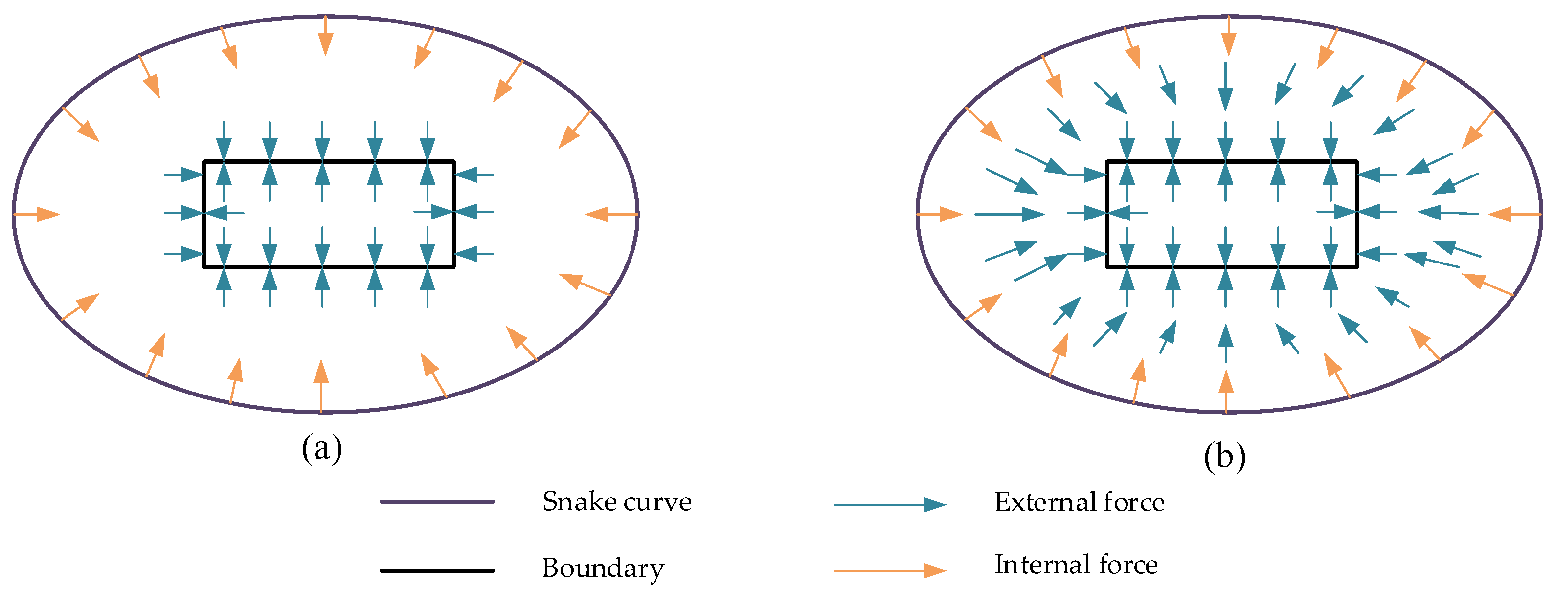
It can be seen from Equation (13) that when $\nabla f$ is small, ε is dominated by the first term. At this time, the coordinates $\left(x,y\right)$ are located far from the edge of the image, and V diffuses outward from the edge of the image, forming a smooth and slowly changing force field. When $\nabla f$ is large, the second term of ε plays a leading role. Obviously, when $\mathrm{V} = \nabla \mathrm{f}$, ε takes a minimum value. This function ensures that at the edge of the image, V is approximately equal to the gradient of the edge image. As shown in Figure 2a, the traditional Snake model takes the image gradient as the external force, which only acts on the adjacent region of the image boundary, while GVF can achieve the effect shown in Figure 2b, resulting in a slowly varying vector field in the homogeneous region of the image.

2.5. Point Cloud Back-Projection

We used the Snake algorithm to calculate the closed curve of the edge of the tree in the projection image of the tree. The closed curve is formed by connecting the corresponding pixel points in the image. Section 2.2 shows that each pixel of the tree in the gray image corresponds to a point set block that has a cross-section of $C_y\times C_z$ in the point clouds. We queried the corresponding point set for the pixel points that constitute the Snake curve one by one, and the combination of all the point sets is our final target result. The pixel matching process is shown in Algorithm 1.

Algorithm 1: Point Cloud Back-Projection Using Pixel Matching

Input: Data are the matrix of N rows and 3 columns composed of point cloud coordinates, where each    row represents the coordinates of a point and N is the number of point clouds;    Loc is the matrix of N rows and 2 columns formed by the corresponding pixel positions after    point cloud projection, where each row represents the projection position of a point, the row    number corresponds to Data, and N is the number of point clouds.    Snk is a matrix of M rows and 2 columns composed of the pixel positions corresponding to the    curve extracted by Snake, where M is the number of pixels.   k←1   for i = 1⋯M do    for j=1⋯N do     if Snk[i]==Loc[j] then      result[k]←Data[j]      K = k+1     end if    end for   end for   return result; Output: Matching results of point cloud contours;

3. Results and Discussion

3.1. Vegetation Classification

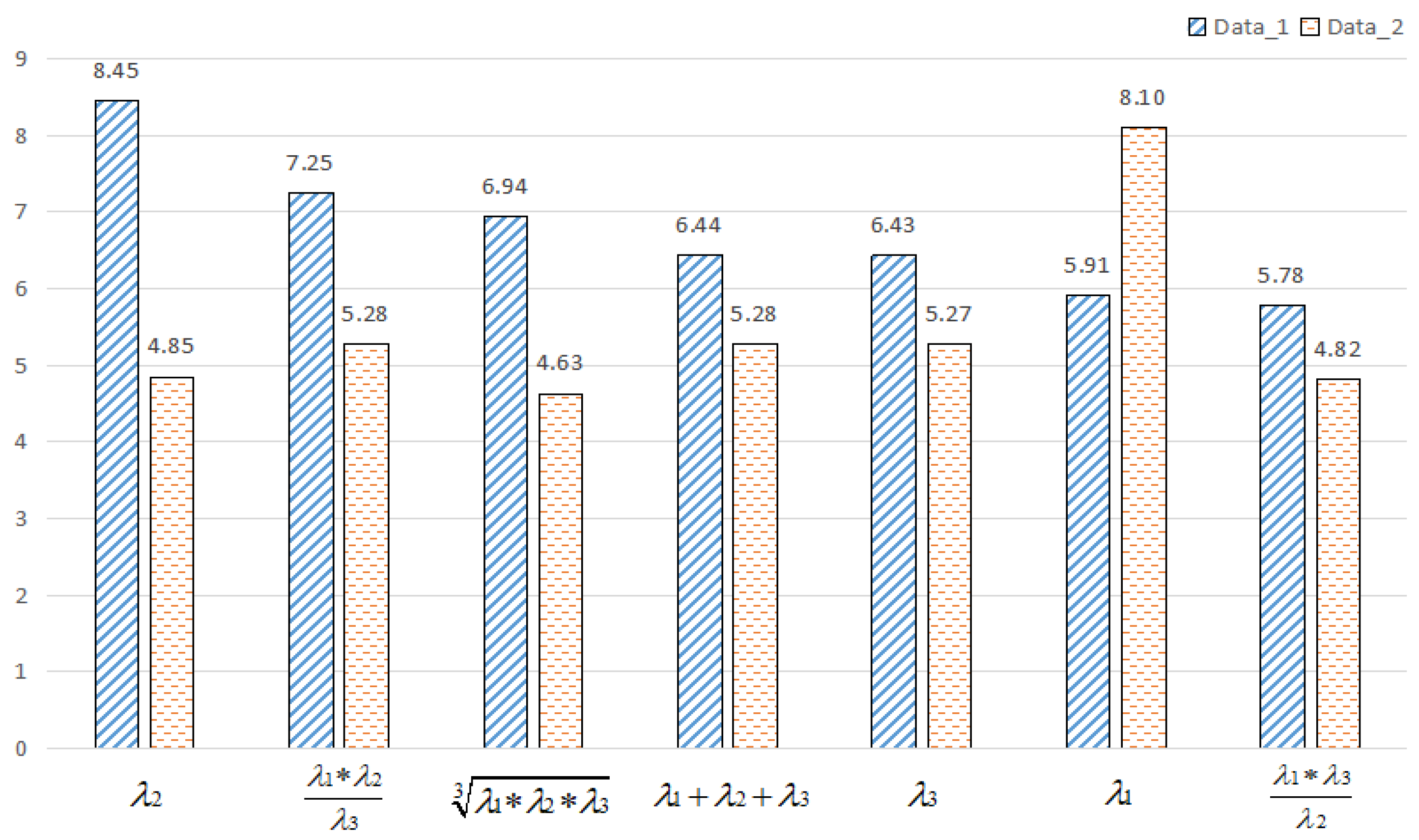
In order to segment the point cloud of the street tree, this study first classifies the point cloud data of the street tree scene. The purpose is to separate the tree part of the street scene, avoiding the problem of subsequent wrong segmentation and merging segmentation caused by weeds, shrubs, and uneven surface in the study area. We used each point and its three neighboring points (the number of neighboring points is chosen with respect to the point cloud density) to calculate the covariance matrix of each point and the corresponding eigenvalues and eigenvectors of this matrix, and then combine the eigenvalues and eigenvectors to form different features. In order to avoid redundant features affecting the classification accuracy, the Fisher feature selection algorithm was considered to calculate the weight of each feature. The top 95% of the features and their weight values are shown in Figure 3. Finally, we selected the top 95% features with large weights $\lambda 1$, $\lambda 2$, $\lambda 3$, Sum (${{\displaystyle \sum }}_{\lambda }$), Omnivariance ($O_{\lambda }$), Area ($J_{\lambda }$), and Pointing ($Z_{\lambda }$) as the input of SVM classifier, and the results show that the recall is 97.79%, precision is 99.93%, and the f1-score is 98.85%.

3.2. Projection and Contour Extraction

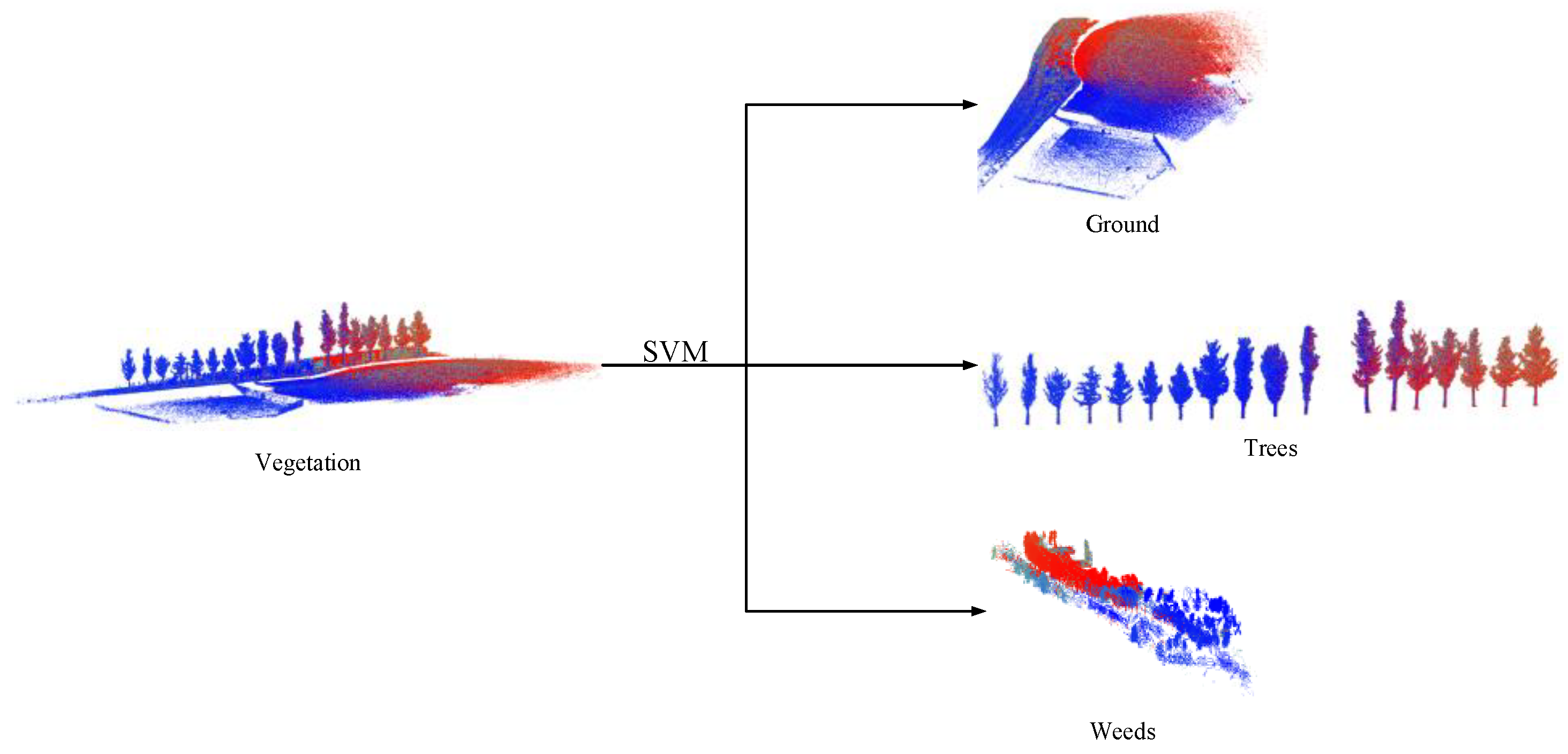
As shown in Figure 4, we classified part of the test road point clouds into three parts: trees, ground, and weeds. The main object of this study is the street tree point cloud data, so the tree point cloud is selected for 3D to 2D projection. In order to obtain the best projection surface, we projected different directions of the point cloud data every 30° interval and selected out the projection surface with the least overlap of pixels between the individual tree images as the target image of our segmentation. Figure 5 is the projection images of some randomly selected tree point clouds at different angles. As shown in Figure 5b, we chose the projection with the least overlap as our next research object.

If there is no overlap between the trees after projection, the individual tree can be directly obtained by back-projecting the image of each tree. However, after the optimal plane projection, some trees will still overlap. For this reason, the contours of trees are extracted in this method. The contour extraction can not only avoid the wrong segmentation caused by tree overlap, but can also effectively improve the efficiency of obtaining tree structure parameters.

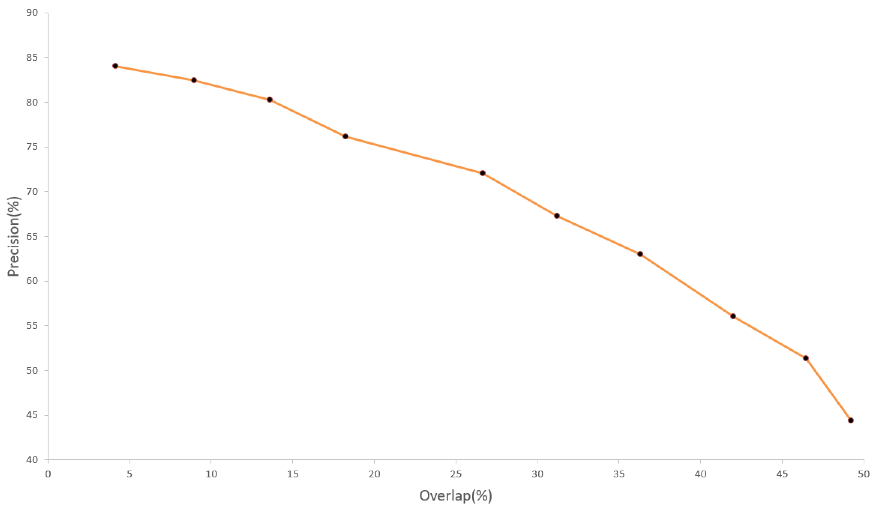
In addition, Figure 6 shows the relationship between the precision of the proposed method for individual tree segmentation and the overlap of a randomly selected tree, where the precision is defined as Equation (15) in Section 3.3 and the overlap of a tree is the ratio of the number of coincident pixels to the total number of pixels of the tree. It can be seen from the chart that, with the increase of overlap, the precision of individual tree segmentation is generally declining, but 95% of the street trees after the best plane projection have an overlap of less than 20%, so good segmentation results can be achieved.

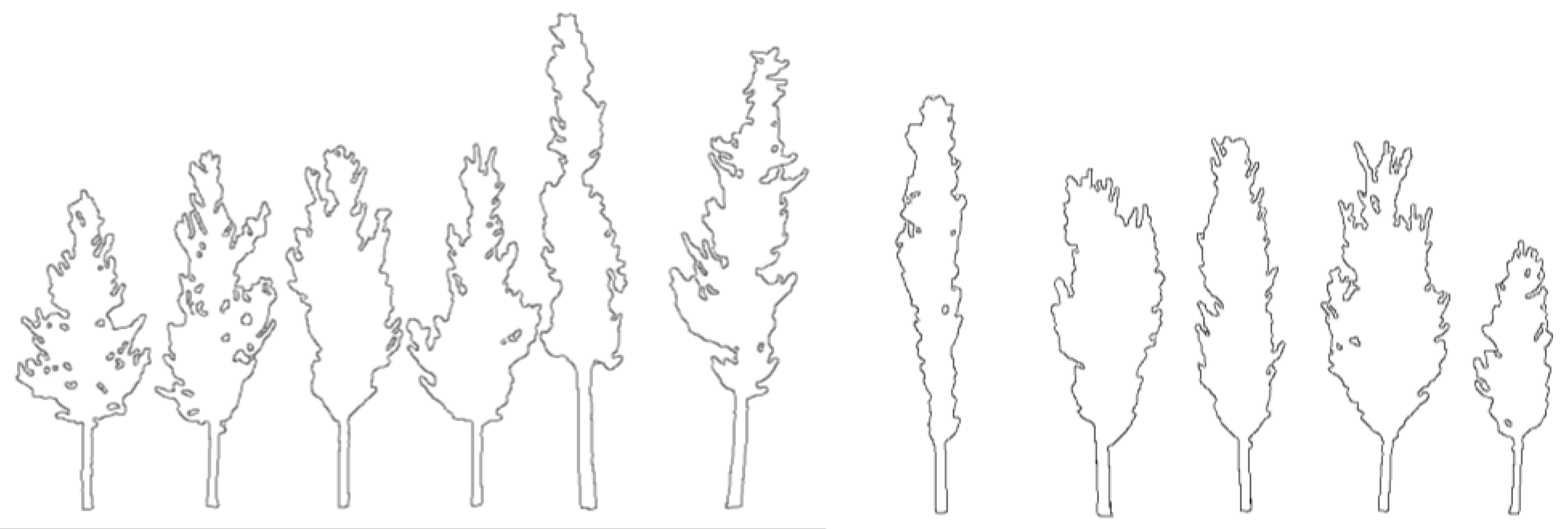
In order to extract the boundary of a tree, we first used the Canny algorithm to preliminarily calculate the edge points of the projection image. Although the Canny algorithm can extract the edge of the image more completely, there are still some problems. Using Gaussian filter to smooth the image will cause the edges to be unclear, so that some edges cannot be accurately identified. The different selection of double thresholds also affects the effect of edge detection. If the high threshold T_h is set as small, some weak edges can be easily detected, but we do not want to get the weak edges that are not outer contours. If the high threshold T_h is set as too large, the outer edge may break, resulting in the failure to obtain a continuous outer contour. Similarly, a too large or too small set of low threshold T_l can cause edge breakage or false edge, respectively. After several parameter adjustments and comparison of the resulting image, we selected the resulting images with broken outer edges and fewer non-target edges. At this time, the standard deviation of the Gaussian filter σ is 2, the high threshold T_h is set to 0.7, and the low threshold T_l = T_h × 0.4. The results calculated by some sample plots are shown in Figure 7.

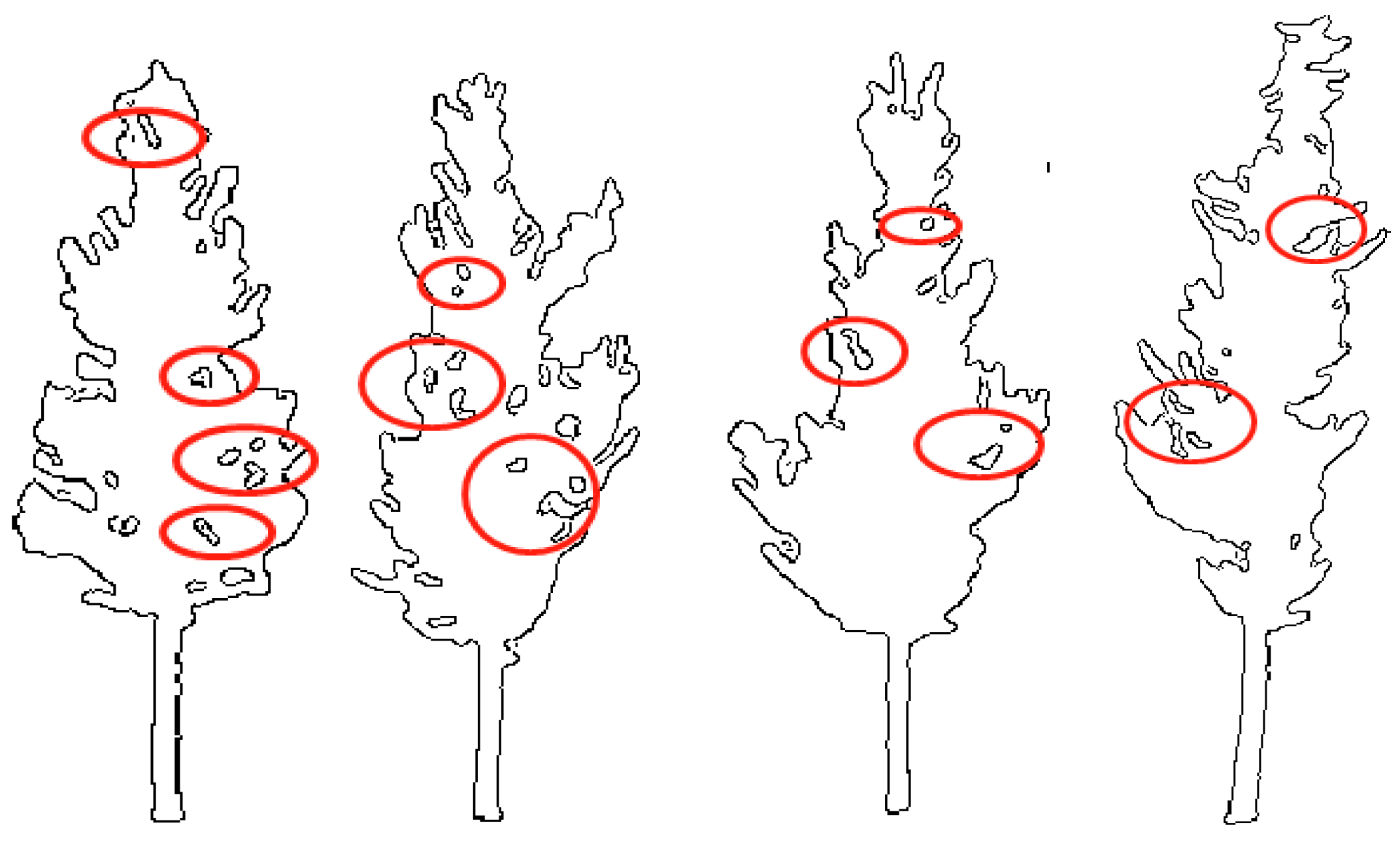
After the edge detection of vegetation projection image by Canny algorithm is realized, since the algorithm needs to be manually adjusted when performing double threshold processing, the adaptive ability is poor, and the edge is prone to discontinuity. Moreover, due to the partial gaps in the tree projection image, it is easy to produce false edges and affect the segmentation accuracy. As shown in Figure 8, after adjusting the high threshold, low threshold, and the standard deviation of the Gaussian filter, although the outer edges extracted from 80% of the individual tree grayscale images are relatively accurate, it is inevitable that some trees have a large proportion of false edges due to the large area and number of gaps.

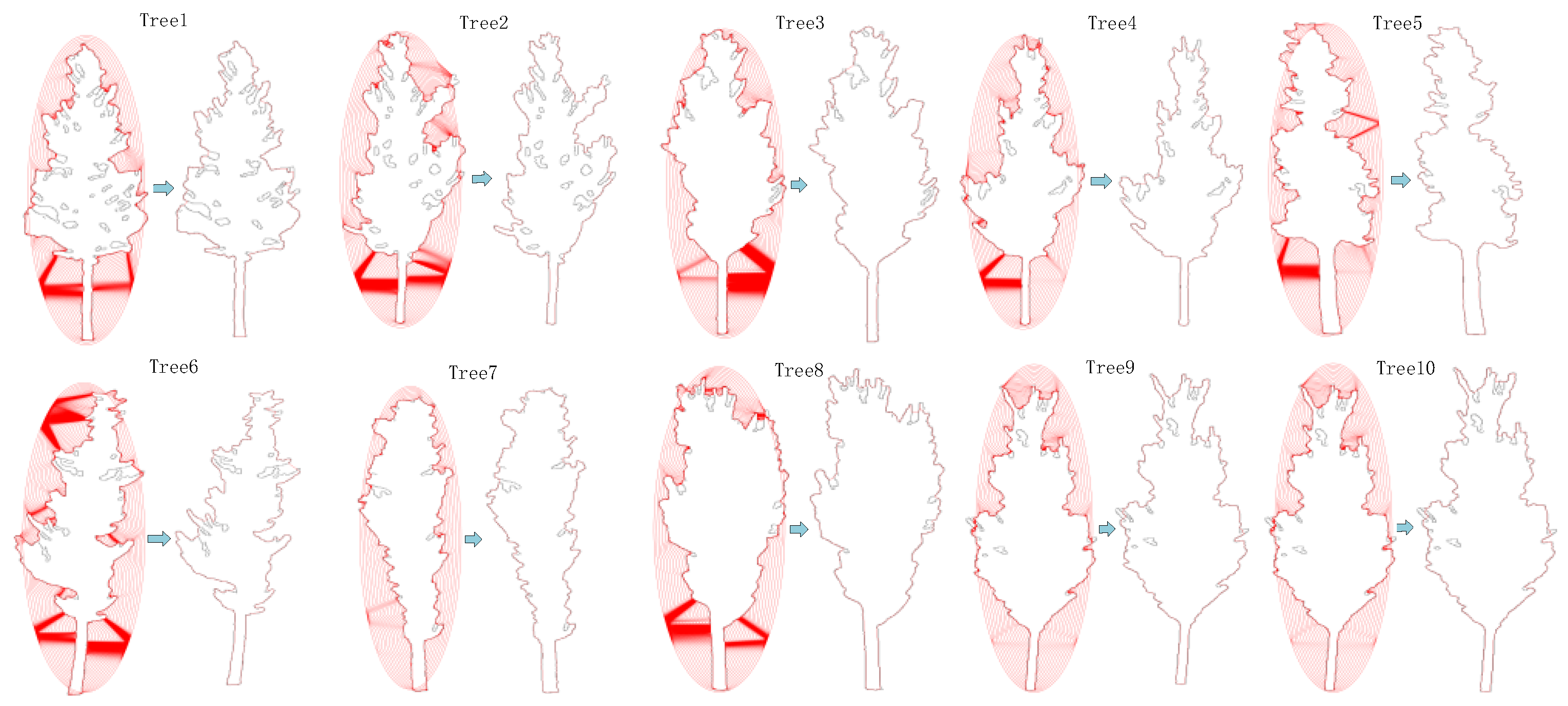
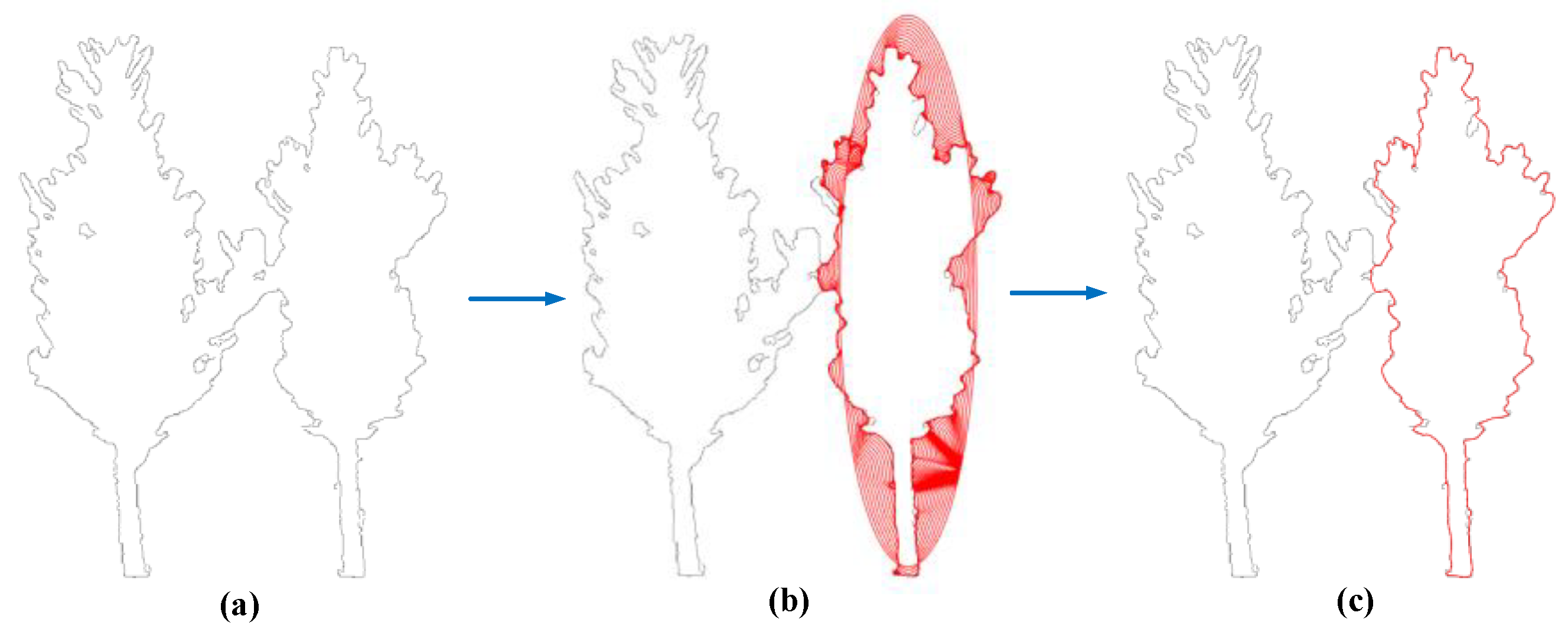
Active contour model (Snake) completes image segmentation through deformable and closed curve converging to target the edges, which can effectively extract tree contour and avoid the influence of ‘false edge’ and broken edge on experimental accuracy. On the basis of the result graph calculated by the Canny algorithm, we used the Snake model to extract the edge. As shown in Figure 9, the changing course of snake curve on a randomly selected tree is given. There are 169 trees in our study area, and the growth status and morphology of the trees are different. Figure 10 shows the iterative process and corresponding results of 10 randomly selected trees in the experimental plot, where the red is the Snake curve. As shown in Figure 11a, two trees overlap after projection, and the Canny algorithm cannot correctly segment the individual tree from the two trees. For this reason, we used the Snake algorithm to extract the individual tree. Figure 11b is the iterative process of Snake algorithm to extract the edge, and the red curve in Figure 11c is the extracted edge of the individual tree. Obviously, the edge calculated by Snake can effectively avoid the influence of false edge and accurately extract the outer edge of an individual tree.

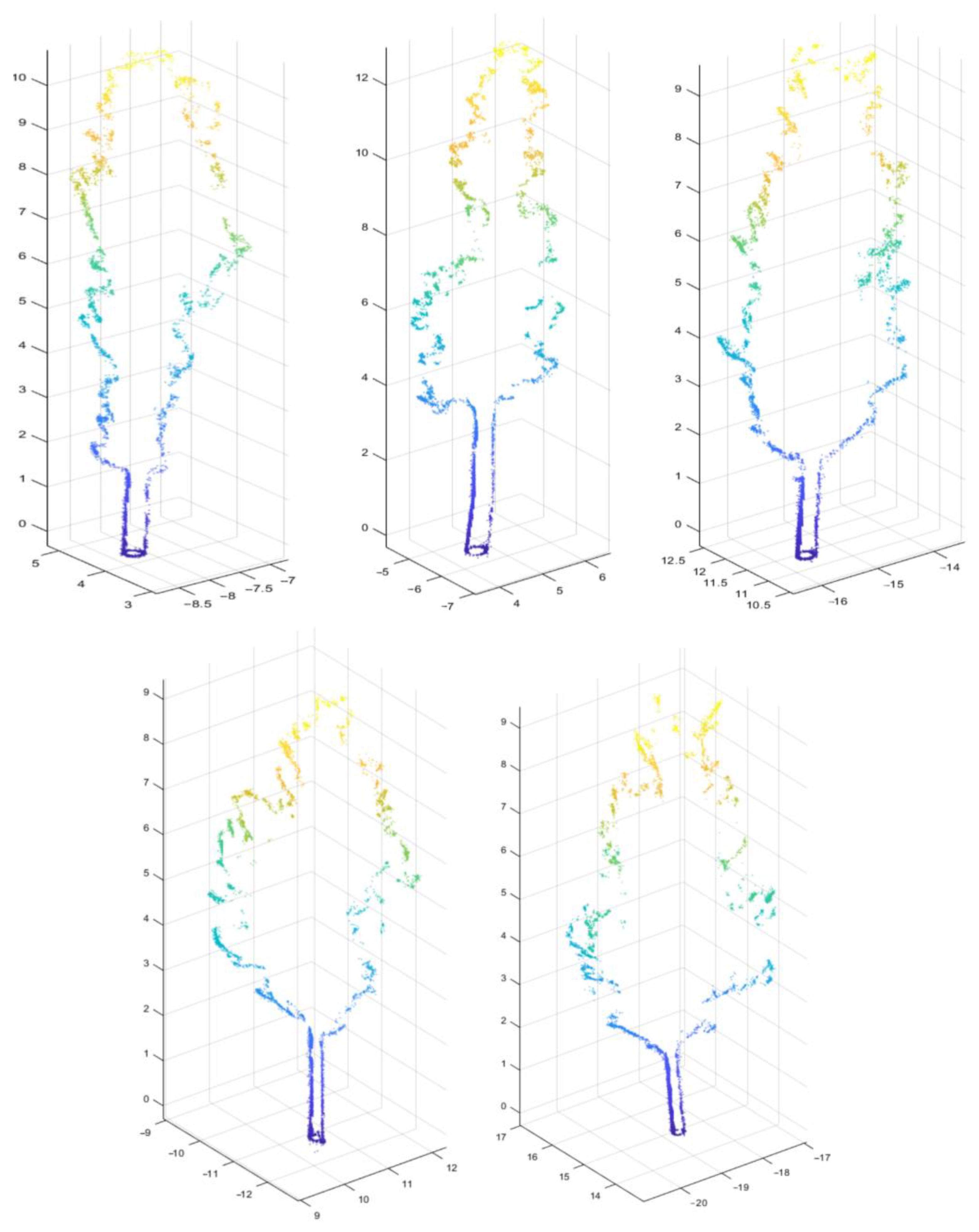
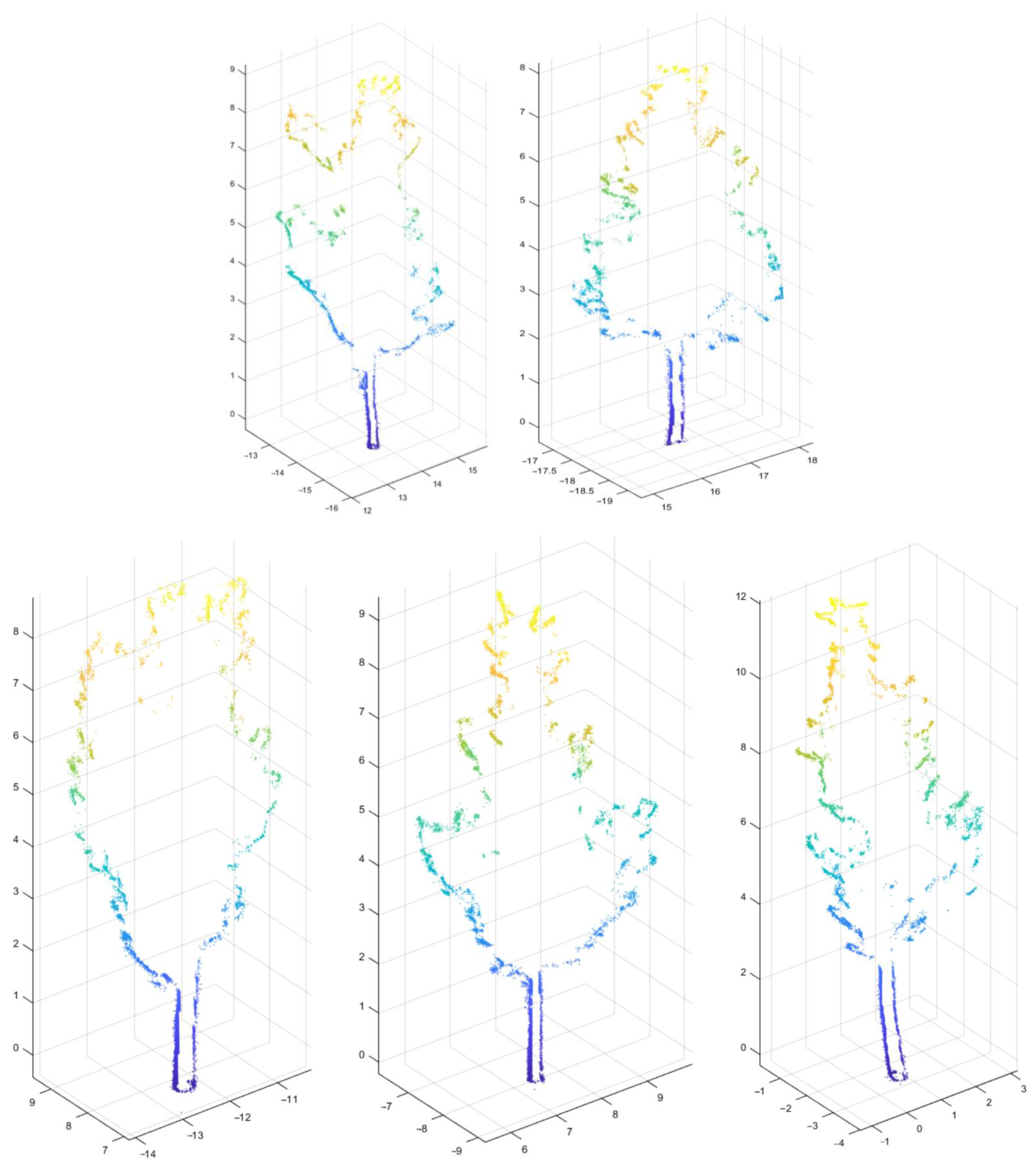
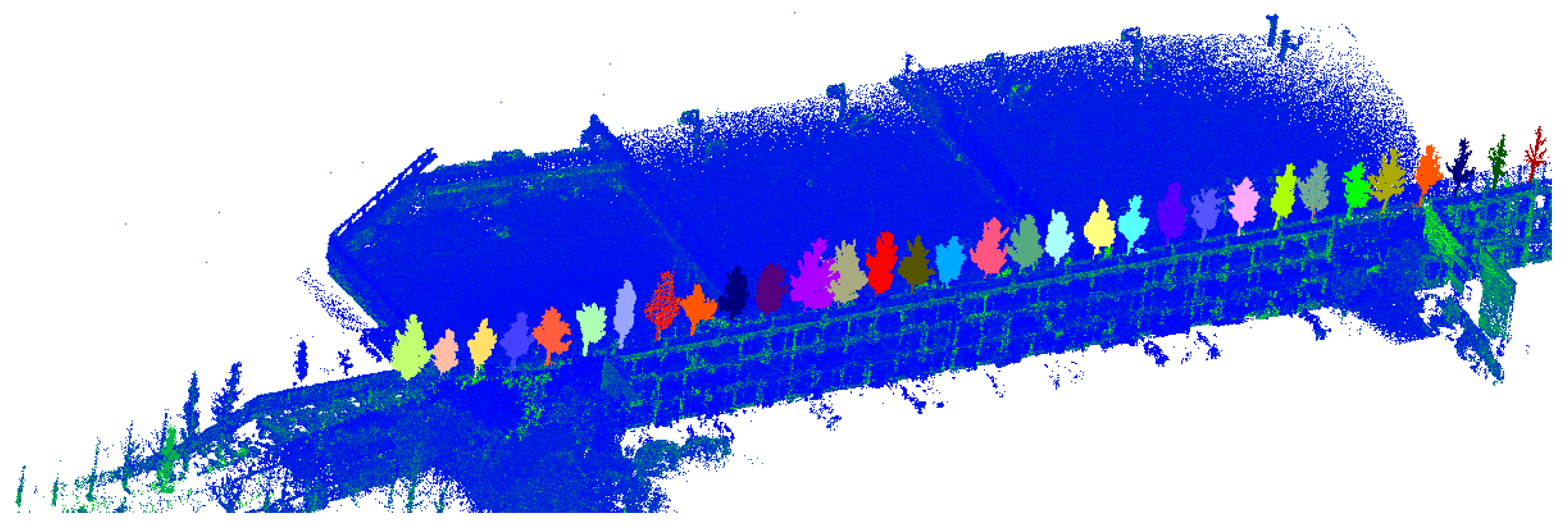
Finally, we used back-projection to match the pixels of Snake’s convergent curve position with the 3D point cloud to obtain the point cloud contour of a tree. The results of back-projection of 10 trees are shown in Figure 12 and Figure 13, showing the segmentation result in one scene.

3.3. Validation Approach

In order to evaluate the accuracy of tree point cloud segmentation, we manually segmented the outer edges of each tree, and then compared them with the results obtained by the proposed method. Quantitative evaluation includes three indicators: p (precision), r (recall), and q (quality). The corresponding calculation methods are:

$$\{\begin{array}{c}p=TP/\left(TP+FP\right)\\ r=TP/\left(TP+FN\right)\\ q=TP/\left(TP+FP+FN\right)\end{array}$$

(15)

TP represents the number of points belonging to the edge of the tree that are classified as the edge of the tree, that is, the points that are correctly classified. FP represents the number of points belonging to non-tree edges that are classified as tree edges, that is, the points that are misclassified. FN denotes the number of points that belong to edge points but are classified as non-edge points, that is, the points that are missed when classifying.

3.4. Evaluation and Analysis

The individual tree point cloud contour extracted by Snake is basically consistent with the real contour, which can achieve our target effect. In order to verify the effectiveness and necessity of combining Canny algorithm with Snake model, we compared the results extracted by the Canny algorithm with the results obtained by convergence of the Snake curve and calculated the performance indexes of point cloud individual tree segmentation, respectively.

Table 2. Segmentation precisions of 10 trees randomly selected from the experimental plot.

Method	Canny			Canny + Snake
Accuracy Metrics	p %	r %	q %	p %	r %	q %
Tree 1	82.86	80.57	69.06	86.90	79.85	71.27
Tree 2	81.71	78.48	66.76	86.58	88.62	77.92
Tree 3	86.65	81.75	72.60	87.57	88.73	78.80
Tree 4	85.82	79.65	70.39	88.48	83.98	75.70
Tree 5	91.83	93.00	85.89	91.90	93.96	86.77
Tree 6	87.08	88.67	78.36	85.89	83.58	73.49
Tree 7	90.52	89.06	81.46	91.51	89.16	82.35
Tree 8	89.54	88.95	80.57	89.40	83.16	75.70
Tree 9	92.41	75.80	71.36	91.55	89.64	82.79
Tree 10	90.83	81.97	75.70	91.01	89.11	81.90
…	…			…
All	90.28	81.38	74.83	91.67	85.33	79.19

shows the segmentation precisions of 10 randomly selected trees and the overall accuracy of the experimental data. It can be seen that the proposed method can accurately segment a tree, and the precision and recall are basically concentrated in 80–90%. When the Canny algorithm is used alone, precision, recall, and quality are 90.28%, 81.38%, and 74.83%, respectively. After combining Canny algorithm and Snake model, precision, recall, and quality are 91.67%, 85.33%, and 79.19%, respectively. Therefore, for most trees, the segmentation accuracy of the combined method of Canny and Snake is higher than that of using Canny algorithm alone, especially for trees with many gaps so that there are many “false edges” after processing by Canny algorithm, and the accuracy improvement is more obvious.

In the process of data preparation in Section 2.1, we performed Voxel-subsampling on the point clouds, which can not only reduce the data size but can also solve the problem of point cloud disorder, so that the point clouds are evenly distributed in space. Therefore, after the voxelization of point clouds, the segmentation precision based on the individual tree contour is actually equal to the segmentation precision before contour extraction.

We used the CHM-based watershed algorithm and the point cloud-based distance discriminant clustering algorithm to segment the individual tree of the experimental plot [26,27]. The idea of watershed algorithm is that after obtaining CHM, the gray value of the pixel is regarded as the canopy height, the local minimum is the tree vertex, and the affected area is the catchment area, that is, the canopy. The dam is constructed at the junction of the two catchment basins to form a watershed that distinguishes the canopy. The point cloud-based clustering algorithm uses the distance rule between trees, assuming that the highest point in the normalized point cloud data is the vertex of the tree, and then the distance iterative judgment is carried out from this point to realize the segmentation, where the distance threshold is set to the average crown radius of 1.81 m. After obtaining the segmented single tree, we also calculated the number of correctly classified points TP, misclassified points FP, and the points missed by classification FN through the ground truth of manual segmentation, and then get p, r, and q. The results are shown in

Table 3. Quantitative comparison between the proposed method and other methods.

Method	p %	r %	q %
Watershed algorithm	88.97	79.14	72.07
Point cloud-based cluster segmentation	91.86	83.18	77.47
Shadow-cut	91.67	85.33	79.19

. It can be seen that the segmentation effect of the proposed method in this paper is not inferior to that of the watershed algorithm and the point cloud-based clustering algorithm, mainly because of its superiority in handling side-view LiDAR vegetation point clouds.

Observing the experimental results of individual tree point cloud contour extraction, it can be seen that the main contour can be accurately extracted, but there are still some discontinuous broken edges. By observing the edge of the 2D image extracted by Snake and the point cloud contour after back-projection, it can be found that this is because the Snake curve cannot accurately reach some concave edges with narrow width or narrow entrance width after the convergence is completed, resulting in a small part of the concave region not being accurately extracted. For example, the positions A and B in Figure 14a are concave edges with a narrow entrance width and narrow width, respectively. From the convergence results of the Snake model shown in Figure 14b at these two positions, it can be seen that none of them converge completely on the narrow concave boundary. We observed and compared the vector field shown in Figure 14c,d. Figure 14c is the external force field of the narrow concave boundary, and Figure 14d is the external force field of the ordinary concave boundary. It can be seen that there are external forces perpendicular to the top of the U-shape in the X, Y, and Z positions of Figure 14d, which force the Snake curve to move to the concave boundary. Although the A position of Figure 14c has an external force pointing to the top of the U-shape, the curve tends to be stable due to the external force opposite to the top of the U-shape caused by the narrower entrance. The B position of Figure 14c is because the U-shape region is too narrow, resulting in only a small amount of external force parallel to the top of the U-shape, and no external force can promote the curve to move inward.

4. Conclusions

This study proposes an individual tree segmentation method for side-view LiDAR and implements individual tree segmentation for street tree point clouds. After the region of tree was classified, edge detection was performed on the projection of tree point clouds, and the individual tree can be segmented through the mapping relationship between the 2D image and the 3D point cloud. The conclusions are as follows:

(a)

Most of the current individual tree segmentation methods are realized by using the canopy information, thus ignoring the parameters at the lower part of the canopy. The proposed method takes full account of the complex structure and irregular density of vegetation point clouds and uses point cloud projection and back-projection to verify the practicability of edge detection method in 3D point cloud segmentation.

(b)

Moreover, in the processing of projection images, we combined Canny algorithm and Snake to effectively avoid the influence of false edges caused by tree gaps on the experimental results. The experiment shows that, for most trees, the results obtained by Snake are better than those obtained by Canny alone. For the sample plot, p, r, and q increased by 1.39%, 3.95%, and 4.36%, respectively.

(c)

The segmentation accuracy of this method can reach up to 91%, so the edge of a tree can be accurately extracted. However, due to the complex shape of some trees, the Snake curve does not converge completely for some narrow concave edges, resulting in some 3D point cloud contours to break, which is the main reason that affects the segmentation accuracy of the algorithm. In the subsequent research, improving the accuracy of individual tree segmentation will be one of our priorities, and we will study the extraction of tree skeletons through the separation of branches and leaves so as to better achieve 3D reconstruction of trees.

References

1. Han, X.; Sun, T.; Cao, T. Study on landscape quality assessment of urban forest parks: Take Nanjing Zijinshan National Forest Park as an example. Ecol. Indic. 2021, 120, 106902. [Google Scholar] [CrossRef]
2. Miao, C.; Yu, S.; Hu, Y.; Liu, M.; Yao, J.; Zhang, Y.; He, X.; Chen, W. Seasonal effects of street trees on particulate matter concentration in an urban street canyon. Sustain. Cities Soc. 2021, 73, 103095. [Google Scholar] [CrossRef]
3. Caneva, G.; Bartoli, F.; Zappitelli, I.; Savo, V. Street trees in Italian cities: Story, biodiversity and integration within the urban environment. Rend. Lincei. Sci. Fis. E Nat. 2020, 31, 411–417. [Google Scholar] [CrossRef]
4. Li, Q.; Yuan, P.; Liu, X.; Zhou, H. Street tree segmentation from mobile laser scanning data. Int. Ournal Remote Sens. 2020, 41, 7145–7162. [Google Scholar] [CrossRef]
5. Xu, S.; Han, W.; Ye, W.; Ye, Q. 3-D Contour Deformation for the Point Cloud Segmentation. IEEE Geosci. Remote Sens. Lett. 2021, 19, 1–5. [Google Scholar] [CrossRef]
6. Xia, S.; Chen, D.; Peethambaran, J.; Wang, P.; Xu, S. Point Cloud Inversion: A Novel Approach for the Localization of Trees in Forests from TLS Data. Remote Sens. 2021, 13, 338. [Google Scholar] [CrossRef]
7. Næsset, E.; Økland, T. Estimating tree height and tree crown properties using airborne scanning laser in a boreal nature reserve. Remote Sens. Environ. 2002, 79, 105–115. [Google Scholar] [CrossRef]
8. Xu, S.; Li, X.; Yun, J.; Xu, S. An Effectively Dynamic Path Optimization Approach for the Tree Skeleton Extraction from Portable Laser Scanning Point Clouds. Remote Sens. 2021, 14, 94. [Google Scholar] [CrossRef]
9. Xia, S.; Xu, S.; Wang, R.; Li, J.; Wang, G. Building Instance Mapping from ALS Point Clouds Aided by Polygonal Maps. IEEE Trans. Geosci. Remote Sens. 2021, 60, 1–13. [Google Scholar] [CrossRef]
10. Xu, S.S.; Xu, S. Identification of Street Trees’ Main Nonphotosynthetic Components from Mobile Laser Scanning Data. Opt. Mem. Neural Netw. 2020, 29, 305–316. [Google Scholar] [CrossRef]
11. Wulder, M.A.; White, J.C.; Stinson, G.; Hilker, T.; Kurz, W.A.; Coops, N.C.; St-Onge, B.; Trofymow, J.A. Implications of differing input data sources and approaches upon forest carbon stock estimation. Env. Monit Assess 2010, 166, 543–561. [Google Scholar] [CrossRef] [PubMed] [Green Version]
12. Chen, Q.; Baldocchi, D.; Gong, P.; Kelly, M. Isolating Individual Trees in a Savanna Woodland Using Small Footprint LIDAR Data. Photogramm. Eng. Remote Sens. 2006, 72, 923–932. [Google Scholar] [CrossRef] [Green Version]
13. Koch, B.; Heyder, U.; Weinacker, H. Detection of Individual Tree Crowns in Airborne Lidar Data. Photogramm. Eng. Remote Sens. 2006, 72, 357–363. [Google Scholar] [CrossRef] [Green Version]
14. Ayrey, E.; Fraver, S.; Kershaw, J.A., Jr.; Kenefic, L.S.; Hayes, D.; Weiskittel, A.R.; Roth, B.E. Layer Stacking: A Novel Algorithm for Individual Forest Tree Segmentation from LiDAR Point Clouds. Can. Ournal Remote Sens. 2017, 43, 16–27. [Google Scholar] [CrossRef]
15. Yunsheng, W.; Holger, W.; Barbara, K. A Lidar Point Cloud Based Procedure for Vertical Canopy Structure Analysis and 3D Single Tree Modelling in Forest. Sensors 2008, 8, 3938–3951. [Google Scholar]
16. Morsdorf, F.; Meier, E.; Kötz, B.; Itten, K.I.; Dobbertin, M.; Allgöwer, B. LIDAR-based geometric reconstruction of boreal type forest stands at single tree level for forest and wildland fire management. Remote Sens. Environ. 2004, 92, 353–362. [Google Scholar] [CrossRef]
17. Vega, C.; Hamrouni, A.; El Mokhtari, S.; Morel, J.; Bock, J.; Renaud, J.-P.; Bouvier, M.; Durrieu, S. PTrees: A point-based approach to forest tree extraction from lidar data. Int. Ournal Appl. Earth Obs. Geoinf. 2014, 33, 98–108. [Google Scholar] [CrossRef]
18. Xu, S.; Zhou, X.; Ye, W.; Ye, Q. Classification of 3D Point Clouds by a New Augmentation Convolutional Neural Network. IEEE Geosci. Remote Sens. Lett. 2022, 19, 1–5. [Google Scholar]
19. Lee, K.H.; Woo, H.; Suk, T. Data reduction methods for reverse engineering. Int. Ournal Adv. Manuf. Technol. 2001, 17, 735–743. [Google Scholar] [CrossRef]
20. Han, X.F.; Jin, J.S.; Wang, M.-J.; Jiang, W.; Gao, L.; Xiao, L. A review of algorithms for filtering the 3D point cloud. Signal Process. Image Commun. 2017, 57, 103–112. [Google Scholar] [CrossRef]
21. Lin, C.H.; Chen, Y.; Su, P.L.; Chen, C.H. Eigen-feature analysis of weighted covariance matrices for LiDAR point cloud classification. Isprs J. Photogramm. Remote Sens. 2014, 94, 70–79. [Google Scholar] [CrossRef]
22. Wang, D.; Hollaus, M.; Pfeifer, N. Feasibility of machine learning methods for separating wood and leaf points from terrestrial laser scanning data. ISPRS Ann. Photogramm. Remote Sens. Spat. Inf. Sci. 2017, IV-2/W4, 157–164. [Google Scholar] [CrossRef]
23. Guo, Y.F.; Shu, T.T.; Yang, Y.; Li, S.J. Feature Extraction Method Based on the Generalised Fisher Discriminant Criterion and Facial Recognition. Pattern Anal. Appl. 2001, 4, 61–66. [Google Scholar] [CrossRef]
24. Yue, J.; Fang, L.; Ghamisi, P.; Xie, W.; Li, J.; Chanussot, J.; Plaza, A.J. Optical Remote Sensing Image Understanding with Weak Supervision: Concepts, Methods, and Perspectives. IEEE Geosci. Remote Sens. Mag. 2022, 10, 250–269. [Google Scholar] [CrossRef]
25. Canny, J. A Computational Approach to Edge Detection. IEEE Trans. Pattern Anal. Mach. Intell. 1986, PAMI-8, 679–698. [Google Scholar] [CrossRef]
26. Mongus, D.; Žalik, B. An efficient approach to 3D single tree-crown delineation in LiDAR data. ISPRS J. Photogramm. Remote Sens. 2015, 108, 219–233. [Google Scholar] [CrossRef]
27. Reitberger, J.; Schnörr, C.; Krzystek, P.; Stilla, U. 3D segmentation of single trees exploiting full waveform LIDAR data. ISPRS J. Photogramm. Remote Sens. 2009, 64, 561–574. [Google Scholar] [CrossRef]
Figure 1. Flowchart of the proposed point cloud individual tree segmentation method.
Remotesensing 14 05742 g001
Figure 2. (a) Snake with image gradient as external force. (b) Snake with GVF as external force.
Remotesensing 14 05742 g002
Figure 3. Weight corresponding to each feature.
Remotesensing 14 05742 g003
Figure 4. Process of vegetation point cloud classification.
Remotesensing 14 05742 g004
Figure 5. Pixel coincidence (a) and non-coincidence (b) projection map.
Remotesensing 14 05742 g005
Figure 6. The relationship between the precision of the proposed method for individual tree segmentation and the overlap of a randomly selected tree.
Remotesensing 14 05742 g006
Figure 7. Tree edges extracted by Canny algorithm.
Remotesensing 14 05742 g007
Figure 8. Canny algorithm inevitably produces false edges as shown in the red circles.
Remotesensing 14 05742 g008
Figure 9. Changing course of snake curve on a randomly selected tree.
Remotesensing 14 05742 g009
Figure 10. Convergence processes and results of Snake curves.
Remotesensing 14 05742 g010
Figure 11. The process of individual tree segmentation when tree projections overlap. (a) Two trees overlap after projection, (b) the iterative process of Snake algorithm to extract the edge, (c) the red curve is the extracted edge of the individual tree.
Remotesensing 14 05742 g011
Figure 12. Segmentation precisions of 10 trees randomly selected from the experimental plot.
Remotesensing 14 05742 g012aRemotesensing 14 05742 g012b
Figure 13. The segmentation results in one scene.
Remotesensing 14 05742 g013
Figure 14. (a) Narrow concave boundary, (b) convergence results of narrow concave boundary, (c) external force field within the narrow boundary concavity, (d) external force field within an ordinary boundary concavity. The positions A and B are concave edges with a narrow entrance width and narrow width, respectively. X, Y, and Z are the positions where the external forces are perpendicular to the top of the U-shape.
Remotesensing 14 05742 g014