Article

Analyzing the Spatially Heterogeneous Relationships between Nighttime Light Intensity and Human Activities across Chongqing, China

1
Key Laboratory of Spatial Data Mining and Information Sharing of Ministry of Education, National & Local Joint Engineering Research Center of Satellite Geospatial Information Technology, Fuzhou University, Fuzhou 350108, China
2
The Academy of Digital China, Fuzhou University, Fuzhou 350108, China
3
Key Laboratory of Geographic Information Science (Ministry of Education), East China Normal University, Shanghai 200241, China
4
School of Geographic Sciences, East China Normal University, Shanghai 200241, China
*
Author to whom correspondence should be addressed.
Remote Sens. 2022, 14(22), 5695; https://doi.org/10.3390/rs14225695
Submission received: 6 October 2022 / Revised: 5 November 2022 / Accepted: 9 November 2022 / Published: 11 November 2022

Abstract

:
Nighttime light (NTL) intensity is highly associated with the unique footprint of human activities, reflecting the development of socioeconomic and urbanization. Therefore, better understanding of the relationship between NTL intensity and human activities can help extend the applications of NTL remote sensing data. Different from the global effect of human activities on NTL intensity discussed in previous studies, we focused more attention to the local effect caused by the spatial heterogeneity of human activities with the support of the multiscale geographically weighted regression (MGWR) model in this study. In particular, the Suomi National Polar Orbiting Partnership/Visible Infrared Imaging Radiometer Suite (NPP/VIIRS) NTL data within Chongqing, China were taken as example, and the point of interest (POI) data and road network data were adopted to characterize the intensity of human activity type. Our results show that there is significant spatial variation in the effect of human activities to the NTL intensity, since the accuracy of fitted MGWR (adj.R2: 0.86 and 0.87 in 2018 and 2020, respectively; AICc: 4844.63 and 4623.27 in 2018 and 2020, respectively) is better than that of both the traditional ordinary least squares (OLS) model and the geographically weighted regression (GWR) model. Moreover, we found that almost all human activity features show strong spatial heterogeneity and their contribution to NTL intensity varies widely across different regions. For instance, the contribution of road network density is more homogeneous, while residential areas have an obviously heterogeneous distribution which is associated with house vacancy. In addition, the contributions of the commercial event and business also have a significant spatial heterogeneity distribution, but show a distinct decrement when facing the COVID-19 pandemic. Our study successfully explores the relationship between NTL intensity and human activity features considering the spatial heterogeneity, which aims to provide further insights into the future applications of NTL data.

1. Introduction

Due to rapid socioeconomic development, artificial nighttime lights gradually alter the spatial distribution of brightness on the Earth’s surface at night [1]. Nighttime light (NTL) remote sensing images provide a direct signature of human activity [2], different from traditional daytime remote sensing data which primarily monitor the surface environment information. The two commonly used NTL data are the Defense Meteorological Satellite Program/Operational Linescan System (DMSP/OLS) NTL data and Suomi National Polar-orbiting Partnership-Visible Infrared Imaging Radiometer Suite (NPP/VIIRS) NTL data. Some studies have demonstrated that there are statistically significant correlations between NTL intensity and human activities at the different scales [3,4,5,6,7]. Therefore, the DMSP/OLS and NPP/VIIRS NTL data are generally associated with socioeconomic topics [8], including gross domestic product [3,9,10], extracting urban built-up area [11,12], estimating population [13,14,15,16], house vacancy [17], poverty [18,19], urbanization [20], and electricity consumption [21,22,23]. Recently, NTL data are also used in the perspective of environmental fields, such as carbon dioxide emissions [24], light pollution [25,26], human health [27,28], and food security [29]. Compared with the DMSP/OLS NTL data, the NPP/VIIRS data have significant improvement in spatial resolution and radiometric detection range [30]. Thus, VIIRS data might specifically be used to characterize the human activity information from cities, towns, and other places.
Most previous studies have demonstrated that NTL intensity is globally correlated with human activities by using classical statistical methods and machine learning models. For instance, Li, et al. [31] used an unmixing model to quantify the land use contribution to DMSP/OLS and NPP/VIIRS NTL intensity in Berlin and Massachusetts. Ma [32] used the LULC and POIs data to analyze the relationship between NPP/VIIRS NTL intensity and land features (e.g., Cropland, water, urban land, built-up land, etc.) at pixel level. Levin and Zhang [7] found that road network density shows a significant correlation with NTL intensity in densely populated areas using general linear models (GLMs). Chen, et al. [33] quantified the contribution of various POI categories to DMSP/OLS NTL intensity using the ordinary least squares (OLS) regression, and the results showed that shopping centers and companies were the main contributors to NTL intensity. Wang, et al. [34] used the LULC and POIs data to construct different artificial surface features at the parcel level and used random forest (RF) regression models to explore the contribution of each feature to NTL intensity. The spatial distribution for NTL intensity was uneven due to the inherent spatial heterogeneity within geographical phenomena including multiple socioeconomic factors [35]. Nevertheless, the abovementioned relationships between human activity and NTL intensity are global and non-spatial, with limited consideration of the local differences and spatial heterogeneity of human activity.
To fill this gap, the geographically weighted regression (GWR) model was proposed by Brunsdon, et al. [36] to measure the variation trend of factors in space. Based on the spatial non-stationary characteristics, the GWR model effectively addresses the spatial heterogeneity that is ignored by the traditional regression models in performing regression analysis [37]. In practical research, Ye, et al. [38] used the GWR model to downscale NPP/VIIRS images based on multi-source spatial data. However, GWR assumed that all variables have the same spatial heterogeneity, and thus does not allow each variable to have their own bandwidth [39]. In many cases, including human activity, this assumption is not valid because the human activity features can be different with varying spatial scales.
Owing to the advantage of the multiscale geographically weighted regression (MGWR) model, the effects of each variable can be distinguished from global and local perspectives by allowing variables to be varied over space and at different scales [40,41,42,43] Generally, MGWR has been successfully used to analyze socioeconomic topics such as urban heat island [44], obesity [45], and public health crises [41,46]. So far, there is no literature adopting this model to analyze the local effects of human activity on NTL intensity. To extend the applications of NTL remote sensing images, it is crucial to explore the relationship between the NPP/VIIRS NTL intensity and human activities while considering spatial heterogeneity.
In this study, POIs and road network data were selected to measure human activity features, and the MGWR model was used to analyze the relationship between various human activity features and NTL intensity in the central urban area of Chongqing. The main objectives of this study are: (1) to measure the contribution of each human activity feature to the NPP/VIIRS NTL intensity in 2018 and 2020, and (2) to identify and analyze the spatial pattern of feature contributions, as well as the drivers behind the change in feature contributions.

2. Study Area and Dataset

2.1. Study Area

The urban area from nine core administrative districts within Chongqing, China was selected as our study area based on the following two reasons: First, Chongqing, located in the upper reaches of the Yangtze River, is one of the four municipalities in China and has had rapid economic development and population growth since 1997, especially within the nine districts. Meanwhile, Chongqing has a complex topography with more than 70% area of mountainous, resulting in a complex distribution of human activities [47,48]. Based on this background, this area is suitable for exploring the relationship between NTL intensity and human activities while considering spatial heterogeneity. Second, the nighttime light intensity is mainly from the urban area, we hence used global urban boundaries (GUBs) data to filter out non-urban areas, as shown in Figure 1.

2.2. Data Sources and Preprocessing

The dependent variable (NTL intensity) and the independent variables (human activity features) defined in this study are composed of overlying eight maps, including NPP/VIIRS NTL data (Figure 2a), POIs (6 categories, Figure 2b–g), and road network (Figure 2c). Figure 2 shows the spatial distribution of NTL intensity, POIs, and road network in 2018. Moreover, the GUB data were used to delineate the urban area in Chongqing. Since all variables we calculated in this study required the area of each grid, all these spatial data were projected to the Albers Equal Area Conic Projection for the convenience of the subsequent study.

2.2.1. VIIRS Data

In this study, the annual average global NPP/VIIRS NTL data (version 2) in 2018 and 2020 were adopted to provide NTL intensity, which are generated by the Earth Observation Group (EOG) and can be accessed from https://payneinstitute.mines.edu/eog/nighttime-lights/ (accessed on 18 May 2021). The data have been stripped of irrelevant features such as biomass burning, aurora, and background [49], and its spatial resolution is 15 arc second (approximately 500 m) with the unit of nW cm−2 sr−1. We resampled the projected NPP/VIIRS NTL data to generate raster grids with a spatial resolution of 500 m (Figure 2a).

2.2.2. POI Data

The POI data were collected from Amap (https://lbs.amap.com/ (accessed on 5 May 2021)) to reflect the intensity of each human activity type. The original POI data consist of 23 major categories (such as finance and insurance services, enterprises, shopping, transportation service, etc.). Based on our research purpose, we reclassified the POI data into six categories (Table 1) according to the criteria of Gong, et al. [50]. Totally, 152,437 and 155,454 POI records were selected for the years of 2018 and 2020, respectively. Figure 2b–g shows that POI data cover most pixels with NTL intensity. Due to the lack of a long time series of POI data, we must analyze the contribution from 2018 to 2020.

2.2.3. OpenStreetMap Data

The road network data from OpenStreetMap (http://www.openstreetmap.org (accessed on 12 June 2021)) was selected to reflect the road network density, since streetlights and traffic lights are the main sources of NTL in urban areas [51,52]. Figure 2c illustrates the road network adopted by Chongqing, including motorway, trunk road, primary road, secondary road, and tertiary road, covering most areas of the city.

2.2.4. GUB Data

The global urban boundaries (GUBs) data can be obtained from http://data.ess.tsinghua.edu.cn/ (accessed on 2 June 2021). Compared with the NTL and Landsat images derived results [53,54], GUB data can show more details about urban fringe areas [55]. Due to the lack of long-term data, we used GUB data for 2018 to delineate urban areas. The final study area was obtained by clipping the projected NTL data according to GUB, and a total of 4321 grids with 500 m resolution grids were finally determined.

3. Methods

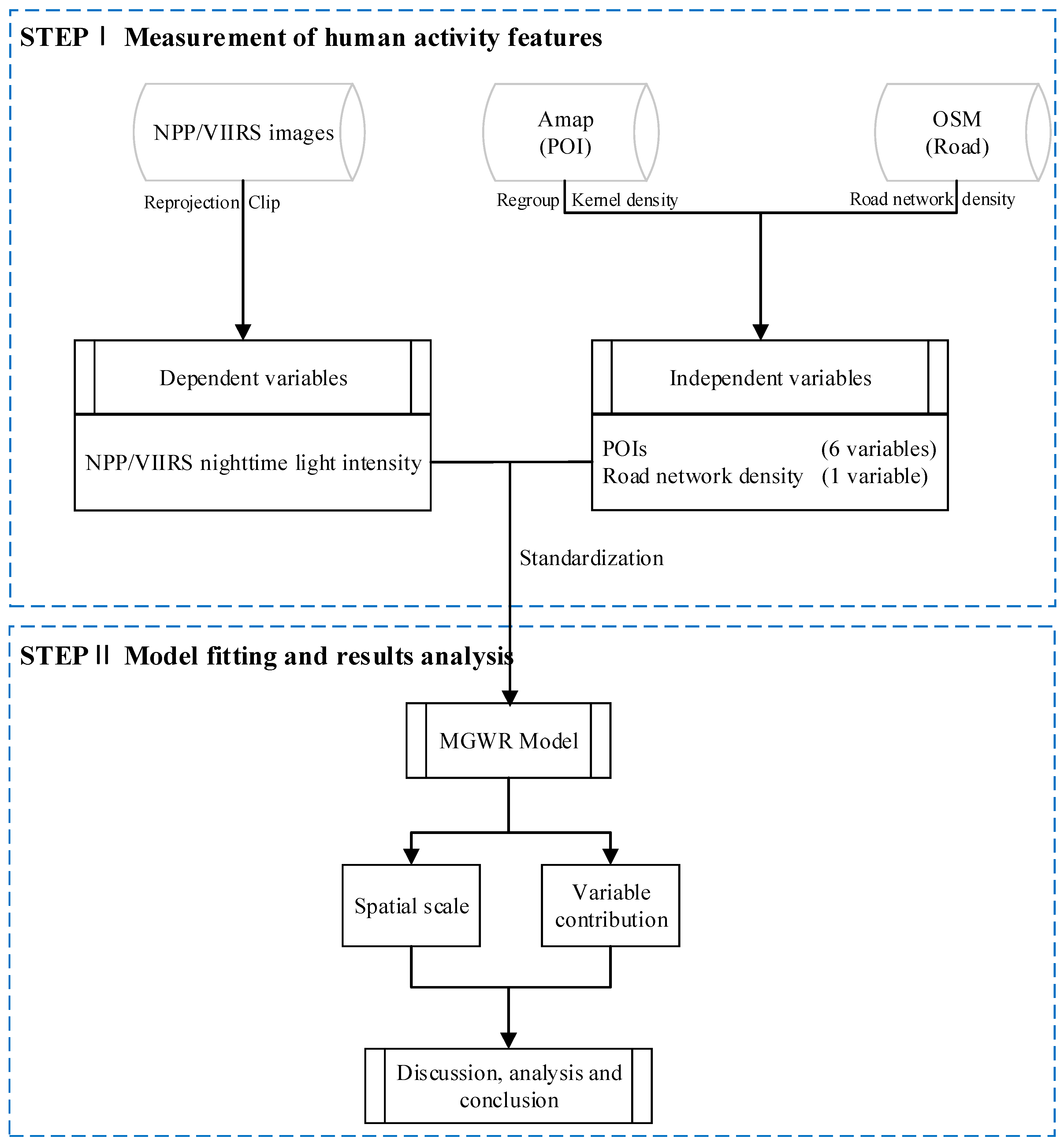
The framework of the study mainly consists of two steps (Figure 3): (I) Measurement of human activity features. The POI data and road network data were adopted to construct 7 variables at pixel level to refer human activity features by calculating their density; (II) and model fitting and results analysis. All the variables were input into the MGWR model to explore the local relationship between human activities and NPP/VIIRS NTL intensity, as well as their spatial scale variation.

3.1. Measurement of Human Activity Features

The 7 human activity features adopted in this study contain two parts: The first 6 features are from the 6 categories of POI data by using kernel density estimation (KDE), and the last feature is from the road network data by calculating the ratio between the total length of the road network and pixel area. To facilitate comparing the contribution of each variable to NPP/VIIRS NTL intensity and bandwidths obtained from the MGWR mode [56], all the independent variables and NTL intensity were standardized to the same range by Equation (1):
X k = X k 0 μ k 0 σ k 0
where Xk is the standardized value for the kth variable; Xk0 is the original value of the kth variable; μk0 is the mean value for Xk0; and σk0 is the standard deviation for Xk0.

3.1.1. Human Activity Features from POI Data

The kernel density estimation (KDE) of each POI class was conducted to weaken the influence caused by the lack of area characteristic in POI data. The KDE can visualize the spatial variation characteristics of the point element density, which is widely used in the geological regional analysis [57]. The calculation of the kernel density estimate is as follows:
f ( x ) = i = 1 n 1 h 2 k ( x x i h )
where f(x) is the estimated kernel density value at location x; k is the kernel function; xxi is the distance between POIs location xi and x; h is the radius; and n is the total number of POIs contained within radius h.
In this study, the 6 categories of POIs data, as mentioned in Table 1, were separately input into the KDE model with a radius of 1500 m to obtain the 6 human activity features. Particularly, these features include transportation index (TI), residential index (RI), administrative index (AI), sports and cultural index (SCI), business office index (BOI), and commercial service index (CSI).

3.1.2. Human Activity Feature from Road Network

The road network density (RND) reflects the development level of urban roads and can be calculated by the following Equation (3):
RND i = L i A i
where Li is the total road network length in the ith pixel; and Ai is the area of ith pixel.

3.2. Regression Models

To comprehensively analyze the relationship between NTL intensity and human activities, three models are used in this study. One is a traditional global model, named the ordinary least squares (OLS) regression model, and the other two models are geographically weighted regression (GWR) and multiscale geographically weighted regression (MGWR), which are local models.

3.2.1. OLS Regression Model

The OLS has been commonly used in non-spatial linear regression analysis to describe the correlation of a dependent variable with some independent variables. The OLS is denoted by:
y i = β 0 + i = 1 n X i β i + ε i
where yi is the dependent variable, representing the NTL intensity of the ith pixel; β0 is the intercept of the model; Xi corresponds to the ith explanatory variable of the model (i = 1 to n); βi is the regression coefficients, which reflects the contribution of each variable to the NTL intensity; and εi indicates the random error item.

3.2.2. GWR and MGWR Models

Geographically weighted regression (GWR) is a kind of regression method that can effectively address and explain the local variation of features, bringing the geospatial variation in selected features into consideration [36,58]. The GWR model is shown in Equation (5):
y i = β 0 ( u i , v i ) + j = 1 n β j ( u i , v i ) X i j + ε i
where (ui, vi) is the spatial coordinate of pixel i; β0 is the intercept; βj is the coefficient of the variable j of pixel i; Xij denotes jth variable of pixel i; and εi is a random error item. Parameter estimates for each independent variable and at each pixel in matrix form is denoted by [59]:
β ^ ( i ) = ( X T W ( i ) X ) 1 X T W ( i ) Y
where β ^ ( i ) is the vector of parameter estimates (t × 1), X indicates the matrix of independent variable (n × t), W(i) is the spatial weights matrix (n × n), and Y is a t × 1 vector of observations of the dependent variable. W(i) is constructed from the weights of each pixel based on its distance from location i. To calculate the matrix W(i), the kernel function and bandwidth should be specified. The Gaussian and bi-square kernel function are commonly used to implement, and the bandwidth is determined based on Euclidean distance or the number of nearest neighbors [41,45,46].
The GWR can capture the spatially non-stationarity of variables, which is a significant improvement over global regression (such as OLS), whereas it assumes that the scale of all variables is constant in space. Based on this limitation, Fotheringham, Yang, and Kang [39] developed the MGWR model, which allows variables to use different bandwidths and can better reflect the spatial variation process of variables and NTL intensity. Moreover, the model can avoid introducing too much noise and bias to improve the model fitting performance. It can be calculated by Equation (7):
y i = j = 1 k β b w j ( u i , v i ) X i j + ε i
where bwj is the jth optimal bandwidth indicating the spatial scale of variables. The higher the bandwidth, the less the spatial heterogeneity. βbwj represents the jth regression coefficient; Xij denotes jth variable of pixel i; and εi is a random error item. MGWR assigns an independent bandwidth for each variable, so theoretically the model can accurately describe spatial heterogeneity and reduce the bias of regression results compared with GWR. Moreover, it not only provides more accurate parameter estimates but also diminishes multicollinearity [41,60].
To avoid the bias of estimation results caused by the interaction between variables [42], the variance inflation factor (VIF) was firstly used to test the multicollinearity between variables. In our study, all VIFs are less than 10, which implies that any two variables have no multicollinearity issue. In the GWR and MGWR models, we used an adaptive bi-square kernel to eliminate the influence of observations outside the neighborhood, because the interpretation of the bi-square kernel function is that the bandwidth is the number of nearest neighbors at which the data are weighted to exactly zero, and further observations have no influence on each local regression. In this work, the corrected Akaike Information Criterion (AICc) was employed for selecting the optimal bandwidth, which provides a balance between model variance and bias [45,61].

4. Results

4.1. Perfoemance of Models

The descriptive statistics for the variables were summarized in Table 2. We standardized all variables and then put them into the OLS, GWR, and MGWR models, successively. As shown in Table 3, the two local regression models (GWR and MGWR) both have a better fitting performance than the global regression model (OLS). Specifically, the adjusted R2 of the global regression OLS model was 0.25 and 0.29 in 2018 and 2020, indicating that 75% and 71% of the NTL intensity across Chongqing remains unexplained. Hence, the OLS model can be due to the neglected scale of spatial processes involved in modeling the NTL intensity. Meanwhile, compared with GWR, the MGWR model has the highest adjusted R2 of 0.86 and 0.87 in 2018 and 2020, respectively. Moreover, the corrected Akaike Information Criterion (AICc) value dropped from 5366.54 to 4844.63 in 2018, and from 4840.46 to 4623.27 in 2020. In addition, the residual sum of squares (RSS) of the MGWR model is the lowest, which indicates that the regression results are closer to the true value with fewer parameters [62]. Therefore, the MGWR model is superior to the GWR model.
The bandwidths evaluate the spatial scale of each variable, and a larger spatial scale indicates less spatial heterogeneity of the variable [56]. As seen in Table 4, the bandwidths calculated from the GWR model is the average spatial scale of variables, with bandwidths of 58 and 65 in 2018 and 2020, respectively. Nonetheless, the bandwidths obtained from the GWR model no consideration of the varying spatial scales for different variables [63]. Thus, it would fail to more accurately depict the spatial differentiation. Based on the calculated bandwidths of each variable in the fitted MGWR model (Table 4), we found that the effect of each human activity on NTL intensity has varied spatial heterogeneity. For instance, the RND has the largest bandwidth compared with the other variables, which increased from 128 to 142 during the two years. It presents that the effect of RND on NTL intensity is relatively homogeneous. However, the other six POI categories all have significant local effects on NTL intensity since their bandwidth values are much lower than RND’s bandwidth in this study.
Generally, these results proved that the human activity features indeed have significant spatial heterogenetic effects on NTL intensity. Therefore, the following analysis are focused on the results from the MGWR model.

4.2. Contributions of Human Activity Features for NTL Intensity

The road network density (RND) has a significant positive contribution to NTL intensity in the two years, but the contribution of this feature is small compared with other features (Table 5). In addition, the mean values of the coefficients show that TI, CSI, and BOI all have a strongly positive effect on urban NTL intensity. In particular, TI (the mean coefficients in 2018 and 2020 are 0.885 and 0.826, respectively), CSI (the mean coefficients in 2018 and 2020 are 0.956 and 0.648, respectively), and BOI (the mean coefficients in 2018 and 2020 are 0.898 and 0.165, respectively) dominate the NTL intensity. In contrast, the RI (the mean coefficients in 2018 and 2020 are −0.818 and −0.674, respectively), AI (the mean coefficients in 2018 and 2020 are −0.918 and −0.255, respectively), and SCI (the mean coefficients in 2018 and 2020 are −0.255 and −0.246, respectively) variables have a negative effect to NTL intensity in both 2018 and 2020, indicating that these features inhibit NTL intensity. In addition, we noticed significant changes in the mean coefficients of some variables show significant changes (such as, CSI dropped from 0.956 to 0.648, and BOI dropped from 0.898 to 0.165), which is discussed further in Section 5.

5. Discussion

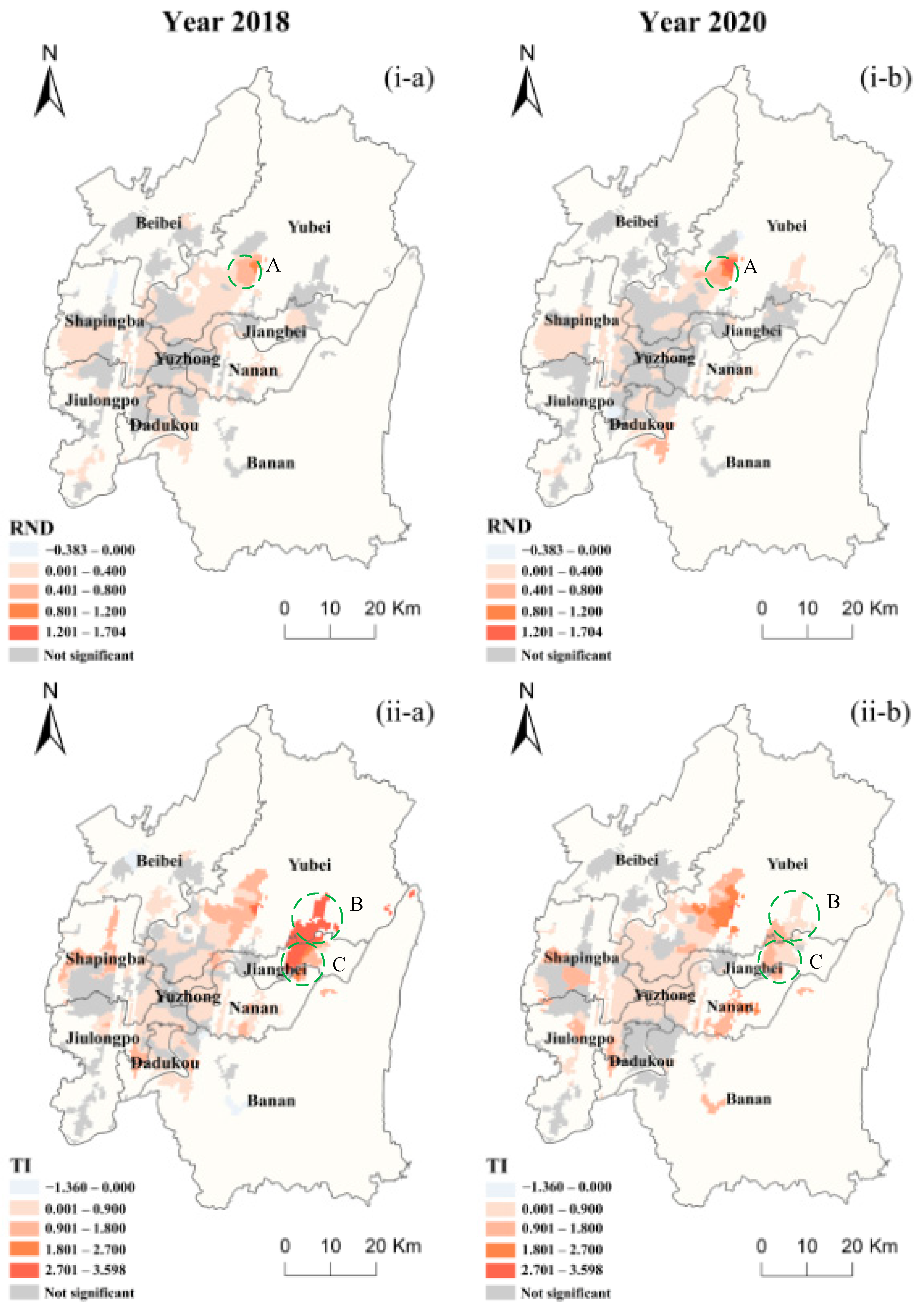
The spatial pattern of human activity feature contributions was explicitly demonstrated by the MGWR coefficients (Figure 4, Figure 5, Figure 6 and Figure 7). The traffic situation has a generally positive effect on the NTL intensity since the significant coefficients of RND and TI related to traffic are mainly positive in the two years of 2018 and 2020 (Figure 4). Specifically, the airport in Yubei (region A in Figure 4(i-a,i-b)) has the highest coefficients of RND and TI. Airport facilities and surrounding roads provide long-term and stable artificial light sources [7,64], and the light intensity provided by such facilities is also much higher than other urban areas. Moreover, different from road network, the contribution of transportation facilities varies greatly in different regions. The contribution of TI to NTL intensity has a decrement in the Longxing and Yufu areas (region B and C in Figure 4(ii-a,ii-b)), which are famous industrial centers in Chongqing and have a high density of expressway service facilities and gas stations. Originally, this kind of region promoted the NTL intensity according to its function. However, due to the COVID-19 pandemic in 2020, the human interactions in this region were restricted, which reduced the contribution of TI to NTL intensity [28,65,66]. It is worth noting that the contribution of RND to NTL intensity was not impacted by COVID-19 and the average contribution increased from 0.215 to 0.297 (Table 4). This is because the road network refers to the urban infrastructure construction, such as streetlights, which were lit during the COVID-19 period for citizens whether they were outdoors at night or not. Therefore, by comparing the changes in the traffic situation in the past two years, our model shows the possibility of exploring the industrial development state of some regions.
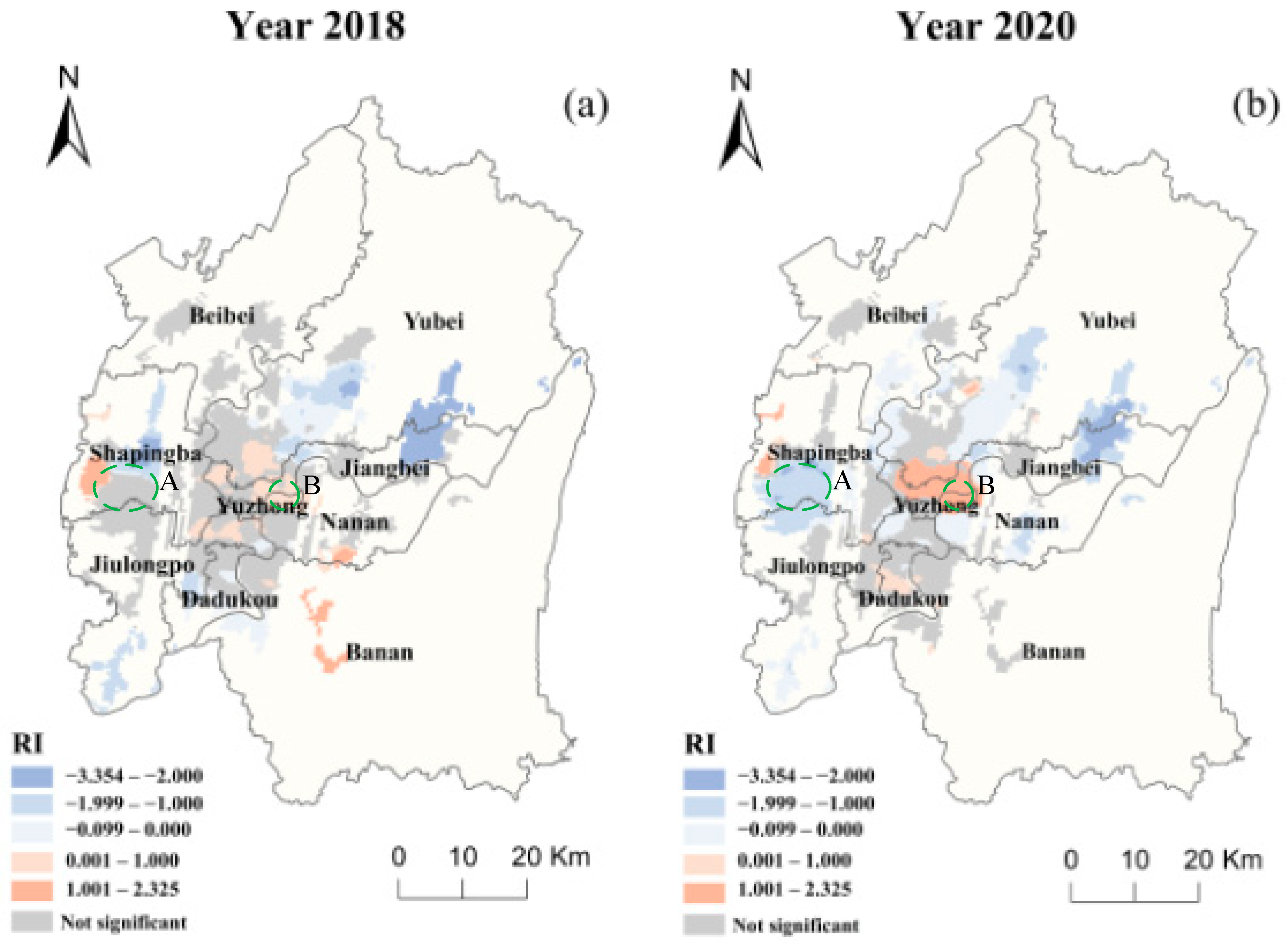
The residential area demoted the NTL intensity since the contribution of RI in most areas is negative. This is because the overpass time of the NPP satellite is about 1:30 AM, when most residents have turned off their indoor lights. From the temporal dynamics of the contribution of RI, there were more regions with negative contribution of RI in 2020 than in 2018, such as the western region of Shapingba (region A in Figure 5). This region, as a part of the Chongqing high-tech zone built in 2019, has many new residential areas. However, due to the relatively poor level of commercial, medical, educational, and other infrastructure in these regions, it has led to a slower inflow of population. These new residential areas cause a high vacancy issue in Chongqing [67], resulting in a negative impact on NTL intensity. It is noteworthy that the RI would have a positive effect to NTL intensity if the residential area was surrounded by commercial centers, such as the downtown area in Yuzhong (region B in Figure 5). In such an area, due to the high attraction of commercial centers, the human activity intensity from the nearby residential area can be much stronger than other residential areas and the interaction between the residential areas and shopping centers can be strong. Therefore, the light from the surrounding shopping malls can spill onto the nearby residential area. Our model shows the ability to evaluate the development level of residential areas in new urban areas.
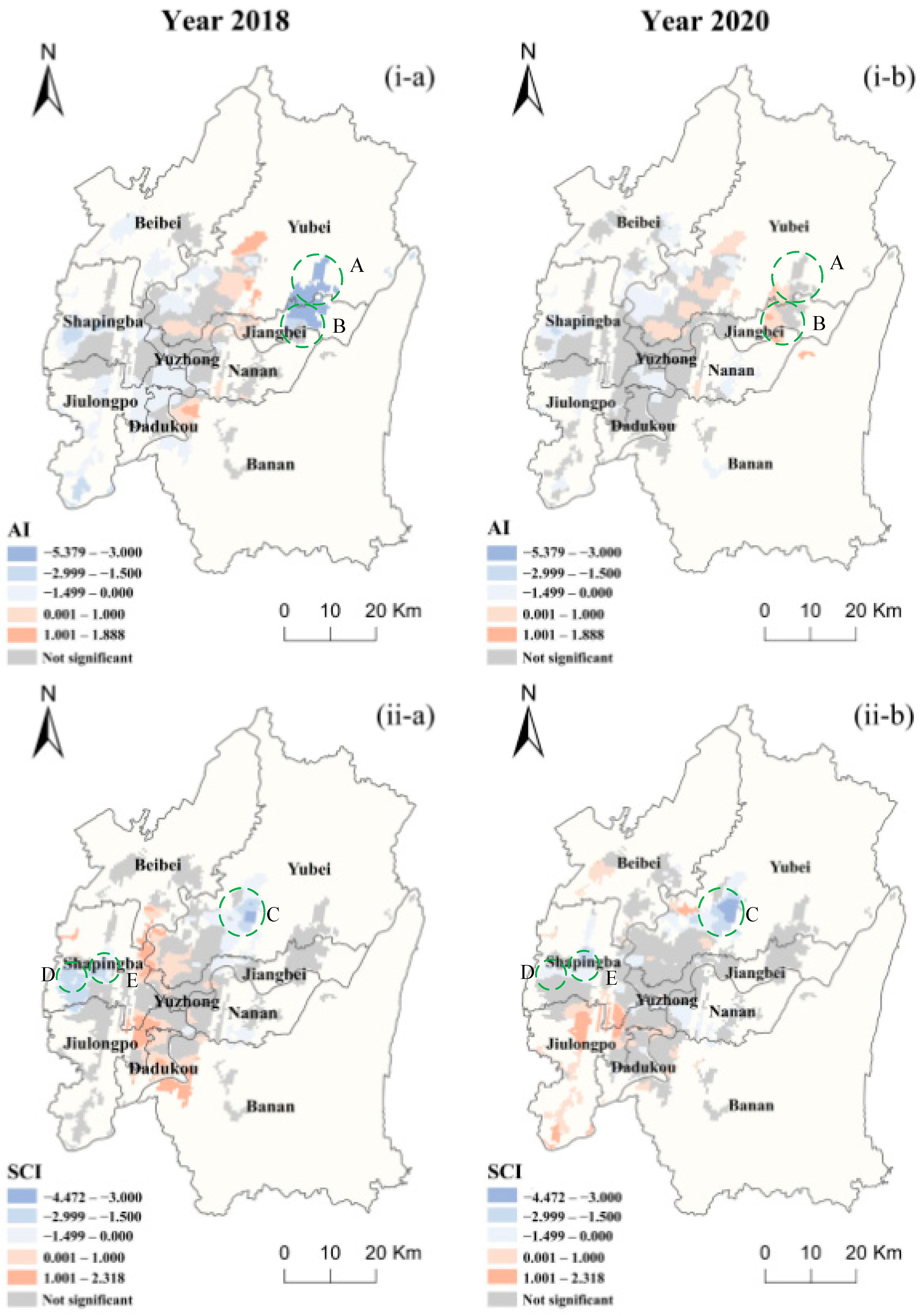
The administrative area showed a negative contribution to NTL intensity in the developed areas, but presented a positive contribution in the newly developing area (Figure 6(i-a,i-b)). Most government agencies mix with residential buildings in developed areas. These agencies cannot turn too many lights on at night to prevent the residents from light pollution, which leads to a negative contribution of AI to NTL intensity. In the newly developing area, the government agencies usually have their own buildings and are able to have better equipped lights [67]. Therefore, AI shows a positive effect in most of these areas, including parts of Jiangbei and Yubei (region A and B in Figure 6(i-a,i-b)). Most sport and cultural facilities (such as museums, libraries, sport stadiums, etc.) present a positive contribution to NTL intensity, especially when they are concentrated in the downtown area since they are always open to late at night. However, different from the facilities in the downtown area, when they are in the university campus (region D in Figure 6(ii-a,ii-b)), they close at night and turn off the lights to reduce energy consumption, which leads to a negative contribution of SCI to NTL intensity in this region. Meanwhile, if the sport and cultural facilities are discretely distributed, their contribution to NTL intensity is much worse. For example, the airport area (region C in Figure 6(ii-a,ii-b)) and Xiyong town (region E in Figure 6(ii-a,ii-b)) are the important transportation hub and industrial center of Chongqing, respectively. There are few sport and cultural facilities in these regions. These regions’ NTL intensity are mainly dominated by the traffic activity and production activity, rather than the sport or cultural activities.
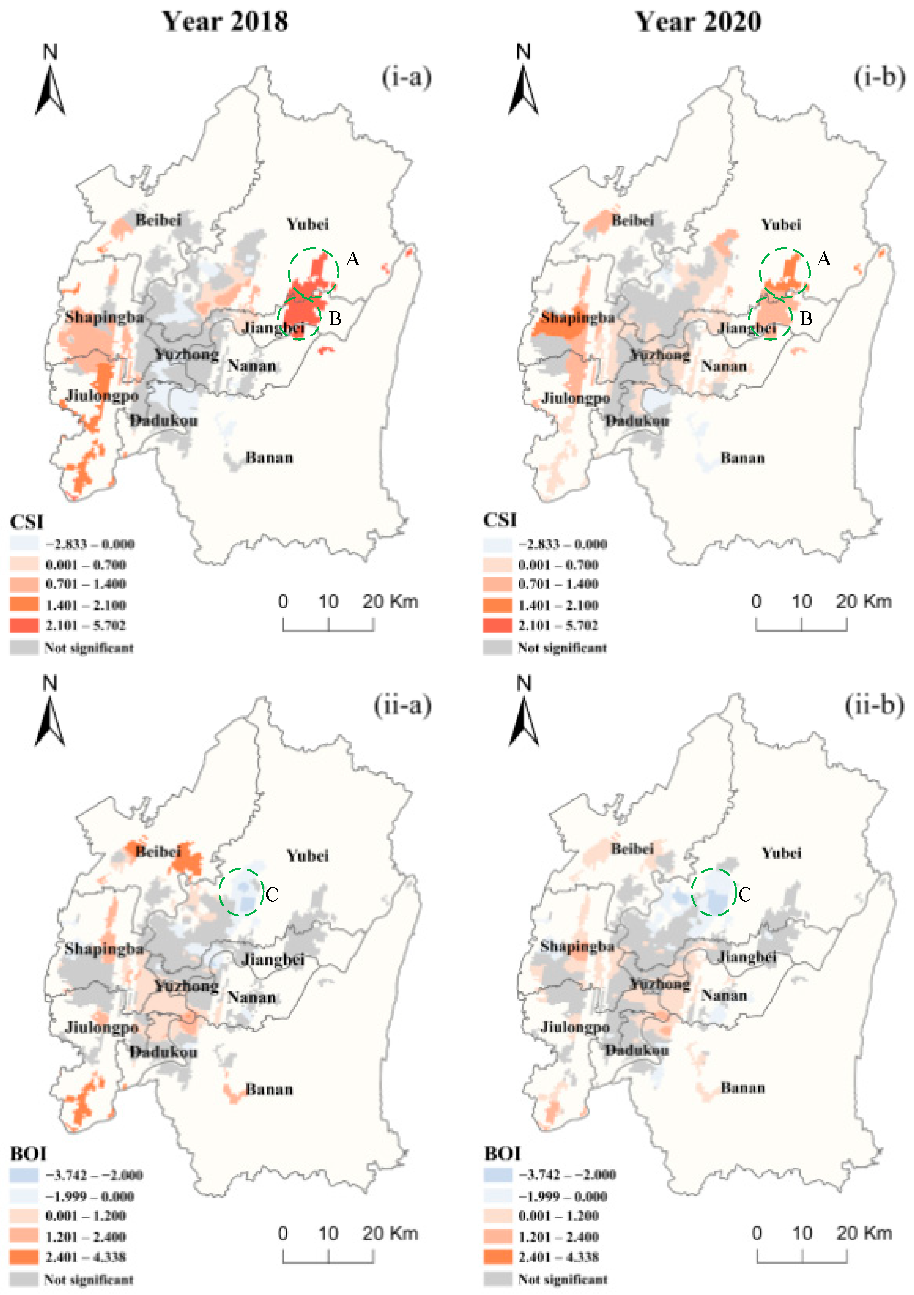
Our results show that commercial activities and business activities both have a strong contribution to NTL intensity, which is consistent with previous studies [33]. However, the average contribution of CSI to NTL intensity has a decrement of 32%, while the contribution of BOI has a much larger decrement of 81%. This might be caused by the different response of commercial and business activities when facing the COVID-19 pandemic. For instance, most commercial facilities (e.g., restaurants and supermarkets) were open in 2020, even though there were COVID-19 cases [68]. Therefore, commercial service facilities had a positive contribution to NTL intensity in most regions (Figure 7), except in some newly developing areas with the less permanent population (region A and B in Figure 7(i-a,i-b)) where lights were turned off to reduce cost. In contrast, most of the business offices have been closed during the COVID-19 pandemic, since the employees must work-from-home. Consequently, the contribution of BOI to NTL intensity has a larger reduction than the contribution of CSI. It is noteworthy that the business activities around the airport of Yubei (region C in Figure 7(ii-a,ii-b)) presented a negative contribution to NTL intensity in both years. This is similar to the negative contribution of SCI to NTL intensity mentioned before. The light from the transportation area is mainly derived from traffic facilities, instead of the seldom business activities.
The above analysis shows that the NTL data have greater potential to identify and monitor human activities and spatial patterns. By analyzing the change in RI’s contribution in the western of Shapingba (Figure 5), we found that many new residential buildings have been built here. However, the SCI’s (Figure 6(ii-a,ii-b)) contribution and BOI’s contribution (Figure 7(ii-a,ii-b)) have not increased significantly. As the prioritized region of the city, in the future policymakers can consider complementing relevant facilities (such as cultural facilities and companies) to attract the inflow of population and reduce the waste of land resources. Moreover, the MGWR model allows the variables to be assigned different bandwidths, which can avoid introducing too much noise and bias to improve the model fitting performance (Table 3). This finding has implications for expanding the application of NTL data. The MGWR model can be applied to downscale the NPP/VIIRS data to obtain long-term NTL data with higher spatial resolution.

6. Conclusions

Although previous studies have analyzed the relationship between human activities and light intensity from multiple perspectives, the influence of spatial heterogeneity on the results was rarely mentioned. In this study, MGWR was used for fitting, and the relationship between human activities and NPP/VIIRS NTL intensity in the study area was comprehensively analyzed. The results of the study indicate that the OLS and GWR regression models have difficulty explaining the spatial heterogeneity of the variables, and the performance of MGWR (adjusted R2 and AICc) was superior to OLS and GWR models. The road network density has the largest bandwidth, it represents relatively small spatial heterogeneity. Moreover, the NTL intensity was more sensitive to POI features, reflecting a larger spatial heterogeneity. From the comparison of regression coefficients between 2018 and 2020, the results showed that our model not only can explore the relationship between NTL intensity and human activity features, but also explains the spatial variation in the feature’s contribution. For example, we found that the contribution of road network density to NTL intensity changes relatively steady in space, because the streetlights can provide stable artificial light sources in urban areas. Furthermore, we found that the residential areas have an obviously heterogeneous distribution which is associated with the house vacancy. In addition, we noticed that most government agencies in developed areas have turned off many lights to protect residents from light pollution. Moreover, compared with the roads, the contribution of commercial service facilities and business offices in 2020 decreased to varying degrees, which was mainly caused by the restrictions on human activities due to COVID-19. By further analyzing the reasons for the change in the spatial pattern of feature contributions, which aims to facilitate the applications of NPP/VIIRS NTL data.
Our study successfully explores the relationship between NTL intensity and human activity features. However, there are some uncertainties and limitations that remain to be further improved. Firstly, although fitting results from the MGWR model were better than the GWR model, we noticed that the performance (adjusted R2 and AICc) improvement is not significant. The reasons may be due to study area and data quality issues (such as coarse spatial resolution of VIIRS data, and lack of a long time series of POI data). Since cities are complex systems and the urbanization process is a long-term process, future work is needed to reinforce the conclusions of this study by conducting long-term series studies in different cities. Second, some studies have shown that aerosol optical depth (AOD) are sensitive to the quality of NPP/VIIRS NTL images [69]. Limited by data availability, this paper only explores the influence of human activities to NTL intensity without considering the physical features. In further study, we should use data (e.g., AOD, LULC, and social media data) to reflect human and nature features for a comprehensive analysis. Finally, anisotropic characteristic [70,71] and seasonal changes (e.g., vegetation and snow cover) can also affect the NPP/VIIRS NTL intensity [7,72]. In order to better evaluate urban development, these factors need to be taken into account in future studies.

Author Contributions

Conceptualization Z.C.; methodology, J.W. and Z.C.; formal analysis, J.W.; writing—original draft preparation, J.W. and Z.C.; writing—review and editing, Z.C., Y.T. and B.Y.; funding acquisition, Z.C. and B.Y. All authors have read and agreed to the published version of the manuscript.

Funding

This research was funded by the National Natural Science Foundation of China (Grant No. 41871331 and 41801343), the Fundamental Research Funds for the Central Universities (Grant No. 2022ECNU-XWK-XK001), and the Innovation Program of Shanghai Municipal Education Commission (Grant No. 15ZZ026).

Data Availability Statement

The data presented in this study are available on request from the corresponding author.

Acknowledgments

We appreciate the critical and constructive comments and suggestions from the reviewers that helped improve the quality of this manuscript.

Conflicts of Interest

The authors declare no conflict of interest.

References

  1. Bennett, M.M.; Smith, L.C. Advances in using multitemporal night-time lights satellite imagery to detect, estimate, and monitor socioeconomic dynamics. Remote Sens. Environ. 2017, 192, 176–197. [Google Scholar] [CrossRef]
  2. Levin, N.; Kyba, C.C.M.; Zhang, Q.; Sánchez de Miguel, A.; Román, M.O.; Li, X.; Portnov, B.A.; Molthan, A.L.; Jechow, A.; Miller, S.D.; et al. Remote sensing of night lights: A review and an outlook for the future. Remote Sens. Environ. 2020, 237, 111443. [Google Scholar] [CrossRef]
  3. Elvidge, C.D.; Baugh, K.E.; Kihn, E.A.; Kroehl, H.W.; Davis, E.R.; Davis, C.W. Relation between satellite observed visible-near infrared emissions, population, economic activity and electric power consumption. Int. J. Remote Sens. 1997, 18, 1373–1379. [Google Scholar] [CrossRef]
  4. Imhoff, M.L.; Lawrence, W.T.; Elvidge, C.D.; Paul, T.; Levine, E.; Privalsky, M.V. Using nighttime DMSP/OLS images of city lights to estimate the impact of urban land use on soil resources in the United States. Remote Sens. Environ. 1997, 59, 105–117. [Google Scholar] [CrossRef]
  5. Small, C.; Pozzi, F.; Elvidge, C.D. Spatial analysis of global urban extent from DMSP-OLS night lights. Remote Sens. Environ. 2005, 96, 277–291. [Google Scholar] [CrossRef]
  6. Ghosh, T.; Sutton, P.; Powell, R.; Anderson, S.; Elvidge, C.D. Estimation of Mexico’s Informal Economy Using DMSP Nighttime Lights Data. In Proceedings of the 2009 Joint Urban Remote Sensing Event, Shanghai, China, 20–22 May 2009; Volume 1–3, p. 1675. [Google Scholar]
  7. Levin, N.; Zhang, Q. A global analysis of factors controlling VIIRS nighttime light levels from densely populated areas. Remote Sens. Environ. 2017, 190, 366–382. [Google Scholar] [CrossRef] [Green Version]
  8. Stokes, E.C.; Seto, K.C. Characterizing urban infrastructural transitions for the Sustainable Development Goals using multi-temporal land, population, and nighttime light data. Remote Sens. Environ. 2019, 234, 111430. [Google Scholar] [CrossRef]
  9. Keola, S.; Andersson, M.; Hall, O. Monitoring Economic Development from Space: Using Nighttime Light and Land Cover Data to Measure Economic Growth. World Dev. 2015, 66, 322–334. [Google Scholar] [CrossRef]
  10. Wang, X.; Sutton, P.C.; Qi, B. Global Mapping of GDP at 1 km2 Using VIIRS Nighttime Satellite Imagery. ISPRS Int. J. Geo-Inf. 2019, 8, 580. [Google Scholar] [CrossRef] [Green Version]
  11. Zhou, Y.; Smith, S.J.; Elvidge, C.D.; Zhao, K.; Thomson, A.; Imhoff, M. A cluster-based method to map urban area from DMSP/OLS nightlights. Remote Sens. Environ. 2014, 147, 173–185. [Google Scholar] [CrossRef]
  12. Yu, B.; Tang, M.; Wu, Q.; Yang, C.; Deng, S.; Shi, K.; Peng, C.; Wu, J.; Chen, Z. Urban Built-Up Area Extraction From Log- Transformed NPP-VIIRS Nighttime Light Composite Data. IEEE Geosci. Remote Sens. Lett. 2018, 15, 1279–1283. [Google Scholar] [CrossRef]
  13. Sutton, P. Modeling population density with night-time satellite imagery and GIS. Comput. Environ. Urban Syst. 1997, 21, 227–244. [Google Scholar] [CrossRef]
  14. Zhuo, L.; Ichinose, T.; Zheng, J.; Chen, J.; Shi, P.J.; Li, X. Modelling the population density of China at the pixel level based on DMSP/OLS non-radiance-calibrated night-time light images. Int. J. Remote Sens. 2009, 30, 1003–1018. [Google Scholar] [CrossRef]
  15. Sun, W.; Zhang, X.; Wang, N.; Cen, Y. Estimating Population Density Using DMSP-OLS Night-Time Imagery and Land Cover Data. IEEE J. Sel. Top. Appl. Earth Obs. Remote Sens. 2017, 10, 2674–2684. [Google Scholar] [CrossRef]
  16. Yu, B.; Lian, T.; Huang, Y.; Yao, S.; Ye, X.; Chen, Z.; Yang, C.; Wu, J. Integration of nighttime light remote sensing images and taxi GPS tracking data for population surface enhancement. Int. J. Geogr. Inf. Sci. 2018, 33, 687–706. [Google Scholar] [CrossRef]
  17. Chen, Z.; Yu, B.; Hu, Y.; Huang, C.; Shi, K.; Wu, J. Estimating House Vacancy Rate in Metropolitan Areas Using NPP-VIIRS Nighttime Light Composite Data. IEEE J. Sel. Top. Appl. Earth Obs. Remote Sens. 2015, 8, 2188–2197. [Google Scholar] [CrossRef]
  18. Jean, N.; Burke, M.; Xie, M.; Davis, W.M.; Lobell, D.B.; Ermon, S. Combining satellite imagery and machine learning to predict poverty. Science 2016, 353, 790–794. [Google Scholar] [CrossRef] [Green Version]
  19. Shi, K.; Chang, Z.; Chen, Z.; Wu, J.; Yu, B. Identifying and evaluating poverty using multisource remote sensing and point of interest (POI) data: A case study of Chongqing, China. J. Clean. Prod. 2020, 255, 120245. [Google Scholar] [CrossRef]
  20. Xie, Y.; Weng, Q.; Fu, P. Temporal variations of artificial nighttime lights and their implications for urbanization in the conterminous United States, 2013–2017. Remote Sens. Environ. 2019, 225, 160–174. [Google Scholar] [CrossRef]
  21. Letu, H.; Hara, M.; Yagi, H.; Naoki, K.; Tana, G.; Nishio, F.; Shuhei, O. Estimating energy consumption from night-time DMPS/OLS imagery after correcting for saturation effects. Int. J. Remote Sens. 2010, 31, 4443–4458. [Google Scholar] [CrossRef]
  22. Shi, K.; Yu, B.; Huang, C.; Wu, J.; Sun, X. Exploring spatiotemporal patterns of electric power consumption in countries along the Belt and Road. Energy 2018, 150, 847–859. [Google Scholar] [CrossRef]
  23. Wang, J.; Lu, F. Modeling the electricity consumption by combining land use types and landscape patterns with nighttime light imagery. Energy 2021, 234, 121305. [Google Scholar] [CrossRef]
  24. Shi, K.; Chen, Y.; Yu, B.; Xu, T.; Chen, Z.; Liu, R.; Li, L.; Wu, J. Modeling spatiotemporal CO2 (carbon dioxide) emission dynamics in China from DMSP-OLS nighttime stable light data using panel data analysis. Appl. Energy 2016, 168, 523–533. [Google Scholar] [CrossRef]
  25. Kuechly, H.U.; Kyba, C.C.M.; Ruhtz, T.; Lindemann, C.; Wolter, C.; Fischer, J.; Hölker, F. Aerial survey and spatial analysis of sources of light pollution in Berlin, Germany. Remote Sens. Environ. 2012, 126, 39–50. [Google Scholar] [CrossRef]
  26. Bennie, J.; Davies, T.W.; Duffy, J.P.; Inger, R.; Gaston, K.J. Contrasting trends in light pollution across Europe based on satellite observed night time lights. Sci. Rep. 2014, 4, 3789. [Google Scholar] [CrossRef] [Green Version]
  27. Kloog, I.; Haim, A.; Stevens, R.G.; Portnov, B.A. Global co-distribution of light at night (LAN) and cancers of prostate, colon, and lung in men. Chronobiol. Int. 2009, 26, 108–125. [Google Scholar] [CrossRef]
  28. Straka, W.; Kondragunta, S.; Wei, Z.; Zhang, H.; Miller, S.D.; Watts, A. Examining the Economic and Environmental Impacts of COVID-19 Using Earth Observation Data. Remote Sens. 2020, 13, 5. [Google Scholar] [CrossRef]
  29. Li, X.-Y.; Li, X.; Fan, Z.; Mi, L.; Kandakji, T.; Song, Z.; Li, D.; Song, X.-P. Civil war hinders crop production and threatens food security in Syria. Nat. Food 2022, 3, 38–46. [Google Scholar] [CrossRef]
  30. Elvidge, C.D.; Baugh, K.E.; Zhizhin, M.; Hsu, F.-C. Why VIIRS data are superior to DMSP for mapping nighttime lights. Proc. Asia-Pac. Adv. Netw. 2013, 35, 62. [Google Scholar] [CrossRef] [Green Version]
  31. Li, X.; Ge, L.; Chen, X. Quantifying Contribution of Land Use Types to Nighttime Light Using an Unmixing Model. IEEE Geosci. Remote Sens. Lett. 2014, 11, 1667–1671. [Google Scholar] [CrossRef]
  32. Ma, T. An Estimate of the Pixel-Level Connection between Visible Infrared Imaging Radiometer Suite Day/Night Band (VIIRS DNB) Nighttime Lights and Land Features across China. Remote Sens. 2018, 10, 723. [Google Scholar] [CrossRef] [Green Version]
  33. Chen, Y.; Liu, X.; Li, X. Analyzing Parcel-Level Relationships between Urban Land Expansion and Activity Changes by Integrating Landsat and Nighttime Light Data. Remote Sens. 2017, 9, 164. [Google Scholar] [CrossRef] [Green Version]
  34. Wang, C.; Chen, Z.; Yang, C.; Li, Q.; Wu, Q.; Wu, J.; Zhang, G.; Yu, B. Analyzing parcel-level relationships between Luojia 1-01 nighttime light intensity and artificial surface features across Shanghai, China: A comparison with NPP-VIIRS data. Int. J. Appl. Earth Obs. Geoinf. 2020, 85, 101989. [Google Scholar] [CrossRef]
  35. Song, J.; Tong, X.; Wang, L.; Zhao, C.; Prishchepov, A.V. Monitoring finer-scale population density in urban functional zones: A remote sensing data fusion approach. Landsc. Urban Plan. 2019, 190, 103580. [Google Scholar] [CrossRef]
  36. Brunsdon, C.; Fotheringham, A.S.; Charlton, M.E. Geographically weighted regression: A method for exploring spatial nonstationarity. Geogr. Anal. 1996, 28, 281–298. [Google Scholar] [CrossRef]
  37. Brunsdon, C.; Fotheringham, A.S.; Charlton, M. Some notes on parametric significance tests for geographically weighted regression. J. Reg. Sci. 1999, 39, 497–524. [Google Scholar] [CrossRef]
  38. Ye, Y.; Huang, L.; Zheng, Q.; Liang, C.; Dong, B.; Deng, J.; Han, X. A feasible framework to downscale NPP-VIIRS nighttime light imagery using multi-source spatial variables and geographically weighted regression. Int. J. Appl. Earth Obs. Geoinf. 2021, 104, 102513. [Google Scholar] [CrossRef]
  39. Fotheringham, A.S.; Yang, W.; Kang, W. Multiscale Geographically Weighted Regression (MGWR). Ann. Am. Assoc. Geogr. 2017, 107, 1247–1265. [Google Scholar] [CrossRef]
  40. Liu, P.; Wu, C.; Chen, M.; Ye, X.; Peng, Y.; Li, S. A Spatiotemporal Analysis of the Effects of Urbanization’s Socio-Economic Factors on Landscape Patterns Considering Operational Scales. Sustainability 2020, 12, 2543. [Google Scholar] [CrossRef] [Green Version]
  41. Mansour, S.; Al Kindi, A.; Al-Said, A.; Al-Said, A.; Atkinson, P. Sociodemographic determinants of COVID-19 incidence rates in Oman: Geospatial modelling using multiscale geographically weighted regression (MGWR). Sustain. Cities Soc. 2021, 65, 102627. [Google Scholar] [CrossRef]
  42. Liu, H.; Huang, B.; Gao, S.; Wang, J.; Yang, C.; Li, R. Impacts of the evolving urban development on intra-urban surface thermal environment: Evidence from 323 Chinese cities. Sci. Total Environ. 2021, 771, 144810. [Google Scholar] [CrossRef] [PubMed]
  43. Gu, H.; Yu, H.; Sachdeva, M.; Liu, Y. Analyzing the distribution of researchers in China: An approach using multiscale geographically weighted regression. Growth Chang. 2020, 52, 443–459. [Google Scholar] [CrossRef]
  44. Niu, L.; Zhang, Z.; Peng, Z.; Liang, Y.; Liu, M.; Jiang, Y.; Wei, J.; Tang, R. Identifying Surface Urban Heat Island Drivers and Their Spatial Heterogeneity in China’s 281 Cities: An Empirical Study Based on Multiscale Geographically Weighted Regression. Remote Sens. 2021, 13, 4428. [Google Scholar] [CrossRef]
  45. Oshan, T.M.; Smith, J.P.; Fotheringham, A.S. Targeting the spatial context of obesity determinants via multiscale geographically weighted regression. Int. J. Health Geogr. 2020, 19, 11. [Google Scholar] [CrossRef] [PubMed]
  46. Mollalo, A.; Vahedi, B.; Rivera, K.M. GIS-based spatial modeling of COVID-19 incidence rate in the continental United States. Sci. Total Environ. 2020, 728, 138884. [Google Scholar] [CrossRef]
  47. Cai, J.; Huang, B.; Song, Y. Using multi-source geospatial big data to identify the structure of polycentric cities. Remote Sens. Environ. 2017, 202, 210–221. [Google Scholar] [CrossRef]
  48. Yan, J.; Yang, Z.; Li, Z.; Li, X.; Xin, L.; Sun, L. Drivers of cropland abandonment in mountainous areas: A household decision model on farming scale in Southwest China. Land Use Policy 2016, 57, 459–469. [Google Scholar] [CrossRef] [Green Version]
  49. Elvidge, C.D.; Zhizhin, M.; Ghosh, T.; Hsu, F.-C.; Taneja, J. Annual Time Series of Global VIIRS Nighttime Lights Derived from Monthly Averages: 2012 to 2019. Remote Sens. 2021, 13, 922. [Google Scholar] [CrossRef]
  50. Gong, P.; Chen, B.; Li, X.; Liu, H.; Wang, J.; Bai, Y.; Chen, J.; Chen, X.; Fang, L.; Feng, S.; et al. Mapping essential urban land use categories in China (EULUC-China): Preliminary results for 2018. Sci. Bull. 2020, 65, 182–187. [Google Scholar] [CrossRef] [Green Version]
  51. Dobler, G.; Ghandehari, M.; Koonin, S.E.; Nazari, R.; Patrinos, A.; Sharma, M.S.; Tafvizi, A.; Vo, H.T.; Wurtele, J.S. Dynamics of the urban lightscape. Inf. Syst. 2015, 54, 115–126. [Google Scholar] [CrossRef]
  52. Cheng, B.; Chen, Z.; Yu, B.; Li, Q.; Wang, C.; Li, B.; Wu, B.; Li, Y.; Wu, J. Automated Extraction of Street Lights From JL1-3B Nighttime Light Data and Assessment of Their Solar Energy Potential. IEEE J. Sel. Top. Appl. Earth Obs. Remote Sens. 2020, 13, 675–684. [Google Scholar] [CrossRef]
  53. Zhou, Y.; Li, X.; Asrar, G.R.; Smith, S.J.; Imhoff, M. A global record of annual urban dynamics (1992–2013) from nighttime lights. Remote Sens. Environ. 2018, 219, 206–220. [Google Scholar] [CrossRef]
  54. Wang, L.; Li, C.; Ying, Q.; Cheng, X.; Wang, X.; Li, X.; Hu, L.; Liang, L.; Yu, L.; Huang, H.; et al. China’s urban expansion from 1990 to 2010 determined with satellite remote sensing. Chin. Sci. Bull. 2012, 57, 2802–2812. [Google Scholar] [CrossRef] [Green Version]
  55. Li, X.; Gong, P.; Zhou, Y.; Wang, J.; Bai, Y.; Chen, B.; Hu, T.; Xiao, Y.; Xu, B.; Yang, J.; et al. Mapping global urban boundaries from the global artificial impervious area (GAIA) data. Environ. Res. Lett. 2020, 15, 094044. [Google Scholar] [CrossRef]
  56. Oshan, T.; Li, Z.; Kang, W.; Wolf, L.; Fotheringham, A. mgwr: A Python Implementation of Multiscale Geographically Weighted Regression for Investigating Process Spatial Heterogeneity and Scale. ISPRS Int. J. Geo-Inf. 2019, 8, 269. [Google Scholar] [CrossRef] [Green Version]
  57. Shi, X. Selection of bandwidth type and adjustment side in kernel density estimation over inhomogeneous backgrounds. Int. J. Geogr. Inf. Sci. 2010, 24, 643–660. [Google Scholar] [CrossRef]
  58. Fotheringham, A.S.; Brunsdon, C. Local forms of spatial analysis. Geogr. Anal. 1999, 31, 340–358. [Google Scholar] [CrossRef]
  59. Fotheringham, A.S.; Oshan, T.M. Geographically weighted regression and multicollinearity: Dispelling the myth. J. Geogr. Syst. 2016, 18, 303–329. [Google Scholar] [CrossRef]
  60. Wolf, L.J.; Oshan, T.M.; Fotheringham, A.S. Single and Multiscale Models of Process Spatial Heterogeneity. Geogr. Anal. 2018, 50, 223–246. [Google Scholar] [CrossRef] [Green Version]
  61. Yu, H.; Fotheringham, A.S.; Li, Z.; Oshan, T.; Wolf, L.J. On the measurement of bias in geographically weighted regression models. Spat. Stat. 2020, 38, 100453. [Google Scholar] [CrossRef]
  62. Chen, Y.; Zhu, M.; Zhou, Q.; Qiao, Y. Research on Spatiotemporal Differentiation and Influence Mechanism of Urban Resilience in China Based on MGWR Model. Int. J. Environ. Res. Public Health 2021, 18, 1056. [Google Scholar] [CrossRef] [PubMed]
  63. Xue, C.; Chen, X.; Xue, L.; Zhang, H.; Chen, J.; Li, D. Modeling the spatially heterogeneous relationships between tradeoffs and synergies among ecosystem services and potential drivers considering geographic scale in Bairin Left Banner, China. Sci. Total Environ. 2022, 855, 158834. [Google Scholar] [CrossRef] [PubMed]
  64. Wu, J.; Zhang, Z.; Yang, X.; Li, X. Analyzing Pixel-Level Relationships between Luojia 1-01 Nighttime Light and Urban Surface Features by Separating the Pixel Blooming Effect. Remote Sens. 2021, 13, 4838. [Google Scholar] [CrossRef]
  65. Elvidge, C.; Ghosh, T.; Hsu, F.-C.; Zhizhin, M.; Bazilian, M. The Dimming of Lights in China during the COVID-19 Pandemic. Remote Sens. 2020, 12, 2851. [Google Scholar] [CrossRef]
  66. Saadat, S.; Rawtani, D.; Hussain, C.M. Environmental perspective of COVID-19. Sci. Total Environ. 2020, 728, 138870. [Google Scholar] [CrossRef]
  67. Liu, Y.; Fan, P.; Yue, W.; Song, Y. Impacts of land finance on urban sprawl in China: The case of Chongqing. Land Use Policy 2018, 72, 420–432. [Google Scholar] [CrossRef]
  68. Liu, Q.; Sha, D.; Liu, W.; Houser, P.; Zhang, L.; Hou, R.; Lan, H.; Flynn, C.; Lu, M.; Hu, T.; et al. Spatiotemporal Patterns of COVID-19 Impact on Human Activities and Environment in Mainland China Using Nighttime Light and Air Quality Data. Remote Sens. 2020, 12, 1576. [Google Scholar] [CrossRef]
  69. Wang, X.; Mu, X.; Yan, G. Quantitative Analysis of Aerosol Influence on Suomi-NPP VIIRS Nighttime Light in China. IEEE J. Sel. Top. Appl. Earth Obs. Remote Sens. 2020, 13, 3557–3568. [Google Scholar] [CrossRef]
  70. Li, X.; Ma, R.; Zhang, Q.; Li, D.; Liu, S.; He, T.; Zhao, L. Anisotropic characteristic of artificial light at night—Systematic investigation with VIIRS DNB multi-temporal observations. Remote Sens. Environ. 2019, 233, 111357. [Google Scholar] [CrossRef]
  71. Li, X.; Shang, X.; Zhang, Q.; Li, D.; Chen, F.; Jia, M.; Wang, Y. Using radiant intensity to characterize the anisotropy of satellite-derived city light at night. Remote Sens. Environ. 2022, 271, 112920. [Google Scholar] [CrossRef]
  72. Chen, Z.; Yu, B.; Ta, N.; Shi, K.; Yang, C.; Wang, C.; Zhao, X.; Deng, S.; Wu, J. Delineating Seasonal Relationships Between Suomi NPP-VIIRS Nighttime Light and Human Activity Across Shanghai, China. IEEE J. Sel. Top. Appl. Earth Obs. Remote Sens. 2019, 12, 4275–4283. [Google Scholar] [CrossRef]
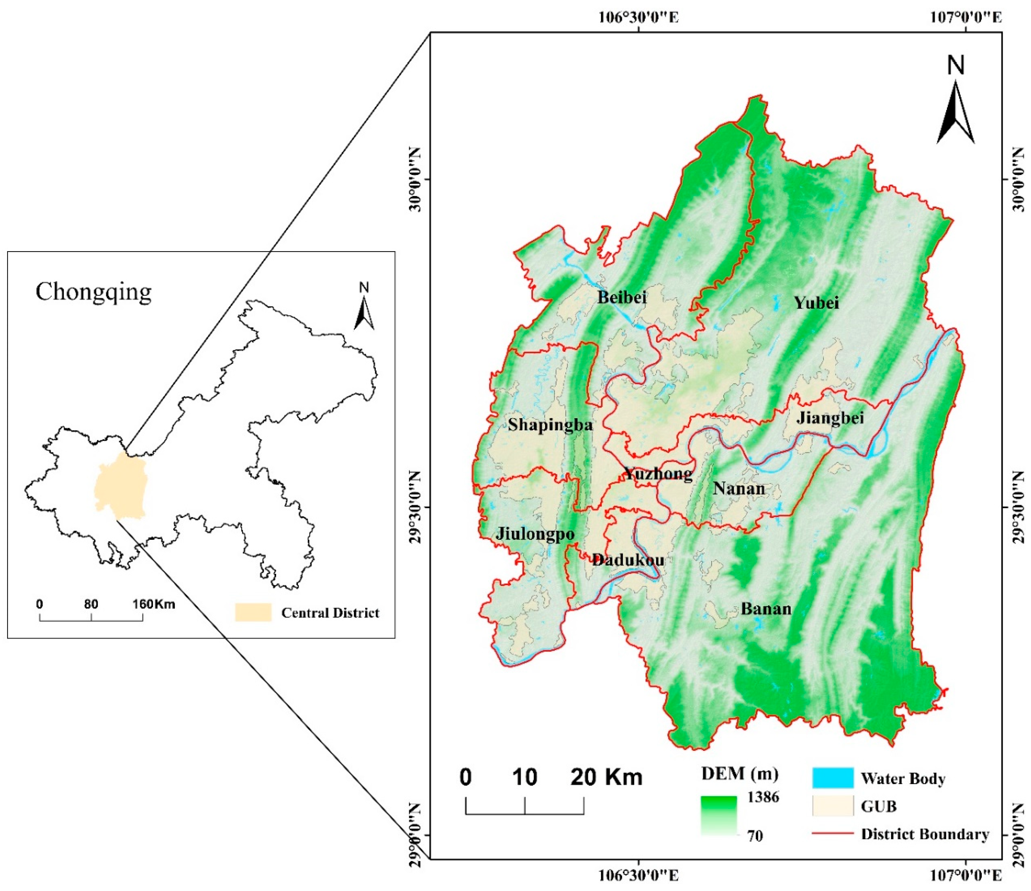
Figure 1. Location of the study area (DEM: digital elevation model; GUBs: global urban boundaries).
Remotesensing 14 05695 g001
Figure 2. Spatial distribution of data used in this study in 2018: (a) NPP/VIIRS NTL image; (b) residential POI data; (c) businesses office POI data; (d) commercial service POI data; (e) transportation POI data; (f) administrative POI data; (g) sports and cultural POI data and (h) road network composed with all levels of roads.
Remotesensing 14 05695 g002
Figure 3. The overall framework of the study.
Remotesensing 14 05695 g003
Figure 4. Spatial distributions of the coefficients of (i) road network density and (ii) transportation index in (a) 2018 and (b) 2020 (RND: road network density; TI: transportation index; Region A is the Airport; Region B is the Longxing town; Region C is the Yufu town).
Remotesensing 14 05695 g004
Figure 5. Spatial distributions of the coefficients of residential index in (a) 2018 and (b) 2020 (RI: residential index; Region A is the residential agglomeration in Shapingba; Region B is the residential agglomeration in Yuzhon).
Remotesensing 14 05695 g005
Figure 6. Spatial distributions of the coefficients of (i) administrative index and (ii) sport and cultural index in (a) 2018 and (b) 2020 (AI: administrative index; SCI: sport and cultural index. Region A is the Longxing town; Region B is the Yufu town; Region C is the Airport; Region D is the University town; Region E is the Xiyong town).
Remotesensing 14 05695 g006
Figure 7. Spatial distributions of the coefficients of (i) commercial services index and () business office index in (a) 2018 and (b) 2020 (CSI: commercial service index; BOI: business office index. Region A is the Longxing town; Region B is the Yufu town; Region C is the Airport).
Remotesensing 14 05695 g007
Table 1. The description of POI data categories.
Reclassified POI CategoriesOriginal POI CategoriesCount (2018)Count (2020)
ResidentialResidential12,98713,578
Business officeBank, Company, Factory, Finance and Insurance Service Institution, etc.45,15246,008
Commercial serviceRestaurant, Theatre and Cinema, Recreation Center, Supermarket, Shopping Related Places, etc.49,61848,430
TransportationAirport, Railway Station, Subway Station, Bus Station, Expressway Service Area, Filling Station, etc.13,93414,524
AdministrativeGovernmental Organization, Public service agencies, etc.19,47420,545
Sports and culturalMuseum, Exhibition Center, Library, Cultural Palace, Sports Stadium, etc.11,27212,369
Table 2. Descriptive statistics for variables in this study.
Variable *MeanStandard DeviationMinimumMaximum
20182020201820202018202020182020
RND7.857.925.675.650039.2141.76
TI7.507.647.968.450094.56105.37
RI10.111.3214.8716.060091.7792.05
AI12.4613.7620.8211.5700184.7180.27
SCI8.888.5918.3510.4800181.85170.70
CSI39.7942.3174.8898.5900739.39933.63
BOI27.1529.2550.0439.3500475.10380.27
* RND: road network density; TI: transportation index; RI: residential index; AI: administrative index; SCI: sport and cultural index; CSI: commercial service index; BOI: business office index.
Table 3. Comparing the OLS, GWR, and MGWR model fits.
ModelAdj.R2 *AICc *RSS *
201820202018202020182020
OLS0.250.2911,046.7510,811.923249.253074.89
GWR0.850.865366.544840.46503.29460.76
MGWR0.860.874844.634623.27415.30392.28
* Adj.R2: adjusted coefficient of determination; AICc: corrected Akaike Information Criterion; RSS: residual sum of squares.
Table 4. The spatial bandwidths of the MGWR models.
VariableGWR ModelMGWR Model
2018202020182020
Road network density (RND)5865128142
Transportation index (TI)4343
Residential index (RI)4646
Administrative index (AI)4343
Sport and cultural index (SCI)4343
Commercial service index (CSI)4343
Business office index (BOI)4346
Table 5. The MGWR coefficients of 7 variables in 2018 and 2020.
Variable *Coefficients in 2018 (p < 0.05)Coefficients in 2020 (p < 0.05)
MinimumMaximumMeanMinimumMaximumMean
RND−0.2631.2810.215−0.3831.7040.297
TI−1.3603.5980.885−0.6962.9550.826
RI−3.3542.325−0.818−2.2891.980−0.674
AI−5.3791.931−0.918−1.9031.342−0.255
SCI−4.3542.158−0.255−4.4722.318−0.246
CSI−2.8335.7020.956−0.3121.5330.648
BOI−3.7424.3380.898−3.6111.9640.165
* RND: road network density; TI: transportation index; RI: residential index; AI: administrative index; SCI: sport and cultural index; CSI: commercial service index; BOI: business office index.
Publisher’s Note: MDPI stays neutral with regard to jurisdictional claims in published maps and institutional affiliations.